Journal of Ecology ( IF 5.3 ) Pub Date : 2022-08-03 , DOI: 10.1111/1365-2745.13980 Bin J. W. Chen 1 , Shuqing N. Teng 2 , Guang Zheng 3 , Lijuan Cui 4 , Shao‐Peng Li 5 , Arie Staal 6 , Jan U. H. Eitel 7, 8 , Thomas W. Crowther 9 , Miguel Berdugo 9 , Mo Lidong 9 , Haozhi Ma 9 , Lalasia Bialic‐Murphy 9 , Constantin M. Zohner 9 , Daniel Maynard 9 , Colin Averill 9 , Jian Zhang 10 , Qiang He 11 , Jochem B. Evers 12 , Niels P. R. Anten 12 , Hezi Yizhaq 13 , Ilan Stavi 14 , Eli Argaman 15 , Uri Basson 16 , Zhiwei Xu 17 , Ming‐Juan Zhang 18 , Kechang Niu 2 , Quan‐Xing Liu 10 , Chi Xu 2
|
1 INTRODUCTION
The use of remote sensing technologies to capture broad-scale ecological patterns is rapidly expanding. In plant ecology, the enhanced ability of remote sensing to collect biophysical and physiological data opens a wide range of opportunities to systematically characterise the development and performance of individual plants, the composition and structure of plant communities, and the functioning and dynamics of ecosystems in a fast, non-destructive way, at multiple spatiotemporal scales (Gamon et al., 2016; Magney et al., 2019; Zellweger et al., 2019). Despite the continuous developments, remote-sensing applications lack significant capacities, especially regarding the inference of key ecological processes. For example, it is notoriously challenging to remotely sense how plants interact with one another, which is a central question in plant ecology. Plant–plant interactions often act as key drivers of community assembly and functioning (Bilas et al., 2021) and determine evolutionary processes (Thorpe et al., 2011). They also play a central role in dictating primary productivity (Postma et al., 2021) and mediating climate change impacts on ecosystems (van Loon et al., 2014).
Inferring the direction and magnitude of plant–plant interactions has strongly relied on manipulative experiments that are labour-intensive and time-consuming and are therefore often restricted to small spatiotemporal scales (Schöb et al., 2012). Also, traditional approaches often interfere with the studied system, hampering result replication (Catchpole & Wheeler, 1992; Jimenez-Berni et al., 2018). These drawbacks typically fall into the domain where remote sensing technologies have clear advantages. However, the link between plant–plant interactions and remote sensing indicators remains elusive.
- Competition and facilitation—which are the key interactions in shaping plant communities (Holmgren et al., 1997).
-
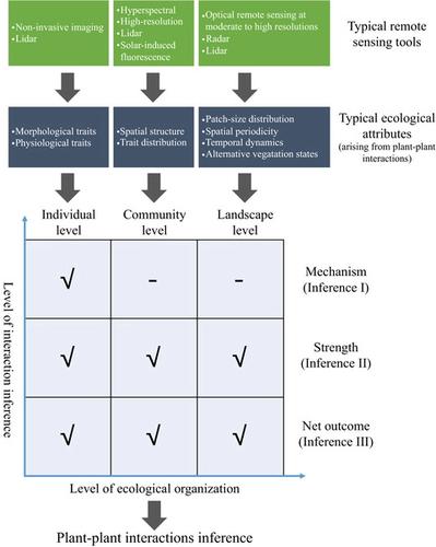
Three types of interaction inference:
- mechanisms of pairwise plant–plant interactions (Inference I);
- relative strengths of particular plant–plant interactions (Inference II);
- emerging net outcomes of co-occurring plant–plant interactions (Inference III).
-
Three levels of ecological organization:
- individual level (Section 2), at which interactions have typically been inferred by changes of morphological, physiological and functional traits of interacting plant individuals/species in the field or in experimental settings;
- community level (Section 3), at which interactions have typically been inferred by scrutinizing spatial and functional structures (e.g., over- or under-dispersion) of plant communities. While the term ‘community’ may be used for a wide range of spatial scales (Vellend, 2016), here the community level is restricted to a field plot scale, typically 10–100 m2.
- landscape level (Section 4), at which landscape patterns and states, in combination with theoretical models, can indicate interactions from snapshots or time series of remote sensing data.

At each level, we summarize the key plant–plant interaction outcomes captured by remote sensing data (Table 1) and review the relevant theoretical bases and approaches of how plant–plant interactions can be inferred by remotely measuring these outcomes. This non-exhaustive review focuses on key ideas, transformative approaches, major challenges and future outlooks toward building rigorous links between remote sensing and ‘cryptic’ biotic interactions.
| Level | Attributes measured | Typical remote sensing tools | Inference | |
|---|---|---|---|---|
| Individual | Whole plant | Volume, height, biomass | Non-invasive imaging, lidar | II & III |
| Leaf | Size (e.g., length, wise, area, volume) | Non-invasive imaging, lidar | II & III | |
| Posture (e.g., zenith, azimuth and dihedral angles) | Non-invasive imaging, lidar | I, II & III | ||
| Chemistry (e.g., chlorophyll, water, nutrients, structural and defence components) | Hyperspectral, multispectral, lidar | I & II | ||
| Temperature | Thermal imaging | II | ||
| Branch | Size (e.g., length, diameter, volume) | Non-invasive imaging, lidar | II & III | |
| Posture (e.g., zenith, azimuth, and dihedral angles) | I & II | |||
| Spatial occupation within crown | II & III | |||
| Crown | Size (length, width, depth, volume, projected leaf area) | Non-invasive imaging, lidar | II & III | |
| Openness, foliar density, branch density | II & III | |||
| Foliar physical profile (area, volume) | I & II | |||
| Foliar chemical profile (e.g., chlorophyll, element contents) | I & II | |||
| Spatial occupation openness (e.g., foliar density, branch density) | II & III | |||
| Stem | Size (e.g., volume, diameter) | Non-invasive imaging, lidar | II & III | |
| Height | I, II & III | |||
| Reproduction | Flower (inflorescence volume) | Non-invasive imaging, lidar | II & III | |
| Fruit (volume, shape) | II & III | |||
| Root | Single root (e.g., diameter, length, orientation, volume) | Tomographic technologies | I & II | |
| Root system (e.g., distribution, biomass, density) | Tomographic technologies, ground-penetrating radar | I, II & III | ||
| Community | Spatial attributes | Plant locations | Lidar | II & III |
| Plant density | ||||
| Plant size (e.g., tree height, crown volume, diameter at breast height) | ||||
| Canopy architecture (radiation regime, leaf orientation distribution) | ||||
| Leaf area index | ||||
| Spectral attributes | Vegetation indices | Hyperspectral, multispectral, lidar, solar-induced fluorescence | II & III | |
| Leaf mass area | ||||
| Foliar chemistry (e.g., chlorophyll, water, nutrients) | ||||
| Landscape | Landscape pattern | Patch-size distribution | Hyperspectral, multispectral, lidar | II & III |
| Spatial periodicity | ||||
| Other spatial distribution features | ||||
| Vegetation state | Alternative stable states | Hyperspectral, multispectral, lidar | II |
中文翻译:
使用遥感推断植物与植物的相互作用
1 简介
使用遥感技术来捕捉大范围的生态模式正在迅速扩大。在植物生态学中,增强的遥感收集生物物理和生理数据的能力为系统地描述单个植物的发育和性能、植物群落的组成和结构以及生态系统的功能和动态提供了广泛的机会。在多个时空尺度上快速、无损的方式(Gamon 等人, 2016 年;Magney 等人, 2019 年;Zellweger 等人, 2019 年)。尽管不断发展,但遥感应用缺乏显着的能力,特别是在关键生态过程的推断方面。例如,远程感知植物如何相互作用是出了名的挑战,这是植物生态学中的一个核心问题。植物-植物相互作用通常是群落组装和功能的关键驱动因素(Bilas et al., 2021)并决定进化过程(Thorpe et al., 2011)。它们还在决定初级生产力(Postma 等人, 2021 年)和调节气候变化对生态系统的影响(van Loon 等人, 2014 年)方面发挥着核心作用。
推断植物-植物相互作用的方向和幅度强烈依赖于劳动密集型和耗时的操作性实验,因此通常仅限于小时空尺度(Schöb 等人, 2012 年)。此外,传统方法通常会干扰所研究的系统,阻碍结果复制(Catchpole & Wheeler, 1992 年;Jimenez-Berni 等人, 2018 年)。这些缺点通常属于遥感技术具有明显优势的领域。然而,植物-植物相互作用和遥感指标之间的联系仍然难以捉摸。
- 竞争和促进——这是塑造植物群落的关键相互作用(Holmgren 等, 1997)。
-
三种类型的交互推理:
- 成对植物-植物相互作用的机制(推论 I);
- 特定植物-植物相互作用的相对强度(推论 II);
- 共同发生的植物-植物相互作用的新兴净结果(推论 III)。
-
生态组织的三个层次:
- 个体水平(第 2 节),通常通过在田间或实验环境中相互作用的植物个体/物种的形态、生理和功能特征的变化来推断相互作用;
- 群落水平(第 3 节),通常通过检查植物群落的空间和功能结构(例如,过度分散或分散不足)来推断相互作用。虽然“社区”一词可用于广泛的空间尺度(Vellend, 2016 年),但这里的社区级别仅限于田地规模,通常为 10-100 m 2。
- 景观级别(第 4 节),其中景观模式和状态与理论模型相结合,可以指示来自快照或遥感数据时间序列的相互作用。
在每个层面,我们总结了遥感数据捕获的关键植物-植物相互作用结果(表 1),并回顾了如何通过远程测量这些结果来推断植物-植物相互作用的相关理论基础和方法。这篇非详尽的评论侧重于在遥感和“神秘”生物相互作用之间建立严格联系的关键思想、变革性方法、主要挑战和未来展望。
| 等级 | 测量的属性 | 典型的遥感工具 | 推理 | |
|---|---|---|---|---|
| 个人 | 整株 | 体积、高度、生物量 | 无创成像,激光雷达 | 二、三 |
| 叶子 | 尺寸(例如,长度、尺寸、面积、体积) | 无创成像,激光雷达 | 二、三 | |
| 姿态(例如,天顶、方位角和二面角) | 无创成像,激光雷达 | 一、二、三 | ||
| 化学(例如,叶绿素、水、营养物质、结构和防御成分) | 高光谱、多光谱、激光雷达 | 我和二 | ||
| 温度 | 热成像 | 二 | ||
| 分支 | 尺寸(例如,长度、直径、体积) | 无创成像,激光雷达 | 二、三 | |
| 姿势(例如,天顶、方位角和二面角) | 我和二 | |||
| 冠内空间占用 | 二、三 | |||
| 王冠 | 尺寸(长度、宽度、深度、体积、投影叶面积) | 无创成像,激光雷达 | 二、三 | |
| 开度、叶密度、枝密度 | 二、三 | |||
| 叶面物理剖面(面积、体积) | 我和二 | |||
| 叶面化学特征(例如,叶绿素、元素含量) | 我和二 | |||
| 空间占用开放度(例如,叶面密度、树枝密度) | 二、三 | |||
| 干 | 尺寸(例如,体积、直径) | 无创成像,激光雷达 | 二、三 | |
| 高度 | 一、二、三 | |||
| 再生产 | 花(花序体积) | 无创成像,激光雷达 | 二、三 | |
| 果实(体积、形状) | 二、三 | |||
| 根 | 单根(例如,直径、长度、方向、体积) | 断层扫描技术 | 我和二 | |
| 根系(如分布、生物量、密度) | 断层扫描技术,探地雷达 | 一、二、三 | ||
| 社区 | 空间属性 | 工厂位置 | 激光雷达 | 二、三 |
| 植物密度 | ||||
| 植株大小(例如树高、树冠体积、胸径直径) | ||||
| 冠层结构(辐射状态,叶方向分布) | ||||
| 叶面积指数 | ||||
| 光谱属性 | 植被指数 | 高光谱、多光谱、激光雷达、太阳诱导荧光 | 二、三 | |
| 叶质量面积 | ||||
| 叶面化学(例如,叶绿素、水、养分) | ||||
| 景观 | 景观格局 | 补丁大小分布 | 高光谱、多光谱、激光雷达 | 二、三 |
| 空间周期性 | ||||
| 其他空间分布特征 | ||||
| 植被状态 | 替代稳定状态 | 高光谱、多光谱、激光雷达 | 二 |


 京公网安备 11010802027423号