2.1 Experimental facility

Figure 1. Compound open-channel flume $(18~\text{m}\times 3~\text{m})$ at INRAE Lyon-Villeurbanne, France: (a) view upstream; and (b) sketch of a cross-section (view downstream), in which $D_{m}$ and $D_{f}$ are the flow depths in the main channel and floodplain, and $B_{m}$ and $B_{f}$ are the widths of the main channel and floodplain, respectively. Shaded green areas represent artificial grass on floodplains.

The experiments were conducted in an 18 m long and 3 m wide compound open-channel flume (figure 1a) at the Hydraulics and Hydro-morphology Laboratory of INRAE, Lyon-Villeurbanne, France. The flume bed slope in the streamwise direction, $S_{o}$, is $1.1\times 10^{-3}$. The cross-section consists of a 1 m wide rectangular glass-bed MC that is flanked symmetrically by two 1 m wide flat rough-surface FPs (figures 1b and 2a), which are covered with dense artificial ‘grass’ (consisting of 1 mm wide and 5 mm high thin rigid blades, with a density of 256 blades per square centimetre). No bending of the grass blades were visually noted in the experiments. Rough-surface FPs were chosen to simulate, to a certain degree, real-life situations, to increase the velocity difference between MC and FPs (compared to smooth-bed FPs at the same flow depth) and, subsequently, to enhance planform shear layer turbulence (to be considered in § 5). The vertical distance from the MC glass bed to the blades tops on the FP bed is 0.117 m, defining the bank-full stage in the MC. A Cartesian right-handed coordinate system is used in which $x$-, $y$-, and $z$-axes are aligned with the longitudinal (along the flume), transverse and vertical (normal to the flume bed) directions (figures 1b and 2b). In the following, the longitudinal and lateral distances are normalized by the FP width ($x^{\ast }=x/B_{f}$ and $y^{\ast }=y/B_{f}$, figure 1b). The vertical distance is normalized by the MC flow depth under streamwise uniform flow conditions, denoted as $D_{m}^{u}$ ($z^{\ast }=z/D_{m}^{u}$). In the right-handed coordinate system, the origin is defined as (figure 2b): $x^{\ast }=0$ at the outlet of the three inlet tanks; $y^{\ast }=0$ at the sidewall of the right-hand FP (the vertical interfaces between MC and right-hand and left-hand FPs are thus located at $y^{\ast }=1$ and $y^{\ast }=2$, respectively); and $z^{\ast }=0$ at the MC glass bed.

Figure 2. Inflow conditions: (a) inlet tanks; (b) sketch of the right-hand floodplain viewed from upstream. The inflow discharge in the main channel is denoted $Q_{m}$, and $Q_{f}$ is the discharge in each of the two floodplains.

The inflow set-up is shown in figure 2. The MC, the right-hand and left-hand FPs are supplied with water by three independent inlet tanks (figure 2a), as recommended by Bousmar et al. (Reference Bousmar, Riviere, Proust, Paquier, Morel and Zech2005) based on their experiments. Each inlet tank is 1.7 m long and 1 m wide, and is filled with water through a tower with a constant water level reservoir. Each sub-section flow rate ($Q_{m}$ in the MC and $Q_{f}$ in each of the two FPs) is monitored with dedicated electromagnetic flow meters. Within each tank, the flow is accelerated along a transition region with an ellipsoid-shaped bed. At the outlet of each FP inlet tank, a 75 cm long linear ramp rises the fluid until the FP bed level, as sketched in figure 2(b) for the right-hand FP. Flow partition between MC and FP flows is maintained until $x=0.75~\text{m}$, i.e. up to the downstream end of the vertical splitter plates (figure 2b).

The effect of the vertical splitter plate on the downstream shear layer development was analysed in Proust et al. (Reference Proust, Fernandes, Leal, Rivière and Peltier2017). It was found that the splitter plate induces a long wake with clear velocity deficit in the spanwise profiles of mean velocity if dimensionless velocity shear $\unicode[STIX]{x1D706}$ (to be considered in § 5.4, equation (5.6)) is very low, as also observed by Mehta (Reference Mehta1991) for free mixing layers (when $\unicode[STIX]{x1D706}<0.18$) or by Constantinescu et al. (Reference Constantinescu, Miyawaki, Rhoads, Sukhodolov and Kirkil2011) for two flows merging at a river confluence with a $\unicode[STIX]{x1D706}$-value close to 0. In the present data, the smallest $\unicode[STIX]{x1D706}$-value (${\leqslant}0.1$) is observed for the case $20~\text{l}~\text{s}^{-1}$ at $x=2.4~\text{m}$ (§ 5.4). However, even for this extreme case the transverse velocity profiles do not exhibit a measurable velocity deficit (to be considered in § 4.2, figure 7), and thus the potential effects of the splitter plates can be safely neglected.

At the downstream end of the flume ($x^{\ast }=18$), three variable tail weirs (one per sub-section) are used to control the water surface elevation. The adjacent weirs are separated by a 50 cm long vertical splitter plate (figure 2b).

2.2 Flow conditions

The experiments have started with a scenario corresponding to streamwise uniform flow conditions, defined by constant flow depths in the longitudinal direction in each sub-section. To achieve such conditions, the inflow discharges $Q_{m}$ and $Q_{f}$ to be injected at $x^{\ast }=0$ were calculated using the DEBORD formula of Nicollet & Uan (Reference Nicollet and Uan1979). A uniform flow with a relative flow depth $D_{r}=D_{f}^{u}/D_{m}^{u}\approx 0.2$ was chosen for study, as the interaction between the flows in the MC and FPs was found to be the strongest at this $D_{r}$-value (Ackers Reference Ackers1993, p. 115). Given the cross-sectional shape of the flume, its slope and the Manning roughness coefficients in the sub-sections (estimated in a previous study of Dupuis et al. (Reference Dupuis, Proust, Berni and Paquier2017a)), the flow parameters calculated using the DEBORD formula were: total flow rate $Q=114~\text{l}~\text{s}^{-1}$, $D_{r}=0.21$, $D_{f}^{u}=31~\text{mm}$, $D_{m}^{u}=148~\text{mm}$, $Q_{m}=98~\text{l}~\text{s}^{-1}$ and $Q_{f}=8~\text{l}~\text{s}^{-1}$. The actual (measured) flow parameters achieved via final tuning to uniform flow conditions (table 1, fourth column) appeared to be very close to the predicted values. In the following, each flow case will be identified by its $Q_{f}$-value and thus the uniform flow scenario corresponds to the case of $8~\text{l}~\text{s}^{-1}$, with $D_{f}^{u}$ varying from 30.6 mm to 30.5 mm from $x^{\ast }=1.2$ to 17.3. This flow case is uniform in terms of flow depth, and features fairly small transverse currents at the MC/FP interfaces in the downstream half of the flume (as shown in § 4.1, figure 5a). On the other hand, it is important to note that in terms of local mean flow velocity the case $8~\text{l}~\text{s}^{-1}$ is not uniform, strictly speaking, reflecting streamwise development of the flow structure. The signature of this development can be seen in table 1 that shows the ranges of the time-averaged streamwise velocities outside the shear layer on the low-speed side (i.e. over the FP), $U_{x1}$, and high-speed side (i.e. in the MC), $U_{x2}$. As flow case $8~\text{l}~\text{s}^{-1}$ does not involve intentionally induced transverse currents, we consider it a reference flow, termed in this paper ‘uniform’ or ‘depth uniform’.

Once the measurements for the uniform flow scenario were completed, the experiments continued with non-uniform flows that were generated by imposing an imbalance in the discharge distribution between MC and FPs at the flume entrance, keeping the total flow rate $Q$ the same as for the uniform flow set-up. Five runs with unbalanced inflow conditions have been investigated, with $Q_{f}=0$, 4, 12, 16 and $20~\text{l}~\text{s}^{-1}$ at each FP, all featuring noticeable changes in the flow depth $D_{f}$ along the flume (table 1).

All flow cases are sub-critical in terms of the Froude number and turbulent in terms of the Reynolds number except for $0~\text{l}~\text{s}^{-1}$ that is laminar near the flume entrance over the FPs (see Froude numbers $Fr_{1}=U_{x1}/\sqrt{gD_{f}}$ and $Fr_{2}=U_{x2}/\sqrt{gD_{m}}$, and Reynolds numbers $Re_{1}=U_{x1}D_{f}/\unicode[STIX]{x1D708}$ and $Re_{2}=U_{x2}D_{m}/\unicode[STIX]{x1D708}$ in table 1). In addition, the Reynolds number $Re_{\unicode[STIX]{x1D6FF}}$ based on the transverse shear layer width $\unicode[STIX]{x1D6FF}$ and half of the velocity difference $(U_{x2}-U_{x1})/2$ was always higher than 2500. In this range, small-scale three-dimensional (3-D) turbulence and quasi-2-D KHCSs for plane shear layers co-exist (Lesieur Reference Lesieur2013).

Table 1. Flow conditions of the test cases: $Q_{f}$ and $Q_{m}$ are inflows in each of the two FPs and in the MC, respectively, and $Q_{f}^{u}$ is the $Q_{f}$-value for the reference (depth-uniform) case $8~\text{l}~\text{s}^{-1}$; ranges of the FP flow depth, $D_{f}$, between $x^{\ast }=1.2$ and 17.3; ranges (between $x^{\ast }=2.4$ and 16.4) of streamwise time-averaged velocity outside the shear layer on the low-speed side, $U_{x1}$, and high-speed side, $U_{x2}$, and associated Froude numbers, $Fr_{1}=U_{x1}/\sqrt{gD_{f}}$ and $Fr_{2}=U_{x2}/\sqrt{gD_{m}}$, and Reynolds numbers, $Re_{1}=U_{x1}D_{f}/\unicode[STIX]{x1D708}$, $Re_{2}=U_{x2}D_{m}/\unicode[STIX]{x1D708}$ and $Re_{\unicode[STIX]{x1D6FF}}=(U_{x2}-U_{x1})\unicode[STIX]{x1D6FF}/(2\unicode[STIX]{x1D708})$ ($\unicode[STIX]{x1D708}$ is water kinematic viscosity and $g$ is acceleration due to gravity).

2.3 Water level and velocity measurements

Water surface elevation was measured using ultrasonic sensors (Baumer UNDK 20I6903/S35A), with a standard measurement error around 0.1 mm. The acquisition duration for each measurement was 200 s at a rate of 50 Hz. Measurements were taken at spatial intervals of 0.3 to 1 m in the streamwise direction at transverse positions $y^{\ast }=0.3$ and 0.7 on the right-hand FP and at $y^{\ast }=1.2$, 1.5 and 1.8 in the MC (five streamwise transects in total).

Velocity measurements have been conducted using one-point or two-point acoustic Doppler velocimetry. We have used two 3-D Nortek Vectrino $+$ Acoustic Doppler Velocimeters (ADVs), with side looking probes (sampling volume 5 cm away from the probe). According to the Nortek specifications, the sampling volume of an ADV can be approximated as a cylinder 6 mm in diameter and 7 mm in length. At each measuring point, the three instantaneous velocity components ($u_{x}$, $u_{y}$, $u_{z}$) were recorded at 100 Hz for 300 s (most measurements) and 7 h (specifically focused on the identification of long-range velocity fluctuations, as will be explained below). The flow was seeded with polyamide particles (VESTOSINT, manufactured by KVS, Ulm, Germany) with a median diameter of $40~\unicode[STIX]{x03BC}\text{m}$ to increase the signal-to-noise ratio (${\geqslant}22~\text{dB}$) and the correlation rate within the measuring volume (${\geqslant}$90 %). The ADV data were despiked using the phase-space thresholding technique of Goring & Nikora (Reference Goring and Nikora2002). The sampling standard errors for the key flow parameters used in this paper were estimated based on 20 time series of 5 min long each at the same measuring point. These errors are approximately: 1 %, 9 % and 16 % for the time-averaged velocities, $U_{x}$, $U_{y}$ and $U_{z}$, respectively; 3 %, 2 % and 3 % for the turbulence intensities $\sqrt{\overline{u_{x}^{\prime 2}}}$, $\sqrt{\overline{u_{y}^{\prime 2}}}$ and $\sqrt{\overline{u_{z}^{\prime 2}}}$; and 10 % for the transverse Reynolds shear stress $-\overline{u_{x}^{\prime }u_{y}^{\prime }}$.

One-point velocity measurements were carried out first. Transverse velocity profiles were measured: (a) for $Q_{f}=8~\text{l}~\text{s}^{-1}$ at elevation $z^{\ast }=0.94$ (${\approx}70\,\%$ of $D_{f}^{u}$ from FP bed) and at streamwise positions $x^{\ast }=2.2$, 4.2, 6.2, 8.2, 10.2, 12.2, 14.2, 15.8 and 16.8; and (b) for $Q_{f}=0$, 4, 12, 16 and $20~\text{l}~\text{s}^{-1}$ at $z^{\ast }=0.91$ and at $x^{\ast }=2.4$, 4.4, 8.4, 12.4 and 16.4 (note that extra measurement transects at $x^{\ast }=6.4$ were added for $16~\text{l}~\text{s}^{-1}$ and $20~\text{l}~\text{s}^{-1}$). In addition, for $Q_{f}=0$, 4, 8, 16 and $20~\text{l}~\text{s}^{-1}$, full half-cross-sections were covered by velocity measurements at $x^{\ast }=4.4$, 8.2 and 15.9. Point measurements in the cross-sections were taken at intervals of 4 to 10 mm in the vertical direction (17 $z^{\ast }$-elevations in the MC, including 5 above the bank-full stage in the MC), and at intervals of 10 to 100 mm in the lateral direction (16 $y^{\ast }$-positions in a half-MC, 24 $y^{\ast }$-positions in the right-hand FP). Lastly, velocities were measured along the MC/right-hand FP interface (at $y^{\ast }=1$), at intervals of 4 to 6 mm along the vertical axis and at 1 m intervals along the longitudinal axis, for all flow cases. The ADV measurements very close to the bed were not considered in the analysis, as the ADV probe did not perform well in this region, as already observed by Dupuis et al. (Reference Dupuis, Proust, Berni and Paquier2016) in the same flume.

Second, two-point velocity measurements were carried out at elevation $z^{\ast }=0.91$ for all cases using two ADV probes simultaneously, with two different configurations. In a first step, ADV probes were placed along the transverse direction at a given $x^{\ast }$-position ($x^{\ast }=2.4$, 4.4, 6.4 (for $Q_{f}=16$ and $20~\text{l}~\text{s}^{-1}$ only), 8.4, 12.4 or 16.4). A fixed probe was measuring at the MC/right-hand FP interface ($y^{\ast }=1$) while the second probe was moving, point-by-point, along the $y^{\ast }$-axis, across the MC or across the right-hand FP. In a second step, the ADV probes were positioned along the flow at the interface between MC and right-hand FP ($y^{\ast }=1$). The upstream probe was fixed (measuring at $x^{\ast }=2.4$, 4.4, 6.4 (for $Q_{f}=16$ and $20~\text{l}~\text{s}^{-1}$ only), 8.4, 12.4 or 14.9), and the second probe was moving point-by-point downstream. Preliminary measurements have shown that there may be interference between the probes when the transverse distance between them is less than 0.2 m or when the longitudinal distance between ADVs is less than 0.4 m. The probe separations less than the above distances have been either excluded from the analysis or used for preliminary assessments only.

Finally, to obtain the data to assess the presence of large-scale motions (LSMs), and particularly very-large-scale motions (VLSMs), velocity measurements were recorded for $Q_{f}=4$, 8 and $16~\text{l}~\text{s}^{-1}$ at 100 Hz for seven hours at each position. Two ADV probes were simultaneously used, one measuring at the MC centreline ($y^{\ast }=1.5$) at $0.2D_{m}^{u}$ from the MC bed (elevation at which the VLSMs measured by Cameron et al. (Reference Cameron, Nikora and Stewart2017) in a non-compound open channel were found to be sufficiently strong; at the same time any potential effects of KHCSs on VLSMs at this elevation were expected to be minimal), the other measuring in the right-hand FP at $y^{\ast }=0.35$ and at $0.5D_{f}^{u}$ from the FP bed. These long-term measurements have been completed at three streamwise positions: $x^{\ast }=4.4$, 8.4 and 15.9.

2.4 Detection of KHCSs using a dye tracer

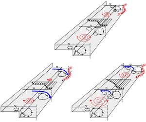
Figure 3. Detection of Kelvin–Helmholtz-type coherent structures using a dye tracer that is injected at $x^{\ast }=6.4$ for the cases of (a) $4~\text{l}~\text{s}^{-1}$ and (b) $20~\text{l}~\text{s}^{-1}$.

To visualize the presence of KHCSs in the flow, we have used a dye tracer (potassium permanganate). As shown in figure 3, this tracer was injected over the FP very near the interface, where large horizontal structures are expected to be generated. Two video cameras were used to get both a global view from the right-hand side of the flume and a top view perpendicular to water surface.

4.1 Depth-averaged velocity at the interface

Figures 5(a) and 5(b) respectively show the depth-averaged transverse and streamwise velocities along the MC/right-FP interface. The case of $8~\text{l}~\text{s}^{-1}$, which is uniform in terms of flow depth (figure 4), exhibits change in the depth-averaged streamwise velocity $U_{xd}$ along the whole measuring domain (figure 5b), reflecting the continuing development of the shear layer (§ 4.3). This development is accompanied with small negative values of transverse velocity $U_{yd}$, mostly along the upstream half of the flume (figure 5a). These negative $U_{yd}$-values correspond to a weak mass transfer from MC to FP, which may be caused by: (a) a small underestimation of the FP inflow required for equilibrium conditions with zero transverse mass exchange between MC and FP; or/and (b) the uniform distribution across the channel of the streamwise mean velocity at the outlet of each of the three inlet tanks (at $x^{\ast }=0$).

Introducing unbalanced partitioning of the water discharge in the inlet tanks leads to the emergence of transverse currents which magnitude grows with increasing imbalance and which spatial extent reaches the flume length (figure 5a). For the two extreme cases (0 and $20~\text{l}~\text{s}^{-1}$), the $U_{yd}$-values attain ${\approx}5\,\%$ and ${\approx}9\,\%$ of the $U_{xd}$-values, respectively.

Figure 5. Depth-averaged (a) transverse and (b) streamwise mean velocities, depth-averaged (c) transverse and (d) streamwise turbulence intensities, (e) depth-averaged transverse Reynolds shear stress and (f) transverse flux of streamwise momentum by the depth-averaged flow. Measurements are along the MC/right-FP interface for cases: $0~\text{l}~\text{s}^{-1}$ (▿); $4~\text{l}~\text{s}^{-1}$ (○); $8~\text{l}~\text{s}^{-1}$ ($\times$); $12~\text{l}~\text{s}^{-1}$ (▫); $16~\text{l}~\text{s}^{-1}$ (▵); and $20~\text{l}~\text{s}^{-1}$ (♢). The standard sampling errors in $U_{x}$, $U_{y}$, $\sqrt{\overline{u_{x}^{\prime 2}}}$, $\sqrt{\overline{u_{y}^{\prime 2}}}$ and $-\overline{u_{x}^{\prime }u_{y}^{\prime }}$ are around 1 %, 9 %, 3 %, 2 % and 10 %, respectively.

4.2 Transverse profiles of time-averaged streamwise velocity

Transverse profiles of local time-averaged streamwise velocity, $U_{x}$, for the reference (depth-uniform) flow are shown in figure 6(a). Measurements were taken at a fixed elevation $z^{\ast }=0.94$, i.e. at ${\approx}70\,\%$ of the FP flow depth $D_{f}^{u}$ from the FP bed. Similarly to Stocchino & Brocchini (Reference Stocchino and Brocchini2010) and Dupuis et al. (Reference Dupuis, Proust, Berni and Paquier2017b), the velocity scale used to normalize local time-averaged velocities (and turbulence quantities in the sequel) is the time-averaged streamwise velocity at the MC/FP interface, $U_{x,int}$. Note that: (i) Dupuis et al. (Reference Dupuis, Proust, Berni and Paquier2017a) found the depth-averaged value of $U_{x,int}$ to be very close to the convection velocity of the KHCSs that may populate the interfacial region; and (ii) the velocity scale $U_{x2}-U_{x1}$ used to normalize velocity data for free mixing layers is not sufficiently robust for our case as it attains very small values in some of our experiments (e.g. 16 and $20~\text{l}~\text{s}^{-1}$) and therefore the interface velocity is more appropriate for normalizations.

The time-averaged velocity profiles are monotonic with an inflection point near the interface where $y^{\ast }=1$. According to Nezu et al. (Reference Nezu, Onitsuka, Iketani, Seo, Singh and Sonu1999) and Stocchino & Brocchini (Reference Stocchino and Brocchini2010) who classified time-averaged velocity profiles for uniform flows depending on the $D_{r}$-value, the case of $8~\text{l}~\text{s}^{-1}$ belongs to the ‘shallow flow regime’, i.e. when $D_{r}\leqslant 0.37$ in Nezu et al. (Reference Nezu, Onitsuka, Iketani, Seo, Singh and Sonu1999) or $D_{r}\leqslant 0.33$ in Stocchino & Brocchini (Reference Stocchino and Brocchini2010) while in our case $D_{r}=0.21$. The monotonic velocity profiles at this flow regime are associated with large-scale vortical structures in the horizontal plane that rotate clockwise in the right-hand interfacial region (Stocchino & Brocchini Reference Stocchino and Brocchini2010). The location of the inflection point at $y^{\ast }\approx 1$, where the large-scale structures are generated, highlights the role played by a sudden change in topography on the generation of these structures (e.g. Soldini et al. Reference Soldini, Piattella, Mancinelli, Bernetti and Brocchini2004).

Figure 6. Transverse distributions of dimensionless (a) mean streamwise velocity, $U_{x}/U_{x,int}$, (b) transverse squared turbulence intensity, $\overline{u_{y}^{\prime 2}}/U_{x,int}^{2}$, and (c) transverse Reynolds shear stress, $-\overline{u_{x}^{\prime }u_{y}^{\prime }}/U_{x,int}^{2}$, all at elevation $z^{\ast }=0.94$ for the case of $8~\text{l}~\text{s}^{-1}$. The standard errors in $U_{x}$, $\overline{u_{y}^{\prime 2}}$ and $-\overline{u_{x}^{\prime }u_{y}^{\prime }}$ are around 1 %, 4 % and 10 %, respectively.

In the presence of transverse currents, the cross-flow distribution of streamwise mean velocity can be strongly modified, as shown in figure 7 for the cases of 0 and $20~\text{l}~\text{s}^{-1}$. In particular, the shear layer, defined using mean velocity distributions, is displaced in the direction of the transverse currents. For instance, with transverse currents towards MC ($20~\text{l}~\text{s}^{-1}$), the shear layer is nearly entirely shifted in the MC (figure 7d). This interplay between transverse currents and shear layer will be further described in the next section.

Figure 7. Transverse profiles of dimensionless time-averaged streamwise velocity, $U_{x}/U_{x,int}$, transverse squared turbulence intensity, $\overline{{u_{y}^{\prime }}^{2}}/U_{x,int}^{2}$, and transverse Reynolds shear stress, $-(\overline{u_{x}^{\prime }u_{y}^{\prime }})/U_{x,int}^{2}$, at various $x^{\ast }$-positions and at $z^{\ast }=0.91$ for the cases of (a–c) $0~\text{l}~\text{s}^{-1}$, and (d–f) $20~\text{l}~\text{s}^{-1}$. The standard errors in $U_{x}$, $\overline{u_{y}^{\prime 2}}$ and $-\overline{u_{x}^{\prime }u_{y}^{\prime }}$ are around 1 %, 4 % and 10 %, respectively.

4.3 Shear layer width

To illustrate the longitudinal evolution of the streamwise time-averaged flow, half the shear layer width, $\unicode[STIX]{x1D6FF}_{0}/2$, at a given $z^{\ast }$-elevation, is shown in figure 8. To quantify the transverse size of the shear layer we use the definition of van Prooijen, Battjes & Uijttewaal (Reference van Prooijen, Battjes and Uijttewaal2005),

(4.1)$$\begin{eqnarray}\unicode[STIX]{x1D6FF}_{0}=2(y_{75\,\%}-y_{25\,\%}),\end{eqnarray}$$

where $y_{25\,\%}$ corresponds to a location where $U_{x}(y_{25\,\%})=U_{x1}+0.25(U_{x2}-U_{x1})$ and $y_{75\,\%}$ is a location where $U_{x}(y_{75\,\%})=U_{x1}+0.75(U_{x2}-U_{x1})$. Here, $U_{x1}$ is the streamwise velocity averaged across the plateau region of $U_{x}=f(y^{\ast })$ over the right-hand FP, and $U_{x2}$ is the peak streamwise velocity in the MC.

The data for the reference case of $8~\text{l}~\text{s}^{-1}$ (figures 6 and 8) highlight three important differences from the unbounded plane free shear layer (see e.g. Champagne, Pao & Wygnanski Reference Champagne, Pao and Wygnanski1976; Oster & Wygnanski Reference Oster and Wygnanski1982): (i) the downstream linear growth of the shear layer is observed only in the MC while its transverse development over the FP is saturated at mid-length of the flume; (ii) the shear layer expands more rapidly on the high velocity side of the shear region compared to the low velocity side; and (iii) the position $y_{50\,\%}$ of the mean streamwise velocity $U_{x}(y_{50\,\%})=U_{x1}+0.5(U_{x2}-U_{x1})$ shifts away from the position of the inflection point ($y^{\ast }\approx 1$) into MC when moving downstream.

It should be noted that the asymmetry of the shear layer for uniform flows in compound open channels was recently highlighted and analysed by Dupuis et al. (Reference Dupuis, Proust, Berni and Paquier2017a). To interpret the differences (i) and (ii), we may recall the works of Chu & Babarutsi (Reference Chu and Babarutsi1988) and Uijttewaal & Booij (Reference Uijttewaal and Booij2000) on shallow mixing layers in non-compound open channels and assume that the transverse development of shear layer (horizontal) turbulence is constrained by the strong vertical flow confinement over the FP and that its expansion is stronger suppressed by the vertical bed-induced turbulence over the FP than in the MC at a given $z^{\ast }$-elevation. However, the analysis of the KHCSs is required to confirm or reject this hypothesis (as discussed in § 5).

Figure 8. Half shear layer width, $\unicode[STIX]{x1D6FF}_{0}/2$ (normalized by $B_{f}$), bounded by the transverse positions: $y_{25\,\%}$ (●); and $y_{75\,\%}$ (○). Position $y_{50\,\%}$ ($\times$) is also plotted. Measurements are at $z^{\ast }=0.94$ for the case of $8~\text{l}~\text{s}^{-1}$, and at $z^{\ast }=0.91$ for the other cases. Arrows indicate the direction of transverse currents.

In the presence of transverse currents, the data in figure 8 indicate that the shear layer is displaced in the direction of the transverse currents (as shown by arrows), with the case of $8~\text{l}~\text{s}^{-1}$ given as the reference. The effects of transverse currents on the shear layer are particularly noticeable at small $x^{\ast }$, e.g. at $x^{\ast }=4.4$, three quarters of the shear layer for the case of $4~\text{l}~\text{s}^{-1}$ is located over the FP while for the case of $16~\text{l}~\text{s}^{-1}$ three quarters of the shear layer is sited in the MC. This significant lateral displacement of the shear layer is caused by the high cross-flow momentum exchange via the transverse currents (as reflected in high values of $-\unicode[STIX]{x1D70C}U_{xd}U_{yd}$ in figure 5f). For the extreme cases of 0 and $20~\text{l}~\text{s}^{-1}$ (figure 5a), values of $-\unicode[STIX]{x1D70C}U_{xd}U_{yd}$ are even one order of magnitude higher than the depth-averaged Reynolds shear stresses (figure 5e).

Further downstream, the effects of transverse currents directed to the MC (12, 16 and $20~\text{l}~\text{s}^{-1}$) can still be seen along the whole measurement domain, as the shear layers remain mostly within the MC. With the transverse currents towards the FPs (0 and $4~\text{l}~\text{s}^{-1}$), the recovery of the shear layer over the FP to the depth-uniform case $8~\text{l}~\text{s}^{-1}$ appears to be faster compared to the opposite direction of the transverse currents (12, 16, $20~\text{l}~\text{s}^{-1}$), as observed at the downstream part of the flume (figure 8). The similar asymmetry in the relaxation towards uniformity (depending on the direction of transverse currents) was already noted in § 3 when considering streamwise profiles of the flow depth. The causes of this asymmetry will be analysed in § 7.

4.4 Turbulence statistics

For the depth-uniform reference case ($8~\text{l}~\text{s}^{-1}$), the spanwise profiles of normalized turbulence statistics are shown in figure 6. The transverse turbulence intensity $\overline{u_{y}^{\prime 2}}/U_{x,int}^{2}$ and Reynolds stress $-\overline{u_{x}^{\prime }u_{y}^{\prime }}/U_{x,int}^{2}$ rapidly evolve from $x^{\ast }=2.2$ to 10.2; then from $x^{\ast }=12.2$ to 16.8 only a very weak increase in $\overline{u_{y}^{\prime 2}}/U_{x,int}^{2}$ and $-\overline{u_{x}^{\prime }u_{y}^{\prime }}/U_{x,int}^{2}$ can be observed, mostly in the MC. This result is consistent with the streamwise evolution of the KHCSs along the flume, as will be demonstrated in § 5.

In the presence of transverse currents, the cross-flow profiles of normalized turbulence statistics are shown in figure 7 for cases 0 and $20~\text{l}~\text{s}^{-1}$. For both flow cases, at a given $x^{\ast }$-position, the lateral extent of the region of high turbulence intensities and Reynolds shear stresses matches well the shear layer width, defined in the previous section based on the mean velocity profiles. In particular, at the $x^{\ast }$-positions where transverse currents are significant (figure 5a), the same transverse displacement is observed for $-(\overline{u_{x}^{\prime }u_{y}^{\prime }})/U_{x,int}^{2}$, $\overline{{u_{y}^{\prime }}^{2}}/U_{x,int}^{2}$ and the streamwise mean velocity profiles. For instance, for $0~\text{l}~\text{s}^{-1}$ at $x^{\ast }=4.4$, the turbulence statistics (figure 7b,c) are mostly located over the FP, similar to the shear layer (figures 8 and 7a) while for $20~\text{l}~\text{s}^{-1}$, the high values of $-(\overline{u_{x}^{\prime }u_{y}^{\prime }})/U_{x,int}^{2}$ and $\overline{{u_{y}^{\prime }}^{2}}/U_{x,int}^{2}$ remain sited in the MC all along the measuring domain (figure 7e,f), as observed for the shear layer defined using mean velocities (figures 8 and 7d).

Another important feature to note is that at 16 and $20~\text{l}~\text{s}^{-1}$ the transverse Reynolds stresses at the MC–FP interface are very low within first five metres from the flume entrance (figure 5e), even though the difference $U_{x2}-U_{x1}$ is not zero (table 1). This difference from other cases is due to the absence of KHCS in this flow section, as will be shown in § 5 (figure 15).

4.5 Secondary currents

It should be noted from the start that the time-averaged transverse velocity, $U_{y}$, and vertical velocity, $U_{z}$, are small compared to the streamwise velocity and thus a potential misalignment of the ADV probe can have a strong impact on the measured values of $U_{y}$ and $U_{z}$ (e.g. Peltier et al. Reference Peltier, Rivière, Proust, Mignot, Paquier and Shiono2013b). The data of $U_{y}$ and $U_{z}$ were therefore corrected. For the spanwise component, we assumed that the cross-sectional average of $U_{y}$-values in the half-MC equals to zero for the depth-uniform flow case ($8~\text{l}~\text{s}^{-1}$) at $x^{\ast }=15.9$. This procedure resulted in a rotation around the vertical axis of a yaw angle $\unicode[STIX]{x1D703}_{z}=0.8^{\circ }$. The same procedure was not applied to the $U_{z}$-component, as this velocity could not be measured within 1 cm thick near-surface layer. For this component, we assumed that $U_{z}$ should tend towards zero close to the channel bed. Employment of this condition led to slight rotations around the lateral axis (e.g. a pitch angle $\unicode[STIX]{x1D703}_{y}\approx 2^{\circ }$ for cases 20 and $4~\text{l}~\text{s}^{-1}$ at $x^{\ast }=4.4$).

For case $8~\text{l}~\text{s}^{-1}$, the distributions of $U_{y}$ and $U_{z}$ in MC at various $y^{\ast }$-coordinates at $x^{\ast }=15.9$ (figure 9a) suggest the existence of two SC cells: a large cell caused by the anisotropy of the planform shear layer turbulence, and a smaller cell near the bottom at the MC corner induced by topography. The negative values of $U_{z}$ over the water column from $y^{\ast }=1.3$ to 1.5 indicate that the large cell extends over the entire flow depth in this region, as sketched in figure 9(c).

Figure 9. Uniform case ($8~\text{l}~\text{s}^{-1}$): (a) vertical distributions of the time-averaged transverse velocity, $U_{y}$, and vertical velocity, $U_{z}$, across a half-MC at $x^{\ast }=15.9$ (a horizontal dotted line at $z^{\ast }=0.8$ indicates the bank-full stage in MC); (b) transverse distribution of $U_{y}$ at $z^{\ast }=0.94$ at $x^{\ast }=4.2$, and longitudinally averaged values between $x^{\ast }=4.2$ and 16.8 (denoted $\langle U_{y}\rangle _{x}$); (c) cross-sectional sketch of the three SC cells at $x^{\ast }=15.9$ (upstream view). The standard sampling errors in $U_{y}$ and $U_{z}$ are approximately 9 % and 16 %, respectively.

For the same flow, two transverse profiles of $U_{y}$ (at elevation $z^{\ast }=0.94$) are shown in figure 9(b): data at $x^{\ast }=4.2$; and longitudinally averaged data $\langle U_{y}\rangle _{x}$ (average between $x^{\ast }=4.2$ and 16.8). First, the data in MC reveal that the development of the large SC cell is not fully established at $x^{\ast }=4.2$. Second, figure 9(b) indicates the existence of a persistent SC cell near the interface on the FP side, termed the ‘longitudinal FP vortex’ by Tominaga & Nezu (Reference Tominaga and Nezu1991). The $U_{y}$-distribution at $x^{\ast }=4.2$ within FP is very close to the streamwise-averaged profile, indicating that this vortex is already fully developed in the upstream part of the flow. Tominaga & Nezu (Reference Tominaga and Nezu1991) observed a similar vortical motion for a relative depth $D_{r}=0.5$ and for both rough and smooth FPs, for $D_{r}=0.75$ with smooth FPs, but not for $D_{r}=0.25$ and smooth FPs. They therefore concluded that SCs were more driven by the cross-sectional topography (i.e. by $D_{r}$) rather than by wall roughness. The present data with $D_{r}=0.2$ and rough FPs, which reveal a strong longitudinal vortex with ratio $U_{y}/U_{x}$ reaching 5 %, suggest that wall roughness stimulates the emergence of the FP longitudinal vortex even when $D_{r}$ becomes small.

Figure 10. Case $20~\text{l}~\text{s}^{-1}$: (a) vertical distributions of the time-averaged transverse velocity, $U_{y}$, and vertical velocity, $U_{z}$, across a half-MC at $x^{\ast }=4.4$; (b) transverse distribution of $U_{y}$ at $z^{\ast }=0.91$ and $x^{\ast }=2.4$, 4.4 and 8.4; (c) sketch of the SC pattern in the half-MC at $x^{\ast }=4.4$ (upstream view). The standard errors in $U_{y}$ and $U_{z}$ are around 9 % and 16 %, respectively.

Figure 11. Case $4~\text{l}~\text{s}^{-1}$: (a) vertical distributions of the time-averaged transverse velocity, $U_{y}$, and vertical velocity, $U_{z}$, at $x^{\ast }=4.4$; (b) transverse distributions of $U_{y}$ at elevation $z^{\ast }=0.91$ and at various $x^{\ast }$-positions; and (c) sketch of the SC patterns in the half-MC at $x^{\ast }=4.4$ (upstream view). The standard errors in $U_{y}$ and $U_{z}$ are around 9 % and 16 %, respectively.

In the presence of transverse currents towards MC, the SC pattern radically differs from that observed in uniform flow, as shown in figure 10(a) for case $20~\text{l}~\text{s}^{-1}$ at $x^{\ast }=4.4$, where the transverse currents are significant (figure 5a). The small SC cell revealed for $8~\text{l}~\text{s}^{-1}$ (figure 9c) does not emerge at the MC corner. A single SC cell spans over the whole water depth (figure 10a,c). This helical motion along $x^{\ast }$-axis is not related to shear layer turbulence, as KHCSs do not exist at this longitudinal position (figure 3b, and follow-up figures 14 and 15). This cell is most likely induced by the horizontal shearing between the upper mean flow region above the bank-full stage in the MC and the inbank mean flow in the MC. A similar pattern is also found for case $16~\text{l}~\text{s}^{-1}$ (not shown here). A horizontal-shearing-induced helical motion was first observed by Shiono & Muto (Reference Shiono and Muto1998) in compound meandering channels, then by Bousmar et al. (Reference Bousmar, Wilkin, Jacquemart and Zech2004) in compound channels with narrowing FPs and by Proust et al. (Reference Proust, Riviere, Bousmar, Paquier, Zech and Morel2006) in a compound channel with an abrupt FP contraction. In addition, figure 10(b) indicates that the longitudinal FP vortex observed in the reference depth-uniform flow (figure 9b,c), has vanished at $x^{\ast }=4.4$. The SCs across the channel at this position are therefore essentially controlled by the transverse currents directed towards the MC. On the other hand, the $U_{y}$-distribution further downstream at $x^{\ast }=8.4$ (figure 10b), with a local deficit in $U_{y}$-velocity near the interface on the FP side, indicates the initial stage of the longitudinal FP vortex development.

With transverse currents towards FP, the shapes of the SC cells are qualitatively comparable to those in the reference flow (figure 9). For case $4~\text{l}~\text{s}^{-1}$, vertical profiles of $U_{y}$ and $U_{z}$ at $x^{\ast }=4.4$ are shown in figure 11(a), and figure 11(b) displays transverse distributions of $U_{y}$ at $z^{\ast }=0.91$ and $x^{\ast }=2.4$, 4.4 and 8.4. From these two figures, we can infer the schematic patterns of the SC cells drawn in figure 11(c). First, water flowing in the lower part of the MC is moving upward and towards the FP (figure 11a). Very close to the interface on the MC side, the $U_{y}$-values are thus essentially negative from either side of the bank-full stage ($z^{\ast }=0.8$), highlighting the transverse net mass flux from MC to FP. Second, near the interface in the lower part of the MC, we can infer a small SC cell rotating anti-clockwise when looking upstream, like the corner cell of the uniform case (figure 9c). Third, when moving away from the interface into MC, a large SC cell rotates clockwise like the large cell of the uniform case (figure 9c). This cell seems to be bigger than the uniform flow cell, which would be consistent with the increase of the planform shear layer turbulence from $8$ to $4~\text{l}~\text{s}^{-1}$ (§ 5, figure 15). Last, the transverse profiles of $U_{y}$ at $z^{\ast }=0.91$ (figure 11b) show that the longitudinal FP vortex is fully developed at $x^{\ast }=8.4$ (compare figures 9b and 11b), although its emergence is already visible at the upstream locations $x^{\ast }=2.4$ and 4.4. A $U_{y}$-profile at $x^{\ast }=4.4$ measured near the FP bottom (not shown here) and showing some positive $U_{y}$-values near the interface on the FP side confirms the presence of the FP vortex at an early stage of the longitudinal flow development. We can thus conclude that a transverse mean flow from MC to FP occurred above the longitudinal FP vortex, as sketched in figure 11(c).

5.1 Detection using dye tracer

In a preliminary step, KHCSs in our study were detected with a coloured tracer, with an injection point at $x^{\ast }=6.4$ near the MC/right FP interface on the FP side (see figure 3 for the cases of $4~\text{l}~\text{s}^{-1}$ and $20~\text{l}~\text{s}^{-1}$). For $4~\text{l}~\text{s}^{-1}$, the signature of a strong Kelvin–Helmholtz instability downstream of $x^{\ast }=6.4$ is evident, as weak but noticeable ejections of slow-momentum fluid from FP towards the faster flow in the MC can be observed (figure 3a). Each ejection is followed by a strong sweep of high-momentum fluid deeply penetrating into the slower flow over the FP. For $20~\text{l}~\text{s}^{-1}$ (figure 3b), an instability from either side of the interface is still visible downstream of $x^{\ast }=6.4$, but its signature is less profound. The fluid ejection from FP to MC is fairly weak, though transverse currents from FP towards MC could have made it easier. This weaker instability cannot be ascribed to the shallowness effects, as observed for shallow mixing layers in non-compound open channels (e.g. Chu & Babarutsi Reference Chu and Babarutsi1988; Uijttewaal & Booij Reference Uijttewaal and Booij2000), since the flow depths for 4 and $20~\text{l}~\text{s}^{-1}$ at $x^{\ast }=6.4$ were $D_{f}=27.8~\text{mm}$ and 35.1 mm, respectively (vertical confinement is thus higher for $4~\text{l}~\text{s}^{-1}$ where KHCSs are stronger). Note also that the highlighted asymmetry in visualized mixing layers is consistent with the data from mean velocity distributions in figure 8.

5.2 Characteristic length scales

To investigate the longitudinal and transverse development of KHCSs, space–time correlations of velocity fluctuations were used, based on the two-point velocity measurements. The employed space–time correlation function is defined as:

(5.1)$$\begin{eqnarray}R_{ij}^{i}(x_{i},\unicode[STIX]{x1D716}_{i},\unicode[STIX]{x1D70F})=\frac{\overline{u_{i}^{\prime }(x_{i},t)u_{j}^{\prime }(x_{i}+\unicode[STIX]{x1D716}_{i},t+\unicode[STIX]{x1D70F})}}{\sqrt{\overline{u_{i}^{\prime 2}(x_{i})}\overline{u_{j}^{\prime 2}(x_{i}+\unicode[STIX]{x1D716}_{i})}}},\end{eqnarray}$$

where $u_{i}^{\prime }$ is fluctuation of the $i$th velocity component, $x_{i}$ is a spatial coordinate (i.e. $x$ or $y$), $\unicode[STIX]{x1D716}_{i}$ is spatial lag in the $x_{i}$-direction, $t$ is time and $\unicode[STIX]{x1D70F}$ is time lag.

The function $R_{ij}^{i}(x_{i},\unicode[STIX]{x1D716}_{i},\unicode[STIX]{x1D70F})$ defined by (5.1) depends on the location of the reference point where a measurement probe is fixed, with another probe moving away point by point. The reference point was always located at the interface, while the second probe was moving laterally in the MC or over the FP, or longitudinally along the interface downstream of the flume.

Figure 12(a) shows examples of spatial correlation function (with zero time lag) of the transverse velocity fluctuation, $u_{y}^{\prime }$, in the streamwise direction along the interface, for three downstream positions of the reference (fixed) upstream probe. An example of the correlation function of $u_{y}^{\prime }$ across the FP at $x^{\ast }=4.4$ is plotted in figure 12(b) (the shapes of transverse correlation functions at $x^{\ast }=8.4$, 12.4 and 16.4 are similar). Based on these spatial correlation functions, we shall define three characteristic length scales of the KHCSs to be used in our considerations. To reduce potential uncertainties due to the shape of the correlation functions (especially when the two probes are close to each other) and limited maximum lag, we do not use the conventional integral scales and instead define the characteristic scales of the KHCSs as spatial lags corresponding to a particular correlation level (e.g. O’Neill et al. Reference O’Neill, Nicolaides, Honnery and Soria2004; McDonough Reference McDonough2007).

The first characteristic scale is a streamwise scale along the interface, $\unicode[STIX]{x1D6FF}_{int}^{CS}$, which corresponds to the longitudinal distance between the upstream fixed probe and the downstream moving probe when $R_{yy}^{x}$ crosses zero for the second time (see $\unicode[STIX]{x1D6FF}_{int}^{CS}$ at $x^{\ast }=14.9$ in figure 12a). This scale corresponds, approximately, to the $3/4$ of the spacing between the dominant structures in the longitudinal direction. The factor of $3/4$ follows from the approximation of the streamwise correlation function as a periodic function so that second crossing corresponds to approximately $3/4$ of the dominant period in the signal. The second characteristic scale of KHCSs, $\unicode[STIX]{x1D6FF}_{f}^{CS}$, corresponds to the transverse distance from the interface to the $y^{\ast }$-value within FP where $R_{yy}^{y}$ reaches 0.05 (figure 12b). The correlation level of 0.05 is chosen as it represents a level below which the correlation is not distinguishable from zero. Note that this scale is approximately equal to $3L_{f}$ (5.2) if the correlation function is approximated by $\exp (-\unicode[STIX]{x1D716}_{y}/L_{f})$, with

(5.2)$$\begin{eqnarray}L_{f}=\int _{-\infty }^{0}R_{yy}^{y}\,\text{d}\unicode[STIX]{x1D716}_{y},\end{eqnarray}$$

where $L_{f}$ is an integral transverse scale. The exponential approximation of $R_{yy}^{y}$ is found to match data fairly well, as shown in figure 12(b) for the case of $8~\text{l}~\text{s}^{-1}$ at $x^{\ast }=4.4$ within the spatial separations for which the two probes do not have an influence on each other ($|\unicode[STIX]{x1D716}_{y}|\geqslant 0.2$, see § 2.4). The third characteristic scale of KHCSs, $\unicode[STIX]{x1D6FF}_{m}^{CS}$, is similar to $\unicode[STIX]{x1D6FF}_{f}^{CS}$ but defined within the MC. The total characteristic width of the KHCSs can thus be defined as a sum of MC-hand and FP-hand scales, i.e.

(5.3)$$\begin{eqnarray}\unicode[STIX]{x1D6FF}^{CS}=\unicode[STIX]{x1D6FF}_{f}^{CS}+\unicode[STIX]{x1D6FF}_{m}^{CS}.\end{eqnarray}$$

Figure 12. Spatial correlation functions of transverse velocity fluctuations, $u_{y}^{\prime }$, for the case of $8~\text{l}~\text{s}^{-1}$ at elevation $z^{\ast }=0.94$: (a) along the interface ($y^{\ast }=1$), the fixed probe measuring at the $x^{\ast }$-position (as shown in the legend); and (b) across the right-hand FP, the fixed probe measuring at $y^{\ast }=1$. Also displayed are the streamwise length scale of KHCSs, $\unicode[STIX]{x1D6FF}_{int}^{CS}$, at $x^{\ast }=14.9$, and spanwise length scale over the right-hand FP, $\unicode[STIX]{x1D6FF}_{f}^{CS}$, at $x^{\ast }=4.4$.

5.3 Mismatch between shear layer and KHCSs

In addition to the above three scales of KHCSs, we can also consider two length scales of the shear layer (based on mean velocity distribution) on either side of the MC/FP interface, following Dupuis et al. (Reference Dupuis, Proust, Berni and Paquier2017a,Reference Dupuis, Proust, Berni and Paquierb). Given the strong asymmetry of the compound open-channel shear layer compared to the conventional free shear layer, these authors have divided the shear layer width, $\unicode[STIX]{x1D6FF}$, into two parts on either side of the interface,

(5.4)$$\begin{eqnarray}\unicode[STIX]{x1D6FF}=\unicode[STIX]{x1D6FF}_{f}+\unicode[STIX]{x1D6FF}_{m},\end{eqnarray}$$

which are defined with

(5.5a)$$\begin{eqnarray}\displaystyle & \displaystyle U_{x}(y_{int}+\unicode[STIX]{x1D6FF}_{m}/2)=\frac{U_{x2}+U_{x,int}}{2}, & \displaystyle\end{eqnarray}$$

(5.5b)$$\begin{eqnarray}\displaystyle & \displaystyle U_{x}(y_{int}-\unicode[STIX]{x1D6FF}_{f}/2)=\frac{U_{x1}+U_{x,int}}{2}, & \displaystyle\end{eqnarray}$$

$y_{int}$

$\unicode[STIX]{x1D6FF}$

$\unicode[STIX]{x1D6FF}_{f}$

$\unicode[STIX]{x1D6FF}_{m}$

$(U_{x1}+U_{x2})/2$

We can now consider the simultaneous evolutions of $\unicode[STIX]{x1D6FF}_{f}$, $\unicode[STIX]{x1D6FF}_{m}$, $\unicode[STIX]{x1D6FF}_{f}^{CS}$, $\unicode[STIX]{x1D6FF}_{m}^{CS}$ and $\unicode[STIX]{x1D6FF}_{int}^{CS}$, which are first shown for the reference depth-uniform flow in figure 13. First, figure 13 highlights a noticeable decoupling of the time-averaged flow with KHCSs all along the flume, as $\unicode[STIX]{x1D6FF}_{m}\geqslant \unicode[STIX]{x1D6FF}_{f}$ while $\unicode[STIX]{x1D6FF}_{m}^{CS}\leqslant \unicode[STIX]{x1D6FF}_{f}^{CS}$. In addition, figure 13(c) indicates that, upstream, the growth rate of the structures is higher than that of the shear layer. Further downstream, the opposite trend is observed, and an equilibrium between time-averaged flow and KHCSs is eventually reached at the far end of the flume. Second, figure 13(b) shows that the transverse extent of the KHCSs is higher over the FP compared to the MC. The assumption that shallowness effects (bed-induced turbulence and flow confinement) on KHCSs are stronger in the FP than in the MC (made in § 4.3) thus is not supported by the data. The comparison with non-compound channel shear layers may not be too helpful, as there is no potential decay of destabilizing shear $U_{x1}-U_{x2}$ and shear layer turbulence when moving downstream in our case, owing to the presence of the persistent lateral change in topography, which enables the transverse turbulent momentum exchange to be self-sustained.

Figure 13. Case $8~\text{l}~\text{s}^{-1}$, elevation $z^{\ast }=0.94$: (a) shear layer widths based on mean velocity distribution in the MC, $\unicode[STIX]{x1D6FF}_{m}$, and over the FP, $\unicode[STIX]{x1D6FF}_{f}$; (b) characteristic scales of KHCSs in the MC, $\unicode[STIX]{x1D6FF}_{m}^{CS}$, in the FP, $\unicode[STIX]{x1D6FF}_{f}^{CS}$, and along the interface, $\unicode[STIX]{x1D6FF}_{int}^{CS}$; (c) ratios $\unicode[STIX]{x1D6FF}_{m}^{CS}/\unicode[STIX]{x1D6FF}_{m}$ and $\unicode[STIX]{x1D6FF}_{f}^{CS}/\unicode[STIX]{x1D6FF}_{f}$.

Figure 14. Non-uniform cases: (a–e) shear layer widths based on the mean velocity distributions in MC, $\unicode[STIX]{x1D6FF}_{m}$, and over FP, $\unicode[STIX]{x1D6FF}_{f}$; (f–j) characteristic scales of KHCSs in MC, $\unicode[STIX]{x1D6FF}_{m}^{CS}$, and in FP, $\unicode[STIX]{x1D6FF}_{f}^{CS}$.

For the non-uniform flows, the mismatch between the longitudinal developments of $\unicode[STIX]{x1D6FF}_{m}$ and $\unicode[STIX]{x1D6FF}_{m}^{CS}$ on the one hand, and between the developments of $\unicode[STIX]{x1D6FF}_{f}$ and $\unicode[STIX]{x1D6FF}_{f}^{CS}$ on the other hand, becomes far more visible (figure 14). It is most obvious for $20~\text{l}~\text{s}^{-1}$ where KHCSs deeply penetrate into the FP in the downstream half of the flume ($\unicode[STIX]{x1D6FF}_{f}^{CS}=0.8~\text{m}$ in the last measuring section), while $\unicode[STIX]{x1D6FF}_{f}\leqslant 0.05~\text{m}$ for all $x^{\ast }$-positions. In the MC, a different trend can be observed where the shear layer starts developing before the KHCS emergence. The increase in $\unicode[STIX]{x1D6FF}_{m}$ between $x^{\ast }=2.4$ and 4.4 (where $\unicode[STIX]{x1D6FF}_{m}^{CS}=0$) is essentially due to the mass and momentum transfers by the time-averaged transverse flow from the FP towards the MC. The same trends are visible for $16~\text{l}~\text{s}^{-1}$.

For $12~\text{l}~\text{s}^{-1}$, the ‘decorrelation’ between $\unicode[STIX]{x1D6FF}_{f}$ and $\unicode[STIX]{x1D6FF}_{f}^{CS}$ is still significant, as the shear layer is displaced in the MC by the transverse currents. In the MC, we may assume that KHCSs contribute to the shear layer development with a ratio $\unicode[STIX]{x1D6FF}_{m}^{CS}/\unicode[STIX]{x1D6FF}_{m}$ ranging from 3 to 2.5 in the second half of the flume, close to the values observed for the uniform case (figure 13c).

For 0 and $4~\text{l}~\text{s}^{-1}$, a noticeable difference with the previous cases can be observed. The FP flow is accelerated by the KHCSs but also by the time-averaged flow as high-momentum fluid from the MC is entering the FP (see the values of $-\unicode[STIX]{x1D70C}U_{xd}U_{yd}$ in figure 5f). Both the mean flow and the KHCSs therefore contribute to the increase in $\unicode[STIX]{x1D6FF}_{f}$, as also observed in diverging FPs (e.g. Proust et al. Reference Proust, Bousmar, Riviere, Paquier and Zech2010). The difference in the relaxation towards flow uniformity (depending on the direction of transverse currents) visible in figure 8 partly originates from noted trends in KHCS developments and the effect of the depth-averaged transverse mean flow (§ 7.2). Last, we can observe a spatial delay between the developments of KHCSs and shear layer near the flume entrance, similar to the uniform flow (figure 13c). Large KHCSs extend nearly over the entire FP width within the upstream part of the flume, which is not matched by the shear layer lateral extent.

It is important to notice that the KHCS length scale in MC, $\unicode[STIX]{x1D6FF}_{m}^{CS}$, can exceed the half-width of the MC (0.5 m). This feature is observed for both uniform (figure 13b) and non-uniform flows (figure 14f–h). The MC centreline is a symmetry axis where gradient $\text{d}U_{x}/\text{d}y$, time-averaged transverse flow and associated momentum transfer are zero. This results in a shear layer width in MC, $\unicode[STIX]{x1D6FF}_{m}$, always less than 0.5 m (figures 13 and 14). On the other hand, the MC centreline is not a barrier for the structures of the instantaneous velocity field, such as KHCSs, and dye tracer, which can cross $y^{\ast }=0.5$ intermittently, directed from one bank to another, resulting in $\unicode[STIX]{x1D6FF}_{m}^{CS}\geqslant 0.5~\text{m}$. Note that vortices wider than a half-width of MC were also observed by Stocchino & Brocchini (Reference Stocchino and Brocchini2010, figure 3). It is also worth highlighting at this point that $\unicode[STIX]{x1D6FF}_{m}^{CS}$ is a scale, not an actual size, and that this scale is three times larger than the integral transverse scale (as explained in § 5.2).

5.4 Effect of the dimensionless velocity shear on KHCSs

Figure 15. Characteristic scales of KHCSs at $z^{\ast }=0.94$ (a) in FP, $\unicode[STIX]{x1D6FF}_{f}^{CS}$, (b) in MC, $\unicode[STIX]{x1D6FF}_{m}^{CS}$, and (c) along the interface, $\unicode[STIX]{x1D6FF}_{int}^{CS}$, and (d) dimensionless shear $\unicode[STIX]{x1D706}$ (see (5.6)), for the cases of $0~\text{l}~\text{s}^{-1}$ (▿), $4~\text{l}~\text{s}^{-1}$ (○), $8~\text{l}~\text{s}^{-1}$ ($\times$), $12~\text{l}~\text{s}^{-1}$ (▫), $16~\text{l}~\text{s}^{-1}$ (▵) and $20~\text{l}~\text{s}^{-1}$ (♢).

The longitudinal developments of $\unicode[STIX]{x1D6FF}_{f}^{CS}$, $\unicode[STIX]{x1D6FF}_{m}^{CS}$ and $\unicode[STIX]{x1D6FF}_{int}^{CS}$ for all cases are grouped together in figure 15(a–c). The first important feature to note is a wide range of the characteristic scales of KHCSs at a given $x^{\ast }$-position across the flow cases. In particular, at the first measuring section the length scales systematically increase with increase in the destabilizing shear $U_{x2}-U_{x1}$ (table 1) or dimensionless shear $\unicode[STIX]{x1D706}$ (Brown & Roshko Reference Brown and Roshko1974),

(5.6)$$\begin{eqnarray}\unicode[STIX]{x1D706}=\frac{U_{x2}-U_{x1}}{U_{x2}+U_{x1}},\end{eqnarray}$$

which is plotted in figure 15(d). It is useful to mention at this point that the dimensionless shear $\unicode[STIX]{x1D706}$ can be physically interpreted in a number of ways. One of them is to consider $\unicode[STIX]{x1D706}$ as a measure of a ratio of the conventional vorticity scale $\unicode[STIX]{x1D6FF}_{\unicode[STIX]{x1D714}}=(U_{x2}-U_{x1})/(\text{d}U_{x}/\text{d}y)_{int}$ to the shear scale $\unicode[STIX]{x1D6FF}_{s}=U_{x,int}/(\text{d}U_{x}/\text{d}y)_{int}\approx 0.5(U_{x2}+U_{x1})/(\text{d}U_{x}/\text{d}y)_{int}$, i.e. $\unicode[STIX]{x1D706}=0.5\unicode[STIX]{x1D6FF}_{\unicode[STIX]{x1D714}}/\unicode[STIX]{x1D6FF}_{s}$. It can also be viewed as the square root of the ratio of the turbulence energy associated with KHCSs ($\propto (U_{x2}-U_{x1})^{2}$) to the energy associated with bed-friction depth-scale turbulence ($\propto (0.5(U_{x2}+U_{x1}))^{2}$). Interestingly, our data show that KHCS scales increase with reduction of the flow depth (i.e. with an increase in flow confinement) from $20$ to $0~\text{l}~\text{s}^{-1}$ (table 1), in contrast to observations for non-compound open channels mentioned earlier.

Second, KHCSs are observed along the whole measuring domain for 0, 4, 8 and $12~\text{l}~\text{s}^{-1}$, but not for 16 and $20~\text{l}~\text{s}^{-1}$. For these two cases, KHCSs are absent close to the flume entrance (at $x^{\ast }=2.4$), although neither destabilizing shear $U_{x2}-U_{x1}$ (table 1) nor dimensionless shear $\unicode[STIX]{x1D706}$ (figure 15d) are zero there.

The emergence of KHCSs is found to be related to the local (threshold) value of the dimensionless shear $\unicode[STIX]{x1D706}$ (or $\unicode[STIX]{x1D6FF}_{\unicode[STIX]{x1D714}}/\unicode[STIX]{x1D6FF}_{s}$). This result, based on two-point measurements, is fully consistent with earlier one-point measurements of Proust et al. (Reference Proust, Fernandes, Leal, Rivière and Peltier2017), who investigated 25 flow cases in two different open-channel flumes at three levels of vertical flow confinement. A dimensionless shear $\unicode[STIX]{x1D706}$ higher than 0.3 was found to be a necessary condition for the emergence and development of the KHCSs. Note that as $\unicode[STIX]{x1D706}$ is a monotonically decreasing function of velocity ratio $U_{x1}/U_{x2}$, the condition $\unicode[STIX]{x1D706}\geqslant 0.3$ is equivalent to $U_{x1}/U_{x2}\leqslant \approx 0.5$. No effect of flow confinement on the threshold value of $\unicode[STIX]{x1D706}$ was noted. In the present study (figure 15), no KHCS can be observed if $\unicode[STIX]{x1D706}<0.3$, in agreement with the previous findings of Proust et al. (Reference Proust, Fernandes, Leal, Rivière and Peltier2017). When the dimensionless shear reaches 0.3, KHCSs start emerging along the interface before expanding into MC and FP (see $\unicode[STIX]{x1D6FF}_{f}^{CS}$, $\unicode[STIX]{x1D6FF}_{m}^{CS}$ and $\unicode[STIX]{x1D6FF}_{int}^{CS}$ for 16 and $20~\text{l}~\text{s}^{-1}$, figure 15). This is also clearly seen in figure 3(b) for $20~\text{l}~\text{s}^{-1}$, where the instability starts developing longitudinally along the interface downstream of $x^{\ast }=6.4$ with a very small amplitude in the lateral direction (longitudinal oscillation without formation of spiral-shaped vortices, as sketched by Lesieur (Reference Lesieur2013, p. 50) for free mixing layers).

The conditions $\unicode[STIX]{x1D706}\geqslant 0.3$ and $U_{x1}/U_{x2}\leqslant \approx 0.5$ are also equivalent to,

(5.7)$$\begin{eqnarray}\unicode[STIX]{x1D6FF}_{\unicode[STIX]{x1D714}}\geqslant 0.6\unicode[STIX]{x1D6FF}_{s},\end{eqnarray}$$

demonstrating that KHCSs emerge once the vorticity strength at the inflection point (quantified with $\unicode[STIX]{x1D6FF}_{\unicode[STIX]{x1D714}}$) exceeds the effect of velocity shear (quantified with $\unicode[STIX]{x1D6FF}_{s}$ that characterizes interplay between mean energy diffusion and conversion of mean energy to turbulence). Recalling that the dimensionless shear $\unicode[STIX]{x1D706}$ represents the square root of the ratio of the turbulence energy associated with KHCSs to the energy associated with bed-friction depth-scale turbulence, one may argue that KHCSs start to emerge once large-scale energy becomes dominant in the velocity spectrum.

The criterion of $\unicode[STIX]{x1D706}\geqslant 0.3$ for the emergence of KHCSs was recently found to be confirmed in the experiments of Caroppi et al. (Reference Caroppi, Västilä, Järvelä, Rowinski and Giugni2019) that focused on water–vegetation interfaces in open-channel flow. On the other hand, the experiments of Akutina et al. (Reference Akutina, Eiff, Moulin and Rouzes2019) show that, in the case of a lateral bed-roughness variation in shallow open-channel flow with very low submergence, this criterion is no longer valid. This might be due to the effect of the bed-induced strong turbulence generated at the top of the roughness elements that would prevent emergence of the transverse turbulent motions in the case of a very low submergence of the roughness elements.

Third, figure 15(a–c) highlights for all flow cases an increase of the KHCS size in the transverse direction (both in MC and FP) and in the longitudinal direction, when moving downstream. In MC, the development rate of KHCSs does not seem to be sensitive to the magnitude and direction of transverse currents, as the growth rate $\text{d}(\unicode[STIX]{x1D6FF}_{m}^{CS})/\text{d}x$ does not significantly change from one case to another. Over the FP, the evolution of $\unicode[STIX]{x1D6FF}_{f}^{CS}$ appears to be more controlled by the location (downstream position $x^{\ast }$) where KHCSs emerge, i.e. where $\unicode[STIX]{x1D706}$ exceeds 0.3. The same applies for the growth of $\unicode[STIX]{x1D6FF}_{int}^{CS}$ along $x^{\ast }$. We can thus conclude that, unlike the shear layer, KHCSs are relatively weakly influenced by the transverse currents.

5.5 KHCSs and power density spectra of velocity fluctuations

Figure 16. Power density $S_{yy}$ of transverse velocity fluctuations $u_{y}^{\prime }$, as a function of wavenumber $k$, along the interface at elevation $z^{\ast }=0.91$ for the cases of 4, 8 and $20~\text{l}~\text{s}^{-1}$.

In addition to using coloured tracer and two-point velocity measurements to detect KHCSs, we also relied on power density spectra of velocity fluctuations. Figure 16 shows the power density $S_{yy}$ of the transverse velocity fluctuation $u_{y}^{\prime }$ as a function of wavenumber $k$ along the interface, for three flow cases. The wavenumber spectra are obtained from the frequency spectra assuming the applicability of the frozen turbulence hypothesis and using local time-averaged velocity as a convection velocity (with $k=2\unicode[STIX]{x03C0}f/U_{x}$ and $f$ $=$ frequency). The spectral evolution is characterized by the appearance of a sharp bump at large scales, which is then flanked by a $k^{-3}$ spectrum (on the right-hand side of the bump) when moving downstream. A similar spectral behaviour was first observed in 2-D turbulence inside a box, in the so-called condensation regime in which the system boundaries impose the peak vorticity value (see e.g. Tabeling Reference Tabeling2002, figure 56). We may speculate that the $k^{-3}$ scaling range in the observed spectra may reflect an enstrophy cascade (e.g. in freely decaying turbulence the theory of Kraichnan (Reference Kraichnan1967) and Batchelor (Reference Batchelor1969) predicted an energy spectrum in the form $E(k)\approx t^{-2}k^{-3}$).

In the present case, instead of a turbulence decay, we observe a growth of the $k^{-3}$ spectrum when moving downstream, as the shear layer turbulence is self-sustained by the lateral change in topography. The wavenumber corresponding to the sharp bump is most likely related to the streamwise length scale of the KHCSs, $\unicode[STIX]{x1D6FF}_{int}^{CS}$. For instance, for $8~\text{l}~\text{s}^{-1}$, an equilibrium state is reached with an energy peak at $k\approx 3~\text{rad}~\text{m}^{-1}$, i.e. with a wavelength of approximately 2 m, which is consistent with $\unicode[STIX]{x1D6FF}_{int}=1.5~\text{m}$ ($3/4$ of the distance between two vortex cores) at $x^{\ast }=15$ in figure 15(c).

The present experimental data also demonstrate that the appearance of the local peak of $S_{yy}$ within the intermediate range of wavenumbers (figure 16) always corresponds to the emergence of KHCSs. For instance, for $20~\text{l}~\text{s}^{-1}$, KHCSs start growing downstream at $x^{\ast }=6.4$ (figures 3b and 15c), while a small local peak in $S_{yy}$ appears between $x^{\ast }=6.2$ and 7.2 (figure 16). For 4 and $8~\text{l}~\text{s}^{-1}$, the local peak in $S_{yy}$ is visible at $x^{\ast }=1.2$ being consistent with the early emergence of KHCSs noted in the previous section (figure 15).

The power density spectra thus enable us to detect both the location of the emergence of KHCSs and the location where these structures become fully developed. For 4 and $8~\text{l}~\text{s}^{-1}$, a noticeable range of $k^{-3}$ can be observed already at $x^{\ast }\geqslant 2.2$, consistent with the results for the characteristic scales (figure 15), since the KHCSs are already very well developed in the upper part of the flume for these flows. At the interface, this results in high values of the transverse Reynolds shear stress, transverse and longitudinal turbulence intensities, as shown in figures 5(c), 5(d) and 5(e), respectively. The spectra in figure 16 indicate that a fairly long distance can separate the locations of emergence and full development with fully established $-3$ scaling range; e.g. for 4 and $8~\text{l}~\text{s}^{-1}$ (figure 16), these locations are respectively located at $x^{\ast }=1.2$ and 12.2, while for $12~\text{l}~\text{s}^{-1}$ (not shown here) at $x^{\ast }=2.2$ and $x^{\ast }=11.2$. For $20~\text{l}~\text{s}^{-1}$, the $k^{-3}$ spectrum is hardly visible even at $x^{\ast }=16.9$, owing to the late emergence of the KHCS (at $x^{\ast }\approx 6$).

Finally, it is worth mentioning that the spectra with a distinct bump and associated $-3$ $k$-range have been observed in open-channel flows for various contexts, in which quasi-2-D turbulence co-exists with 3-D turbulence. This was observed e.g. by Dracos, Giger & Jirka (Reference Dracos, Giger and Jirka1992) in shallow turbulent jets, by Uijttewaal & Booij (Reference Uijttewaal and Booij2000) in mixing layers in non-compound open-channel flows and by Stocchino & Brocchini (Reference Stocchino and Brocchini2010) and Proust et al. (Reference Proust, Fernandes, Leal, Rivière and Peltier2017) in compound open-channel flows. However, the solid link between the $k^{-3}$ spectrum of pure 2-D turbulence (without vortex stretching, based on 2-D Navier–Stokes equations) and the $k^{-3}$ spectra observed in quasi-2-D turbulence has not been yet fully established theoretically.

6.1 Uniform flow

It is currently widely accepted that the flow structure in straight uniform compound channels represents an interplay of the dynamic effects due to velocity shear in the transverse and vertical directions, involving at least three momentum transfer mechanisms: (i) topography-induced SCs which are time-averaged streamwise helical motions; (ii) planform (or horizontal) turbulence, which is typically manifested as large coherent structures (KHCSs) emerging as a result of Kelvin–Helmholtz instability due to the inflection point in the transverse velocity profile at the MC/FP interface; and (iii) bed-generated turbulence that shares (at least conceptually) many features with that observed in boundary layers and pipes (e.g. Nezu et al. Reference Nezu, Onitsuka, Iketani, Seo, Singh and Sonu1999; Ikeda & McEwan Reference Ikeda and McEwan2009).

In conventional uniform open-channel flow with rectangular cross-section, the bed-generated turbulence may consist of large-scale motions (up to 3–4 flow depths long) and very-large-scale motions (up to 50 flow depths long or even longer), as has been highlighted by Adrian & Marusic (Reference Adrian and Marusic2012) and recently demonstrated in high-precision experiments by Cameron et al. (Reference Cameron, Nikora and Stewart2017). The data for this flow type show that VLSMs contributions to the total turbulence energy and turbulent shear stresses may reach up to 50 % (Cameron et al. Reference Cameron, Nikora and Stewart2017; Cameron, Nikora & Marusic Reference Cameron, Nikora and Marusic2019) and, thus, these motions should be considered as a dominant flow feature. It was also shown that open-channel VLSMs play critical roles in sediment dynamics and mixing (Cameron et al. Reference Cameron, Nikora and Marusic2019). The interactions of VLSMs with other flow features such as SCs and/or planform turbulence (e.g. KHCSs) remain unclear. Indeed, transverse flow heterogeneity due to the roughness change or topographical change may affect the appearance and strength of VLSMs, as has been recently shown for the case of a rectangular channel with a bed covered by streamwise ridges (Zampiron Reference Zampiron2019; Zampiron, Cameron & Nikora Reference Zampiron, Cameron and Nikora2019). At spanwise spacing between ridges less than two flow depths the VLSMs are completely suppressed, presumably by strong SCs induced by the ridges. Although SCs and VLSMs share some common features such as helical motion patterns, there are some significant differences. On the one hand, VLSMs are represented by pairs of instantaneous meandering counter-rotating helical motions which are typically not seen in the time-averaged velocity fields. The SCs, in turn, do not need VLSMs to exist as SCs are generated by the action of turbulence heterogeneity and anisotropy.

There has been no information reported regarding emergence and significance of VLSMs in straight compound channels and thus our long-term (7 h) velocity measurements may provide some preliminary insights. To identify the existence of VLSMs in our experiments we used the pre-multiplied one-dimensional wavenumber spectra of streamwise velocity fluctuations that proved to be the tool of choice for this task (e.g. Kim & Adrian Reference Kim and Adrian1999; Hutchins & Marusic Reference Hutchins and Marusic2007; Cameron et al. Reference Cameron, Nikora and Stewart2017). As we measured velocity time series at fixed spatial locations, the obtained frequency spectra have been transformed into wavenumber spectra by employing Taylor’s frozen turbulence hypothesis with the local time-averaged velocity as the convection velocity.

Before discussing the pre-multiplied spectra we would like to mention that, for VLSMs to be observed in a laboratory flume, one needs a sufficient development length for them to emerge and fully establish. Considering conventional open-channel flow with rectangular cross-section, Zampiron (Reference Zampiron2019) has recently demonstrated that the minimum flow lengths required for the bulk statistics (mean velocity, variance, skewness and kurtosis), SCs and LSMs to fully establish need to be between 50 and 70 flow depths. The development distance for VLSMs appeared to be even longer. These results should be treated as suggestive only as they are likely to depend on specific experimental conditions such as flow aspect ratio, relative submergence, roughness geometry, channel shape and other parameters. Nevertheless, using Zampiron’s (Reference Zampiron2019) values as indicators we can assess the stage of the flow development in terms of LSM and VLSM for all three locations of long-term measurements ($x^{\ast }=4.4$, 8.2 and 15.9). Over FP, the closest measuring location (4.4 m) is approximately 145 flow depths from the flume entrance and thus we could expect that the flow is already fully developed there, if the potential effects of the transverse shear layer and KHCSs are excluded from consideration. Over MC, however, the situation is different: Zampiron’s (Reference Zampiron, Cameron and Nikora2019) conditions would be reasonably met only at the downstream measurement location at $x^{\ast }=15.9$ which is equivalent to 106 $x/D_{m}$, and probably at $x^{\ast }=8.2$ that corresponds to 55 $x/D_{m}$. Our experimental data for compound channel flows, however, do not support these expectations.

Figure 17 shows pre-multiplied spectra of streamwise velocity for all locations of long-term measurements (left-hand column is for FP and right-hand column is for MC). The smallest scales shown in these plots are defined by the size of the ADV sampling volume and its effect on the recorded velocities. Starting with MC, we first note that at the upstream location ($x^{\ast }=4.4$, $x/D_{m}=30$) the pre-multiplied spectrum exhibits a shape typical for the conventional flow in a rectangular channel (Cameron et al. Reference Cameron, Nikora and Stewart2017), i.e. it includes two ‘hills’ that most likely reflect the presence of LSMs (with wavelength $\unicode[STIX]{x1D706}_{0}\approx 1.6D_{m}$) and VLSMs (with $\unicode[STIX]{x1D706}_{0}\approx 18D_{m}$), figure 17(b), right-hand plot. This comes as a surprise bearing in mind a relatively short distance from the flume entrance ($x/D_{m}=30$), which is appreciably less than the development lengths of 50 to 70 flow depths in a conventional rectangular flume (Zampiron Reference Zampiron2019). A possible explanation of this discrepancy may relate to the use of the flow depth $D_{m}$ as a scale, which may not be appropriate for our experimental set up. An alternative scaling of the streamwise coordinate with the distance of the measurement point from the bed gives a relative distance from the flume entrance around 150, which seems sufficient for the emergence of VLSMs. The pre-multiplied spectrum for the transverse velocity component does not show a peak at $\unicode[STIX]{x1D706}_{0}\approx 18D_{m}$ while the coherence function between streamwise and spanwise velocity components do not reveal any correlations at the scales of LSMs ($\unicode[STIX]{x1D706}_{0}\approx 1.6D_{m}$) and VLSMs ($\unicode[STIX]{x1D706}_{0}\approx 18D_{m}$). These observations are consistent with Cameron et al. (Reference Cameron, Nikora and Stewart2017) for a conventional open-channel flow and thus they exclude potential relation of the spectral hills to KHCSs or other transverse shear layer effects. Moving downstream to $x/D_{m}=55$, the spectrum changes its shape, with the LSM hill growing and moving towards larger scales while the VLSM hill ‘dissolving’. At the most downstream location ($x/D_{m}=106$), the spectrum completely losses its bi-modal shape, transforming in a bell-shaped spectrum with a maximum at 4–5 flow depths. The observed downstream evolution of the pre-multiplied spectrum most likely reflects combined dynamic effects of the transverse shear layer, SCs and KHCSs. The data suggest that these flow features were insufficiently developed in the near-bed region of MC at $x^{\ast }=4.4$ allowing emergence of both LSMs and VLSMs at this location. However, further downstream their effects become sufficiently strong to suppress VLSMs, similar to the effect of SCs that suppressed VLSMs in the study of Zampiron et al. (Reference Zampiron, Cameron and Nikora2019).

Figure 17. One-dimensional pre-multiplied spectra of streamwise velocity fluctuations for flow cases: $4~\text{l}~\text{s}^{-1}$ (a); $8~\text{l}~\text{s}^{-1}$ (b); and $16~\text{l}~\text{s}^{-1}$ (c). $\unicode[STIX]{x1D706}_{0}$ is the wavelength of a spectral component; $\mathit{Var}\;u_{x}$ is the variance of the streamwise velocity.

Turning to FP, we note no visible LSM hills within the smaller scale range of the pre-multiplied spectra of streamwise velocity at all three studied locations (figure 17b, left-hand plot). Their absence is probably due to the mutual effects of the measurement noise and insufficient spatial resolution as the ADV sampling volume is comparable to the FP flow depth. Focusing on the spectrum at larger scales we note that, although at $x^{\ast }=4.4$ there is no visible spectral hill, it does appear at $x^{\ast }=8.2$ (around $\unicode[STIX]{x1D706}_{0}/D_{f}=40$), becoming a dominant spectral feature at $x^{\ast }=15.9$ (around $\unicode[STIX]{x1D706}_{0}/D_{f}=50$). The pre-multiplied spectra of the transverse velocity exhibit similar hills at the same wavelengths, which combined with the high coherence between streamwise and transverse velocities at these wavelengths (not shown here) suggest that their origin relates to the KHCSs that introduce strong periodicity in both streamwise and spanwise velocities over FP. The wavelengths $\unicode[STIX]{x1D706}_{0}/D_{f}=40$ (at $x^{\ast }=8.2$) and $\unicode[STIX]{x1D706}_{0}/D_{f}=50$ (at $x^{\ast }=15.9$) are in complete agreement with the correlation lengths $\unicode[STIX]{x1D6FF}_{int}^{CS}$ shown in figures 13(b) and 15(c) (recall that $\unicode[STIX]{x1D6FF}_{int}^{CS}$ corresponds to 0.75 of the dominant length scale, § 5.2).

Overall, the data for the uniform flow case ($8~\text{l}~\text{s}^{-1}$) suggest that in the initial development of KHCSs, SCs, LSMs and VLSMs in MC, the latter two appear to be fairly competitive but then they are quickly suppressed by the effects of either the transverse shear layer, KHCSs or SCs or their combined work. At the same time, it seems that within FP the effects of KHCSs became already dominant at $x^{\ast }=4.4$ suppressing the conditions allowing VLSMs to form. The dominating effect of KHCSs is likely supplemented by the artificial grass on the FP bed that could help to prevent emergence of VLSMs. The data indicate that the transverse shear layer, KHCSs and SCs become the most dominant features of the flow dynamics shortly after flow enters the flume.

6.2 Effects of the transverse currents

The effects of the transverse currents on LSMs and VLSMs within MC and FP can be seen in figures 17(a) ($4~\text{l}~\text{s}^{-1}$) and 17(c) ($16~\text{l}~\text{s}^{-1}$). Compared to the benchmark case of $8~\text{l}~\text{s}^{-1}$ (figure 17b) discussed in § 6.1, the pre-multiplied spectra in MC for both 4 and $16~\text{l}~\text{s}^{-1}$ appear to be very similar in shape and magnitudes. This observation suggests that near-bed turbulence and its evolution along the flow are only weakly (if at all) influenced by the transverse currents. The situation within FP is dramatically different. As in the $8~\text{l}~\text{s}^{-1}$ case, no signatures of VLSMs emerge in 4 and $16~\text{l}~\text{s}^{-1}$ cases, with their pre-multiplied spectra nevertheless being significantly different. The spectra for the case $4~\text{l}~\text{s}^{-1}$ exhibit significant hills, associated with KHCSs, at all measurement locations, with their wavelengths and magnitudes increasing downstream (figure 17a, left-hand plot). This picture and hill wavelengths are fully consistent with the findings for KHCSs outlined in §§ 5.3 and 5.4 (figures 14 and 15). In contrast, the case $16~\text{l}~\text{s}^{-1}$ is characterized by very weak signatures of KHCSs, which spectral signature becoming obvious only at $x^{\ast }=15.9$. This observation is also in full agreement with the findings reported in §§ 5.3 and 5.4 (figures 14 and 15). Both cases (4 and $16~\text{l}~\text{s}^{-1}$) do not show signs of VLSMs within FP, similar to $8~\text{l}~\text{s}^{-1}$ case.

7.1 Transverse exchange of streamwise momentum

In the presence of transverse currents, the time- and depth-averaged transverse exchange of streamwise momentum $\unicode[STIX]{x1D70F}_{tot}$ can be split into three components (e.g. Proust et al. Reference Proust, Fernandes, Peltier, Leal, Rivière and Cardoso2013),

(7.1)$$\begin{eqnarray}\unicode[STIX]{x1D70F}_{tot}=\overline{\frac{1}{D}\int _{0}^{D}-\unicode[STIX]{x1D70C}u_{x}u_{y}\,\text{d}z}=-\unicode[STIX]{x1D70C}(\overline{u_{x}^{\prime }u_{y}^{\prime }})_{d}-\unicode[STIX]{x1D70C}U_{xd}U_{yd}-\unicode[STIX]{x1D70C}[U_{x}(U_{y}-U_{yd})]_{d},\end{eqnarray}$$

where $u_{i}$ is the local instantaneous velocity component. Equation (7.1) is based on the decomposition of $u_{i}$ into three components: (i) time- and depth-averaged velocity $U_{id}$, (ii) deviation of the local time-averaged velocity from its depth-averaged counterpart and (iii) turbulent fluctuation $u_{i}^{\prime }$. Equation (7.1) explicitly shows that the total transverse exchange of momentum between MC and FP is driven by three key mechanisms: (i) transverse Reynolds stresses ($-\unicode[STIX]{x1D70C}(\overline{u_{x}^{\prime }u_{y}^{\prime }})_{d}$); (ii) transverse currents ($-\unicode[STIX]{x1D70C}U_{xd}U_{yd}$); and (iii) SCs ($-\unicode[STIX]{x1D70C}[U_{x}(U_{y}-U_{yd})]_{d}$).

Figure 18. Contributions of shear layer (planform) turbulence ($-\unicode[STIX]{x1D70C}(\overline{u_{x}^{\prime }u_{y}^{\prime }})_{d}$), transverse currents ($-\unicode[STIX]{x1D70C}U_{xd}U_{yd}$) and secondary currents ($-\unicode[STIX]{x1D70C}[U_{x}(U_{y}-U_{yd})]_{d}$) to the total depth-averaged momentum exchange $\unicode[STIX]{x1D70F}_{tot}$ (i.e. terms of (7.1)). Measurements are taken at the interface.

Figure 18 illustrates the relative contributions of these three key mechanisms at the interface. For all flow cases, shear layer (planform) turbulence and transverse currents have similar magnitudes in the depth-averaged momentum exchange, while the effect of SCs is negligible, consistent with the previous studies (e.g. van Prooijen et al. Reference van Prooijen, Battjes and Uijttewaal2005; Dupuis et al. Reference Dupuis, Proust, Berni and Paquier2017a). For the depth-uniform flow case $8~\text{l}~\text{s}^{-1}$, it should be noted that the contribution of $-\unicode[STIX]{x1D70C}U_{xd}U_{yd}$ is non-zero in the first half of the flume, due to the shear layer development. With transverse currents towards FPs (0 and $4~\text{l}~\text{s}^{-1}$), the momentum fluxes by the transverse Reynolds stresses and by the transverse currents have the same sign, both contributing to the FP flow acceleration and the hastened recovery to flow uniformity (figure 8). In contrast, with transverse currents towards MC (12, 16 and $20~\text{l}~\text{s}^{-1}$), the two mechanisms act against each other.

The transverse distributions of the three contributions to the depth-averaged transverse exchange of streamwise momentum in the MC are reported in figure 19(a) for the two extreme flow cases (20 and $0~\text{l}~\text{s}^{-1}$) at $x^{\ast }=4.4$ and 15.9. At both $x^{\ast }$-positions, the contributions of shear layer (planform) turbulence and SCs are of the same order of magnitude. Focusing on the upstream part of the flow, the transverse currents provide the predominant contribution to the spanwise momentum exchange, irrespective of the flow direction (from MC to FP or vice versa). In addition, figure 19(a) shows that $-\unicode[STIX]{x1D70C}U_{xd}U_{yd}$ and $-\unicode[STIX]{x1D70C}(\overline{u_{x}^{\prime }u_{y}^{\prime }})_{d}$ have the same sign for $0~\text{l}~\text{s}^{-1}$, both contributing to the deceleration of the MC flow, while these two terms are of opposite sign for $20~\text{l}~\text{s}^{-1}$.

Some examples of vertical distributions of the local momentum exchange terms by shear layer turbulence and SCs in the MC at $y^{\ast }=1.06$ are shown in figure 19(b). These distributions highlight the significance of the SCs in the local transverse exchange of momentum which may well exceed the contribution of the Reynolds stresses. However, the vertical integrals of the SC contributions are small compared to the action of transverse turbulence and can be negligible compared to the action of transverse currents, as highlighted above in figure 19(a).

Figure 19. (a) Transverse distributions of depth-averaged momentum fluxes by the transverse currents, $-\unicode[STIX]{x1D70C}U_{xd}U_{yd}$, by the shear layer turbulence, $-\unicode[STIX]{x1D70C}(\overline{u_{x}^{\prime }u_{y}^{\prime }})_{d}$, and by the SCs, $-\unicode[STIX]{x1D70C}[U_{x}(U_{y}-U_{yd})]_{d}$, for $20~\text{l}~\text{s}^{-1}$ (♢) and $0~\text{l}~\text{s}^{-1}$ (▿). (b) Vertical distributions of $-\unicode[STIX]{x1D70C}\overline{u_{x}^{\prime }u_{y}^{\prime }}$ and $-\unicode[STIX]{x1D70C}U_{x}(U_{y}-U_{yd})$ at $y^{\ast }=1.06$ for 0, 20 and $8~\text{l}~\text{s}^{-1}$.

Last, figure 20 shows the effect of the lateral momentum exchange on the cross-sectional distribution of the time-averaged velocity $U_{x}$ in MC for 0 and $20~\text{l}~\text{s}^{-1}$ at $x^{\ast }=8.2$ (with normalization by the peak velocity). For $20~\text{l}~\text{s}^{-1}$, the deceleration of the MC flow is noticeable near the MC–FP interface in the upper flow region, owing to the very high values of the flux $-\unicode[STIX]{x1D70C}U_{xd}U_{yd}$ upstream at $x^{\ast }=4.4$ (figure 19a). Slower water (mean flow) entering a faster flow in MC are responsible for this local decrease in velocity $U_{x}$. In contrast, for $0~\text{l}~\text{s}^{-1}$, as water is leaving the MC near the interface in the upper flow region, this decrease in $U_{x}$ is no more visible.

Figure 20. Cross-sectional distributions of the time-averaged streamwise velocity, $U_{x}$, normalized by the peak velocity, $U_{x,max}$, across a half-MC at $x^{\ast }=8.2$: (a) $20~\text{l}~\text{s}^{-1}$; (b) $0~\text{l}~\text{s}^{-1}$.

7.2 Relaxation towards flow uniformity

The plots in figures 18 and 19 have demonstrated that, in both MC and FP, the two key mechanisms of streamwise momentum exchanges act in the same direction for transverse currents directed towards FP, and act against each other for transverse currents directed towards MC. Indeed, with transverse currents towards the FP (0 and $4~\text{l}~\text{s}^{-1}$), the transverse fluxes of streamwise momentum by the mean flow and by the KHCSs have the same sign over the FP (figure 18) and are two key mechanisms of momentum gain for the FP flow, while in the MC, these two fluxes always lead to the momentum reduction (figure 19). This results in a hastened development of the shear layer (figure 8). With transverse currents towards the MC (12, 16 and $20~\text{l}~\text{s}^{-1}$), the KHCSs still serve as a mechanism of momentum supply to FP (figure 18), but the transverse flux of streamwise momentum by the mean flow represents momentum (and mass) loss. In MC, the transverse fluxes of streamwise momentum by transverse currents and KHCSs are also of opposite signs. As the two mechanisms of momentum transfer act in the opposite directions in both sub-sections, the development of the shear layer is delayed (figure 8).

The asymmetry in the relaxation towards flow uniformity (depending on the transverse currents direction) is also noticeable when focusing on the turbulence statistics. For instance, at the MC/FP interface (figure 5), the depth-averaged transverse turbulence intensity and transverse Reynolds stress for $0~\text{l}~\text{s}^{-1}$ are closer to the uniform flow values ($8~\text{l}~\text{s}^{-1}$) than the corresponding values for $16~\text{l}~\text{s}^{-1}$. The same trends hold when comparing $4$ to $12~\text{l}~\text{s}^{-1}$, with $8~\text{l}~\text{s}^{-1}$ as a reference flow.

Figure 21. Transverse profiles of dimensionless (a) mean streamwise velocity, $U_{x}/U_{x,int}$, (b) transverse turbulence intensity, $\overline{u_{y}^{\prime ^{2}}}/U_{x,int}^{2}$, and (c) transverse Reynolds shear stress, $-(\overline{u_{x}^{\prime }u_{y}^{\prime }})/U_{x,int}^{2}$, at $x^{\ast }=16.4$ and $z^{\ast }=0.91$ for cases $4~\text{l}~\text{s}^{-1}$ (○), $8~\text{l}~\text{s}^{-1}$ ($\times$), $12~\text{l}~\text{s}^{-1}$ (▫) and $16~\text{l}~\text{s}^{-1}$ (▵). The standard errors in $U_{x}$, $\overline{u_{y}^{\prime ^{2}}}$ and $-(\overline{u_{x}^{\prime }u_{y}^{\prime }})$, are approximately 1 %, 4 % and 10 %.

Figure 22. Vertical distributions of the time-averaged transverse velocity, $U_{y}$, at $y^{\ast }=1.06$ (in MC) and $x^{\ast }=15.9$, for cases: $0~\text{l}~\text{s}^{-1}$ (▿); $4~\text{l}~\text{s}^{-1}$ (○); $8~\text{l}~\text{s}^{-1}$ ($\times$); $16~\text{l}~\text{s}^{-1}$ (▵); and $20~\text{l}~\text{s}^{-1}$ (♢). The standard sampling error in $U_{y}$ is approximately 9 %.

The transverse profiles of the flow parameters in the last measuring section at $z^{\ast }=0.91$ provide additional insights (figure 21), when putting aside the two extreme cases. The mean velocity profiles fairly collapse while significant discrepancies can be observed for turbulence statistics between $16~\text{l}~\text{s}^{-1}$ and the three other cases, particularly over the FP. For $16~\text{l}~\text{s}^{-1}$, the low values of the Reynolds shear stress and transverse turbulence intensity highlight the spatial delay in the development of the KHCSs along the flow (figure 15). Mean velocity profiles are thus far less sensitive to the upstream flow history than the turbulence statistics profiles. As a result, the Boussinesq assumption and the related eddy viscosity concept, which have been widely used under uniform flow conditions (e.g. Knight & Shiono Reference Knight and Shiono1990; Shiono & Knight Reference Shiono and Knight1991; van Prooijen et al. Reference van Prooijen, Battjes and Uijttewaal2005; Fernandes et al. Reference Fernandes, Leal and Cardoso2014), will not be valid in the presence of noticeable transverse currents.

Finally, the asymmetry in the relaxation can also be observed in the SC patterns, since over the FP at mid length of the flume ($x^{\ast }=8.4$), the longitudinal FP vortex is fully developed for $4~\text{l}~\text{s}^{-1}$ but is at its initial stage of development for case $20~\text{l}~\text{s}^{-1}$ (compare figures 9b, 10b and 11b). The same result holds in MC, as, at the same position in MC ($x^{\ast }=8.4$), three SC cells are observed for 0, 4 and $8~\text{l}~\text{s}^{-1}$, but only one cell for 16 and $20~\text{l}~\text{s}^{-1}$. On the other hand, the equilibrium is achieved in MC for all initially non-uniform flows at $x^{\ast }=15.9$, as shown in figure 22. The $U_{y}$-distributions for the non-uniform cases at $y^{\ast }=1.06$, i.e. at a location where a peak $U_{y}$-value is observed across the MC for the uniform case $8~\text{l}~\text{s}^{-1}$ (figure 10a), are very similar to that of the uniform case.

Overall, the asymmetry in the relaxation towards uniformity depending on the transverse currents direction was observed for: flow depth, shear layer widths, turbulence statistics, SC patterns and KHCSs. For the latter, transverse currents are not directly responsible for the delay in the KHCS development. This is due to the low values of dimensionless velocity shear ($\unicode[STIX]{x1D706}<0.3$) in the upstream part of the flume for the flows with a large excess in FP flow (16 and $20~\text{l}~\text{s}^{-1}$), which prevents the emergence of KHCSs.