

Abstract
A major limitation in extrusion-based bioprinting is the lack of direct process control, which limits the accuracy and design complexity of printed constructs. The lack of direct process control results in a number of defects that can influence the functional and mechanical outcomes of the fabricated structures. The machine axes motion cannot be reliably used to predict material placement, and precise fabrication requires additional sensing of the material extrusion. We present an iteration-to-iteration process monitoring system that enables direct process control in the material deposition reference frame. To fabricate parts with low dimensional errors, we integrate a non-contact laser displacement scanner into the printing platform. After fabrication of the initial print using the as-designed reference trajectory, the laser scanner moves across the part to measure the material placement. A custom image processing algorithm compares the laser scanner data to the as-designed reference trajectory to generate an error vector. To compensate for the measured error, the algorithm modifies the axes reference trajectory for the second print iteration. We implement the in situ process monitoring and error compensation technique on an experimental platform to evaluate system performance and demonstrate improvement in spatial material placement.
Export citation and abstract BibTeX RIS
1. Introduction
Three-dimensional (3D) bioprinting has emerged as a technique in tissue engineering that leverages standard additive manufacturing (AM) technologies to fabricate parts with widespread applications in the biomedical field. 3D bioprinting has been used for organ printing [1–4], microvasculature printing [5], disease modeling [6], and scaffold fabrication for tissue regeneration [7, 8]. 3D bioprinting has rapidly evolved from a niche research area to a mainstream fabrication process. The number of 3D bioprinting publications has increased 3300% from the year 2000–2015 [9]. The rapid growth is in part driven by the need for regenerative medicine, which has seen major technological advancements in the last decade. One example of the increased need for regenerative medicine is the increased demand for organ transplants. In 2016, there were 122 071 patients on the organ transplant waiting list, with 48% of the patients waiting for more than two years [10]. Despite the increased demand, the supply for organ transplants has remained stagnant for a decade [11]. The potential to 3D print patient-specific organs to repair damaged or diseased tissues would transform the medical field. The rapid increase in bioprinting publications can also be explained by the cost reduction in the printing platforms, which makes the technology more accessible, and an improvement in medical imaging [12]. The ability to use patient-specific medical imaging data enables more complex, anatomically accurate designs with high degrees of curvature.
In general, the AM processes used in 3D bioprinting can be classified under four main categories: laser-based, droplet-based, extrusion-based, and stereolithography-based [11]. The extrusion-based fabrication method has emerged as a viable strategy for fabricating large volume constructs with anatomically accurate structures, and is one of the most common methods used for tissue and organ fabrication [5, 11–13]. Extrusion-based bioprinting is also called direct write (DW) printing and this is the printing process used in this work. DW printing is a solid freeform fabrication method in which a colloidal ink is extruded through a nozzle in a defined trajectory. The ink is extruded out of the nozzle using pneumatic or mechanical force, and the rheologic properties of the ink are carefully tuned to enable ink flow through the nozzle while maintaining sufficient stiffness for the ink to maintain shape and support subsequent layers [14]. DW printing has several advantages over other bioprinting methods including its simplicity, scalability (i.e. the ability to print human-scale tissues), benign processing conditions, which are necessary to avoid damaging cells during extrusion, and the ability to print high viscosity inks [11].
Despite these advantages, a current shortcoming of DW printing is low spatial resolution [2, 15], which limits the functionality of printed constructs. Depositing biomaterials accurately is critical to mimicking the heterogeneous structures of native tissues since geometry significantly affects the mechanical and biological performance [16]. For example, cell differentiation is influenced by 3D geometric cues in tissue-engineered constructs [17–19]. At a larger scale, the geometry of the aortic valve is critical for enabling efficient blood flow dynamics [20], coronary flow [21], and tissue durability [22]. These examples highlight how tight control of curvature and material placement is essential for in vivo functionality. The development of strategies to improve the resolution of DW printing will help to realize the technology's clinical potential of printing functional, human-scale tissues [11–13, 23].
While we agree that the printing technology itself requires further development, we argue that the current limitations of DW bioprinting are a result of a lack of sensing and direct process control more so than low resolution of the printing process itself. When considering motion control for AM, there are two different frames to consider: the machine and extruder axis frame (top box in figure 1) and the material deposition frame (bottom box in figure 1), which are analogous to the joint space frame of reference and the task space frame of reference in robotics [24], respectively. 3D printing requires a reference trajectory for the joint space frame, which is defined as a set of points for the axes to follow in order to trace the as-designed shape.
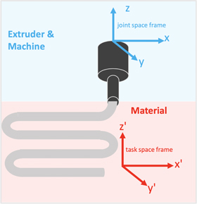
Figure 1. The two coordinate frames in AM are the joint space frame, defining the machine and extruder motion, and the task space frame, which represents the material spatial placement. Due to imperfect coordination between the two motion frames, there is no guarantee that perfect motion in the joint space results in the as-designed task space results.
Download figure:
Standard image High-resolution imageFor much of the prior work in precision AM, the machine control has been the focus and precision control in the joint space has been assumed to be equivalent to precision control in the task space. Previous work used encoder signals of each machine axis for process feedback [8, 25], which only gives information on the machine itself. Due to imperfect coordination between the joint and task spaces, however, there is no guarantee that perfect regulation of the joint space results in the as-designed task space results. The loss of coordination arises from nozzle alignment errors, nozzle tip displacement errors due to mechanical forces, and the highly nonlinear material behavior. The errors accumulate due to a lack of direct process monitoring in the task space. Using sensing and control to monitor and improve the actual material placement has received less attention. In fact, there are currently no 3D printers on the market with closed loop process control monitoring the material placement.
One method to improve material placement is to develop a detailed material model to try to predict the material behavior during fabrication. Models, however, are subject to uncertainty in materials and processing conditions. The difficulty in obtaining an accurate model is particularly true for manufacturing processes that combine complex material processing behavior with mechanical or electro-mechanical machine behavior [26, 27]. Modeling and control of extrusion dynamics in DW printing is difficult due to the nonlinear behavior of yield-pseudoplastic fluids. In [28], the output volumetric flow rate for a DW printing system was carefully determined using machine vision and compared to nonlinear and linearized models, as shown in figure 2. The nominal behavior in figure 2 is captured by the multiple models shown in red as solid and dashed lines. However, the experimental data (dark trace) in figure 2 illustrate deviation from the model and a widespread in the data (shaded area). These data demonstrate the significant modeling error inherent in these types of systems. Therefore, relying on a material model may result in a final part with significant dimensional errors since the model cannot precisely predict the material behavior during extrusion.
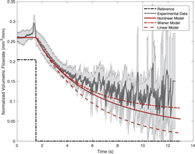
Figure 2. Comparison of volumetric flow rates of the material obtained from model simulations to flow rates measured on the experimental system of [28]. The light gray shaded regions correspond to one standard deviation. Image reproduced with permission from [28].
Download figure:
Standard image High-resolution imageAlternatively, adding a sensor to monitor material placement during biofabrication can improve part fidelity. While in situ process monitoring is well established in conventional machining [29], in situ process monitoring for AM remains sparse [30]. Further, much of the work for in situ process control in AM is in metal manufacturing using AM techniques not commonly used in the biofabrication field like laser powder bed fusion [31] using sensors such as x-ray imaging and diffraction [32] and optical microscopy [33]. To transition 3D bioprinting into a clinically relevant biofabrication platform, 3D metrology tools must be developed to assess and correct for material placement error [2, 12], [34, 35].
There is some effort in assessing and quantifying geometric defects in the 3D bioprinting literature [2, 34, 35]. In [2], the accuracy of the bioprinting process was evaluated for simple rectilinear lattice structures using calipers post fabrication. The channel dimensions of the printed part were compared to the dimensions of the design model to compute the printing accuracy, which was defined as the percent overlap of printed to designed area. In [35], the geometry of 3D printed bone scaffolds was evaluated using x-ray tomography post print. The width of internal pores was determined from 2D cross-sections and compared to the as-designed pore shapes. In [34], the geometric accuracy of 3D printed aortic valve conduits was quantified post print using Micro-CT. The scans were reconstructed into stereolithography (STL) geometries and compared to the nominal model to evaluate external geometric fidelity. Further, the internal geometric fidelity was assessed by comparing the scans and nominal model slice-by-slice in the X–Y plane. While there is clear effort in identifying material placement error, the assessments are performed post process and the sensing tools utilized are completely separated from the printing platform. Moreover, there is currently no solution to improve shape fidelity using these error measurements.
We propose that the solution to improve the accuracy of 3D bioprinting is twofold. First, the development of an accurate sensing method that is incorporated into the printing process is required to enable in situ process control. Second, the information from this sensor must be used intelligently to determine how to adjust axes reference trajectories to improve fabrication. In this work, we develop a novel sensing and control strategy to enable process monitoring and correction in the material deposition frame. We focus on monitoring and correcting spatial material placement for a single layer, and use a non-contact, in situ process monitoring sensor that is integrated into the AM system to measure the spatial material placement. An automated image processing algorithm uses the sensor output to calculate the material placement error, which is then used to modify the machine reference trajectory to achieve the as-designed material placement. To validate the approach, the process monitoring system is implemented on an experimental platform to demonstrate material fabrication improvement. Since there is currently no standard method to quantify part fidelity, we propose using specific error calculations to quantitatively assess the performance improvement. The technique is applied to three types of printing paths commonly used in the bioprinting literature to illustrate how the approach is generalizable to a wide range of extrusion-based bioprinting applications.
2. Methods
2.1. System
We apply our generalized process control method to a pneumatic-based micro extrusion system shown in figure 3. A pressure regulator with output pressure ranging from 0 to 30 psi is used to apply constant pressure to a reservoir of ink, which in turn extrudes ink through a nozzle in the form of cylindrical rods. We use a calcium phosphate-based ceramic material system for applications in bone repair and regeneration [7, 36]. For the current work, we use a general-purpose stainless-steel nozzle tip with a 0.41 mm internal diameter of 0.41 mm and a 6.35 mm tip length. However, the nozzle dimensions could be varied based on commercially available tips. The ink is extruded on a substrate that was spray-painted black to ensure contrast between the ink and the substrate for better image processing. The nozzle tip is positioned approximately 0.3 mm above the substrate, and an applied pressure of 20 psi is used for extrusion.
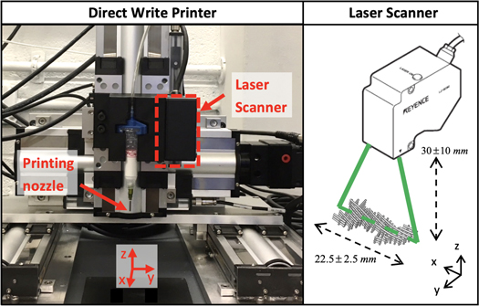
Figure 3. Left: direct Write printer with standard Cartesian coordinates. The system uses pneumatic extrusion, and a laser scanner is fixed to the extruder head to enable direct process feedback. Right: The process sensor is a Keyence LJ-G030 laser scanner, which uses the principle of triangulation to determine the height of the target object.
Download figure:
Standard image High-resolution imageA non-contact 2D laser displacement scanner (Keyence LJ-G030) is mounted to the extruder head on the Z axis to enable direct process control. The scanner uses the principle of triangulation to reproduce the surface profile. When the laser emitted from the scanner hits the target, the reflected light is mapped onto a light-receiving element to determine the object distance from the scanner. The scanner output is an analog signal equal to the target height. The laser scanner has a measuring range of 30 ± 10 mm in the Z direction, and a 22.5 ± 2.5 mm width along the laser profile in the X direction (figure 3, right). The repeatability is 1 and 5 μm for Z-height measurements and X axis width measurements, respectively. The axes move the scanner across the part along the Y direction, so the Y axis spatial resolution depends on the speed of the axes. The weight of the scanner is 0.64 lbs, so it is easily mounted on the end effector. A dSPACE MicroLab Box and the Control Desk software is used to control the machine and pneumatic extruder. A custom MATLAB algorithm processes the scanner data and performs several image processing steps, which are reviewed in section 2.3. Python is used to communicate between MATLAB and Control Desk to implement the process control approach.
2.2. Range of reference trajectories in extrusion-based bioprinting
To demonstrate our process monitoring technique, we apply the approach to three types of reference trajectories commonly used in the bioprinting literature. After a thorough literature assessment, we have grouped the extrusion-based biofabrication techniques into three categories based on the type of motion profile used for fabrication (figure 4). The categories are on a spectrum. On one end is the Rectilinear with Turnarounds classification, shown in the top box in figure 4, which uses rectilinear patterns with turnarounds to trace out curved boundaries. This type of fabrication pattern is common when standard G-code is used as a motion path for the 3D printer. Typically, the machine software slices the as-designed CAD file into layers with a specific infill path, which is a repetitive structure used to take up space inside a given shape within a single layer. The examples in figure 4 include a human-scale ear [37] and an aortic valve [34] that each use rectilinear lines to trace out internal and external curved features.
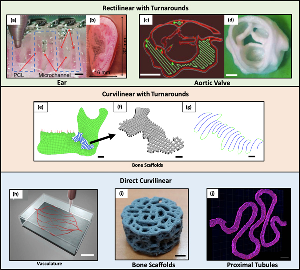
Figure 4. The three categories of extrusion-based bioprinting trajectories: rectilinear with turnarounds, curvilinear with turnarounds, and direct curvilinear. (a) Image of a 3D printing process organ fabrication, which uses a rectilinear pattern to fabricate a layer of an ear construct (adapted from [37]). Scale bar is 0.5 mm. (b) Photograph of the final 3D printed ear cartilage construct [37]. (c) A single layer of the STL file for an aortic valve construct [34]. The printing software sliced the geometries into layers and generated extrusion paths for each layer (red: contour, green: fill-in-paths). Scale bar is 10 mm. (d) The final printed valve construct [34]. Scale bar is 10 mm. (e) Finite element model of a mandible with a defect filled with the optimal design for a bone scaffold (adapted from [38]). Scale bar is 5 mm. (f) CAD model for two alternating layers of the curvilinear bone scaffold design [38]. Scale bar is 2 mm. (g) Reference trajectory pattern for one of the layers from (f), where curved turnarounds (green lines) were added to ensure smooth flow between curvilinear rods. Scale bar is 3 mm. (h) Schematic of the fabrication of a fugitive ink into a physical gel reservoir for printing of microvascular networks from [5]. Scale bar is 10 mm. (i) Image of a printed porous bone scaffold with continuous curvilinear rods (adapted from [35]). Scale bar is 1 mm. (j) A 3D rendering of a printed convoluted proximal tubule acquired by confocal microscopy (adapted from [39]). Scale bar is 1 mm.
Download figure:
Standard image High-resolution imageOn the other end of the spectrum is the Direct Curvilinear classification, shown as the bottom box in figure 4. For this classification, the curvilinear patterns are fabricated directly. The curvilinear structure is user-defined and the ink is extruded directly along the curved paths. The examples in figure 4 include the fabrication of microvasculature [5], bone scaffolds with continuous curvilinear lines [35], and proximal tubules [39].
The third classification, Curvilinear with Turnarounds, lies in the middle of the spectrum (middle box, figure 4). This category has features from both sides of the spectrum. Similar to the Rectilinear with Turnarounds group, turn arounds (illustrated as green lines in figure 4(g)) are used to ensure manufacturability and to change axis directions. The rods in between turnarounds (illustrated as blue lines in figure 4(g)), however, are curvilinear, similar to the Direct Curvilinear group. Fabrication of the pattern shown in figure 4(g) is a continuous process and the two colors are used to highlight the turn around and rod regions. This type of fabrication pattern is common for scaffold fabrication, specifically lattice structures with curved rods. The example application in this classification is patient-specific bone scaffolds with spatially-varying architecture for complete bone regeneration (figures 4(e)–(g)) [38]. The non-periodic scaffold is designed using topology optimization techniques to obtain maximal stiffness for a prescribed porosity in order to promote osteointegration [38].
We use an example fabrication pattern from each group to demonstrate the steps and effectiveness of the process monitoring technique presented in this paper. Specifically, we use the aortic valve reference trajectory (figure 4(c)) to represent the Rectilinear with Turnarounds group, the bone scaffold reference trajectory (figure 4(g)) for the Curvilinear with Turnarounds group, and the proximal tubule reference trajectory (figure 4(j)) for the Direct Curvilinear Group.
2.3. Process monitoring steps
Our process monitoring technique uses direct process feedback in the task space frame to monitor spatial material placement. The main goal of our technique is to use the laser scanner data to redefine the reference trajectory in the joint space frame to achieve the as-designed material placement in the task space frame. The technique is a five-step, automated process (figure 5) that compensates for the error pattern by adjusting the path the machine axes follow in the joint space frame
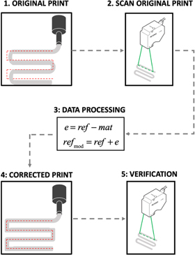
Figure 5. The proposed five-step process sensing method to improve spatial material placement.
Download figure:
Standard image High-resolution imageWe first define the task space error as the difference between the as-designed reference trajectory and the material centerline estimate. The first step is to fabricate the Original Print, which is defined as material extrusion along the original reference trajectory. The extruded part in this step will not be used in application and is instead solely used to define the task space error. As illustrated in figure 5, the spatial material placement is expected to differ from the as-designed reference trajectory (red dashed line).
In the second step the motion system moves the laser scanner across the Original Print after the entire pattern is fabricated. The laser scanner outputs a vector of height measurements of the fabricated part at sample points along the laser profile in the X direction at a set sampling rate. We combine the collection of height measurements at each sampling time and store the 3D point cloud as a matrix. The motion system must move at a constant speed during scanning since the rows and columns of the matrix correspond to a cartesian grid with equal spacing and since the laser scanner outputs data at a set sampling rate
The third step uses a custom image processing algorithm to determine the task space error and modified reference trajectory for the joint space frame. We include the details in section 2.3 to briefly review the main steps of the image processing algorithm.
In Step 4, the DW printer fabricates the Corrected Print using the modified reference trajectory from Step 3. As shown in figure 5, since the algorithm compensates for the error from the Original Print, the material centerline estimate is more aligned with the as-designed reference trajectory, still the red dashed lines. Finally, the laser scanner is again used in Step 5 to verify material placement improvement. The axes move the laser scanner across the part fabricated in the Corrected Print to demonstrate that the printed layer exhibits geometric fidelity. Similar to Step 2, the image processing algorithm, discussed in section 2.3 calculates the new task space error of the Corrected Iteration.
The process sensing method can be implemented multiple times to further improve the error metrics. For a second iteration of Correction, the five steps outlined in figure 5 are repeated. Here the 'Corrected Print' is now the 'Original Print'. The modified reference trajectory computed from the first iteration Corrected Print is used as the reference trajectory for the second iteration Corrected Print.
2.4. Custom image processing algorithm
The custom image processing algorithm includes eight main steps, illustrated in figure 6, to determine the material error ( ). The required inputs for the image processing algorithm include the 3D point cloud (
 ), the spatial vectors along the laser profile (
 ) and along the scanning direction (
 ), the Z-height minimum (
 ) and maximum (
 ) threshold values to filter out the noise and isolate the extruded material in the scanner data, and the original reference trajectory (
 ). We use the bone scaffold pattern from [38] as the example reference trajectory to illustrate the steps of the image processing algorithm.
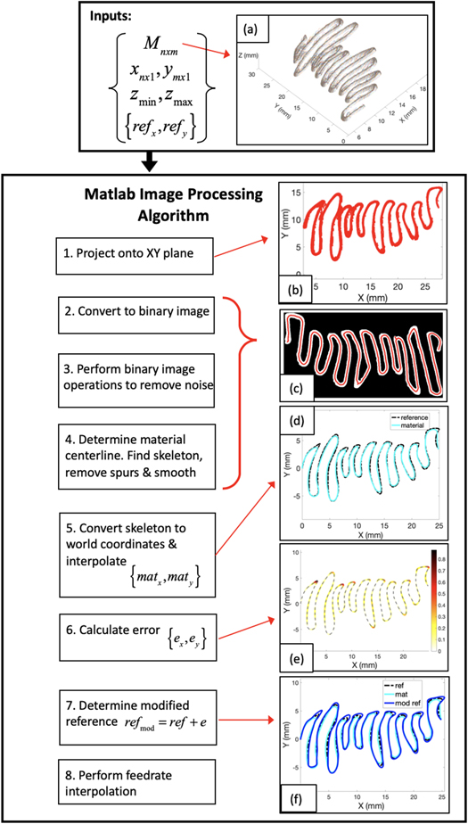
Figure 6. Diagram illustrating the required inputs and steps of the image processing algorithm. The inputs include the 3D point cloud output of the laser scanner  the spatial x and y vectors representing the coordinates along the laser profile (
 ) and along the scanning direction (
 ), the Z-height minimum and maximum threshold values (
 ) for projection onto the XY plane, and the original reference trajectory (
 ).
).
Download figure:
Standard image High-resolution imageThe first step of the image processing algorithm is to project the 3D point cloud data onto the XY plane. A for loop walks through each entry of the point cloud to determine if the Z-height at a given Cartesian location is in the  range. The X- and Y-locations of each Z-height in this range are stored in a 2D matrix. The second step is to convert the resulting 2D matrix to a binary image. The third step requires several built-in MATLAB image processing functions to remove noise and isolate the extruded material pattern in the binary image.
After filtering the binary image, the fourth step is to extract the material path, which is defined as the material centerline estimate. This is accomplished through skeletonization, an image processing technique that reduces all objects in a 2D binary image to a one-pixel width line that preserves the essential structure of the image. The skeleton of the bone scaffold path is shown as a red line in figure 6(c). The filters in this step remove spurious lines and ensure a smooth material centerline estimate.
In Step 5, the algorithm converts the skeleton data points defined for the binary image back to Cartesian coordinates stored in a two-column vector. These coordinates are interpolated so that the vector has the same size as the reference trajectory vector. Upon completion of this step, the material centerline estimate is in an appropriate form to compare it to the reference trajectory and define the task space error, figure 6(d).
In the sixth step, we define the task space error using the normal vector approach (figure 7) [40]. Due to previously mentioned errors in the fabrication process, the spatial material path (blue dashed line) deviates from the as-designed reference trajectory (black dotted line). The algorithm steps through each point in the reference trajectory vector and identifies the error vector at each point on the material path that intersects with the normal line from the reference trajectory. Figure 6(e) shows the magnitude of the error vector at each point along the reference trajectory for the bone scaffold trajectory.

Figure 7. Example path representing the normal vector approach.
Download figure:
Standard image High-resolution imageIn Step 7, the error vector is used to modify the nominal reference trajectory using the mirror approach [40]. First, the algorithm determines the compensation vector by taking the mirror image of the error vector with respect to the reference trajectory (figure 7). The modified reference trajectory (red solid line) is the locus of points at the heads of all compensation vectors for all points on the nominal reference trajectory. The modified reference trajectory is the modified machine axes path in the joint space frame to produce an actual material path that coincides with the as-designed trajectory. Figure 5(f) compares the modified reference trajectory for the bone scaffold pattern to the nominal reference trajectory.
The control points contained in the modified reference trajectory vector from Step 7 are not necessarily equally spaced, resulting in a non-constant speed along the curve. In CNC machining, the tool speed along a curve is termed the feedrate. There are a number of real-time interpolation algorithms designed to move CNC machines at a constant feedrate to ensure a smooth cut or surface finish [41–43]. In AM, it is equally as important to move the axes and extruder head along a curve at a constant rate to ensure smooth material flow and therefore uniform ink width along the path. A non-constant axis speed would result in uneven material widths along the curve; higher rates would lead to thinner ink width while slower rates would lead to thicker ink widths.
In Step 8, the algorithm converts the modified reference trajectory to the required format with a constant feedrate for real-time implementation on the machine axes. The algorithm interpolates the modified reference trajectory to ensure a constant speed along the curve using an algorithm titled 'interparc' from the MATLAB File Exchange that is readily available to the public [44]. Essentially, 'interparc' generates a new set of points that are uniformly spaced along the same curve. Figure 8 shows the speed along the modified reference trajectory for the bone scaffold pattern before (blue solid line) and after (red dashed line) feedrate interpolation. After interpolation, the axes and extruder head move along the curve at a constant rate, here 3 mm s−1.
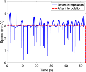
Figure 8. Speed along the bone scaffold reference trajectory curve before and after interpolation. After interpolation, the speed remains at 3 mm s−1 along the entire curve.
Download figure:
Standard image High-resolution image3. Results
3.1. Original prints
For the Original Print of all three reference trajectories, the material path in the task space frame differs from the as-designed reference trajectory and the axes motion in the joint space frame, motivating the need for direct process control. The data plotted in figure 9 compare the material centerline estimate (red line), axes motion (blue line), and reference trajectory (black dashed line) for the Original Print. These three vectors are plotted on top of the laser scanner data projected onto the XY plane (cyan blue region). The material and axes data are from the Original Print before the process control method is applied. The material centerline fit (red line) is the estimate of the material path of the actual print, which differs from the desired material path (black dashed line). Further, the material centerline fit may not always track the axes path (blue line), illustrating the discrepancy between the task and joint space frames.
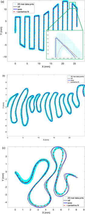
Figure 9. The 2D material data points (cyan blue shaded region), material centerline fit (red dashed line), machine axes path (blue solid line), and reference trajectory (black dotted line) for each reference pattern. The black dotted line is the desired print and the red dashed line is the actual print. (a) Aortic reference trajectory, (b) scaffold reference trajectory, and (c) tubule reference trajectory. The data plotted in figure 9 are the output of the image processing algorithm for the Original Print.
Download figure:
Standard image High-resolution image3.2. Corrected prints
After the process sensing control method is applied, there is noticeable improvement in spatial material placement for all three reference trajectories. Figure 10 shows an image overlay for each pattern to compare images of extruded material between the Original and Corrected Prints. The images were captured directly above the fabricated pattern on top of the black substrate and show a top down view of the XY plane in the task space frame. The white material is the fabrication pattern of the Original Print where the nominal reference trajectory was used in the joint space frame. The shaded material with reduced transparency is the fabrication pattern of the Corrected Print after application of the process monitoring technique where the modified reference trajectory was used in the joint space frame. The as-designed reference trajectory is shown as a black dashed line. For all three reference trajectories, the blue material path (Corrected Print) more closely tracks the as-designed reference trajectory relative to the white material path (Original Print).
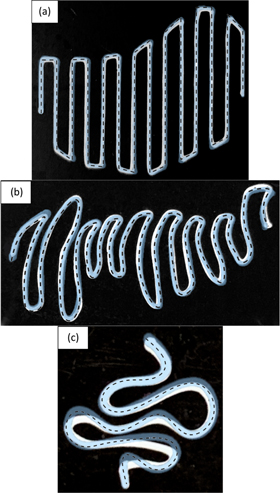
Figure 10. Image overlay for each fabrication pattern. The white material is the fabrication pattern of the Original Print and the light blue with reduced transparency is the fabrication pattern of the Corrected Print. The as-designed reference trajectory for each pattern is shown as a black dashed line. (a) Aortic reference trajectory, (b) scaffold reference trajectory, and (c) tubule reference trajectory.
Download figure:
Standard image High-resolution imageThe task space error is reduced along each of the reference trajectories. Figure 11 shows the magnitude of the task space error plotted spatially for each example reference path with the as-designed reference trajectory as a black dashed line. The color shading of the trajectory shows the error magnitude at each point on the reference trajectory. The scale bar for the color shading is on the right-hand side, where a darker red color indicates a larger error. The XY plots on the left and right side represent the task space errors from the Original and Corrected Prints, respectively. For all three reference trajectories, the color shading for the Corrected Print contains noticeably less dark red regions.
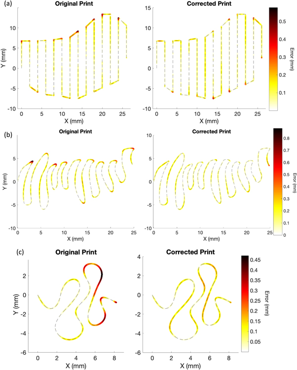
Figure 11. The task space error magnitude at each point on the reference trajectory represented as color shading of the trajectory. The scale bar for the color shading of each reference is on the right side, with a darker color representing a larger error magnitude. The XY plots on the left and right show the task space error for the Original and Corrected Prints, respectively. (a) Aortic reference trajectory, (b) scaffold reference trajectory, and (c) tubule reference trajectory.
Download figure:
Standard image High-resolution imageModifying the axes reference trajectory in the joint space frame resulted in a material path that was more aligned with the as-designed reference trajectory. The images in figure 12 illustrate two additional outputs of the custom image processing algorithm for each reference pattern: the modified reference trajectories and the material centerline estimates. The images on the left-hand side compare the nominal axes reference trajectory, 'Ref Orig' that is used to fabricate the Original Print, with the modified axes reference trajectory, 'Ref Corr' used to fabricate the Corrected Print. The images on the right-hand side compare the material paths resulting from the two different reference trajectories. The as-designed reference trajectory is shown as a black dotted line, the material centerline for the Original Print is shown as a red dashed line, and the material centerline estimate for the Corrected Print is shown as a green solid line. The images on the right-hand side of figure 12 illustrate that the material path for the Corrected Print is shifted closer to the as-designed reference trajectory by using the corresponding modified axes reference trajectory on the left-hand side.

Figure 12. Left: comparison of the nominal reference trajectory (black dotted line, Ref Orig) used to fabricate the Original Print with the modified reference trajectory (green solid line, Ref Corr) used to fabricate the Corrected Print. Right: comparison of the material path from the Original Print (red dashed line, Mat Orig) to the material path from the Corrected Print (green solid line, Mat Corr). The black dotted line shows the as-designed reference trajectory. (a) Aortic reference trajectory, (b) scaffold reference trajectory, and (c) tubule reference trajectory.
Download figure:
Standard image High-resolution imageTable 1 lists the quantitative error metrics for each example reference pattern. The first metric is the two-norm of the task space error, which corresponds to the root mean square (rms) error. The second metric is the infinity-norm of the task space error, which is the maximum absolute value of the entries of a vector. For the aortic valve reference, there is an 11% decrease in the two-norm and a 19% decrease in the infinity-norm. For the bone scaffold pattern, there is a 32% decrease in the two-norm and a 49% in the infinity-norm. For the tubule pattern, there is a 33% decrease in the two-norm and a 62% decrease in the infinity-norm.
Table 1. Quantitative error metrics comparing the Original and Corrected Prints.
| Error metric | ||||||
|---|---|---|---|---|---|---|
| Two-norm | Infinity-norm | |||||
| Reference | Original print | Corrected print | Percent reduction | Original print | Corrected print | Percent reduction |
| Aortic | 26.5 | 23.4 | 11% | 0.6 | 0.5 | 19% |
| Scaffold | 35.5 | 24.2 | 32% | 0.9 | 0.5 | 49% |
| Tubule | 17.7 | 11.9 | 33% | 0.5 | 0.2 | 62% |
3.3. Additional iterations
The data presented in section 3.2 are for one iteration of Correction. An additional Correction iteration was performed for the tubule reference trajectory to further reduce the material placement error. Modifying the axes reference trajectory for a second iteration in the joint space frame resulted in a material path that was more aligned with the as-designed reference trajectory and a reduction in the task space error.
The data in figure 13 compare the modified reference trajectories and the material centerline estimates from the custom image processing algorithm of the Original Print and the two iterations of the Corrected Print. The images on the left-hand side compare the nominal axes reference trajectory, 'Ref Orig' that is used to fabricate the Original Print, with the modified axes reference trajectories, 'Mod Ref It 1' and 'Mod Ref It 2', used to fabricate the first and second iterations of the Corrected Print, respectively. The images on the right-hand side compare the material paths resulting from the three different reference trajectories. The as-designed reference trajectory is shown as a black dotted line, the material centerline for the Original Print is shown as a blue double dashed line, and the material centerline estimates for the first and second Corrected Prints are shown as a green solid line and red dashed line, respectively. The image on the right-hand side of figure 13 illustrates that the material path for the second iteration of the Corrected Print is shifted closer to the as-designed reference trajectory by using the corresponding modified axes reference trajectory on the left-hand side.
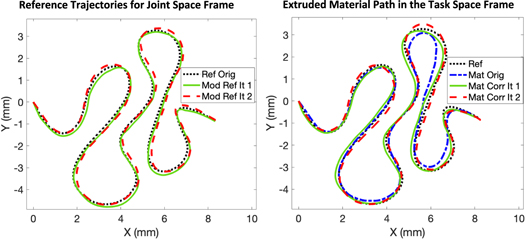
Figure 13. Left: comparison of the nominal reference trajectory (black dotted line, Ref Orig) used to fabricate the Original Print with the modified reference trajectories used to fabricate the first (green solid line, Mod Ref It 1) and second iterations (red dashed line, Mod Ref It 2) of the Corrected Prints. Right: comparison of the material path from the Original Print (blue double dashed line, Mat Orig) to the material path from the first iteration of the Corrected Print (green solid line, Mat Corr It 1) and the material path from the second iteration of the Corrected Print (red dashed line, Mat Corr It 2). The black dashed line shows the as-designed reference trajectory.
Download figure:
Standard image High-resolution imageThe error improvement is further shown in figure 14, which shows the magnitude of the task space error plotted spatially for the Original Print, the first iteration of Correction (Corrected Print It 1), and the second iteration of Correction (Corrected Print It 2). The as-designed reference trajectory is indicated as a black dashed line. The color shading of Corrected Print It 2 contains noticeably fewer yellow regions. However, the location of the larger errors, indicated by a darker red color, shifted along the reference trajectory.
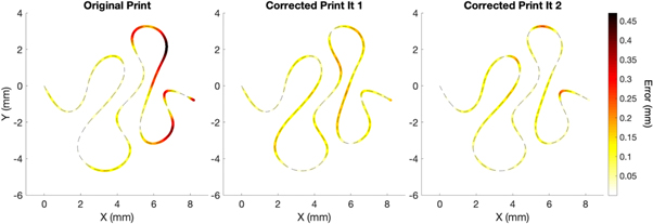
Figure 14. The task space error magnitude at each point on the reference trajectory represented as color shading of the trajectory. The scale bar for the color shading of each reference is on the right side, with a darker color representing a larger error magnitude. From left to right, the XY plots show the task space error for the Original Print, the Corrected Print from the first iteration of correction, and the Corrected Print from the second iteration of correction.
Download figure:
Standard image High-resolution imageTable 2 compares the quantitative error metrics for each of the Correction iterations. There was a 24% reduction in the error two-norm between the two correction iterations, with no change in the error infinity-norm. The results indicate that the additional correction iteration resulted in less overall error, but the max error value was not further reduced.
Table 2. Quantitative error metrics comparing iterations 1 and 2 of the Corrected Prints for the tubule reference trajectory.
| Error metric | |||||
|---|---|---|---|---|---|
| Two-norm | Infinity-norm | ||||
| Corrected print It 1 | Corrected print It 2 | Percent reduction | Corrected print It 1 | Corrected print It 2 | Percent reduction |
| 11.9 | 9.1 | 24% | 0.2 | 0.2 | 0% |
3.4. Repeatability
To evaluate the repeatability of the proposed process control method and manufacturing system, we fabricated two identical runs of a rectilinear, raster reference trajectory. We compared the material centerline estimates, calculated modified reference trajectories, and error calculations. Steps 1–3 in figure 5 were performed for each fabricated scaffold, and the Original Print of each scaffold (Scaffold A and B) is shown in figure 15. The data presented in figure 16 below compare the material centerline estimates and suggested modified reference trajectories. The image on the left-hand side compares the material centerline estimate of the two scaffolds. The image on the right-hand side compares the nominal axes reference trajectory, 'Ref Orig' that was used to fabricate the two Original Prints, with the calculated modified axes reference trajectories. The magnitude of the task space error for each scaffold is plotted in figure 17 with the as-designed reference trajectory shown as a black dashed line. The color shading of the trajectory shows the error magnitude at each point on the reference trajectory. The two XY plots on the left side represent the task space errors from Scaffolds A and B, respectively. The XY plot on the right side represents the error differential between the two scaffolds, which has a different scale bar.
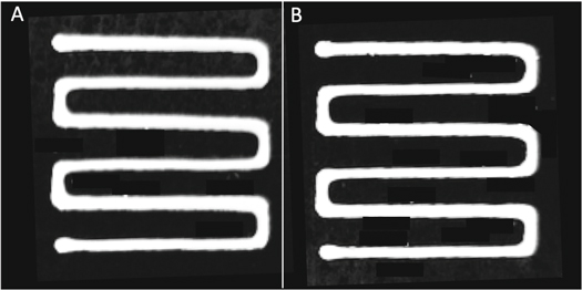
Figure 15. The Original Prints of the two repeated rectilinear scaffold reference patterns. (Left) Scaffold A. (Right). Scaffold B.
Download figure:
Standard image High-resolution image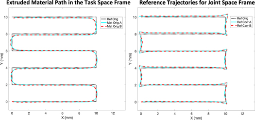
Figure 16. Left: comparison of the material centerline estimates from the two Scaffold Original Prints. The material centerline estimate for Scaffold A is shown as a cyan blue solid line, and the material centerline estimate for Scaffold B is shown as a red dashed line. The black dotted line shows the as-designed rectilinear scaffold reference trajectory. Right: comparison of the modified reference trajectories calculated for Scaffolds A (cyan blue solid line) and B (red dashed line). The nominal reference trajectory is again shown as a black dotted line.
Download figure:
Standard image High-resolution image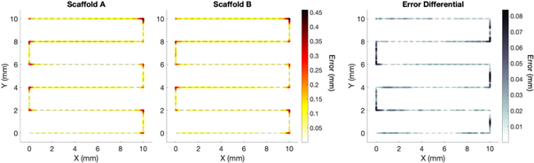
Figure 17. Left: the task space error magnitude at each point on the reference trajectory represented as color shading of the trajectory. The scale bar for the color shading of each reference is on the right side of the image for Scaffold B, with a darker color representing a larger error magnitude. The XY plots on the left and right show the task space error for Scaffold A and Scaffold B, respectively. Right: The task space error differential at each point on the reference trajectory represented as color shading of the trajectory. Note the different scale bar on the right-hand side.
Download figure:
Standard image High-resolution image
We evaluated the process repeatability relative to part feature size. The raster trajectory has feature sizes of 10 mm along the X direction and 2 mm along the Y direction. The largest error between the two scaffolds is 0.08 mm, which is less than 4% of the 2 mm feature size and less than 1% of the 10 mm feature size. Further, table 3 lists the quantitative error metrics for each scaffold. There is a 0.37% difference in the error two-norm and a 4.4% difference in the error infinity-norm. Since the calculated errors and modified reference trajectories were similar, measurement system and fabrication process are repeatable within 5% which is sufficient for many biofabrication applications.
Table 3. Quantitative error metrics comparing the original prints for Scaffolds A and B.
| Error metric | |||
|---|---|---|---|
| Two-norm | Infinity-norm | ||
| Scaffold A | Scaffold B | Scaffold A | Scaffold B |
| 16.08 | 16.14 | 0.44 | 0.46 |
4. Discussion
The process control approach in this work differs significantly from other AM systems that focus on motion control of the machine in the joint space frame of reference. Our five-step process monitoring technique uses direct process feedback in the task space frame to determine the spatial material placement error. We compensate for the error iteration by iteration by redefining the joint space reference trajectory to reduce the material placement error in the task space frame in the next iteration. The entire process control method takes less than 5 min for implementation.
The field of bioprinting not only lacks an established process to measure the error, but also a standard error metric to quantify the fidelity of printed constructs. In this work we used the error two-norm and the error infinity-norm since these are commonly used performance metrics in the field of manufacturing systems to assess performance improvement. There were clear quantitative improvements for all three reference patterns in the two important error metrics used to assess improvement in spatial material placement improvement. A reduction in the error two-norm implies there is less overall spatial material placement error throughout each of the patterns. Minimizing the error two-norm is especially important to ensure structural stability and to ensure the part can fit inside the as-designed in vivo location. For example, the as-designed bone scaffold must have precise dimensions in order to fit and anchor inside the defect site.
Moreover, reducing the infinity-norm minimizes the worst-case error, implying there was fabrication improvement in hard to print regions, such as tight corners or areas with high curvature. This is important for research studies in which the investigators are testing a certain geometric variable of printed constructs, such as the effect of rod curvature on the amount of bone growth inside a bone scaffold. It is important for the fabricated parts to closely follow the design since manufacturing defects in the bioprinted constructs can limit their in vivo functionality and skew the study results. For example, the amount of bone regeneration in bone scaffolds fabricated by AM is hindered by the presence of manufacturing defects [45] since the material overbuild physically blocks bone growth inside the scaffold.
The results in figure 9 demonstrate that relatively accurate reference tracking in the joint space frame does not imply accurate material placement in the joint space frame. For all three example patterns, the axes (blue line) closely followed the as-designed path, and the material and axes paths do not coincide. The results further validate the need for process control in AM since joint space motion cannot precisely predict material behavior in the task space frame.
The process control method in this work was most effective in improving material placement for the tubule and bone scaffold patterns. The percent reduction in the error two-norm for the tubule and bone scaffold patterns was roughly 2.8 times larger than the percent reduction for the aortic pattern. Moreover, the percent reduction in the error infinity-norm was 3.25 times larger for the tubule pattern and 2.57 times larger for the bone scaffold pattern relative to the aortic pattern. The tubule pattern was representative of the Direct Curvilinear group and the bone scaffold pattern was representative of the Curvilinear with Turnarounds group. Both of these groups consist of curved features along the entire trajectory. The results imply that the current process control method is more effective for fabrication improvement of curvilinear patterns more so than patterns with mostly straight trajectories combined with sharp corners at the turnarounds, like the Rectilinear with Turnarounds group.
As illustrated in section 2.3, additional iterations of the process control method can further improve the spatial resolution of the fabricated construct. There are several process parameters that ultimately limit the achievable spatial resolution and the ability to achieve the desired manufacturing tolerances for a given application. One process parameter is the resolution of the sensing element which will limit the amount of error that can be detected. In addition, fine motion behavior of the actuation elements used to move each of the axes during fabrication is required to accurately print tight corners or small radii of curvature. Further, the resolution of the material system, which includes the rheologic properties of the material, the extrusion method and the nozzle size, will affect the final spatial resolution and repeatability of the process.
While the 2D laser displacement scanner was effective at imaging the extruded material, there is an opportunity to improve the material centerline estimate from the 2D data. The material centerline estimate of the 2D laser scanner data was obtained through an image processing method termed skeletonization. The skeletonization process works better for curvilinear paths relative to sharp turnarounds, which may explain why our process sensing method was more effective for the Direct Curvilinear and the Curvilinear with Turnarounds groups relative to the Rectilinear with Turnarounds group. The skeletonization process does not accurately estimate the material centerline at sharp turnarounds with material overbuild, as shown in the insert of figure 9 for the aortic Rectilinear with Turnarounds path. A more accurate material centerline estimate would be shifted up and to the left in the figure 9 insert.
Moreover, to extend this process monitoring approach to applications that use DW printing for solid fill of internal spaces, an alternative strategy can be used to identify the material centerline estimate. Instead of using the skeletonization approach which analyzes the data in the XY plane, the layer topology can be obtained from the YZ plane of the laser scanner data. The rod centerline estimate can be obtained using the output rod peaks and valleys in the YZ plane. Future versions of the image processing algorithm provide an opportunity to improve laser scanner data processing to more accurately estimate the material path and ultimately improve error correction. The second iteration of Correction presented in section 3.3 further reduced the error two-norm but did not improve the infinity-norm. More accurate material centerline estimates could further improve the effectiveness of the approach and ultimately reduce the final converged error after multiple iterations of the process. The development of improved process control methods should work at the intersection of AM and computer science in order to leverage the advancements in image processing to improve material fabrication.
Currently, our process control method improves the spatial material placement for a single layer part with curvilinear patterns. The approach, however, can be extended to multi-layer parts. A simple example for multi-layer extension is a woodpile pattern of two repeating patterns, such as the rectilinear raster trajectory in figure 16 which would be rotated by 90° for each successive layer. The final multi-layer construct can likely be improved by adjusting the joint space frame reference trajectories for each layer. The five-step process sensing method would be performed for each layer pattern offline to determine the modified reference trajectories. The modified reference trajectories would be combined and implemented in real-time to fabricate the full multi-layer scaffold. There are numerous difficulties associated with extension to more difficult multi-layer parts, which are outside the scope of this investigation.
The task space error defined in this work was defined as the error between the material centerline and reference trajectory. In future work we will extend the error calculation to multiple dimensions to monitor material flow rate. A second error dimension would consider the material width along the curve to ensure consistent material flow to eliminate regions of material overbuild or underbuild. Furthermore, a third error dimension would consider the height and degree of flatness of each layer. Adding process control to this third error dimension would be used to ensure flat layers and improve the stability and integrity of multi-layer parts. The laser scanner used for the single dimension error in this work would also work for the two additional error metrics. Implementing additional control dimensions will further enhance our process control method and improve the geometric fidelity of 3D constructs.
In addition to the trial-to-trial correction process outlined in this work, the laser scanner data could be used direct feedback within each iteration to respond to deviations from the intended print trajectory and iteration varying disturbances. The coupling of this in situ process monitoring data and the iteration-to-iteration correction could be coupled to further enhance the spatial material placement. This coupling and real-time process control, however, requires additional data processing and implementation complexity outside the scope of the current work.
While we applied the process monitoring technique to a specific DW printing platform with a calcium phosphate material system, the generalized approach can be extended to other extrusion-based platforms and other AM techniques, such as fused deposition modeling (FDM), to improve the spatial material placement in other bioprinting applications. The results presented in section 3.4 indicate the fabrication process in this work is repeatable. For systems with random variance, the method can be adapted to include statistical approaches to determine the average material behavior. Statistical methods are commonly used in the literature to characterize ink behavior during fabrication. Baturynska et al collect data from two identical runs to evaluate the dimensional accuracy of parts fabricated by FDM [46]. The final value of each dimensional feature is calculated as a mean of repeated measurements [46]. This approach can be extended to the method presented in this work. The average of a few trials of the 'Original Print' would be used to obtain an estimate of the material error. The calculation of the modified reference trajectory would use the average material error for correction at the next iteration.
5. Conclusion
In this work we develop a novel sensing and control method to enable process monitoring and improve precision of spatial material placement in 3D bioprinting. Moreover, we propose using the error two-norm and error infinity-norm as a means to quantify the part fidelity, which is an additional important contribution to the field of bioprinting. For process monitoring, we use a non-contact, laser displacement scanner that is integrated into the AM system. Our technique modifies the machine path that results in the as-designed material placement and does not require extensive training or system information. After initial fabrication of the as-designed pattern, the axes move the laser scanner across the part for inspection, and the error pattern is determined with a custom image processing algorithm. The error is compensated by defining a modified reference trajectory containing the set of points that deviate from the as-designed reference trajectory by the same amount in the opposite direction. The modified reference trajectory is used for the second round of fabrication, and material placement improvement is verified by an additional round of scanning. We apply the technique to several reference trajectories representative of those commonly used in the bioprinting literature. The spatial material placement for all reference patterns was improved after application of the process monitoring technique, which was verified by reductions in the error two-norm and infinity-norm.
To the best of our knowledge, this process monitoring system is the first instance of task space process control and error correction in extrusion-based printing. The laser sensor is easily mounted on the Z axis of the machine and the error compensation approach is integrated into the biofabrication process. Furthermore, our system can be applied to a wide range of reference trajectories and other extrusion-based 3D printing platforms. We expect the system will improve the printing accuracy of bioprinting and further the developments of research in tissue engineering applications.
Acknowledgments
The authors would like to thank Andrej Simeunovic and Dr David Hoelzle at The Ohio State University for graciously providing us with figure 2. We also acknowledge the National Science Foundation for supporting this research through the Graduate Research Fellowship Program (GRFP) and under CMMI Grant No 1727381. This work was also supported by the University of Illinois at Urbana-Champaign internal funds.