A flexible high-performance simulator for verifying and benchmarking quantum circuits implemented on real hardware

Abstract

Here we present qFlex, a flexible tensor network-based quantum circuit simulator. qFlex can compute both the exact amplitudes, essential for the verification of the quantum hardware, as well as low-fidelity amplitudes, to mimic sampling from Noisy Intermediate-Scale Quantum (NISQ) devices. In this work, we focus on random quantum circuits (RQCs) in the range of sizes expected for supremacy experiments. Fidelity f simulations are performed at a cost that is 1/f lower than perfect fidelity ones. We also present a technique to eliminate the overhead introduced by rejection sampling in most tensor network approaches. We benchmark the simulation of square lattices and Google’s Bristlecone QPU. Our analysis is supported by extensive simulations on NASA HPC clusters Pleiades and Electra. For our most computationally demanding simulation, the two clusters combined reached a peak of 20 Peta Floating Point Operations per Second (PFLOPS) (single precision), i.e., 64% of their maximum achievable performance, which represents the largest numerical computation in terms of sustained FLOPs and the number of nodes utilized ever run on NASA HPC clusters. Finally, we introduce a novel multithreaded, cache-efficient tensor index permutation algorithm of general application.

Introduction

Building a universal, noise-resistant quantum computer is to date a long-term goal driven by the strong evidence that such a machine will provide large amounts of computational power, beyond classical capabilities.^{1,2,3,4,5,6,7,8,9} An imminent milestone in that direction is represented by Noisy Intermediate-Scale Quantum (NISQ) devices¹⁰ of about 50–100 qubits. Despite the lack of error-correction mechanisms to run arbitrarily deep quantum circuits, NISQ devices may be able to perform tasks which already surpass the capabilities of today’s classical digital computers within reasonable time and energy constraints,^11,12,13 thereby achieving quantum supremacy.^{11,12,13,14,15,16,17,18,19,20,21}

Quantum circuit simulation plays a dual role in demonstrating quantum supremacy. First, it establishes a classical computational bar that quantum computation must pass to demonstrate supremacy. Indeed, formal complexity proofs related to quantum supremacy are asymptotic and therefore assume an arbitrarily large number of qubits.^{11,12,13,14,15,16,17,18,19,20,21} This is only possible with a fault tolerant quantum computer^{13,16,22,23,24,25,26,27} (it is noteworthy that the polynomial approximation algorithms in refs. ^16,25,27 never produce a better approximation than trivially sampling bit-strings uniformly at random, as shown in ref. ²⁶) and therefore a near-term practical demonstration of quantum supremacy must rely on a careful comparison with highly optimized classical algorithms on state-of-the-art supercomputers. Second, it also provides verification that the quantum hardware is indeed performing as expected up to the limits of classical computational capabilities.

The leading near-term proposal for a quantum supremacy experiment on NISQ devices is based on the sampling of bit-strings from a random quantum circuit (RQC).^13,17,19,21 Indeed, under reasonable assumptions, sampling from large RQCs is classically unfeasible.^{11,13,14,16,17,19,21} Further, these quantum circuits appear to become difficult to simulate at relatively small sizes and within error tolerances that are expected to be implementable on early NISQ hardware.¹³ Here we present a flexible simulator that both raise the bar for quantum supremacy demonstrations and provide expanded verification of quantum hardware through sampling.

It is important to emphasize the difference between the two tasks at hand: the verification of a NISQ device and the computational task proposed for quantum supremacy, as well as the role that a classical simulator plays in both of them.

On the one hand, the fidelity of NISQ devices can be estimated by computing the cross-entropy difference (cross-entropy benchmarking, or XEB) between the actual output from the hardware given an RQC and the corresponding exact output of that particular RQC using classical simulators, as proposed in Boixo et al.¹³ It is noteworthy that this calculation requires the sampling of about one million bit-strings from the device and the computation of their exact amplitudes using a classical simulator. For quantum circuits beyond the ability to compute amplitudes classically, XEB can no longer be performed. Alternatively, close correspondence between experiments, numerics, and theory up to that point, for a variety of circuits with combinations of fewer qubits, shallower depth, or simpler-to-simulate circuits (e.g., more Clifford gates) or architectures (see “Contraction of the 3D tensor network”) of the same size, may suggest by extrapolation that the hardware is performing correctly at a particular fidelity.

On the other hand, the computational task proposed for supremacy experiments consists of sampling a million amplitudes from either the NISQ device or its classical competitor at the same fidelity, e.g., 0.5%. A quantum computer performing this sampling task beyond the capabilities of the best state-of-the-art algorithms in supercomputers would therefore achieve practical quantum supremacy.

Here we propose a flexible quantum circuit simulator (qFlex) that raises the bar in the classical simulation of RQCs, including the simulation of the Google Bristlecone QPU. By design, our simulator is “blind” to the randomness in the choice of single-qubit gates of the RQCs. Therefore, it presents no fluctuations in performance from one RQC to another. Moreover, by expanding on a technique introduced in ref. ²⁸, including introducing fine-grained “cuts” that enable us to judiciously balance memory requirements with the number of independent computations that can be done in parallel, our simulator can output 1/f amplitudes with a target fidelity f at the same computational cost to compute a single perfect-fidelity amplitude; furthermore, we present an alternative technique to simulate RQC sampling with target fidelity f with the same speedup factor of 1/f.

In the last few years, many different simulators have been proposed, either based on the direct evolution of the quantum wavefunction,^{13,28,29,30,31,32,33,34} Clifford + T gate sets,³⁵ or tensor network contraction.^36,37,38,39 Tensor network contraction-based simulators have been particularly successful in simulating RQCs for sizes close to the quantum supremacy regime. Some recent simulators exploited^34,38,39 weaknesses in the design of the RQCs presented in ref. ¹³ and even introduced small changes in the circuits that make them significantly easier to simulate. These designs have been revised to remove these weaknesses (see ref. ²⁸ and “Revised set of RQCs”). Making RQCs as difficult as possible to simulate is a key point in the route towards quantum supremacy. At the same time, a thorough exploration of optimizations that make classical simulators as efficient as possible is essential so that supremacy is not overclaimed when an NISQ device surpasses classical capabilities. It is also important to reiterate that the quantum supremacy computational task of interest consists of producing a sample of bit-strings within some variational distance of the output distribution defined by a quantum circuit.^13,17,19,21 This is very different from computing a single output amplitude, as done in ref. ³⁹ (see “Fast sampling of bit-strings from low delity RQCs”).

Among the proposed classical approaches, the Markov et al.²⁸ simulator is worth mentioning. Their method is based on splitting I × J grids of qubits in halves, which are then independently simulated.³⁸ To make the simulator more competitive, Markov et al.²⁸ introduce checkpoint states and reuse them for different branches of a tree where internal nodes represent Schmidt decompositions of cross-gates and leaves represent simulation results for each tree path. The number of independent circuits to simulate is exponential in the number of projected CZ gates that cross from one half to the other. As part of their study, the authors propose for the first time a technique to “match” the target fidelity f of the NISQ device, which actually reduces the classical computation cost by a factor f. By matching the fidelity of a realistic quantum hardware (f = 0.51%), Markov et al.³⁶ were able to simulate 7 × 7 and 7 × 8 grids with depth 1 + 40 + 1 by numerically computing 10⁶ amplitudes in, respectively, 582,000 h and 1,407,000 h on single cores. However, the algorithm in ref. ²⁸ becomes less efficient than our algorithm for grids beyond 8 × 8 qubits because of memory requirements. Moreover, it is not well suited for the simulation of the Google Bristlecone QPU. Indeed, as we show here, the Google Bristlecone QPU implements circuit topologies with a large diameter, which increases the run time exponentially. In both cases, one could mitigate the memory requirements by either using distributed memory protocols such as Message Passing Interface (MPI) or by partitioning the RQCs in more sub-circuits. However, the aforementioned approaches introduce a non-negligible slow-down that make them unpractical (see Supplementary Information C for more details).

To summarize, our tensor network-based simulator relies on four different points of strength as follows:

Robustness. RQCs are mapped onto regular tensor networks, where each tensor corresponds to a block of the circuit enclosing several gates; consequently, two-dimensional (2D) grids of qubits, including the Bristlecone architecture, are mapped onto 2D grids of tensors. As the blocking operation removes any randomness in the resulting tensor network topology (the only randomness left is in the tensor entries themselves), our simulator is robust against fluctuations from RQC to RQC, and to changes of the rules to generate RQCs.

Flexibility. By computing an appropriate fraction of “paths,” it is possible to control the “fidelity” of the simulated RQCs, as first introduced in ref. ²⁸. Therefore, our simulator can output 1/f amplitudes with target fidelity f with the same computational cost to compute one perfect amplitude, for almost any f. This property is very important to “mimick” the sampling from NISQ devices.

Scalability. By carefully choosing which cuts to apply to the RQCs, we are able to control the maximum size of tensors seen during tensor contraction. Thanks to the regularity of the resulting tensor network, together with a better memory management and a novel cache-efficient tensor index permutation routine, we are able to simulate circuits of as many as 72 qubits and realistic circuit depths on NISQ architectures such as Bristlecone.

Performance. To the best of our knowledge, our tensor contraction engine is optimized beyond all the existing Central Processing Unit (CPU)-based alternatives for contracting the RQCs with the largest number of qubits studied in this work.

Our analyses are supported by extensive simulations on Pleiades (27th in the November 2018 TOP500 list) and Electra (33rd in the November 2018 TOP500 list) supercomputers hosted at NASA Ames Research Center.

In total, we used over 3.2 million core hours and ran 6 different numerical simulations (see Fig. 1 for nomenclature of Google Bristlecone).

Fig. 1

Sub-lattices of interest of the full Bristlecone-72 (bottom right), ordered by increasing hardness for a given depth. It is noteworthy that Bristlecone-72 (entire lattice) is not harder to simulate than Bristlecone-70, as the two corner tensors can be contracted trivially at a negligible cost (see “Overview of the simulator”). It is also worth noting that Bristlecone-64 is similar in hardness to Bristlecone-48 and substantially easier to simulate than Bristlecone-60, as is discussed in “Overview of the simulator” and “Results”. We identify a family of sub-lattices of Bristlecone, namely Bristlecone-24, -30, -40, -48, -60, and -70, which are hard to simulate classically, while keeping the number of qubits as low as possible

[Run 1] Bristlecone-64 (1 + 32 + 1): 1.2M amplitudes with target fidelity 0.78%,

[Run 2] Bristlecone-48 (1 + 32 + 1): 1.2M amplitudes with target fidelity 0.78%,

[Run 3] Bristlecone-72 (1 + 32 + 1): 10 amplitudes with perfect fidelity,

[Run 4] Bristlecone-72 (1 + 24 + 1): 43K amplitudes with target fidelity 12.5%,

[Run 5] Bristlecone-72 (1 + 24 + 1): 6000 amplitudes with perfect fidelity,

[Run 6] Bristlecone-60 (1 + 32 + 1): 1.15M amplitudes with target fidelity 0.51%.

For the most computationally demanding simulation we have run, namely sampling from a 60 qubit sub-lattice of Bristlecone, the two systems combined reached a peak of 20 PFLOPS (single precision), i.e., 64% of their maximum achievable performance, while running on about 90% of the nodes. To date, this is the largest computation run on NASA HPC clusters in terms of peak PFLOPS and number of nodes used. All Bristlecone simulation data are publicly available (see Data Availability) and we plan to open source our simulator in the near future.

This study is structured as follows. Our results—with an emphasis on our ability to both simulate the computational task run on the quantum computer as well as to compute perfect fidelity amplitudes for the verification of the experiments—and discussion are presented in their respective sections. In “Revised set of RQCs”, we review the rules for generating the revised RQCs,²⁸ which are based on the constraints of the quantum hardware, while attempting to make classical simulations hard. The hardness of the revised RQCs motivates, in part, our simulator’s approach, which is explained in “Overview of the simulator,” where both conceptual and implementation details are discussed; here we also introduce a novel, cache-efficient algorithm for tensor index permutation, which takes advantage of multithreading. In “Fast sampling of bit-strings from low delity RQCs”, we discuss two methods to classically sample from an RQC mimicking the fidelity f of the output of a real device, while achieving a speedup in performance of a factor of 1/f (see ref. ²⁸); in addition, we present a method to speed up the classical sampling by a factor of about 10× that, under reasonable assumptions, is well suited to tensor network-based simulators. We also discuss the implications of classically sampling from a non fully thermalized RQC. “Simulation of Bristlecone compared with rectangular grids” discusses the hardness of simulating RQCs implemented on the Bristlecone QPU as compared with those implemented on square grids of qubits.

Results

In this section we review the performance and the numerical results obtained by running our simulations [Run 1–6] on the NASA HPC clusters Pleiades and Electra.

In the time of exclusive access to large portions of the NASA HPC clusters, we were able to run for over 3.2 million core hours. Although most of the computation ran on varying portions of the supercomputers, for a period of time we were able to reach the peak of 20 PFLOPS (single precision), which corresponds to 64% of the maximum achievable performance for Pleiades and Electra combined. For a comparison, the peak for the LINear equations software PACKage (LINPACK) benchmark is 23 PFLOPS (single precision, projected), which is only 15% larger than the peak we obtained with our simulator. This is to date the largest simulation (in terms of number of nodes and FLOPS rate) run on the NASA Ames Research Center HPC clusters. This is not a surprise, as both LINPACK and our simulation do the majority of work in Math Kernel Library (MKL) routines (dgemm or cgemm and similar), in our case due, in part, to the fact that our cache-efficient memory reordering routines lower the tensor indexes permutation bottleneck to a minimum. Figure 2 reports the distribution of the runtimes for a single instance of each of the six simulations [Run 1–6] for both Pleiades and Electra. Interestingly, we observe a split in the distribution of runtimes (see Supplementary Information D for further details). For our simulations run on Pleiades, we used all the four available node architectures as follows:

• 2016 Broadwell (bro) nodes: Intel Xeon E5-2680v4, 28 cores, 128 GB per node.

• 2088 Haswell (has) nodes: Intel Xeon E5-2680v3, 24 cores, 128 GB per node.

• 5400 Ivy Bridge (ivy) nodes: Intel Xeon E5-2680v2, 20 cores, 64 GB per node.

• 1936 Sandy Bridge (san) nodes: Intel Xeon E5-2670, 16 cores, 32 GB per node.

Fig. 2

(a) Distribution of the runtimes for a single instance of each of the six simulations [Run 1–6] run on different node architectures. An instance refers to a certain number of paths for a particular number of amplitudes (output bit-strings); see “Contraction of the 3D tensor network” and Table 1 for more details. For clarity, all distributions have been normalized so that their maxima are all at the same height. The nodes used on NASA HPC clusters Pleiades and Electra are as follows: Broadwell (bro), Intel Xeon E5-2680v4; Haswell (has), Intel Xeon E5-2680v3; Ivy Bridge (ivy), Intel Xeon E5-2680v2; Sandy Bridge (san), Intel Xeon E5-2670; Skylake (sky), 2 × 20-core Intel Xeon Gold 6148 processors per node. (b) Same distribution as above, but the runtimes are multiplied by the number of cores per job on a single node, to provide a fairer comparison. As one can see, Skylake nodes provide generally the best performance and belong to Electra, an energy-efficient HPC cluster. The split of runtimes into groups is discussed in Supplementary Information D

For the Electra system, we used its two available node architectures as follows:

• 1152 Broadwell (bro) nodes: same as above.

• 2304 Skylake (sky) nodes: 2 × 20-core Intel Xeon Gold 6148, 40 cores, 192 GB per node.

It is noteworthy that the Skylake nodes at Electra form a much smaller machine than Pleiades, but substantially more efficient, both time and energy-wise.

In Table 1 we report runtime, memory footprint, and the number of cores (threads) used for all six cases run on NASA Pleiades and Electra HPC clusters. As we describe in “Overview of the simulator,” instances (which involve a certain number of paths given a cut prescription, as well as a batch size N_c, as introduced in “Fast sampling technique”) can be collected for a large number of low-fidelity amplitudes or for a smaller number of high-fidelity amplitudes at the same computational cost. [Run 1–6] were performed sharing the Pleiades and Electra clusters on maintenance period, which made nodes on both supercomputers become available and unavailable for our simulations without prior notice. For this reason, the ZeroMQ software (more suited for this sort of scheduling than MPI) was used for scheduling different instances of the simulations; all instances were scheduled from a master task. In practice, instances corresponding to different paths of the same amplitude were grouped together onto a single instance and run sequentially on the same group of cores of a single node (except for [Run 3], which requires a large number of paths, whose computations were also parallelized across nodes); this provides some advantage due to the reuse of tensors across paths (see Supplementary Information A). Due to the inhomogeneous nature of our two clusters, with five different types of nodes across two supercomputers, each job instance included an estimate of its memory footprint (see Table 1) and was scheduled on any available node with enough available memory. Given that the number of instances per node was always smaller than the number of cores, each instance was multithreaded, using as many threads as the number of physical cores given; cores were assigned proportionally to the memory footprint of the instance. It is noteworthy that both matrix multiplications and tensor index permutations take advantage of multithreading (see “Implementation of the simulator”). All the numerical data gathered during the simulations [Run 1–6], including all the amplitudes, are publicly available (see Data Availability).

Table 1 Bristlecone simulations: breakdown of instance parameters

It is worth noting that, after running our simulations on Pleiades and Electra, we have identified for Bristlecone-48 and -70 a better contraction procedure ([Run 2b] and [Run 3b], respectively). This new contraction is about twice as fast as the one used in [Run 2–3], which was similar in approach to the contraction used for Bristlecone-60 (see Supplementary Information B for more details); we include the estimated benchmark of these new contractions as well.

In Table 2 we estimate the effective runtime needed for the computation of 10⁶ batches of amplitudes (i.e., sampling 10⁶ bit-strings) with a target fidelity close to 0.5% on a single core, for different node types. As one can see, the Bristlecone-60 sub-lattice is almost 10× harder to simulate than the Bristlecone-64 sub-lattice, whereas Bristlecone-64 is only 2× harder than Bristlecone-48.

Table 2 Estimated sampling runtimes on a single core for Bristlecone sublattices at a target fidelity

In the following, we report the (estimated) runtime and energy consumption for both the tasks of verification and sampling for rectangular grids of qubits, up to 8 × 9, as well as the full Bristlecone-70 layout. The estimation is obtained by computing a small percentage of the calculations required for the full task. We would like to stress that our simulator’s runtimes are independent of any particular RQC instance and, therefore, our estimations are quite robust.

Table 3 shows the estimated performance (runtimes and energy consumption) of our simulator in computing perfect fidelity amplitudes of output bit-strings of an RQC (rectangular lattices and Bristlecone-70), for both Pleiades and Electra. Runtimes are estimated assuming that fractions of the jobs are assigned to each group of nodes of the same type in a way that they all finish simultaneously, thus reducing the total real time of the run. The power consumption of Pleiades is 5 MW and a constant power consumption per core, regardless of the node type, is assumed for our estimations. For Electra, the 2304 Skylake nodes have an overall power consumption of 1.2 MW, whereas the 1152 Broadwell nodes have an overall power consumption of 0.44 MW.

Table 3 Estimated runtimes and energy cost for single amplitude calculations at perfect fidelity

Classically sampling bit-strings from the output state of an RQC involves the computation of a large number (~1million) of low-fidelity (about 0.5%) batches of probability amplitudes, as better described in “Simulating low delity RQCs.” Table 4 shows the estimated performance of our simulator in this task, with runtimes and energy consumption requirements on the two HPC clusters Pleiades and Electra.

Table 4 Estimated sampling runtimes and energy cost at a target fidelity

Finally, we compare our approach with the two leading previously existing simulators of RQCs, introduced in ref. ³⁹ (Alibaba) and ref. ²⁸ (MFIB) (see also Table 5), as well as with the recently proposed simulation methods of ref. ⁴⁰ (Teleportation-Inspired Algorithm, or TIA) and refs. ^41,42 (General-purpose quantum circuit simulator, or GPQS).

Table 5 Comparison with MFIB: runtimes and energy cost

Compared with ref. ³⁹ our simulator is between 3.6× and 100× slower (see Supplementary Information D for complementary details), depending on the case. However, it is important to stress that ref. ³⁹ reports the computational cost to simulate a class of RQCs, which is much easier to simulate than the class of RQCs reported in ref. ¹³. Indeed, Chen et al.³⁹ fail to include the final layer of Hadamards in their RQCs and use more T gates at the beginning of the circuit. For these reasons, we estimate that such class is about 1000× easier to simulate than the new prescription of RQCs we present in this work. The computational cost of simulating a circuit using Alibaba’s simulator scales as 2^TW, where TW is the treewidth of the undirected graphical model of the circuit.³⁷ We show in Fig. 3 the treewidths of the circuits simulated in ref. ³⁹, the old prescription of the circuits¹³ (with and without the final layer of Hadamards), and the revised prescription, for RQCs on a 7 × 7 × (1 + 40 + 1) square grid. It is noteworthy that with this number of qubits and depth, the circuits simulated in ref. ³⁹ are (on average) 1000× easier or more than the revised ones. Here we are comparing the treewidth of the circuits to simulate, whereas Alibaba’s simulator applies first a preprocessing algorithm that projects a well-chosen subset of variables in the undirected graphical model of the circuit; this generates a number of simulations that is exponential in the number of projected variables, but that decreases the runtime of each of these simulations, which also allows for parallelization. In our comparison, we are assuming that the trade-off between the number of simulations generated after the projections and the decrease in runtime for each simulation is comparable between different versions of the circuits, and hence the treewidth is directly a good measure of the hardness of the simulation of the circuits using the Alibaba simulator. It is worth noting that the revised RQCs have no variation in treewidth from one instance to another. In addition, it is worth noting that ref. ³⁹ reports runtimes corresponding to the 80 percentile best results, excluding the worst runtimes. On the contrary, our runtimes have little fluctuations and are RQC independent. Finally, in the absence of an implementation of the fast sampling technique introduced in “Fast sampling technique,” this simulator would suffer from a multiplicative runtime overhead when using rejection sampling (see “Fast sampling of bit-strings from low delity RQCs”).

Fig. 3

From the left to right, upper bounds of treewidths of RQCs on a 7 × 7 square lattice simulated in: [Ali 40] ref. ³⁹ with depth (1 + 40) (note that no layer of Hadamards is added at the end of the circuit); [Ali 41] ref. ³⁹ with depth (1 + 41); [v1 no H] old prescription of the RQCs¹³ without the final layer of Hadamards and depth (1 + 41); [v1] old prescription of the RQCs¹³ with the final layer of Hadamards and depth (1 + 40 + 1); [v2] revised prescription of the RQCs²⁸ with depth (1 + 40 + 1). It is noteworthy that in all cases the treewidth of the RQCs is substantially larger than the ones simulated in ref. ³⁹, making the simulations about 2¹³× or 2¹⁴× harder (on average). Moreover, fluctuations in the treewidth for the revised prescriptions of RQCs are completely absent. The upper bounds were obtained by running quickbb⁴² with settings –time 60 –min-fill-ordering

Compared with ref. ²⁸, our simulator is 7× less efficient to compute 10⁶ amplitudes with fidelity 0.51% for 7 × 7 grids of qubits with depth 1 + 40 + 1, using the new prescription of RQCs. However, it is important to note the runtime of MFIB’s simulator and our simulator scale in completely different ways. Indeed, MFIB’s approach has the advantage to compute a large number of amplitudes with a small cost overhead. On the contrary, our approach performs much better in the computation of a smaller subset of amplitudes; both methods use comparable resources when computing about 10⁵ amplitudes of a 7 × 7 × (1 + 40 + 1) RQC. It is worth noting that MFIB’s approach is limited by memory usage and it scales unfavorably compared with our simulator for circuits with a large number of qubits (e.g., beyond 8 × 8 rectangular grids), with a large diameter (e.g., Bristlecone-60 and -70), or both. For instance, Bristlecone-70 would require 825 GB per node, which is currently unavailable for most of the HPC clusters. To mitigate the memory requirements, one could either partition the RQCs in more sub-circuits or use distributed memory protocols such as MPI. However, both approaches introduce a non-negligible slowdown that make them unpractical (see Supplementary Information C for more details on the impact further partitions have on the runtime, as well as ref. ⁴³ for insight on the strong and weak scaling of distributed wavefunction simulators).

Sometime after this manuscript appeared on the arXiv, two other simulators have been posted: TIA⁴⁰ and GPQS.⁴¹ TIA is used to compute single amplitudes of RQCs. The most challenging case benchmarked using TIA largest number of logical qubits is the simulation involving the computation of an amplitude for Bristlecone-72, with depth 1 + 32 + 1; Bristlecone-72 is trivially equivalent to Bristlecone-70 (see “Contraction of the 3D tensor network”), and therefore a comparison with our computation times of Bristlecone-70 is in place. TIA takes 14.1 min to compute one amplitude on 16384 Sunway SW26010 260C nodes, with 256 cores each, and a theoretical peak performance of 3.05 TFLOPS per node. Our simulator computes an amplitude in 4121.49 core hours using Skylake nodes (see Table 1). A direct comparison of core hours between both simulators running on their respective architectures results on our simulator being 239× faster than TIA. However, Taihu Sunlight uses a different architecture, with slower cores compared with Electra’s cluster of Skylake nodes. Therefore, for a fairer comparison, we use both the node’s theoretical peak performance: 3.05 TFLOPS for Sunway SW26010 260C nodes and 3.07 TFLOPS for Electra’s Skylake nodes. Both node types deliver a similar performance, which leads to the estimation of our simulator being 37× more efficient than TIA for the circuit considered in this comparison, i.e., Bristlecone-70 (72) with depth 1 + 32 + 1. It is noteworthy that, although potentially adaptable to this simulator, in the absence of an implementation of the fast sampling technique, this simulator needs of the computation of a few amplitudes in order to sample each bit-string, with the corresponding multiplicative runtime overhead (see “Fast sampling of bit-strings from low delity RQCs” and ref. ⁴⁰).

GPQS is also used to compute amplitudes one at a time, although it could potentially implement the fast sampling technique, and is closely related to our simulator in that it first contracts the circuit tensor network in the time direction. However, it then opts for a distributed contraction across several nodes of a supercomputer using the Cyclops Tensor Framework, as opposed to performing cuts to allow for single-node contractions. On the 7 × 7 × (1 + 40 + 1) computation of single perfect fidelity amplitudes, which can be directly compared with our equivalent computation, GPQS takes 31 min using a fraction of the Tianhe-2 supercomputer, delivering a theoretical peak of 1.73 PFLOPS (double precision), as reported by the authors. Our simulator takes 1.16 × 10⁻² h to compute a single perfect fidelity amplitude on Electra (see Table 3), which delivers a theoretical peak of 8.32 PFLOPS. From a direct comparison between both simulators, we estimate that our simulator is 9.26× more efficient than GPQS for the aforementioned circuit instance. However, GPQS performs calculations using double precision. If this simulator were to be adapted for single precision calculations, we estimate ours would still be 4.63× more efficient. This comparison gives meaningful insight on the cost of relying on inter-node communication, instead of cuts, for tensor network contractions of the sizes relevant to supremacy circuit sizes.

Discussion

In this work, we introduced a flexible simulator, based on tensor contraction (qFlex), to compute both the exact and noisy (with a given target fidelity²⁸) amplitudes of the output wavefunction of a quantum circuit. Although the simulator is general and can be used for a wide range of circuit topologies, it is well optimized for quantum circuits with a regular design, including rectangular grids of qubits and the Google Bristlecone QPU. To test the performance of our simulator, we focused on the benchmark of RQCs presented in refs. ^13,28 for both the 2D grids (7 × 7, 8 × 8, and 8 × 9) and the Google Bristlecone QPU (24, 48, 60, 64, and 70 qubits). Compared with some existing methods,^34,38,39 our approach is more robust to modifications in the class of circuits to simulate and performs well on the redesigned, harder class of RQCs. Although other benchmarks exploit,³⁴ and sometimes introduce,^38,39 weaknesses in particular ensembles of RQCs that affect their reported performance significantly, our runtimes are directly determined by the number of full lattices of two-qubit gates at a given depth (see Fig. 6).

Our performance analyses are supported by extensive simulations on Pleiades (24th in the November 2018 TOP500 list) and Electra (43rd in the November 2018 TOP500 list) supercomputers hosted at NASA Ames Research Center. Among other “diamond-shaped” lattices of qubits benchmarked, which are likely to be used for supremacy experiments, our simulator is able to compute the exact amplitudes for the benchmark of RQCs using the full Google Bristlecone QPU with depth 1 + 32 + 1 in less than (f · 4200) h on a single core, with f the target fidelity. This corresponds to 210 h in Pleiades or 264 h in Electra for 10⁶ amplitudes with fidelity close to 0.5%, a computation needed to perform the RQC sampling task. All our data are publicly available to use (see Data Availability).

At first sight, compared with Alibaba’s simulator,³⁹ our simulator is between 3.6× and 100× slower, depending on the case. However, Alibaba’s simulator heavily exploits the structure of RQCs and its performance widely varies from one RQC instance to another. Indeed, ref. ³⁹ reports only runtimes corresponding to the 80th percentile best results, excluding the worst runtime. In contrast, our runtimes have little variation in performance between instances and are independent of RQC class. Moreover, ref. ³⁹ fails to include the final layer of Hadamards and uses fewer non-diagonal gates at the beginning of the circuit, which, we estimate, makes the corresponding circuits much easier to simulate: ~1000× easier for the 7 × 7 × (1 + 40 + 1) circuit. We would like to encourage the reporting of benchmarking against the circuit instances publicly available in ref. ⁴⁴, to arrive at meaningful conclusions.

Compared with ref. ²⁸, our simulator is 7× less efficient (on Electra Skylake nodes) to compute 10⁶ amplitudes with a fidelity 0.51% for 7 × 7 grids of qubits with depth 1 + 40 + 1. However, compared with ref. ²⁸, our simulator scales better on grids beyond 8 × 8 and on circuits with a large number of qubits and diameter, including the Bristlecone QPU and its sub-lattices Bristlecone-60 and -70.

Compared with ref. ⁴⁰, our simulator is 37× more efficient in computing an amplitude of Bristlecone-70 at depth 1 + 32 + 1, which is equivalent in hardness to Bristlecone-72 (see “Contraction of the 3D tensor network”).

Compared with ref. ⁴¹, our simulator is more than 9× more efficient in computing an amplitude of a 7 × 7 circuit of depth 1 + 40 + 1.

In addition, we were able to simulate (i.e., compute over 10⁶ amplitudes) RQCs on classically hard sub-lattices of the Bristlecone of up to 60 qubits with depth (1 + 32 + 1) and fidelity comparable to the one expected in the experiments (around 0.50%) in effectively well below half a day using both Pleiades and Electra combined. We also discussed the classical hardness in simulating sub-lattices of Bristlecone as compared with rectangular grids with the same number of qubits. Our theoretical study and numerical analyses show that simulating the Bristlecone architecture is computationally more demanding than rectangular grids with the same number of qubits and we propose a family of sub-lattices of Bristlecone to be used in experiments that make classical simulations hard, while keeping the number of qubits and gates involved as small as possible to increase the overall fidelity. As a final remark, we will explore using our approach and extensions to simulate different classes of quantum circuits, particularly those with a regular structure, including quantum circuits for algorithms with potential applications to challenging optimization and machine-learning problems arising in aeronautics, Earth science, and space exploration, as well as to simulate many-body systems for applications in material science and chemistry.

Methods

Revised set of RQCs

In this section, we review the prescription to generate RQCs proposed originally by Google¹³ and its revised version.²⁸ This prescription can be used to generate RQCs for 2D square grids, including the Bristlecone architecture (which is a diamond-shaped subset of a 2D square grid). The circuit files used for the numerical simulations in this study are publicly available in ref. ⁴⁴

Given a circuit depth and circuit topology of n qubits, Google’s RQCs^13,28 are an ensemble of quantum circuits acting on a Hilbert space of dimension N = 2ⁿ. The computational task consists of sampling bit-strings as defined by the final output.

Due to the limitation of the current technology and the constraints imposed by the quantum hardware, circuits are randomly generated using the following prescription:

• (1) Apply a first layer of Hadamard (H) gates to all the qubits.

• (2) After the initial layer (1), subsequent layers of two-qubit gates are applied. There are eight different layers, which are cycled through in a consistent order (see Fig. 4).

  Fig. 4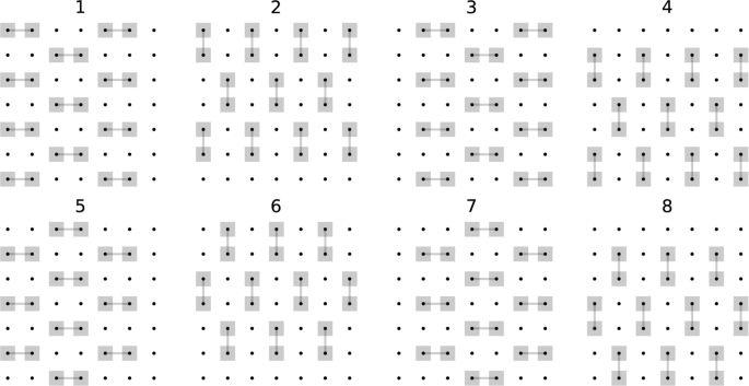

  

  Layout of two-qubit gates and the corresponding cycle order (from 1 to 8). This layout can be tiled over 2D square grids of arbitrary size. The Bristlecone architecture is a diamond-shaped subset of such a 2D grid. For our simulations, we use CZ gates as the two-qubit gate

• (3) Within these layers, for each qubit that is not being acted upon by a two-qubit gate in the current layer, and such that a two-qubit gate was acting on it in the previous layer, randomly apply (with equal probability) a gate in the set {X^1/2, Y^1/2}.

• (4) Within these layers, for each qubit that is not being acted upon by a two-qubit gate in the current layer and was acted upon by a gate in the set {X^1/2, Y^1/2, H} in the previous layer, apply a T gate.

• (5) Apply a final layer of H gates to all the qubits.

The depth of a circuit will be expressed as 1 + t + 1, where the prefix and suffix of 1 explicitly denote the presence of an initial and a final layer of Hadamard gates.

For our simulations, as was done in prior RQC works, we use the CZ gate as our two-qubit gate. One of the differences between the original prescription¹³ and this new prescription²⁸ for the generation of RQCs is that we now avoid placing T gates after CZ gates. If a T gate follows a CZ gate, this structure can be exploited to effectively reduce the computational cost to simulate the RQCs, as was done in refs. ^34,38,39. The revised RQC formulation ensures that each T gate is preceded by a {X^1/2, Y^1/2, H} gate, which foils this exploit. In addition, the layers of two-qubit gates have been reordered, to avoid consecutive “horizontal” or “vertical” layers, which is known to make simulations easier. Finally, it is important to keep the final layer of H gates, as otherwise multiple two-qubit gates at the end of the circuit can be simplified away, making the simulation easier.¹³

Replacing CZ gates with iSWAP = (|00〉〈00| + |11〉〈11| + i|01〉〈10| + i|10〉〈01|) gates is known to make the circuits yet harder to simulate. More precisely, an RQC of depth 1 + t + 1 with CZ gates is equivalent, in terms of simulation cost, to an RQC of depth 1 + t/2 + 1 with iSWAPs. In future work, we will benchmark our approach on these circuits as well.

Overview of the simulator

A given quantum circuit can always be represented as a tensor network, where one-qubit gates are rank-2 tensors (tensors of 2 indexes with dimension 2 each), two-qubit gates are rank-4 tensors (tensors of 4 indexes with dimension 2 each), and in general n-qubit gates are rank-2n tensors. The computational and memory cost for the contraction of such networks is exponential with the number of open indexes and, for large enough circuits, the network contraction is unpractical; nonetheless, it is always possible to specify input and output configurations in the computational basis through rank-1 Kronecker deltas over all qubits, which can vastly simplify the complexity of the tensor network. This representation of quantum circuits gives rise to an efficient simulation technique, first introduced in ref. ³⁶, where the contraction of the network gives amplitudes of the circuit at specified input and output configurations.

Our approach allows the calculation of amplitudes of RQCs through the contraction of their corresponding tensor networks, as discussed above, but with an essential first step, which we now describe. One of the characteristics of the layers of CZ gates shown in Fig. 4 is that it takes eight cycles for each qubit to share one, and only one, CZ gate with each of its neighbors. This property holds for all subsets of a 2D square grid, including the Bristlecone architecture. Therefore, it is possible to contract every eight layers of the tensor network corresponding to an RQC of the form described in “Revised set of RQCs” onto an I × J 2D grid of tensors, where I and J are the dimensions of the grid of qubits. Although in this work we assume that the number of layers is a multiple of 8, our simulator can be trivially used for RQCs with a depth that is not a multiple of 8. The bond dimensions between each tensor and its neighbors are the Schmidt rank of a CZ gate, which (as for any diagonal two-qubit gate) is equal to 2 (note that for iSWAP the Schmidt rank is equal to 4, thus effectively doubling the depth of the circuit as compared with the CZ case). After contracting each group of eight layers in the time direction onto a single, denser layer of tensors, the RQC is mapped onto an I × J × K three-dimensional grid of tensors of indexes of bond dimension 2, as shown in Fig. 5, where K = t/8, and 1 + t + 1 is the depth of the circuit (see “Revised set of RQCs”). It is noteworthy that the initial (final) layer of Hadamard gates, as well as the input (resp. output) delta tensors, can be trivially contracted with the initial (resp. final) cycle of eight layers of gates. At this point, the randomness of the RQCs appears only in the entries of the tensors in the tensor network, but not in its layout, which is largely regular, and whose contraction complexity is therefore independent of the particular RQC instance at hand. This approach contrasts with those taken in refs. ^34,37,39, which propose simulators that either benefit from an approach tailored for each random instance of an RQC, or take advantage of the particular layout of the CZ layers.

Fig. 5

(a) 3D grid of tensors obtained by contracting eight consecutive layers of CZ gates, including the single-qubit gates. (b) Example of a typical block of eight layers of gates on a single qubit; note that the qubit shares one CZ gate with each of its four neighbors per block

The contraction of the resulting 3D tensor network described above (see Fig. 5), to compute the amplitude corresponding to specified initial and final bit-strings is described in the following “Contraction of the 3D tensor network”.

Contraction of the 3D tensor network

In this section, we describe the contraction procedure followed for the computation of single perfect-fidelity output amplitudes for the 3D grid of tensors described in the previous section.

Starting from the 3D grid of tensors of Fig. 5, we first contract each vertical (K direction) column of tensors onto a single tensor of at most four indexes of dimension 2^K each (see left panel of Fig. 6). It is noteworthy that for the circuit sizes and depths we simulate, K is always smaller than I and J, and so this contraction is always feasible in terms of memory, fast, and preferable to a contraction in either the direction of I or J. This results in a 2D grid of tensors of size I × J, where all indexes have dimension 2^K (see the right panel of Fig. 6). It is worth noting that contracting in the time direction first is done at a negligible cost and reduces the number of high-complexity contractions to only the ones left in the resulting 2D grid.

Fig. 6

a Contraction of the 3D grid of tensors (see Fig. 5) in the time direction to obtain (b) a 2D grid of tensors

Although we have focused so far on the steps leading to the 2D square grid tensor network of Fig. 6, it is easy to see that the Bristlecone topology (see Bristlecone-72 in Fig. 1) is a sub-lattice of a square grid or qubits, and so all considerations discussed up to this point are applicable. Even though Bristlecone has 72 qubits, the top-left and bottom-right qubits of the network can be contracted trivially with their respective only neighbor, adding no complexity to our classical simulation of RQCs. For this reason, without loss of generality, we “turn off” those two qubits from the Bristlecone lattice and work only with the resulting sub-lattice, which we call Bristlecone-70 (see Fig. 1). For the remainder of this section, we will focus on Bristlecone-70 and other sub-lattices of Bristlecone (see sub-lattices considered in Fig. 1), and we will refer back to square grids of qubits in later sections.

Cutting indexes and the contraction of the 2D tensor network

From Fig. 1, it is easy to see that it is not possible to contract the Bristlecone-70 tensor network without generating tensors of rank 11, where each index has dimension 2^K. For a circuit of depth 1 + 32 + 1 and K = 4, the dimension of the largest tensors is 2^11×4, which needs over 140 TB of memory to be stored using single precision floating point complex numbers, far beyond the RAM of a typical HPC cluster node (between 32 GB and 512 GB). Therefore, to avoid the memory bottleneck, we decompose the contraction of the Bristlecone-70 tensor network into independent contractions of several easier-to-compute sub-networks. Each sub-network is obtained by applying specific “cuts”, as is described below.

Given a tensor network with n tensors and a set of indexes to contract {i_l}_{l = 1,…}, $\mathop {\sum}\nolimits_{i_1,i_2, \ldots } {T^1} T^2 \ldots T^n$, we define a cut over index i_k as the explicit decomposition of the contraction into $\mathop {\sum}\nolimits_{i_k} {\left( {\mathop {\sum}\nolimits_{\{ i_l\} _{l = 1, \ldots } - \{ i_k\} } {T^1} T^2 \ldots T^n} \right)}$. This implies the contraction of dim(i_k) many tensor networks of lower complexity, namely each of the $\mathop {\sum}\nolimits_{\{ i_l\} _{l = 1, \ldots } - \{ i_k\} } {T^1} T^2 \ldots$ networks, where tensors involving index i_k decrease their rank by 1, fixing the value of i_k to the particular value given by the term in $\Sigma _{i_k}$. This procedure, equivalent to the ones used in refs. ^28,34,38,39 reduces the complexity of the resulting tensor network contractions to computationally manageable tasks (in terms of both memory and time), at the expense of creating exponentially many contractions. The resulting tensor networks can be contracted independently, which results in a computation that is embarrassingly parallelizable. It is possible to make more than one cut on a tensor network, in which case i_k refers to a multi-index; the contribution to the final sum of each of the contractions (each of the values of the multi-index cut) is called a “path” and the final value of the contraction is the sum of all path contributions.

For the Bristlecone-70 example with depth (1 + 32 + 1), making four cuts, as shown in Fig. 7(a), decreases the size of the maximum tensor stored during the contraction from 2^11×4 to 2^7×4 entries, at the price of 2^4×4 contractions to be computed. At the same time, the choice of cuts aims at lowering the number of high-complexity contractions needed per path, as well as lowering the number of largest tensors held simultaneously in memory. It is noteworthy that for Bristlecone-60, tensors A and B are both equally large, and that the number of high-complexity contractions is larger than for a single path of Bristlecone-70.

Fig. 7

(a) Sketch of the contraction procedure followed to obtain one path of one amplitude of the Bristlecone-70 with depth (1 + 32 + 1). We first make four cuts of dimension 2⁴ each, leaving us with 2¹⁶ paths; for each path, we contract all tensors on region A and all tensors on region B; then tensors A and B are contracted together; finally, tensor C (which is independent of chosen path and can in addition be computed very efficiently) is contracted with AB, which obtains the contribution of this path to this particular amplitude. (b) Corresponding regions A, B, and C for the Bristlecone-24, -48, -60, and -64. It is worth noting that both the Bristlecone-48 and the Bristlecone-64 need 2 cuts of dimension 2⁴ each, whereas the Bristlecone-60 needs 3 of such cuts, making it a factor of 2⁴ times harder than Bristlecone-64, even though it has 4 qubits less

After making these cuts, the contraction of each path is carried out in the following way (see Fig. 7): first, we contract all tensors within region A onto a tensor of rank 7 (tensor A); we do the same for tensor B; then tensors A and B are contracted onto a rank-6 tensor, AB; finally, tensor C is contracted, which does not depend on the particular path at hand, followed by the contraction of AB with C onto a scalar. In Fig. 7(b), we depict the corresponding A, B, and C regions for the sub-lattices of Bristlecone we use in our simulations, as well as the cuts needed to contract the resulting tensor networks using the described method, in particular for Bristlecone-48, -60, and -64. It is noteworthy that Bristlecone-48 and -64 need both two cuts of depth 4, making them similar to each other in complexity, whereas Bristlecone-60 needs three cuts, making it substantially harder to simulate.

We identify a family of sub-lattices of Bristlecone, namely Bristlecone-24, -30, -40, -48, -60, and -70, which are hard to simulate classically, while keeping the number of qubits and gates as low as possible. Indeed, the fidelity of a quantum computer decreases with the number of qubits and gates involved in the experiment,¹³ and so finding classically hard sub-lattices with a small number of qubits is essential for quantum supremacy experiments. It is interesting to observe that Bristlecone-64 is an example of a misleadingly large lattice that is easy to simulate classically (see "Results" for our numerical results).

It is noteworthy that the rules for generating RQCs cycle over the layers of two-qubit gates depicted in Fig. 4. In the case that the cycles or the layers are perturbed, our simulator can be trivially adapted. In particular: (1) if the layers are applied in a different order, but the number of two-qubit gates between all pairs of neighbors is the same, then the 2D grid tensor network of Fig. 6 still holds and the contraction method can be applied as described; (2) if there is a higher count of two-qubit gates between some pairs of neighbors than between others, then the corresponding anisotropy in the bond dimensions of the 2D tensor network can be exploited through different cuts.

Remarks on the choice of cuts and contraction ordering

The cost of contracting a tensor network depends strongly on the contraction ordering chosen and is a topic covered in the literature (see refs. ^36,37); determining the optimal contraction ordering is an Non-deterministic Polynomial (NP)-hard problem. Given an ordering, the leading term to the time complexity of the contraction is given by the most expensive contraction between two tensors encountered along the contraction of the full network; the optimal ordering given this cost model is closely related to the treewidth of the line-graph of the tensor network. However, a more practical approach to determining the cost of a particular contraction ordering is the FLOP count of the contraction of the entire network (i.e., the number of scalar additions and multiplications needed); this accounts for cases where a single high-complexity contraction is preferable to a large number of low-complexity ones. The latter cost model is commonly used, to determine the optimal ordering for the contraction of tensor networks (e.g., in ref. ³⁹). It is noteworthy that, although the choice of a contraction ordering affects also its memory complexity, by what we mean the memory required to perform the contraction, this is usually a smaller concern as compared with time complexity.

An even more realistic approach needs to consider the performance efficiency of the different tensor contractions, i.e., the delivered FLOP/s of each contraction. In particular, modern computing architectures benefit from high arithmetically intensive contractions, i.e., contractions with a large ratio between the FLOP count and the number of reads and writes from and to memory. Highly unbalanced matrix multiplications, e.g., present low arithmetic intensity, whereas the multiplication of large squared matrices shows high arithmetic intensity, and therefore achieves a performance very close to the theoretical peak FLOP/s of a particular CPU. This principle (which prioritizes time-to-solution over FLOP count-to-solution) is at the heart of our choice to contract the quantum circuits first into blocks and subsequently along the “time” direction. This choice, beyond “regularizing” the tensor network, serves two purposes, aimed at decreasing the overall time-to-solution in practice: (1) the vast majority of contractions are performed in these first steps and are done in a negligible amount of time, leaving most of the computation to a small number of subsequent high-complexity contractions; and (2) the remaining high-complexity contractions have high arithmetic intensity and therefore achieve high efficiency. In addition, contracting all blocks in the time direction first reduces the memory requirement of the subsequent contraction as compared with keeping the tensor network in its three-dimensional version.

The cost model discussed here becomes more intricate when cuts are considered. Each choice of cuts not only has a different impact on the memory complexity of the resulting, simplified tensor networks, but it can also substantially affect their time complexity. As was explained in “Contraction of the 3D tensor network,” the main purpose of the cuts is reducing the memory requirement of the resulting contractions to fit the limits of each computation node; this is indeed the main factor taken into account when choosing a set of cuts. However, the right choice of cuts can also allow us to, again, have a small number of high arithmetic intensity contractions. This is the case with the contractions depicted in Fig. 7, where the main bottleneck is given by the contraction of A with B, which is very arithmetically intensive; see also Fig. A1 for an example on a square lattice.

Finally, it is worth noting the two more factors on the runtime of a contraction. First, if the memory requirement of a contraction is well below the limits of a computing node, then several contractions can be run in parallel. In these cases, there is a trade-off between the number of cuts made and the number of contractions run in parallel. Second, the choice of cuts can affect the number of tensors reused across different paths (which is done at a memory cost), which can have a substantial impact on the computation time of an amplitude, as can be seen in the examples of Supplementary Information A.

Although a cost model involving all the factors discussed above can be well characterized, automatically optimizing the cuts chosen and the contraction ordering, together with the tensors reused across paths, is beyond the scope of this work. In practice, we study different configurations “by hand”. It is noteworthy that, once the tensor networks have a certain level of regularity, it is not hard to make a choice that is close to optimal.

Implementation of the simulator

We implemented our tensor network contraction engine for CPU-based supercomputers using C⁺⁺. We have planned to release our tensor contraction engine in the near future. During the optimization, we were able to identify two clear bottlenecks in the implementation of the contractions: the matrix multiplication required for each index (or multi-index) contraction and the reordering of tensors in memory needed to pass the multiplication to a matrix multiplier in the appropriate storage order (in particular, we always use row-major storage). In addition, to avoid time-consuming allocations during the runs, we immediately allocate large-enough memory to be reused as scratch space in the reordering of tensors and other operations.

Matrix multiplications with Intel® MKL

For the multiplication of two large matrices that are not distributed over several computational nodes, Intel’s MKL library is arguably the best performing library on Intel CPU-based architectures. We therefore leave this essential part of the contraction of tensor networks to MKL’s efficient, hand-optimized implementation of the Basic Linear Algebra Subprograms (BLAS) matrix multiplication functions. It is worth noting that, even though we have used MKL, any other BLAS implementation could be used as well and other linear algebra libraries could be used straightforwardly.

Cache-efficient index permutations

The permutation of the indexes necessary as a preparatory step for efficient matrix multiplications can be very costly for large tensors, as it involves the reordering of virtually all entries of the tensors in memory; similar issues have been an area of study in other contexts.^45,46,47 In this section we describe our novel cache-efficient implementation of the permutation of tensor indexes.

Let A_i0,…,ik be a tensor with k indexes. In our implementation, we follow a row-major storage for tensors, a natural generalization of matrix row-major storage to an arbitrary number of indexes. In the tensor network literature, a permutation of indexes formally does not induce any change in tensor A. However, given a storage prescription (e.g., row-major), we will consider that a permutation of indexes induces the corresponding reordering of the tensor entries in memory. A naive implementation of this reordering routine will result in an extensive number of cache misses, with poor performance.

We implement the reorderings in a cache-efficient way by designing two reordering routines that apply to two special index permutations. Let us divide a tensor’s indexes into a left and a right group: $A\underbrace{i_0, \ldots ,i_j}\underbrace {i_{j + 1}, \ldots ,i_k}$. If a permutation involves only indexes in the left (right) group, then the permutation is called a left (resp. right) move. Let γ be the number of indexes in the right group. We will denote the left (resp. right) moves with γ indexes in the right group by Lγ (resp. Rγ). The importance of these moves is that they are both cache-efficient for a wide range of values of γ, and that an arbitrary permutation of the indexes of a tensor can be decomposed into a small number of the left and right moves, as will be explained later in this section. Let d_γ be the dimension of all γ right indexes together. Then the left moves involve the reordering across groups of d_γ entries of the tensor, where each group of d_γ entries is contiguous in memory and is moved as a whole, without any reordering within itself, therefore largely reducing the number of cache misses in the routine. On the other hand, right moves involve reordering within all of d_γ entries that are contiguous in memory, but involves no reordering across groups, hence greatly reducing the number of cache misses, as all reorderings take place in small contiguous chunks of memory. Figure 8 shows the efficiency of Rγ and Lγ as compared with a naive (but still optimized) implementation of the reordering that is comparable in performance to python’s numpy implementation. A further advantage of the left and right moves is that they can be parallelized over multiple threads and remain cache-efficient in each of the threads. This allows for a very efficient use of the computation resources, while the naive implementation does not benefit from multithreading.

Fig. 8

Single thread computation times on Broadwell nodes on Pleiades for an arbitrary permutation of the indexes of a tensor of single precision complex entries (and 25 indexes of dimension 2 each) following an optimized, naive implementation of the reordering (green), an arbitrary Lγ move (red), and an arbitrary Rγ move (blue). The optimized, naive approach performs comparably to python’s numpy implementation of the reordering. It is noteworthy that, for a wide range of γ, the left and right moves are very efficient. Left inset: zoomed version of the main plot. For γ ∈ [5; 10] both the right and left moves are efficient. Right inset: computation times for L5 and R10 (used in practice) as a function of the number of threads used

Let us introduce the decomposition of an arbitrary permutation into the left and right moves through an example. Let A_abcdefg be a tensor with seven indexes of dimension d each. Let abcde fg → c f eadgb be the index permutation we wish to perform. Furthermore, let us assume that it is known that L2 and R4 are cache efficient. Let us also divide the list of seven indexes of this example in three groups: the last two (indexes 6 and 7), the next group of two indexes from the right (indexes 4 and 5), and the remaining three indexes on the left (1, 2, and 3). We now proceed as follows. First, we apply an L2 move that places all indexes in the left and middle groups that need to end up in the rightmost group in the middle group; in our case, this is index b and the L2 we have in mind is $\underbrace {abc|de}_{L2}|fg \to \underbrace {cae|bd}_{L2}|fg$; it is noteworthy that if the middle group is at least as big as the rightmost group, then it is always possible to do this. Second, we apply an R4 move that places all indexes that need to end up in the rightmost group in their final positions; in our case, that is $cae|\underbrace {bd|fg}_{R4} \to cae|\underbrace {fd|gb}_{R4}$; note that, if the first move was successful, then this one can always be done. Finally, we take a final L2 move that places all indexes in the leftmost and middle groups in their final positions, i.e., $\underbrace {cae|fd}_{L2}|gb \to \underbrace {cfe|ad}_{L2}|gb$. We have decomposed the permutation into three cache-efficient moves, Lμ − Rν − Lμ, with μ = 2, ν = 4. It is worth noting that it is essential for this particular decomposition that the middle group has at least the same dimension as the rightmost group. It is also crucial that both Lμ and Rν are cache efficient.

In practice, we find that (beyond the above example, where μ = 2 and ν = 4) for tensors with binary indexes, μ = 5 and ν = 10 are good choices for our processors (see Fig. 8). If the tensor indexes are not binary, this approach can be generalized: if all indexes have a dimension that is a power of 2, then mapping the reordering onto one involving explicitly binary indexes is trivial; in the case where indexes are not all powers of 2, then different values of μ and ν could be found, or decompositions more general than Lμ − Rν − Lμ could be thought of. In our case, we find good results for the L5 − R10 − L5 decomposition. Note also that in many cases a single R or a single L move is sufficient, and sometimes a combination of only two of them is enough, which can accelerate contractions by a large factor.

We apply a further optimization to our index permutation routines. A reordering of tensor entries in memory (either a general one or some of Rγ or Lγ moves) involves two procedures: generating a map between the old and the new positions of each entry, which has size equal to the dimension of all indexes involved and applying the map to actually move the entries in memory. The generation of the map takes a large part of the computation time, and so storing maps that have already been used in a look-up table (memoization), to reuse them in future reorderings, is a desirable technique to use. Although the size of such maps might make this approach impractical in general, for the left and right moves memoization becomes feasible, as the size of the maps is now exponentially smaller than in the general case due to the left and right moves only involving a subset of indexes. In the contraction of regular tensor networks we work with maps reappear often, and so memoization proves very useful.

The implementation of the decomposition of general permutations of indexes into the left and right moves, with all the details discussed above, give us speedups in the contractions that range from under 5% in single-threaded contractions that are dominated by matrix multiplications, to well over 50% in multithreaded contractions that are dominated by reorderings. A detailed comparison of runtimes using a naive approach and the cache-efficient approach discussed is shown in Fig. 9. The contraction corresponding to the simulation of Bristlecone-60 with depth 1 + 32 + 1 (presented in “Contraction of the 3D tensor network”) is dominated by reorderings, as a large part of the runtime is spent in building tensor A, which involves a large number of “unbalanced” contractions, where the reordering of a large tensor is followed by the multiplication of a large matrix with a small one. The contraction corresponding the a 7 × 7 grid of depth 1 + 40 + 1 (presented in Supplementary Information A) is dominated by a few “balanced” contractions of large tensors and so the overall runtime is dominated by matrix–matrix multiplication. In this case, larger speedups are still achieved using a large number of threads, due to multithreading, and the speedup using a single thread is appreciable but small; in practice, we use 13 threads per job on Skylake nodes, where we can only fit 3 jobs per node due to memory constraints, and a larger number of threads per job on other node types. Finally, it is worth mentioning that runtimes are still robust when using cache-efficient, multithreaded index permutations, showing small variation among runs.

Fig. 9

Comparison of the runtime of the computation of an amplitude using a naive index permutation implementation (comparable to python’s numpy implementation) and the cache-efficient implementation described in “Implementation of the simulator,” using Skylake nodes on Electra. Left: computation of three paths of an amplitude of Bristlecone-60 with depth 1 + 32 + 1, corresponding to a target fidelity f = 3/2¹² (see “Results”). Right: computation of three paths of an amplitude of a grid of size 7 × 7 with depth 1 + 40 + 1, corresponding to a target fidelity f = 3/2¹⁰ (see also “Results”). Runtimes using a varying number of threads (one threads per physical core) in an otherwise idle node are presented (single job), as well as runtimes for the case where several amplitudes are computed on the same node, fitting as many concurrent computations as possible (concurrent jobs, also shown in the insets for clarity), a number that is constrained by memory requirements; the latter is the case for the simulations presented in “Results”. Cache-efficient runs show always better runtimes. The scaling of runtime with number of threads is better for the cache-efficient runs, given multithreading; note that the matrix–matrix multiplication part of the contraction is always multithreaded. Concurrent jobs suffer from contention, which is larger for the cache-efficient runs, presumably due to a larger use of bandwidth; however, runtimes are still substantially improved in this case

Fast sampling of bit-strings from low-fidelity RQCs

Although the computation of perfect fidelity amplitudes of output bit-strings of RQCs is needed for the verification of quantum supremacy experiments,¹³ classically simulating sampling from low-fidelity RQCs is essential to benchmark the performance of classical supercomputers in carrying out the same task as a noisy quantum computer. Indeed, present day quantum computers suffer from noise and errors in each gate. In the commonly used digital error model,^{13,48,49,50,51,52,53} the total error probability for a RQC is the sum of the probability of error from each gate. The fidelity, or probability of no errors, of a quantum computer or of a classical algorithm for RQC sampling can be estimated with XEB.¹³ Therefore, we only require the same value for the cross-entropy or fidelity in the classical algorithm as in the noisy quantum computer. A superconducting quantum processor with the present day technology is expected to achieve a fidelity of around 0.5% for circuits with the number of gates considered here.¹³

In “Simulating low delity RQCs,” we describe two methods to mimic the fidelity f of the output wavefunction of the quantum computer with our simulator, providing a speedup of a factor of 1/f to the simulation as compared with the computation of exact amplitudes.²⁸ Both methods can be adjusted to provide the same fidelity and therefore the same cross-entropy,¹³ as a noisy quantum computer. That is, they result in an equivalent RQC sampling. In “Fast sampling technique,” we describe a way to reduce the computational cost of the sampling procedure on tensor contraction type simulators by a factor of almost 10×, under reasonable assumptions. Finally, in “Sampling from a non fully-thermalized Porter-Thomas distribution,” we discuss the implications of sampling from a Porter–Thomas distribution that has not fully converged.

Simulating low-fidelity RQCs

Here we describe two methods to reduce the computational cost of classical sampling from an RQC given a target fidelity.

Summing a fraction of the paths

This method, presented in ref. ²⁸, exploits the fact that, for RQCs, the decomposition of the output wavefunction of a circuit into paths $\left| \psi \right\rangle = \mathop {\sum}\nolimits_{p \in \{ paths\} } {|\psi _p\rangle }$ (see “Contraction of the 3D tensor network”) leads to terms |ψ_p〉 that have similar norm and that are almost orthogonal to each other. For this reason, summing only over a fraction f of the paths, one obtains a wavefunction $|\tilde \psi \rangle$ with norm $\langle \tilde \psi |\tilde \psi \rangle = f$. Moreover, $|\tilde \psi \rangle$ has fidelity f as compared with |ψ〉, that is:

$$\left| {\frac{{\langle \psi |\tilde \psi \rangle }}{{\sqrt {\langle \tilde \psi |\tilde \psi \rangle } }}} \right|^2 = f.$$

(1)

Therefore, amplitudes of a fidelity f wavefunction can be computed at a cost that is only a fraction f of that of the perfect fidelity case.

We find empirically that, although the different contributions |ψ_p〉 fulfill the orthogonality requirement (with a negligible overlap; e.g., in the Bristlecone-60 simulation, the mutual fidelity between pairs out of 4096 paths is about 10⁻⁶), there is some non-negligible variation in their norms (see “Results” and Fig. 10), and thus the fidelity achieved by |ψ_p〉 is equal to:

$$\left| {\frac{{\langle \psi |\psi _p\rangle }}{{\sqrt {\langle \psi _p|\psi _p\rangle } }}} \right|^2 = \langle \psi _p|\psi _p\rangle ,$$

(2)

which is in general different than (#paths)⁻¹. If an extensive subset of paths is summed over, then the variations on the norm and the fidelity are suppressed, and the target fidelity is achieved. This was the case in ref. ²⁸. However, in this work we aim at minimizing the number of cuts on the circuits and so low-fidelity simulations involve a small number of paths (between 1 and 21 in the cases simulated). In this case, some “unlucky” randomly selected paths might contribute with a fidelity that is below the target, whereas others might achieve a higher fidelity than expected.

Fig. 10

Porter–Thomas distribution for the three different sub-lattices of Bristlecone simulated with depth (1 + 32 + 1). (a) Bristlecone-64 ([Run 1]); 1.2 × 10⁶ amplitudes with a target fidelity f = 0.78%; $\langle \tilde \psi |\tilde \psi \rangle = 0.87f$. (b) Bristlecone-48 ([Run 2]); 1.2 × 10⁶ amplitudes with target fidelity f = 0.78%; $\langle \tilde \psi |\tilde \psi \rangle = 0.77f$. (c) Bristlecone-60 ([Run 6]); 1.15 × 10⁶ amplitudes with a target fidelity f = 0.51%; $\langle \tilde \psi |\tilde \psi \rangle = 1.38f$. For reference, the theoretical value of the Porter–Thomas distribution is plotted (solid line). For some simulations, the depth is not sufficient to fully converge to a Porter–Thomas distribution. Furthermore, summing a small number of paths of low fidelity might lead to worse convergence than expected for a particular depth (see “Simulating low delity RQCs”)

Finally, the low-fidelity probability amplitudes reported in ref. ²⁸, obtained using the method described above, follow a Porter–Thomas distribution as expected for perfect fidelity amplitudes. Again, this is presumably true only in the case when a large number of paths is considered. In our case, we find distributions that have not fully converged to a Porter–Thomas, but rather have a larger tail (see "Results" and Fig. 10). We attribute this phenomenon to the cuts in the circuit acting as removed gates between qubits, thus increasing the effective diameter of the circuit, which needs higher depth to fully thermalize. We discuss the implications of these tails for the sampling procedure in “Sampling from a non fully-thermalized Porter–Thomas distribution.”

Fraction of perfect fidelity amplitudes

There exists a second method to simulate sampling from the output wavefunction |ψ〉 with a target fidelity f that avoids summing over a fraction of paths.

The output density matrix of a RQC with fidelity f can be written as¹³

$$\rho = f|\psi \rangle \langle \psi | + (1 - f)\frac{1}{N}.$$

(3)

This means that to produce a sample with fidelity f we can sample from the exact wavefunction |ψ〉 with probability f or produce a random bit-string with probability 1 − f. The sample from the exact wavefunction can be simulated by calculating the required number of amplitudes with perfect fidelity.

It is noteworthy that the method presented in this section involves the computation of the same number of paths as the one described in “Simulating low delity RQCs” for a given f, circuit topology, circuit depth, and set of cuts. However, this second method is more robust in achieving a target fidelity. Note that by this argument the 6000 amplitudes of [Run 5] are equivalent to 1.2 M amplitudes at 0.5% fidelity.

It is also noteworthy that, even though this method and the one presented in “Simulating low delity RQCs” have the same computational cost for tensor network-based simulators, for Schrödinger–Feynman simulators such as the one presented in ref. ²⁸ it is preferable to consider a fraction of paths as opposed to a fraction of perfect fidelity amplitudes. This is due to the small cost overhead of computing an arbitrary number of amplitudes using these simulators.

Fast sampling technique

Although 10⁶ sampled amplitudes are necessary for cross-entropy verification of the sampling task,¹³ the frugal rejection sampling proposed in ref. ²⁸ needs the numerical computation of 10 × 10⁶ = 10⁷ amplitudes, to carry out the correct sampling on a classical supercomputer. This is due to the acceptance of 1/M amplitudes (on average) of the rejection sampling, where M = 10 when sampling from a given Porter–Thomas distribution with statistical distance ε of the order of 10⁻⁴ (negligible).

In this section, we propose a method to effectively remove the 10× overhead in the sampling procedure for tensor network-based simulators, which normally compute one amplitude at a time. For the sake of clarity, we tailor the proposed fast sampling technique to the Bristlecone architecture. However, it can be straightforwardly generalized to different architectures (see Supplementary Information A). Given the two regions of the Bristlecone (and sub-lattices) AB and C of Fig. 7, and the contraction proposed (see “Contraction of the 3D tensor network”), the construction of tensor C and its subsequent contraction with AB are computationally efficient tasks done in a small amount of time as compared with the full computation of the particular path. This implies that one can compute, for a given output bit-string on AB, s_AB, a set of 2¹² amplitudes generated by the concatenation of s_AB with all possible s_C bit-strings on C at a small overhead cost per amplitude. We call this set of amplitudes a “batch”; we denote its size by N_C and each of the (concatenated) bit-strings by s_ABC. In practice, we find that for the Bristlecone-64 and -60 with depth (1 + 32 + 1), the computation of a batch of 30 amplitudes is only around 10% more expensive than the computation of a single amplitude, whereas for the Bristlecone-48 and -70 with depth (1 + 32 + 1), the computation of a batch of 256 amplitudes is around 15% more expensive than the computation of a single amplitude, instead of a theoretical overhead of 30× and 256×, respectively.

The sampling procedure we propose is a modification of the frugal rejection sampling presented in ref. ²⁸ and proceeds as follows. First, we choose slightly over 10⁶ (see below) random bit-strings on AB, s_AB. For each s_AB, we choose N_C bit-strings on C, s_C, at random (without repetition). We then compute the probability amplitudes corresponding to all s_ABC bit-strings on all (slightly over) 10⁶ batches. We now shuffle each batch of bit-strings. For each batch, we proceed onto the bit-strings in the order given by the shuffle; we accept a bit-string s_ABC with probability min [1, p(s_ABC)N/M], where p(s_ABC) is the probability amplitude of s_ABC and N is the dimension of the Hilbert space; once a bit-string is accepted, or the bit-strings of the batch have been exhausted without acceptance, we proceed to the next batch. By accepting at most one bit-string per batch, we avoid introducing spurious correlations in the final sample of bit-strings.

Given an M and a batch size N_C, the probability that a bit-string is accepted from a batch is (on average) ${1-(1-1/M)^{N_C}}$. For M = 10 and N_C = 30, the probability of acceptance in a batch is 95.76% and one would need to compute amplitudes for 1.045 × 10⁶ batches, to sample 10⁶ bit-strings; for M = 10 and N_C = 60, the probability goes up to 99.82% and one only needs 1.002 × 10⁶ batches; for M = 10 and N_C = 256, the probability of acceptance is virtually 100% and 1.00 × 10⁶ batches are sufficient. There is an optimal point, given by the overhead in computing batches of different sizes N_C and the probability of accepting a bit-string on a batch given N_C, which minimizes the runtime of the algorithm.

There is a crucial condition for this sampling algorithm to work, namely the absence of correlations between the probability amplitudes of the bit-strings {s_ABC} for fixed s_AB, so that they are indistinguishable from probability amplitudes taken from random bit-strings over ABC. We expect this condition to be satisfied for chaotic systems that have converged to a Porter–Thomas distribution. To test this, we perform the following test: for Bristlecone-24, we choose 1000 bit-strings over AB (s_AB) at random and for each of them we generate a batch of size N_C = 32, where we constrain the bit-strings {s_C} to be the same across batches. We now compute the Pearson’s correlation coefficient between the two sets of 1000 amplitudes gotten for each pair of bit-strings in C and we do this for all 32 × 31/2 pairs. If the probability amplitudes of each batch are really uncorrelated to each other, we expect the correlation coefficient to vanish. We show the coefficient as a function of Hamming distance between the pairs in Fig. 11 (a) and (b). We can see that, for depth (1 + 24 + 1) (a) there is a small but non-negligible correlation, which in fact decreases on average with Hamming distance. For depth (1 + 32 + 1) (b), the correlation is Hamming distance independent and approaches zero. In Fig. 11(b), we compare the distribution of Pearson’s coefficients obtained for both depths analyzed to that one obtained from pairs of sets of size 1000 sampled from a Porter–Thomas distribution. Although a fairer comparison would involve sampling from the distribution of the output wavefunction of the RQC, which might differ from the Porter–Thomas in the absence of convergence, we still see a clear tendency of the distributions to match for longer depth, i.e., closer to convergence.

Fig. 11

(a)-(b) Pearson’s coefficient as a function of Hamming distance for pairs generated at random on subsystem C of sub-lattice Bristlecone-24, for samples of size 1000 of random strings on subsystem A + B. All pairs between strings of a set of 32 random strings on subsystem C are considered. The average and SD (error bars) for each Hamming distance is plotted with a solid line. We can see that, for depth (1 + 24 + 1) (a), the system has not thermalized and the correlation decreases with Hamming distance; for depth (1 + 32 + 1) (b), correlations approach zero and become Hamming distance independent (on subsystem C). (c) we compare the distribution of Pearson’s coefficients, obtained as described above, to the distribution of Pearson’s coefficients obtained (numerically) from probability amplitudes with the same sample size as in the simulations above, drawn from a Porter–Thomas distribution. At large-enough depth, the system is expected to thermalize and the two distributions match, meaning that the probability amplitudes obtained by varying bit-strings only on subsystem C are uncorrelated

Sampling from a non-fully thermalized Porter–Thomas distribution

In ref. ²⁸, an error of the order of 10⁻⁴ is computed for a frugal rejection sampling with M = 10, assuming Porter–Thomas statistics. When the distribution has not converged to a Porter–Thomas, but rather has a larger tail, we expect the error to increase. We can estimate the error in sampling numerically for the cases simulated here as the sum of the probability amplitudes larger than M/N with N being the dimension of the Hilbert space, multiplied by N and divided by the number of amplitudes computed. For M = 10, we estimate an error ε = 9.3 × 10⁻⁴ for [Run 1], ε = 1.0 × 10⁻² for [Run 2], and ε = 2.5 × 10⁻³ for [Run 6], respectively. If instead we consider M = 15, this lowers the error to ε = 1.3 × 10⁻⁵ for [Run 1], ε = 1.0 × 10⁻³ for [Run 2], and ε = 1.15 × 10⁻⁴ for [Run 6], respectively. Increasing M, to reduce the error in the frugal sampling, implies a lower acceptance rate in the fast sampling, which is resolved by increasing the size of the batches N_C, which is done at a small cost.

Simulation of Bristlecone compared with rectangular grids

The diamond shape of the topology of Bristlecone and its hard sub-lattices (see Fig. 1: Bristlecone-24, -30, -40, -48, -60, and -70) makes them particularly hard to simulate classically when compared with rectangular grids of the same (or smaller) number of qubits. Indeed, these lattices are subsets of large rectangular grids, from which they inherit their diameter; e.g., Bristlecone-70 is a sub-lattice of a 10 × 11 grid. When cutting the lattice (see “Contraction of the 3D tensor network”), one has to apply several cuts, to decrease the maximum size of the tensors in the contraction to manageable sizes; in the case of Bristlecone-70 and depth (1 + 32 + 1), four cuts are needed, to have tensors in the contraction of at most dimension 2^7×4, whereas for a rectangular 8 × 9 lattice (with 72 qubits) only 3 cuts are needed. It is noteworthy that the computational cost scales with the dimension of the indexes cut, i.e., exponentially with the number of cuts.

The same applies to a simulator based on a full split of the circuit into two parts, as in refs. ^12,28,38. For instance, the number of CZ gates for RQCs with depth (1 + 32 + 1), which are cut when splitting Bristlecone-60 in two halves is equal to 40. In comparison, 8 × 8 grids of qubits with the same depth have only 32 CZ gates cut. See Supplementary Information C for more details.

As was discussed in “Overview of the simulator”, identifying topologies that are hard to simulate classically, but that minimize the number of qubits involved, increases the chances of success of quantum supremacy experiments, due to the decrease of the overall fidelity of the quantum computer with the number of gates and qubits.¹³ For this reason, we find that Bristlecone is a good setup for quantum supremacy experiments.

References

Nielsen, M. A. & Chuang, I. L. Quantum Computation and Quantum Information (Cambridge Univ. Press, Cambridge, 2000).
Rieffel, E. G. & Polak, W. Quantum Computing: A Gentle Introduction. (MIT Press, Cambridge, MA, 2011).
Shor P. Algorithms for quantum computation: discrete logarithms and factoring. In Proc. 35th Annual Symposium on Foundations of Computer Science, 124–134 (IEEE, 1994).
Grover L. K., A fast quantum mechanical algorithm for database search. In Proc.28th Annual ACM Symposium on Theory of Computing - STOC ’96, 212–219 (ACM, 1996).
Feynman, R. P. Simulating {P}hysics with {C}omputers. Int. J. Theoretical Phys. 21, 467 (1982).
Aspuru-Guzik, A., Dutoi, A. D., Love, P. J. & Head-Gordon, M. Chemistry: simulated quantum computation of molecular energies. Science 309, 1704 (2005).
Babbush R., et al. Low-depth quantum simulation of materials. Phys. Rev. X 8 (2018).
Jiang, Z., Sung, K. J., Kechedzhi, K., Smelyanskiy, V. N. & Boixo, S. Quantum algorithms to simulate many-body physics of correlated Fermions. Phys. Rev. Appl. 9, 44036 (2018).
Babbush, R. et al. Encoding electronic spectra in quantum circuits with linear T complexity. Phys. Rev. X 8, 41015 (2018).
Preskill, J. Quantum computing in the NISQ era and beyond. Quantum 2, 79 (2018).
Bremner, M. J., Montanaro, A. & Shepherd, D. J. Average-case complexity versus approximate simulation of commuting quantum computations. Phys. Rev. Lett. 117, 80501 (2016).
Harrow, A. W. & Montanaro, A. Quantum computational supremacy. Nature 549, 203 (2017).
Boixo, S. et al. Characterizing quantum supremacy in near-term devices. Nat. Phys. 14, 1 (2018).
Aaronson S. & Arkhipov A. The computational complexity of linear optics. In Proc. 43rd Annual ACM Symposium on Theory of Computing, 333–342 (ACM, 2010).
Preskill, J. Quantum computing and the entanglement frontier arXiv:1203.5813 (2012).
Bremner, M. J., Montanaro, A. & Shepherd, D. J. Achieving quantum supremacy with sparse and noisy commuting quantum computations. Quantum 1, 8 (2016b).
Aaronson, S. & Chen, L. Complexity-theoretic foundations of quantum supremacy experiments. In LIPIcs-Leibniz International Proceedings in Informatics, Vol. 79 (Schloss Dagstuhl-Leibniz-Zentrum fuer Informatik, 2016).
Neill, C. et al. A blueprint for demonstrating quantum supremacy with superconducting qubits. Science 360, 195 (2018).
Bouland, A., Fefferman, B., Nirkhe, C., & Vazirani, U. On the complexity and verification of quantum random circuit sampling. Nature Physics 15, 159 (2019).
Harrow, A. & Mehraban, S. Approximate unitary $t$-designs by short random quantum circuits using nearest-neighbor and long-range gates. arXiv:1809.06957 (2018)
Movassagh, R. Efficient unitary paths and quantum computational supremacy: a proof of average-case hardness of Random Circuit Sampling. arXiv:1810.04681 (2018).
Kalai, G. & Kindler, G. Gaussian noise sensitivity and boson sampling. arXiv:1409.3093 (2014).
Arkhipov, A. Boson sampling is robust to small errors in the network matrix. Phys. Rev. A 92, 62326 (2014).
Rahimi-keshari, S. & Ralph, T. C. Sufficient conditions for efficient classical simulation of quantum optics. Phys. Rev. X 6, 1 (2016).
Yung, M. -H. & Gao, X. Can chaotic quantum circuits maintain quantum supremacy under noise? arXiv:1706.08913 (2017).
Boixo, S., Smelyanskiy, V. N. & Neven, H. Fourier analysis of sampling from noisy chaotic quantum circuits. arXiv:1708.01875 (2017).
Gao, X. & Duan, L. Efficient classical simulation of noisy quantum computation. arXiv:1810.03176 (2018).
Markov, I. L., Fatima, A., Isakov, S. V. & Boixo, S. Quantum supremacy is both closer and farther than it appears arXiv:1807.10749 (2018).
De Raedt, K. et al. Massively parallel quantum computer simulator. Comput. Phys. Commun. 176, 121 (2007).
Smelyanskiy, M., Sawaya, N. P. D., & Aspuru-Guzik, A. qHiPSTER: the quantum high performance software testing environment. arXiv:1601.07195 (2016).
Häner, T. & Steiger, D. S. Petabyte simulation of a 45-qubit quantum circuit. In Proc. International Conference for High Performance Computing, Networking, Storage and Analysis, 33 (ACM, 2017).
Pednault, E., et al, Breaking the 49-qubit barrier in the simulation of quantum circuits. arXiv:1710.05867 (2017).
De Raedt, H., et al. Massively parallel quantum computer simulator, eleven years later. Computer Physics Communications 237, 47 (2019).
Li, R., Wu, B., Ying, M., Sun, X. & Yang, G. Quantum supremacy circuit simulation on sunway TaihuLight. arXiv:1804.04797 (2018).
Bravyi, S. & Gosset, D. Improved classical simulation of quantum circuits dominated by Clifford gates. Phys. Rev. Lett. 116, 250501 (2016).
Markov, I. L. & Shi, Y. Simulating quantum computation by contracting tensor networks. SIAM J. Comput. 38, 963 (2008).
Boixo, S., Isakov, S. V., Smelyanskiy, V. N. & Neven, H. Simulation of low-depth quantum circuits as complex undirected graphical models. arXiv:1712.05384 (2017).
Chen, Z. Y. et al. 64-Qubit quantum circuit simulation. Sci. Bull. 63, 964 (2018a).
Chen, J., Zhang, F., Huang, C., Newman, M. & Shi, Y. Classical simulation of intermediate-size quantum circuits. arXiv:1805.01450 (2018).
Chen, M.-C., et al. Quantum teleportation-inspired algorithm for sampling large random quantum circuits. arXiv:1901.05003 (2019).
Guo, C., et al. General-purpose quantum circuit simulator with Projected Entangled-Pair States and the quantum supremacy frontier. arXiv:1905.08394 (2019).
Gogate, V. & Dechter, R. A complete anytime algorithm for treewidth. In Proc. CUAI, 201–208 (2004).
Jones, T., Brown, A., Bush, I. & Benjamin, S. QuEST and high performance simulation of quantum computers. Scientific Reports 9 (2019).
Boixo, S. Random quantum circuits for circuit sampling with superconducting qubits https://github.com/sboixo/GRCS.
Lokhmotov, A. & Mycroft, A. Brief announcement: optimal bit-reversal using vector permutations. In Proc. 19th ACM Symposium on Parallelism in Algorithms and Architectures (SPAA’ 07) 198–199 (2007).
Weng, T. H., Huang, S. W., Perng, R. K., Hsu, C. H. & Li, K. C. A practical openMP implementation of bit-reversal for Fast Fourier Transform. In Lecture Notes of the Institute for Computer Sciences, Social-Informatics and Telecommunications Engineering, Vol. 18 LNICST, 206–216 (Springer, 2009).
Knittel, G. QTIB: quick bit-reversed permutations on CPUs. In Proc. 17th DSP 2011 International Conference on Digital Signal Processing 1–6 (2011).
Emerson, J., Alicki, R. & Zyczkowski, K. Scalable noise estimation with random unitary operators. J. Opt. B 7, S347 (2005).
Knill, E. et al. Randomized benchmarking of quantum gates. Phys. Rev. A 77, 012307 (2008).
Magesan, E., Gambetta, J. M. & Emerson, J. Scalable and robust randomized benchmarking of quantum processes. Phys. Rev. Lett. 106, 180504 (2011).
Fowler, A. G., Mariantoni, M., Martinis, J. M. & Cleland, A. N. Surface codes: towards practical large-scale quantum computation. Phys. Rev. A 86, 032324 (2012).
Barends, R. et al. Superconducting quantum circuits at the surface code threshold for fault tolerance. Nature 508, 500 (2014).
Barends, R. et al. Digital quantum simulation of fermionic models with a superconducting circuit. Nat. Commun. 6, 7654 (2015).
Acknowledgements
We thank Edward Farhi, Bryan A. O’Gorman, Alan Ho, Sergei V. Isakov, Norman M. Tubman, and Dmitry Lyakh for enlightening discussions and Igor L. Markov for reviewing the manuscript. We also thank Orion Martin, Alan Kao, and David Yonge-Mallo for helping open source qFlex code. We thank the authors of ref. 39 for sharing the instances used in that work. We are grateful for support from NASA Ames Research Center, from the NASA Advanced Exploration Systems (AES) program, and the NASA Transformative Aeronautics Concepts Program (TACP). We also appreciate support from the AFRL Information Directorate under grant number F4HBKC4162G001. We acknowledge support of the NASA Advanced Division for providing access to the NASA HPC systems, Pleiades and Electra, during dedicated downtime. The views and conclusions contained herein are those of the authors and should not be interpreted as necessarily representing the official policies or endorsements, either expressed or implied, of the U.S. Government. The U.S. Government is authorized to reproduce and distribute reprints for governmental purpose notwithstanding any copyright annotation thereon.
Author information
Authors and Affiliations
Contributions
B.V., S.B. and S.M. designed qFlex and the study. B.V., S.B. and S.M. devised new improvements for approximated sampling. B.V. wrote the original qFlex code and B.V., B.N. and C.H. further optimized it. B.V., B.N. and C.H. ran simulations on NASA Pleiades and Electra. B.V., S.B., E.R., R.B. and S.M. performed the analysis of data. All the authors contributed to the discussions and wrote the paper.
Corresponding author
Ethics declarations
Competing interests
The authors declare no competing interests.
Additional information
Publisher’s note Springer Nature remains neutral with regard to jurisdictional claims in published maps and institutional affiliations.
Supplementary information
Rights and permissions
Open Access This article is licensed under a Creative Commons Attribution 4.0 International License, which permits use, sharing, adaptation, distribution and reproduction in any medium or format, as long as you give appropriate credit to the original author(s) and the source, provide a link to the Creative Commons license, and indicate if changes were made. The images or other third party material in this article are included in the article’s Creative Commons license, unless indicated otherwise in a credit line to the material. If material is not included in the article’s Creative Commons license and your intended use is not permitted by statutory regulation or exceeds the permitted use, you will need to obtain permission directly from the copyright holder. To view a copy of this license, visit http://creativecommons.org/licenses/by/4.0/.
About this article
Cite this article
Villalonga, B., Boixo, S., Nelson, B. et al. A flexible high-performance simulator for verifying and benchmarking quantum circuits implemented on real hardware. npj Quantum Inf 5, 86 (2019). https://doi.org/10.1038/s41534-019-0196-1
Received:
Accepted:
Published:
DOI: https://doi.org/10.1038/s41534-019-0196-1
This article is cited by
-
Boundaries of quantum supremacy via random circuit sampling
npj Quantum Information (2023)
Near-term quantum computing techniques: Variational quantum algorithms, error mitigation, circuit compilation, benchmarking and classical simulation
Science China Physics, Mechanics & Astronomy (2023)
Efficient parallelization of tensor network contraction for simulating quantum computation
Nature Computational Science (2021)
Boosting simulation of quantum computers