
Abstract
Two-dimensional (2D) materials combine many fascinating properties that make them more interesting than their three-dimensional counterparts for a variety of applications. For example, 2D materials exhibit stronger electron-phonon and electron-hole interactions, and their energy gaps and effective carrier masses can be easily tuned. Surprisingly, published band gaps of several 2D materials obtained with the GW approach, the state-of-the-art in electronic-structure calculations, are quite scattered. The details of these calculations, such as the underlying geometry, the starting point, the inclusion of spin-orbit coupling, and the treatment of the Coulomb potential can critically determine how accurate the results are. Taking monolayer MoS2 as a representative material, we employ the linearized augmented planewave + local orbital method to systematically investigate how all these aspects affect the quality of G0W0 calculations, and also provide a summary of literature data. We conclude that the best overall agreement with experiments and coupled-cluster calculations is found for G0W0 results with HSE06 as a starting point including spin-orbit coupling, a truncated Coulomb potential, and an analytical treatment of the singularity at q = 0.
Introduction
The isolation of graphene in 2004 can be regarded as a milestone in materials science that initiated the research field of atomically thin 2D materials1. Compared to their 3D counterparts, 2D materials have a higher surface-to-volume ratio, making them ideal candidates for catalysts and sensors2,3. Due to the confinement of electrons, holes, phonons, and photons in the 2D plane, the electronic, thermal, and optical properties of 2D materials present unusual features not found in their 3D counterparts4,5,6. For instance, their electronic structure – especially band gaps – can be easily adjusted by acting on the vertical quantum confinement through, e.g., the number of atomic layers, or external perturbations, such as an external electric field, and strain7,8. The sensitivity to strain, i.e., to structural details, implies that 2D materials also exhibit strong electron-phonon coupling8. In addition, exciton binding energies are significantly larger than in 3D materials, and they can be tuned by the dielectric environment, e.g., by encapsulation or deposition on substrates9,10,11. All these characteristics make them outstanding components in novel applications for electronics and optoelectronics12,13,14,15,16,17.
For a deep understanding of 2D materials, an accurate description of their band-structure is a must. Many-body perturbation theory within the GW approach has become the state-of-the-art for ab initio electronic-structure calculations of materials. In this sense, many studies have employed GW to investigate the electronic properties of 2D materials18,19,20,21,22,23,24,25,26,27,28,29,30,31,32,33,34,35,36,37,38,39,40,41,42,43,44,45,46,47,48,49,50,51,52,53,54,55,56,57,58,59,60,61,62,63,64,65. Surprisingly, as illustrated in Fig. 1 for monolayer MoS2, they show a wide dispersion in the fundamental band gap. The same has been found for a number of 2D materials that have been extensively studied in the last years. Results for MoS2, MoSe2, MoTe2, WS2, WSe2, BN, and phosphorene are summarized in the Supplementary Information. In the extreme cases of MoS2, WS2, WSe2, and BN, the calculated band gaps are scattered between 2.31–2.97, 2.43–3.19, 1.70–2.89, and 6.00–7.74 eV, respectively; in the worst case, the deviation (ratio between largest and smallest values) is as much as 61%. Moreover, for some materials, such as for MoS2, MoTe2, WS2, WSe2, and BN, not even the gap character is uniquely obtained—being direct or indirect, depending on the details of the calculation.
Many factors contribute to this confusing and unsatisfactory situation:
-
In various works, different geometries have been adopted. In this context, it must be said that the properties of 2D materials are highly sensitive to structural parameters18,19,66. Small changes in the lattice constant a already have a large impact on the energy gap, as seen in Fig. 1 and Supplementary Tables 4–10. Moreover, often the lattice parameter alone is not sufficient to unambiguously determine the structure of a 2D material. For instance, phosphorene is characterized by four structural parameters; transition metal dichalcogenides require, besides a, the distance between two chalcogens (for MoS2, dSS as depicted in Fig. 2). These “other” structural parameters have a notable effect on the electronic properties as well66,67. Unfortunately, in several studies, only the lattice parameter is reported, which prevents not only a fair comparison between published results but also reproducibility.
-
A second reason can be attributed to the various ways of performing G0W0 calculations. First, there is the well-known starting problem68,69,70,71,72,73,74,75,76. Then, especially for 2D materials, G0W0 energy gaps converge very slowly with respect to the vacuum thickness and the number of k-points. Even slabs with a vacuum layer of 60 Å together with a 33 × 33 × 1 k-grid have been shown to be insufficient to obtain fully converged results28. However, by truncating the Coulomb potential, convergence can be achieved with a reasonable amount of vacuum49. The number of k-points can be drastically reduced by an analytic treatment of the q = 0 singularity of the dielectric screening or by using nonuniform k-grids24,38.
-
Last but not least, also spin-orbit coupling (SOC) plays an important role in many cases. Besides decreasing the size of the fundamental gap mainly through a splitting of the valence band77, in some 2D materials and for certain geometries and methods, disregarding or including this effect may change its character from indirect to direct or vice versa66.
Fig. 1: Literature results for the G0W0 energy gap of MoS2 at the K point of the Brillouin zone as a function of the in-plane lattice parameter a. 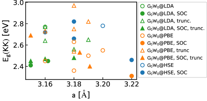
They are obtained with and without SOC (filled and open symbols, respectively), as well as with and without truncation of the Coulomb potential (triangles and circles, respectively), using LDA, PBE, and HSE as starting points (green, orange and blue, respectively). Supplementary Table 4 summarizes these data.
Fig. 2: Top view (left) and side view (middle) of the MoS2 slab geometry, determined by the in-plane lattice constant a and the distance between sulfur atoms, dSS. 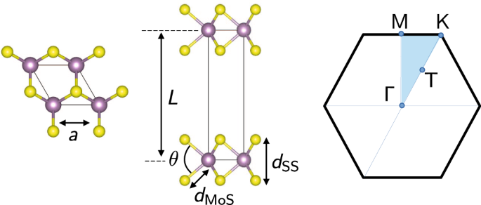
The Mo-S bond length dMoS and the S-Mo-S angle θ are shown as well. L is the unit-cell size along the out-of-plane direction z, including a vacuum layer. High-symmetry points and paths used in the band-structure plots (Fig. 4) are highlighted in the BZ (right panel).


In this manuscript, we address all these issues and provide a benchmark data set of density functional theory (DFT) and G0W0 calculations, taking monolayer MoS2 as a representative 2D material. Due to its unique properties, it can be considered the most important 2D material after graphene. MoS2 exhibits high electron mobility14,78; moderate SOC that can be exploited in spin- and valleytronics79,80,81,82,83,84,85; a direct fundamental band gap with intermediately strong exciton binding, which is suitable for (opto)electronic devices operating at room temperature14,29,31,38,78,86. For these reasons, there are many experimental and theoretical works in the literature that investigate MoS2, allowing for a better comparison with our results.
We employ the linearized augmented planewave + local orbital (in short LAPW+LO) method as implemented in the exciting code. LAPW+LO is known to achieve ultimate precision for solving the Kohn-Sham (KS) equations of DFT87 and high-level GW results88. Besides the local and semilocal DFT functionals LDA89 and PBE90,91 respectively, we include HSE0692,93,94 both for geometry optimization and as a starting point for G0W0. So far, HSE06 has not often been used for such calculations of MoS220,22,29,33, and to the best of our knowledge, neither a Coulomb truncation nor an adequate treatment of the singularity at q = 0 was applied. For brevity, hereafter, we will refer to HSE06 as HSE. In our G0W0 calculations, we truncate the Coulomb potential28,49,95, and apply a special analytical treatment for the q = 0 singularity24. Moreover, we investigate the role of SOC at all levels. We carefully evaluate the impact of all these elements and conclude what leads to the most reliable electronic structure of this important material. Besides a detailed analysis of energy gaps, we address effective masses and spin-orbit splittings.
Results
Ground-state geometries
The geometry of MoS2, depicted in Fig. 2, is determined by the in-plane lattice parameter a and the distance between sulfur atoms, dSS. In Table 1, we list these structural parameters as obtained with LDA, PBE, and HSE, and include the Mo-S bond length dMoS and the angle θ between Mo and S atoms as well. As expected, LDA underestimates the lattice spacing, PBE slightly overestimates it, and HSE shows the best performance with respect to experiment. All three exchange-correlation (xc) functionals underestimate the S-S bond length, PBE being closest to its measured counterpart. Comparison with computed literature data reveals good agreement.
Electronic structure
Table 2 summarizes the energy gaps obtained with different functionals for the different geometries. We consider here the direct gap at the K point (Eg(KK)) as well as the indirect gaps between Γ and K (Eg(ΓK)) and between K and T (Eg(KT)). For the definition of the T point, see Fig. 2. For each geometry and methodology, the bold font highlights the fundamental gap. For the calculations that include SOC, Fig. 3 displays the energy gaps given in Table 2 with respect to the lattice parameter. In the DFT calculations, regardless of the calculation method, Eg(KT) (squares) shows a weak dependence on the geometry. The fundamental gap obtained with LDA, PBE, and HSE, is always direct at K. In G0W0, the fundamental gap is Eg(KT) for the structures with smaller lattice parameter and Eg(KK) for larger lattice constants.

The values for KK, ΓK, and KT are represented as circles, triangles, and squares, respectively. Dotted (solid) lines stand for DFT (G0W0) results; all include SOC. Note that these values only indirectly reflect the S-S distance dSS.
As to be expected and also observed in ref. 38, for a fixed geometry, the energy gaps obtained by LDA and PBE are quite similar, with the largest difference being 0.02 eV. The two functionals also agree on the location of the valence-band maximum (VBM) and the conduction-band minimum (CBm). For both, the band gap is direct if SOC is included, and indirect otherwise for the PBE and HSE geometries. In contrast, HSE gives a direct gap, regardless of whether SOC is considered.
Also G0W0@LDA and G0W0@PBE are very close to each other, the largest difference being 0.04 eV. This can be attributed to the similarity between LDA and PBE when the same geometry is adopted. However, the similarity between G0W0@LDA and G0W0@PBE results is material dependent, as observed in other works96,97,98,99.
For a given geometry, the locations of the VBM and the CBm are independent of the starting point, with the only exception being the HSE geometry when SOC is included. When comparing the three geometries, we encounter three different scenarios. First, for the LDA geometry, the fundamental gap changes from a direct KS gap at K to an indirect QP gap (between K and T), independent of the starting point. Second, for the PBE and HSE geometries, when SOC is disregarded, the indirect gap ΓK obtained withII D LDA and PBE becomes direct and located at K upon applying G0W0. Third, for the HSE geometry, and SOC being included we observe an indirect band gap for G0W0@LDA while it is direct for PBE and HSE as starting points. This can be understood in terms of the small differences between the KK and KT gaps, ΔKT, which are 0.01 eV, 0.05 eV, and 0.15 eV for G0W0@LDA, G0W0@PBE and G0W0@HSE, respectively. Including SOC, splits the conduction band state at T (K) by ~0.07 eV (~3 meV), decreasing ΔKT by ~0.03 eV. This is enough to make ΔKT negative for G0W0@LDA, but not for G0W0@PBE, and G0W0@HSE. A more detailed discussion about ΔKT can be found in Section “Discussion of energy gaps: comparison with experiment”.
Figure 4 shows the band structures obtained for the HSE geometry including SOC. As expected, the differences between G0W0@HSE and HSE bands are less pronounced than those between G0W0@LDA (G0W0@PBE) and LDA (PBE) bands. For all three starting points, the G0W0 corrections are not uniform over all k-points, i.e., a simple scissors approximation is, strictly speaking, not applicable. We will explore this in a more quantitative fashion further below. The SOC splitting in the valence band is zero at the Γ point and increases toward the K point. The SOC effect on the conduction bands is much less pronounced. These observations are in agreement with other theoretical25,29,100,101,102,103 and experimental works86,104.

The parameters ΔKT and ΔΓK are discussed in Section “Discussion of energy gaps: comparison with experiment”.
The impact of the self-energy correction on the energy gaps, \(\Delta {{{{\rm{E}}}}}_{{{{\rm{g}}}}}={{{{{\rm{E}}}}}_{{{{\rm{g}}}}}}^{{G}_{0}{W}_{0}}-{{{{\rm{E}}}}}_{{{{\rm{g}}}}}^{{{{\rm{DFT}}}}}\), is shown in Fig. 5 for the case when SOC is included. Clearly, ΔEg is more significant for (semi)local DFT starting points than for HSE. Interestingly, for a given starting point, ΔEg hardly depends on the geometry. For LDA and PBE as the starting points, the ranges of ΔEg(KK), ΔEg(ΓK), and ΔEg(KT) are 0.84–0.90, 1.0–1.1, and 0.61–0.65 eV, respectively. The dependence is even weaker for G0W0@HSE with values of 0.64–0.66, 0.74–0.78, and 0.39–0.40 eV, respectively. Very similar results are observed when SOC is disregarded.

Left, middle, and right panels refer to ΔEg evaluated at the K point, between Γ and K, and between K and T, respectively.
Spin-orbit splittings and effective masses
In Table 3, we report for the HSE structure the spin-orbit splitting Δval (Δcond) at the K point for the highest occupied (lowest unoccupied) band. Effective electron (hole) masses me (mh) calculated at the K point along different directions are shown as well. We observe that neither the spin-orbit splittings nor the effective masses are very sensitive to the geometry (see Supplementary Table 11 for more details).
Δval exhibits a very narrow spread among all the methods employed here (DFT and G0W0), i.e., a range of 143–149 meV. These values are in excellent agreement with the experimental counterparts of Δval = 130–160 meV86,102,104,105,106,107,108. The value for the conduction band, Δcond, is 3 meV for LDA, PBE, G0W0@LDA, and G0W0@PBE; it is only slightly higher for HSE and G0W0@HSE, namely 4 meV. Again, there is excellent agreement with the measured value of Δcond = 4.3 ± 0.1 meV109.
The effective hole mass, mh, exhibits minor variations, not larger than 0.04m0, when going from KΓ to KM. This is in line with other calculations27,110. The measured value for freestanding MoS2 is mh = (0.43 ± 0.02)m0111 and, apart from LDA and PBE, all theoretical results show excellent agreement. The electron mass, me, is more isotropic than mh. For LDA, it differs by at most 0.02m0 between KΓ and KM. Our values are in line with other calculated results18,21,27,34,101,110,112. The measured counterpart of (0.67 ± 0.08)m0113 is significantly larger than the calculated value reported here and in other theoretical works18,21,27,34,101,110,112. As discussed in ref. 34, the difference could originate from the heavy doping of the measured sample, which may introduce metallic screening.
Discussion of energy gaps: comparison with experiment
The experimental band gap for free-standing MoS2, determined by photocurrent spectroscopy, is 2.5 eV86. In order to compare with experiment, it is important to account for the zero-point renormalization energy of 75 meV114. This means that the theoretical value computed without this correction should be 2.575 ≅ 2.6 eV to match its measured counterpart. For our discussion here, we consider the HSE and PBE geometries, which are closer to experiment than that obtained by LDA. For the following assessment, we refer to the values in Table 2. For the structure optimized with HSE, G0W0 performed on LDA, PBE, and HSE as starting points gives Eg(KK) of 2.52, 2.52, and 2.76 eV, respectively, i.e., G0W0@LDA and G0W0@PBE underestimate the measured value by about 0.08 eV, whereas G0W0@HSE overestimates it by 0.16 eV. However, even though G0W0@LDA agrees better with experiment than G0W0@HSE, it erroneously predicts an indirect band gap Eg(KT) which is 0.02 eV smaller than Eg(KK). G0W0@PBE shows the best agreement with experiment and also predicts the gap to be direct. Interestingly, considering the PBE geometry, as done in several works19,21,22,23,24,28,31,32,33,35,40,41,42,43,112, G0W0@HSE, giving a direct band gap of Eg(KK) = 2.68 eV, agrees best with experiment, the deviation being 0.08 eV only. With LDA and PBE as starting points, the calculated G0W0 band gap is direct, but 0.16 and 0.15 eV, respectively, below the experimental value.
Other relevant aspects of the band-structure concern relative energy differences, in particular ΔKT (introduced above) as well as the maximum energy at the Γ point wrt the VBM at the K point, ΔΓK = Eg(KK) − Eg(ΓK) (see Fig. 4). Experimentally, ΔKT is expected to be ≳ 60 meV101,113 and ΔΓK ≈ 140 meV101,115. Taking our calculations with SOC at the HSE geometry, (see Table 4), the G0W0@HSE value of 0.12 eV reproduces ΔKT best. On the other hand, HSE satisfies ΔΓK best with a value of 0.12 eV (0.02 eV smaller than in experiment), while the values obtained with the other methods differ from experiment by 0.09 eV (G0W0@HSE), −0.09 eV (LDA and PBE), 0.10 eV (G0W0@PBE), and 0.11 eV eV (G0W0@LDA), respectively. At the PBE geometry, G0W0@HSE and G0W0@PBE give the same value for ΔΓK. With an overestimation of 0.07 eV, it is closer to experiment than the value at the HSE geometry. Again, HSE is the only starting point for which G0W0 predicts ΔKT in agreement with experiment.
In summary, considering the band gap as well as the energy differences ΔKT and ΔΓK, we conclude that at the PBE geometry, G0W0@HSE including SOC shows the best overall agreement with experimental data. Also for the HSE structure, HSE is the best starting point, with results that are overall only slightly worse. Overall, G0W0@HSE at the HSE geometry can be considered more appropriate, since only one xc functional is needed for providing decent results for both, the geometry and the electronic properties and thus the most consistent picture. Also for other materials, HSE has been found to be a superior G0W0 starting point76,116,117,118 compared to LDA and PBE. For such materials with intermediate band gaps,71,72,119,120,121,122,123,124, this functional better justifies the perturbative self-energy correction68,73,116. Figure 5 confirms this for MoS2.
Discussion of energy gaps: comparison with theoretical works
By employing coupled-cluster calculations including singles and doubles125,126, Pulkin et al. obtained energy gaps of Eg(ΓK) = 2.93 eV and Eg(KK) = 3.00 eV with an error bar of ± 0.05 eV112 for the PBE geometry of ref. 103; SOC was not included. For our PBE geometry and also omitting SOC, the G0W0@HSE results are the ones closest to these values, with Eg(ΓK) differing by 0.04 eV and Eg(KK) by 0.24 eV.
For a fair comparison with other published G0W0 values with LDA and PBE as starting points, we restrict ourselves here to results obtained by using a Coulomb truncation in combination with either a special treatment of the q = 0 singularity or a nonuniform k-grid sampling, since these methods ensure well converged gaps. In ref. 24, disregarding SOC and adopting the PBE geometry (a = 3.184 Å, dSS = 3.127 Å), a direct band gap of 2.54 eV was reported for G0W0@PBE which is very close to ours (Eg(KK) = 2.52 eV), i.e., differing by only 0.02 eV. Including SOC and the thus slightly changed PBE geometry (a = 3.18 Å, dSS = 3.13 Å), a G0W0@LDA value of 2.48 eV was obtained in ref. 23; at basically the same geometry (differences in the order of 10−3 Å), our results of Eg(KK) = 2.44 eV is only 0.04 eV smaller.
For a lattice parameter of 3.15 Å, Rasmussen et al. calculated a G0W0@PBE band gap of 2.64 eV without SOC24. For the same lattice constant, but including SOC, Qiu et al. reported a G0W0@LDA band gap of38 of Eg(KK) = 2.59 eV with the plasmon-pole model and Eg(KK) = 2.45 eV with the contour deformation method. In our case, the structure optimized with HSE (a = 3.160 Å) is closest to a = 3.15 Å. For this structure, without including SOC, we compute a G0W0@PBE band gap of Eg(KK) = 2.60 eV, which agrees quite well with the one by ref. 24, differing by less than 0.04 eV. When we include SOC, we obtain Eg(KK) = 2.52 eV with G0W0@LDA, although at this geometry, we obtain an indirect gap that is 18 meV smaller than Eg(KK). This is in good agreement with ref. 38, with a difference of 0.07 meV only.
For the experimental geometry and neglecting SOC, ref. 28 reported values of Eg(KT) = 2.58 eV and Eg(KK) = 2.77 eV for G0W0@LDA. In our case, at the HSE geometry, we obtain Eg(KT) = 2.61 eV and Eg(KK) = 2.60 eV. As the HSE geometry is close to experiment, we may attribute the discrepancies mainly to the different underlying KS states. Indeed, at the LDA level, the energy gaps in ref. 28 are Eg(KK) = 1.77 eV and Eg(ΓK) = 1.83 eV28, while ours are Eg(KK) = 1.73 eV and Eg(ΓK) = 1.71 eV. The values for ΔEg, however, compare fairly well (ΔEg(KK) = 1.00 eV, ΔEg(KT) = 0.6–0.7 eV in ref. 28, compared to ΔEg(KK) = 0.87 eV, ΔEg(KT) = 0.63 eV in the present work).
When it comes to G0W0@HSE, there are only a few results for MoS2 in the literature, neither obtained with Coulomb truncation nor by any special treatment of the q = 0 singularity. For MoS2, these two aspects lead to opposite effects, competing with each other when converging band gaps with respect to the vacuum size and the number of k-points24: Neglecting them, band gaps increase when the vacuum layer is enlarged, whereas denser k-grids make them decrease. Hence, due to fortunate error cancellation, an insufficient vacuum length combined with a coarse k-grid may lead to G0W0 band gaps that agree well with those obtained in a highly converged situation24,29. In ref. 33, using the PBE geometry and taking SOC into account, a KK gap of 2.66 eV was reported. With 15 Å of vacuum, a 6 × 6 × 1 k-grid, and adopting the PBE geometry, in ref. 22, band gaps of 2.05 and 2.82 eV at the HSE and G0W0 levels, respectively, have been obtained. The HSE band gap agrees quite well with ours (2.04 eV), whereas our G0W0@HSE06 gap is 0.14 eV smaller. The band gap of 2.72 eV reported in ref. 29 is based on the experimental lattice parameter of 3.16 Å, a 12 × 12 × 1 k-points grid, and a vacuum layer of 17 Å, and includes SOC effects. The authors state to have chosen these settings to take advantage of error cancellation in the band gap29, and, surprisingly, our band gap of 2.76 eV obtained with G0W0@HSE at the HSE geometry (a = 3.160 Å) agrees quite well.
Closing remarks
We have employed the LAPW+LO method to provide a set of benchmark G0W0 calculations of the electronic structure of two-dimensional MoS2. We have addressed the impact of geometry, SOC, and DFT starting point on the energy gaps, spin-orbit splittings, and effective masses. We find that the self-energy corrections to the band gaps hardly depend on the adopted geometry. As could be expected, employing LDA and PBE as starting points does not make a significant difference when the same structure is used. The best agreement with experimental results is achieved by G0W0@HSE at either the HSE or PBE geometry, considering SOC. The spin-splittings obtained with all methods agree well with experimental results. This also holds true for the effective hole mass, using either HSE or G0W0 on top of any of the considered starting points (LDA, PBE, and HSE). In line with other theoretical works, we highlight the importance of a Coulomb truncation and an adequate treatment of the Coulomb singularity around q = 0 as being fundamental for high-quality calculations. Our findings are expected to be valid for other two-dimensional materials as well.
Methods
Linearized augmented planewave + local orbital methods
The full-potential all-electron code exciting127 implements the family of LAPW+LO methods. In this framework, the unit cell is divided into non-overlapping muffin-tin (MT) spheres, centered at the atomic positions, and the interstitial region in between the spheres. exciting treats all electrons in a calculation by distinguishing between core and valence/semi-core states. For core electrons, assumed to be confined inside the respective MT sphere, the KS potential is employed to solve the Dirac equation which captures relativistic effects including SOC. The KS wavefunctions \(\left\vert {\Psi }_{n{{{\bf{k}}}}}\right\rangle\) for valence and semicore states, characterized by band index n and wavevector k, are expanded in terms of augmented planewaves, \(\left\vert {\phi }_{{{{\bf{G}}}}+{{{\bf{k}}}}}\right\rangle\), and local orbitals, \(\vert {\phi }_{\gamma }\rangle\), as
\(\left\vert {\phi }_{{{{\bf{G}}}}+{{{\bf{k}}}}}\right\rangle\) are constructed by augmenting each planewave with reciprocal lattice vector G, living in the interstitial region, by a linear combination of atomic-like functions inside the MT spheres. In contrast, the LOs \(\vert {\phi }_{\gamma }\rangle\) are non-zero only inside a specific MT sphere. They are used for reducing the linearization error127,128, for the description of semicore states, as well as for improving the basis set for unoccupied states87,88. The quality of the basis set can be systematically improved by increasing the number of augmented planewaves (controlled in exciting by the dimensionless parameter rgkmax) and by introducing more LOs87,127. With all these features, exciting can be regarded as a reference code not only for solving the KS equation129, where it is capable of reaching micro-Hartree precision87, but also for G0W0 calculations88.
G 0 W 0 approximation
In the G0W0 approximation, one takes a set of KS eigenvalues {εnk} and eigenfunctions {Ψnk} as a reference, and evaluates first-order quasi-particle (QP) corrections to the KS eigenvalues in first-order perturbation theory as
where Znk is the renormalization factor, Vxc is the xc potential, and Σ is the self-energy. The latter is given as the convolution
with G being the single-particle Green function and W the screened Coulomb potential.
In this non-selfconsistent method, the quality of the QP eigenvalues may depend critically on the starting point. In many cases, LDA and PBE have been proven to be good starting points for G0W0, leading to QP energies that agree well with experiments73,130,131. However, e.g., for materials containing d electrons, such as Mo, hybrid functionals, like HSE, usually provide an improved reference for QP corrections compared to semilocal functionals71,72,119,120,121,122,123,124. Here, we evaluate the quality of each of these three as a starting point.
Coulomb truncation
In calculations with periodic boundary conditions, for treating 2D systems, a sufficient amount of vacuum is required to avoid spurious interaction between the replica along the out-of-plane direction. Local and semilocal density functionals have a (nonphysical) asymptotic decay much faster than 1/r, facilitating convergence of unoccupied states –and thus KS gaps– with respect to the vacuum size. In G0W0, the 1/r decay of the self-energy complicates this task. Specifically for MoS2, even a vacuum layer with 60 Å thickness turned out not being sufficient to obtain a fully converged band gap28,49. Truncating the Coulomb potential along the out-of-plane direction z, however, leads to well-converged G0W0 band gaps with a considerably smaller vacuum size28,49.
Here, we truncate the Coulomb potential with a step function along z. Setting the cutoff length to L/2, where L is the size of the supercell along z (Fig. 2), the truncated Coulomb potential can be written in a planewave basis as95:
where Q = q + G, and q is a vector in the first Brillouin zone (BZ).
Treatment of the q = 0 singularity
On the down-side, truncating the Coulomb interaction slows down the convergence in terms of k-points because of the non-smooth behavior of the dielectric function around the singularity at q = 023,24,41. To bypass this problem, we follow an analytical treatment of Wc, the correlation part of W, close to the singularity as proposed in ref. 24. Without this treatment, the correlation part of the self-energy Σc(ω) can be written as132
where \({\tilde{\epsilon }}_{n{{{\bf{k}}}}}={\epsilon }_{n{{{\bf{k}}}}}+{{{\rm{i}}}}\,\eta \,{{{\rm{sign}}}}({E}_{{{{\rm{F}}}}}-{\epsilon }_{n{{{\bf{k}}}}})\) and EF the Fermi energy. \({M}_{nm}^{i}({{{\bf{k}}}},{{{\bf{q}}}})\) are the expansion coefficients of the mixed-product basis, an auxiliary basis to represent products of KS wavefunctions. Like LAPWs and LOs, they have distinct characteristics in the MT spheres and interstitial region132,133. To treat the q = 0 case separately, the corresponding term in Eq. (5) is replaced by
where Ω0 is a small region around q = 0. Analytical expressions for \({W}_{ij}^{{{{\rm{c}}}}}({{{\bf{q}}}},{\omega }^{{\prime} })\) in the limit q → 024 are then employed to calculate the integral in Eq. (6).
Spin-orbit coupling
In this study, SOC is treated via the second-variational (SV) scheme134. In LDA and PBE calculations, the conventional SV approach is utilized127,135,136,137: First, the scalar-relativistic problem, i.e., omitting SOC, is solved. A subset of the resulting eigenvectors is then used as basis set for addressing the full problem. The number of eigenvectors is a convergence parameter. In this work, the SOC term is evaluated with the zero-order regular approximation (ZORA)138,139.
A ground-state calculation with HSE is performed via a nested loop140: In the outer loop, the nonlocal exchange is computed for a subset of KS wavefunctions, using a mixed-product basis. The inner loop solves the generalized KS equations self-consistently, where only the local part of the effective potential is updated in each step. Within this inner loop, the SV scheme is applied self-consistently to incorporate SOC. The corresponding term, evaluated within the ZORA, is based on PBE, which is justified by the minimal contribution due to the gradient of the nonlocal potential141,142,143.
G0W0 calculations with SOC are performed in two steps on top of ground-state calculations that include SOC. First, the QP energies are computed as explained in Section “G0W0 approximation”, using the scalar-relativistic KS eigenvalues and eigenvectors. In the second step, the obtained QP energies are used, together with the SV KS eigenvectors, to evaluate SOC through the diagonalization of the SV Hamiltonian. This approach is sufficient in the case of MoS2 since SOC does not cause band inversion133,143.
Computational details
In our calculations, we employ the all-electron full-potential code exciting127. The only exception is for obtaining the HSE equilibrium geometry, where FHI-aims144,145 is used, since so far exciting lacks geometry relaxation with hybrid functionals. Even though exciting and FHI-aims implement very different basis sets to expand the KS wavefunctions, the two codes have been shown to be among those with the best mutual agreement129. Moreover, a comparison of energy gaps and geometry relaxations for MoS2 confirms this finding (see Supplementary Information - Section I).
In all calculations, the unit-cell size L along the out-of-plane direction (Fig. 2) is set to 30 bohr. Different flavors of xc functionals are applied, namely LDA, PBE, and HSE. In the latter, we use the typical parameters94, i.e., a mixing factor of α = 0.25 and a screening range of ω = 0.11 bohr−1. To determine the respective equilibrium geometries, we relax the atomic positions until the total force on each ion is smaller than 10 μHa bohr−1. For these geometries, the electronic structure is calculated with all three functionals, with and without SOC, giving rise to a set of 18 calculations. These calculations are followed by G0W0 calculations, taking the respective DFT solutions as starting points.
The dimensionless parameter rgkmax that controls the exciting basis-set size is set to 8. In the LDA and PBE calculations, we use a 30 × 30 × 1 k-grid. In HSE and G0W0 calculations, we employ 400 empty states and an 18 × 18 × 1 k-grid. In G0W0, the correlation part of the self-energy is evaluated with 32 frequency points along the imaginary axis, and then analytic continuation to the real axis is carried out by means of Pade’s approximant. For the bare Coulomb potential, we use a 2D cutoff95 combined with a special treatment of the q = 0 singularity as described in Section “Treatment of the q = 0 singularity”. Furthermore, we carefully determine the minimal set of LOs, sufficient to converge at least the lowest 400 KS states. This is achieved with 2 and 6 LOs for sulfur s and p states, respectively, as well as 3, 6, and 10 LOs for molybdenum s, p, and d states, respectively. Overall, we estimate a numerical precision of 50–100 meV in the energy gaps obtained with our G0W0 calculations. To determine effective masses, we use parabolic fits within a range of 0.05 Å−1 around the VBM and the CBm at the K point of the BZ. Depending on the respective case, K can host either global or local extrema.
Data availability
All input and output files are available at NOMAD146,147 under https://doi.org/10.17172/NOMAD/2023.09.16-1.
References
Geim, A. K. & Novoselov, K. S. The rise of graphene. Nat. Mater. 6, 183–191 (2007).
Shanmugam, V. et al. A review of the synthesis, properties, and applications of 2d materials. Part. Part. Syst. Char. 39, 2200031 (2022).
Kumbhakar, P. et al. Prospective applications of two-dimensional materials beyond laboratory frontiers: a review. iScience 26, 106671 (2023).
Mir, S. H., Yadav, V. K. & Singh, J. K. Recent advances in the carrier mobility of two-dimensional materials: a theoretical perspective. ACS Omega 5, 14203–14211 (2020).
Zeng, M., Xiao, Y., Liu, J., Yang, K. & Fu, L. Exploring two-dimensional materials toward the next-generation circuits: from monomer design to assembly control. Chem. Rev. 118, 6236–6296 (2018).
Zhang, H. Introduction: 2d materials chemistry. Chem. Rev. 118, 6089–6090 (2018).
Chaves, A. et al. Bandgap engineering of two-dimensional semiconductor materials. npj 2D Mater. Appl. 4, 29 (2020).
Guinea, F., Katsnelson, M. I. & Wehling, T. O. Two-dimensional materials: electronic structure and many-body effects. Ann. Phys. 526, A81–A82 (2014).
Xiao, J., Zhao, M., Wang, Y. & Zhang, X. Excitons in atomically thin 2D semiconductors and their applications. Nanophotonics 6, 1309–1328 (2017).
Mueller, T. & Malic, E. Exciton physics and device application of two-dimensional transition metal dichalcogenide semiconductors. npj 2D Mater. Appl. 2, 29 (2018).
Thygesen, K. S. Calculating excitons, plasmons, and quasiparticles in 2D materials and van der Waals heterostructures. 2D Mater. 4, 022004 (2017).
Mir, S. H. Exploring the electronic, charge transport and lattice dynamic properties of two-dimensional phosphorene. Phys. B: Condens. Matter 572, 88–93 (2019).
Bolotin, K. I. et al. Ultrahigh electron mobility in suspended graphene. Solid State Commun. 146, 351–355 (2008).
Radisavljevic, B., Radenovic, A., Brivio, J., Giacometti, V. & Kis, A. Single-layer MoS2 transistors. Nat. Nanotechnol. 6, 147–150 (2011).
Liu, Y. et al. Van der waals heterostructures and devices. Nat. Rev. Mater. 1, 1–17 (2016).
Jariwala, D., Sangwan, V. K., Lauhon, L. J., Marks, T. J. & Hersam, M. C. Emerging device applications for semiconducting two-dimensional transition metal dichalcogenides. ACS Nano 8, 1102–1120 (2014).
Wang, Q. H., Kalantar-Zadeh, K., Kis, A., Coleman, J. N. & Strano, M. S. Electronics and optoelectronics of two-dimensional transition metal dichalcogenides. Nat. Nanotechnol. 7, 699–712 (2012).
Molina-Sánchez, A., Hummer, K. & Wirtz, L. Vibrational and optical properties of MoS2: from monolayer to bulk. Surf. Sci. Rep. 70, 554–586 (2015).
Conley, H. J. et al. Bandgap Engineering Of Strained Monolayer And Bilayer MoS2. Nano Lett. 13, 3626–3630 (2013).
Ataca, C. & Ciraci, S. Functionalization of single-layer MoS2 honeycomb structures. J. Phys. Chem. C 115, 13303–13311 (2011).
Shi, H., Pan, H., Zhang, Y.-W. & Yakobson, B. I. Quasiparticle band structures and optical properties of strained monolayer MoS2 and WS2. Phys. Rev. B 87, 155304 (2013).
Ramasubramaniam, A. Large excitonic effects in monolayers of molybdenum and tungsten dichalcogenides. Phys. Rev. B 86, 115409 (2012).
Rasmussen, F. A. & Thygesen, K. S. Computational 2D materials database: electronic structure of transition-metal dichalcogenides and oxides. J. Phys. Chem. C 119, 13169–13183 (2015).
Rasmussen, F. A., Schmidt, P. S., Winther, K. T. & Thygesen, K. S. Efficient many-body calculations for two-dimensional materials using exact limits for the screened potential: Band gaps of MoS2, h-BN, and phosphorene. Phys. Rev. B 94, 155406 (2016).
Molina-Sánchez, A., Sangalli, D., Hummer, K., Marini, A. & Wirtz, L. Effect of spin-orbit interaction on the optical spectra of single-layer, double-layer, and bulk MoS2. Phys. Rev. B 88, 045412 (2013).
Qiu, D. Y., Jornada, F. H. D. & Louie, S. G. Optical spectrum of MoS2: many-body effects and diversity of exciton states. Phys. Rev. Lett. 111, 216805 (2013).
Cheiwchanchamnangij, T. & Lambrecht, W. R. L. Quasiparticle band structure calculation of monolayer, bilayer, and bulk MoS2. Phys. Rev. B 85, 205302 (2012).
Hüser, F., Olsen, T. & Thygesen, K. S. How dielectric screening in two-dimensional crystals affects the convergence of excited-state calculations: monolayer MoS2. Phys. Rev. B 88, 245309 (2013).
Echeverry, J. P., Urbaszek, B., Amand, T., Marie, X. & Gerber, I. C. Splitting between bright and dark excitons in transition metal dichalcogenide monolayers. Phys. Rev. B 93, 121107 (2016).
Schmidt, P. S., Patrick, C. E. & Thygesen, K. S. Simple vertex correction improves GW band energies of bulk and two-dimensional crystals. Phys. Rev. B 96, 205206 (2017).
Komsa, H.-P. & Krasheninnikov, A. V. Effects of confinement and environment on the electronic structure and exciton binding energy of MoS2 from first principles. Phys. Rev. B 86, 241201 (2012).
Liang, Y., Huang, S., Soklaski, R. & Yang, L. Quasiparticle band-edge energy and band offsets of monolayer of molybdenum and tungsten chalcogenides. Appl. Phys. Lett. 103, 042106 (2013).
Jiang, X. et al. Real-time GW-BSE investigations on spin-valley exciton dynamics in monolayer transition metal dichalcogenide. Sci. Adv. 7, eabf3759 (2021).
Zibouche, N., Schlipf, M. & Giustino, F. GW band structure of monolayer MoS2 using the SternheimerGW method and effect of dielectric environment. Phys. Rev. B 103, 125401 (2021).
Soklaski, R. et al. Temperature effect on optical spectra of monolayer molybdenum disulfide. Appl. Phys. Lett. 104, 193110 (2014).
Xia, W. et al. Combined subsampling and analytical integration for efficient large-scale GW calculations for 2D systems. npj Comput. Mater. 6, 118 (2020).
Gao, W., Xia, W., Gao, X. & Zhang, P. Speeding up GW calculations to meet the challenge of large scale quasiparticle predictions. Sci. Rep. 6, 36849 (2016).
Qiu, D. Y., Jornada, F. H. D. & Louie, S. G. Screening and many-body effects in two-dimensional crystals: Monolayer MoS2. Phys. Rev. B 93, 235435 (2016).
Gillen, R. & Maultzsch, J. Light-matter interactions in two-dimensional transition metal dichalcogenides: dominant excitonic transitions in mono-and few-layer MoX2 and band nesting. IEEE J. Quantum Electron. 23, 219–230 (2016).
Zhuang, H. L. & Hennig, R. G. Computational search for single-layer transition-metal dichalcogenide photocatalysts. J. Phys. Chem. C 117, 20440–20445 (2013).
Haastrup, S. et al. The computational 2D materials database: high-throughput modeling and discovery of atomically thin crystals. 2D Mater. 5, 042002 (2018).
Gjerding, M. N. et al. Recent progress of the computational 2d materials database (c2db). 2D Mater. 8, 044002 (2021).
Kim, H.-g & Choi, H. J. Thickness dependence of work function, ionization energy, and electron affinity of Mo and W dichalcogenides from DFT and GW calculations. Phys. Rev. B 103, 085404 (2021).
Smart, T. J., Wu, F., Govoni, M. & Ping, Y. Fundamental principles for calculating charged defect ionization energies in ultrathin two-dimensional materials. Phys. Rev. Mater. 2, 124002 (2018).
Horzum, S. et al. Phonon softening and direct to indirect band gap crossover in strained single-layer MoSe2. Phys. Rev. B 87, 125415 (2013).
Lee, J., Huang, J., Sumpter, B. G. & Yoon, M. Strain-engineered optoelectronic properties of 2d transition metal dichalcogenide lateral heterostructures. 2D Mater. 4, 021016 (2017).
Elliott, J. D. et al. Surface susceptibility and conductivity of MoS2 and WSe2 monolayers: a first-principles and ellipsometry characterization. Phys. Rev. B 101, 045414 (2020).
Kirchhoff, A., Deilmann, T., Krüger, P. & Rohlfing, M. Electronic and optical properties of a hexagonal boron nitride monolayer in its pristine form and with point defects from first principles. Phys. Rev. B 106, 045118 (2022).
Hüser, F., Olsen, T. & Thygesen, K. S. Quasiparticle GW calculations for solids, molecules, and two-dimensional materials. Phys. Rev. B 87, 235132 (2013).
Ferreira, F., Chaves, A., Peres, N. & Ribeiro, R. Excitons in hexagonal boron nitride single-layer: a new platform for polaritonics in the ultraviolet. J. Opt. Soc. Am. B 36, 674–683 (2019).
Attaccalite, C., Bockstedte, M., Marini, A., Rubio, A. & Wirtz, L. Coupling of excitons and defect states in boron-nitride nanostructures. Phys. Rev. B 83, 144115 (2011).
Galvani, T. et al. Excitons in boron nitride single layer. Phys. Rev. B 94, 125303 (2016).
Wu, F., Galatas, A., Sundararaman, R., Rocca, D. & Ping, Y. First-principles engineering of charged defects for two-dimensional quantum technologies. Phys. Rev. Mater. 1, 071001 (2017).
Blase, X., Rubio, A., Louie, S. G. & Cohen, M. L. Quasiparticle band structure of bulk hexagonal boron nitride and related systems. Phys. Rev. B 51, 6868–6875 (1995).
Wang, D. & Sundararaman, R. Layer dependence of defect charge transition levels in two-dimensional materials. Phys. Rev. B 101, 054103 (2020).
Mengle, K. A. & Kioupakis, E. Impact of the stacking sequence on the bandgap and luminescence properties of bulk, bilayer, and monolayer hexagonal boron nitride. APL Mater. 7, 021106 (2019).
Fu, Q., Nabok, D. & Draxl, C. Energy-level alignment at the interface of graphene fluoride and boron nitride monolayers: an investigation by many-body perturbation theory. J. Phys. Chem. C 120, 11671–11678 (2016).
Berseneva, N., Gulans, A., Krasheninnikov, A. V. & Nieminen, R. M. Electronic structure of boron nitride sheets doped with carbon from first-principles calculations. Phys. Rev. B 87, 035404 (2013).
Cudazzo, P. et al. Exciton band structure in two-dimensional materials. Phys. Rev. Lett. 116, 066803 (2016).
Ferreira, F. & Ribeiro, R. M. Improvements in the GW and Bethe-Salpeter-equation calculations on phosphorene. Phys. Rev. B 96, 115431 (2017).
Marsoner Steinkasserer, L. E., Suhr, S. & Paulus, B. Band-gap control in phosphorene/BN structures from first-principles calculations. Phys. Rev. B 94, 125444 (2016).
Rudenko, A. N. & Katsnelson, M. I. Quasiparticle band structure and tight-binding model for single- and bilayer black phosphorus. Phys. Rev. B 89, 201408 (2014).
Tran, V., Soklaski, R., Liang, Y. & Yang, L. Layer-controlled band gap and anisotropic excitons in few-layer black phosphorus. Phys. Rev. B 89, 235319 (2014).
Çakır, D., Sahin, H. & Peeters, FmcM. Tuning of the electronic and optical properties of single-layer black phosphorus by strain. Phys. Rev. B 90, 205421 (2014).
Tran, V., Fei, R. & Yang, L. Quasiparticle energies, excitons, and optical spectra of few-layer black phosphorus. 2D Mater. 2, 044014 (2015).
Pisarra, M., Díaz, C. & Martín, F. Theoretical study of structural and electronic properties of 2H-phase transition metal dichalcogenides. Phys. Rev. B 103, 195416 (2021).
Ortenzi, L., Pietronero, L. & Cappelluti, E. Zero-point motion and direct-indirect band-gap crossover in layered transition-metal dichalcogenides. Phys. Rev. B 98, 195313 (2018).
Bechstedt, F. Many-body approach to electronic excitations (Springer, 2016).
Onida, G., Reining, L. & Rubio, A. Electronic excitations: density-functional versus many-body Green’s-function approaches. Rev. Mod. Phys. 74, 601–659 (2002).
Li, X.-Z., Gómez-Abal, R., Jiang, H., Ambrosch-Draxl, C. & Scheffler, M. Impact of widely used approximations to the G0W0 method: an all-electron perspective. N. J. Phys. 14, 023006 (2012).
Körzdörfer, T. & Marom, N. Strategy for finding a reliable starting point for G0W0 demonstrated for molecules. Phys. Rev. B 86, 041110 (2012).
Chen, W. & Pasquarello, A. Band-edge positions in GW: effects of starting point and self-consistency. Phys. Rev. B 90, 165133 (2014).
Pela, R. R., Werner, U., Nabok, D. & Draxl, C. Probing the LDA-1/2 method as a starting point for G0W0 calculations. Phys. Rev. B 94, 235141 (2016).
McKeon, C. A., Hamed, S. M., Bruneval, F. & Neaton, J. B. An optimally tuned range-separated hybrid starting point for ab initio GW plus Bethe-Salpeter equation calculations of molecules. J. Chem. Phys. 157, 074103 (2022).
Knight, J. W. et al. Accurate ionization potentials and electron affinities of acceptor molecules III: a benchmark of GW methods. J. Chem. Theory Comput. 12, 615–626 (2016).
Gant, S. E. et al. Optimally tuned starting point for single-shot GW calculations of solids. Phys. Rev. Mater. 6, 053802 (2022).
Wang, L., Kutana, A. & Yakobson, B. I. Many-body and spin-orbit effects on direct-indirect band gap transition of strained monolayer MoS2 and WS2. Ann. Phys. 526, L7–L12 (2014).
Lembke, D. & Kis, A. Breakdown of high-performance monolayer MoS2 transistors. ACS Nano 6, 10070–10075 (2012).
Xiao, D., Liu, G.-B., Feng, W., Xu, X. & Yao, W. Coupled spin and valley physics in monolayers of MoS2 and other Group-VI Dichalcogenides. Phys. Rev. Lett. 108, 196802 (2012).
Cao, T. et al. Valley-selective circular dichroism of monolayer molybdenum disulphide. Nat. Commun. 3, 887 (2012).
Zeng, H., Dai, J., Yao, W., Xiao, D. & Cui, X. Valley polarization in MoS2 monolayers by optical pumping. Nat. Nanotechnol. 7, 490–493 (2012).
Yang, L. et al. Long-lived nanosecond spin relaxation and spin coherence of electrons in monolayer MoS2 and WS2. Nat. Phys. 11, 830–834 (2015).
Berghäuser, G. et al. Inverted valley polarization in optically excited transition metal dichalcogenides. Nat. Commun. 9, 971 (2018).
Caruso, F., Schebek, M., Pan, Y., Vona, C. & Draxl, C. Chirality of valley excitons in monolayer transition-metal dichalcogenides. J. Phys. Chem. Lett. 13, 5894–5899 (2022).
Ji, S. et al. Anomalous valley Hall effect induced by mirror symmetry breaking in transition metal dichalcogenides. Phys. Rev. B 107, 174434 (2023).
Klots, A. R. et al. Probing excitonic states in suspended two-dimensional semiconductors by photocurrent spectroscopy. Sci. Rep. 4, 6608 (2014).
Gulans, A., Kozhevnikov, A. & Draxl, C. Microhartree precision in density functional theory calculations. Phys. Rev. B 97, 161105 (2018).
Nabok, D., Gulans, A. & Draxl, C. Accurate all-electron G0W0 quasiparticle energies employing the full-potential augmented planewave method. Phys. Rev. B 94, 035118 (2016).
Perdew, J. P. & Wang, Y. Accurate and simple analytic representation of the electron-gas correlation energy. Phys. Rev. B 45, 13244–13249 (1992).
Perdew, J. P., Burke, K. & Ernzerhof, M. Generalized gradient approximation made simple. Phys. Rev. Lett. 77, 3865–3868 (1996).
Perdew, J. P., Burke, K. & Ernzerhof, M. Generalized gradient approximation made simple.Phys. Rev. Lett. 78, 1396–1396 (1997).
Heyd, J., Scuseria, G. E. & Ernzerhof, M. Hybrid functionals based on a screened Coulomb potential. J. Chem. Phys. 118, 8207–8215 (2003).
Heyd, J., Scuseria, G. E. & Ernzerhof, M. Erratum: “Hybrid functionals based on a screened Coulomb potential” [J. Chem. Phys. 118, 8207 (2003)]. J. Chem. Phys. 124, 219906 (2006).
Krukau, A. V., Vydrov, O. A., Izmaylov, A. F. & Scuseria, G. E. Influence of the exchange screening parameter on the performance of screened hybrid functionals. J. Chem. Phys. 125, 224106 (2006).
Ismail-Beigi, S. Truncation of periodic image interactions for confined systems. Phys. Rev. B 73, 233103 (2006).
Mansouri, M., Koval, P., Sharifzadeh, S. & Sánchez-Portal, D. Molecular doping in the organic semiconductor diindenoperylene: insights from many-body perturbation theory. J. Phys. Chem. C 127, 16668–16678 (2023).
Sun, J. & Ullrich, C. A. Optical properties of CsCu2X3 (X = Cl, Br, and I): a comparative study between hybrid time-dependent density-functional theory and the Bethe-Salpeter equation. Phys. Rev. Mater. 4, 095402 (2020).
Laflamme Janssen, J., Rousseau, B. & Côté, M. Efficient dielectric matrix calculations using the lanczos algorithm for fast many-body G0W0 implementations. Phys. Rev. B 91, 125120 (2015).
Klimeš, J., Kaltak, M. & Kresse, G. Predictive GW calculations using plane waves and pseudopotentials. Phys. Rev. B 90, 075125 (2014).
Salehi, S. & Saffarzadeh, A. Optoelectronic properties of defective MoS2 and WS2 monolayers. J. Phys. Chem. Solids 121, 172–176 (2018).
Kormányos, A. et al. k. p theory for two-dimensional transition metal dichalcogenide semiconductors. 2D Mater. 2, 022001 (2015).
Dou, X., Ding, K., Jiang, D., Fan, X. & Sun, B. Probing spin-orbit coupling and interlayer coupling in atomically thin molybdenum disulfide using hydrostatic pressure. ACS Nano 10, 1619–1624 (2016).
Zhu, Z. Y., Cheng, Y. C. & Schwingenschlögl, U. Giant spin-orbit-induced spin splitting in two-dimensional transition-metal dichalcogenide semiconductors. Phys. Rev. B 84, 153402 (2011).
Miwa, J. A. et al. Electronic structure of epitaxial single-layer MoS2. Phys. Rev. Lett. 114, 046802 (2014).
Zhang, Y. et al. On valence-band splitting in layered MoS2. ACS Nano 9, 8514–8519 (2015).
Splendiani, A. et al. Emerging photoluminescence in monolayer MoS2. Nano Lett. 10, 1271–1275 (2010).
Li, W. et al. Broadband optical properties of large-area monolayer CVD molybdenum disulfide. Phys. Rev. B 90, 195434 (2014).
Shen, C.-C., Hsu, Y.-T., Li, L.-J. & Liu, H.-L. Charge dynamics and electronic structures of monolayer MoS2 Films grown by chemical vapor deposition. Appl. Phys. Express 6, 125801 (2013).
Schmidt, H. et al. Quantum transport and observation of Dyakonov-Perel spin-orbit scattering in monolayer MoS2. Phys. Rev. Lett. 116, 046803 (2015).
Peelaers, H. & Walle, C. G. Vd Effects of strain on band structure and effective masses in MoS2. Phys. Rev. B 86, 241401 (2012).
Jin, W. et al. Substrate interactions with suspended and supported monolayer MoS 2: angle-resolved photoemission spectroscopy. Phys. Rev. B 91, 121409 (2015).
Pulkin, A. & Chan, G. K.-L. First-principles coupled cluster theory of the electronic spectrum of transition metal dichalcogenides. Phys. Rev. B 101, 241113 (2020).
Eknapakul, T. et al. Electronic structure of a Quasi-Freestanding MoS2 monolayer. Nano Lett. 14, 1312–1316 (2014).
Molina-Sánchez, A., Palummo, M., Marini, A. & Wirtz, L. Temperature-dependent excitonic effects in the optical properties of single-layer MoS2. Phys. Rev. B 93, 155435 (2016).
Jin, W. et al. Direct measurement of the thickness-dependent electronic band structure of MoS2 using angle-resolved photoemission spectroscopy. Phys. Rev. Lett. 111, 106801 (2013).
Fuchs, F., Furthmüller, J., Bechstedt, F., Shishkin, M. & Kresse, G. Quasiparticle band structure based on a generalized Kohn-Sham scheme. Phys. Rev. B 76, 115109 (2007).
Yadav, S. & Ramprasad, R. Strain-assisted bandgap modulation in Zn based II-VI semiconductors. Appl. Phys. Lett. 100, 241903 (2012).
Camarasa-Gómez, M., Ramasubramaniam, A., Neaton, J. B. & Kronik, L. Transferable screened range-separated hybrid functionals for electronic and optical properties of van der waals materials. Phys. Rev. Mater. 7, 104001 (2023).
Leppert, L., Rangel, T. & Neaton, J. B. Towards predictive band gaps for halide perovskites: Lessons from one-shot and eigenvalue self-consistent GW. Phys. Rev. Mater. 3, 103803 (2019).
Rinke, P., Qteish, A., Neugebauer, J., Freysoldt, C. & Scheffler, M. Combining GW calculations with exact-exchange density-functional theory: an analysis of valence-band photoemission for compound semiconductors. New J. Phys. 7, 126 (2005).
Atalla, V., Yoon, M., Caruso, F., Rinke, P. & Scheffler, M. Hybrid density functional theory meets quasiparticle calculations: a consistent electronic structure approach. Phys. Rev. B 88, 165122 (2013).
Bruneval, F. & Marques, M. A. Benchmarking the starting points of the GW approximation for molecules. J. Chem. Theory Comput. 9, 324–329 (2013).
Marom, N. et al. Benchmark of GW methods for azabenzenes. Phys. Rev. B 86, 245127 (2012).
Ren, X., Rinke, P. & Scheffler, M. Exploring the random phase approximation: application to CO adsorbed on Cu(111). Phys. Rev. B 80, 045402 (2009).
Cársky, P., Paldus, J. & Pittner, J. Recent progress in coupled cluster methods: theory and applications (Springer Science & Business Media, 2010).
Helgaker, T., Klopper, W. & Tew, D. P. Quantitative quantum chemistry. Mol. Phys. 106, 2107–2143 (2008).
Gulans, A. et al. exciting: a full-potential all-electron package implementing density-functional theory and many-body perturbation theory. J. Phys. Condens. Matter. 26, 363202 (2014).
Sjöstedt, E., Nordström, L. & Singh, D. An alternative way of linearizing the augmented plane-wave method. Solid State Commun. 114, 15–20 (2000).
Lejaeghere, K. et al. Reproducibility in density functional theory calculations of solids. Science 351, aad3000 (2016).
Aryasetiawan, F. & Gunnarsson, O. The GW method. Rep. Prog. Phys. 61, 237 (1998).
Kotani, T., van Schilfgaarde, M. & Faleev, S. V. Quasiparticle self-consistent GW method: a basis for the independent-particle approximation. Phys. Rev. B 76, 165106 (2007).
Jiang, H. et al. FHI-gap: a GW code based on the all-electron augmented plane wave method. Comput. Phys. Commun. 184, 348–366 (2013).
Aguilera, I., Friedrich, C. & Blügel, S. Spin-orbit coupling in quasiparticle studies of topological insulators. Phys. Rev. B 88, 165136 (2013).
Singh, D. J. Planes Waves, Pseudopotentials and the LAPW Method (Springer New York, NY, 1994).
MacDonald, A., Picket, W. & Koelling, D. A linearised relativistic augmented-plane-wave method utilising approximate pure spin basis functions. J. Phys. C Solid State Phys. 13, 2675 (1980).
Li, C., Freeman, A. J., Jansen, H. & Fu, C. Magnetic anisotropy in low-dimensional ferromagnetic systems: Fe monolayers on Ag (001), Au (001), and Pd (001) substrates. Phys. Rev. B 42, 5433 (1990).
Vona, C., Lubeck, S., Kleine, H., Gulans, A. & Draxl, C. Accurate and efficient treatment of spin-orbit coupling via second variation employing local orbitals. Phys. Rev. B 108, 235161 (2023).
Lenthe, E. V., Baerends, E. J. & Snijders, J. G. Relativistic regular two-component Hamiltonians. J. Chem. Phys. 99, 4597–4610 (1993).
van Lenthe, E., Baerends, E. J. & Snijders, J. G. Relativistic total energy using regular approximations. J. Chem. Phys. 101, 9783–9792 (1994).
Betzinger, M., Friedrich, C. & Blügel, S. Hybrid functionals within the all-electron FLAPW method: implementation and applications of PBE0. Phys. Rev. B 81, 195117 (2010).
Huhn, W. P. & Blum, V. One-hundred-three compound band-structure benchmark of post-self-consistent spin-orbit coupling treatments in density functional theory. Phys. Rev. Mater. 1, 033803 (2017).
Wang, M., Liu, G.-B., Guo, H. & Yao, Y. An efficient method for hybrid density functional calculation with spin-orbit coupling. Comput. Phys. Commun. 224, 90–97 (2018).
Vona, C., Nabok, D. & Draxl, C. Electronic structure of (Organic-)Inorganic metal halide perovskites: the dilemma of choosing the right functional. Adv. Theory Simul. 5, 2100496 (2022).
Blum, V. et al. Ab initio molecular simulations with numeric atom-centered orbitals. Comput. Phys. Commun. 180, 2175–2196 (2009).
Ren, X. et al. Resolution-of-identity approach to Hartree-Fock, hybrid density functionals, RPA, MP2 and GW with numeric atom-centered orbital basis functions. New J. Phys. 14, 053020 (2012).
Draxl, C. & Scheffler, M. The nomad laboratory: from data sharing to artificial intelligence. J. Phys. Mater. 2, 036001 (2019).
NOMAD repository, dataset: GW-MoS2.https://doi.org/10.17172/NOMAD/2023.09.16-1.
Kadantsev, E. S. & Hawrylak, P. Electronic structure of a single MoS2 monolayer. Solid State Commun. 152, 909–913 (2012).
Kang, J., Tongay, S., Zhou, J., Li, J. & Wu, J. Band offsets and heterostructures of two-dimensional semiconductors. Appl. Phys. Lett. 102, 012111 (2013).
Ellis, J. K., Lucero, M. J. & Scuseria, G. E. The indirect to direct band gap transition in multilayered MoS2 as predicted by screened hybrid density functional theory. Appl. Phys. Lett. 99, 261908 (2011).
Böker, T. et al. Band structure of MoS2, MoSe2, and α-MoTe2: angle-resolved photoelectron spectroscopy and ab initio calculations. Phys. Rev. B 64, 235305 (2001).
Acknowledgements
This work received funding from the German Research Foundation, projects 182087777 (CRC HIOS) and 424709454 (SPP 2196, Perovskite Semiconductors). I.G.O. thanks the DAAD (Deutscher Akademischer Austauschdienst) for financial support. Partial funding is appreciated from the European Union’s Horizon 2020 research and innovation program under the grant agreement No. 951786 (NOMAD CoE). Computing time on the supercomputers Lise and Emmy at NHR@ZIB and NHR@Göttingen as part of the NHR infrastructure is gratefully acknowledged.
Author information
Authors and Affiliations
Contributions
R.R.P. carried out the G0W0(@LDA and @HSE) calculations with SOC; collected, analyzed, and interpreted all the results; and wrote the first version of the manuscript. C.V. carried out the majority of calculations involving HSE with exciting; tested the Coulomb truncation and singularity treatment for G0W0@HSE. S.L. carried out G0W0 (@LDA and @PBE) calculations with SOC. I.G.O. carried out the FHI-aims calculations. B.A. implemented the Coulomb truncation in exciting. C.D. initiated and guided the overall work. All authors contributed to regular discussions, the next steps to be taken, and to the writing.
Corresponding author
Ethics declarations
Competing interests
The authors declare no competing interests.
Additional information
Publisher’s note Springer Nature remains neutral with regard to jurisdictional claims in published maps and institutional affiliations.
Rights and permissions
Open Access This article is licensed under a Creative Commons Attribution 4.0 International License, which permits use, sharing, adaptation, distribution and reproduction in any medium or format, as long as you give appropriate credit to the original author(s) and the source, provide a link to the Creative Commons licence, and indicate if changes were made. The images or other third party material in this article are included in the article’s Creative Commons licence, unless indicated otherwise in a credit line to the material. If material is not included in the article’s Creative Commons licence and your intended use is not permitted by statutory regulation or exceeds the permitted use, you will need to obtain permission directly from the copyright holder. To view a copy of this licence, visit http://creativecommons.org/licenses/by/4.0/.
About this article

Cite this article
Rodrigues Pela, R., Vona, C., Lubeck, S. et al. Critical assessment of G0W0 calculations for 2D materials: the example of monolayer MoS2. npj Comput Mater 10, 77 (2024). https://doi.org/10.1038/s41524-024-01253-2
Received:
Accepted:
Published:
DOI: https://doi.org/10.1038/s41524-024-01253-2
