
A 20-Year Ecotone Study of Pacific Northwest Mountain Forest Vulnerability to Changing Snow Conditions
by
 ,
,
Todd R. Lookingbill
1,*,
Jack DuPuy
1,
Ellery Jacobs
1,
Matteo Gonzalez
1 and
Tihomir S. Kostadinov
2 1
Department of Geography, Environment and Sustainability, University of Richmond, Richmond, VA 23173, USA
2
Department of Liberal Studies, California State University San Marcos, San Marcos, CA 92096, USA
*
Author to whom correspondence should be addressed.
Land 2024, 13(4), 424; https://doi.org/10.3390/land13040424
Submission received: 24 February 2024
/
Revised: 19 March 2024
/
Accepted: 22 March 2024
/
Published: 27 March 2024
(This article belongs to the Collection Collection for the International Association for Landscape Ecology (IALE))
Abstract
:(1) Background: Global climate change is expected to significantly alter growing conditions along mountain gradients. Landscape ecological patterns are likely to shift significantly as species attempt to adapt to these changes. We evaluated the extent to which spatial (elevation and canopy cover) and temporal (decadal trend and El Niño–Southern Oscillation/Pacific Decadal Oscillation) factors impact seasonal snowmelt and forest community dynamics in the Western Hemlock–True Fir ecotone region of the Oregon Western Cascades, USA. (2) Methods: Tsuga heterophylla and Abies amabilis seedling locations were mapped three times over 20 years (2002–2022) on five sample transects strategically placed to cross the ecotone. Additionally, daily ground temperature readings were collected over 10 years for the five transects using 123 data loggers to estimate below-canopy snow metrics. (3) Results: Based on validation using time-lapse cameras, the data loggers proved highly reliable for estimating snow cover. The method reported fewer days of snow cover as compared to meteorological station-based snow products for the region, emphasizing the importance of direct under-canopy field observations of snow. Snow season variability was most significantly impacted temporally by cyclical ENSO/PDO climate patterns and spatially by differences in canopy cover within the ecotone. The associated seedling analysis identified clear sorting of species by elevation within the ecotone but reflected a lack of a long-term trend, as species dominance in the seedling strata did not significantly shift along the elevation gradient over the 20-year study. (4) Conclusions: The data logger-based approach provided estimates of snow cover at ecologically significant locations and fine enough spatial resolutions to allow for the study of forest regeneration dynamics. The results highlight the importance of long-term, understory snow measurements and the influence of climatic oscillations in understanding the vulnerability of mountain areas to the changing climate.
1. Introduction
Climate models predict that global climate change will cause dramatic changes in snowfall, snowmelt season length and timing, and snow–water equivalent [1,2]. Some of the most extreme reductions in snowpack are projected for the mountains of the U.S. Pacific Northwest, where a decrease of nearly 70% is projected by 2100 as temperatures continue to rise and less precipitation occurs as snowfall [3]. Earlier snowmelt is also likely, due to the rising temperatures [4]. These changes in snowmelt timing are anticipated to be especially pronounced for U.S. West Coast forests at elevations between 0 m and 2000 m [2,5]. In addition to anthropogenic temperature increases, factors including topography [6], forest canopy cover [7], and natural climate phenomena such as the El Niño–Southern Oscillation and the Pacific Decadal Oscillation (ENSO and PDO) have been shown to significantly impact snowmelt variability in the region [8].
One option for species adaptation to the changing climate is migration. To remain within preferred climatic envelopes, species would need to shift tens to hundreds of kilometers poleward over the next few decades [9]. Mountain landscapes provide the opportunity to witness these shifts along a compressed gradient of tens to hundreds of meters rather than kilometers, as species migrate upslope to adapt to warming at lower elevations and more favorable growing conditions at their upper range limits [10,11]. These types of elevational expansions and contractions have been documented at both the cool and warm limits of species distributional ranges [12]. Even in mountains, however, there are serious concerns that natural migration will not be able to keep up with the current rapid rate of environmental change [13].
Along with temperature and precipitation, snowpack has been shown to be a strong influence on species’ range shifts [14]. Reductions in snow cover can impact forest ecology by changing soils, water balances, fire regimes, and wildlife interactions [15,16]. Physiologically, climates can limit recruitment, creating habitat constriction for some subalpine species, for example, as temperature interacts with precipitation to change the snow-free season [17]. Earlier snow disappearance and reduced snowpack have been correlated with earlier emergence, better survival, larger seedling size, and thus higher rates of establishment of trees [18,19], thus contributing to the upslope migration of forest species.
Ecotones have received increased attention in recent years as geographic areas of transition between biological communities that are likely to be highly responsive to changes in climate [20,21]. Species living near the limits of their physical and competitive tolerances at these sites would be among the first to experience observable range shifts [22]. These ecotone dynamics have been shown to differ markedly at local and landscape scales, indicating that temperature changes alone may be an insufficient predictor of forest response to the changing climate in complex terrain [23]. In systems where seasonal snow variability determines the boundaries among species, changes in snow cover would be expected to trigger biogeographical shifts that would first be detectable through ecotone monitoring. However, current snow monitoring networks are likely insufficient for capturing these changes in forested montane watersheds [24], and new approaches are needed.
Methods for linking climate-driven changes in snow cover to changes in species’ spatial distributions in a forest ecotone require relatively long-term monitoring, under a tree canopy, at a fine spatial scale. Previous research in the Cascade Mountains has been quite effective at using satellite data to document basin-scale reductions in snowpack [5] and changes in the timing of snowmelt within an ecotone of old-growth forest [25]. However, satellite sensors are unreliable in detecting changes under dense forest canopy, e.g., because the forest canopy obscures snow from optical sensors which requires assumptions and corrections [26]. Furthermore, high spatial resolution of observation is required to study an ecotone in complex mountain terrain where understory microclimate conditions are likely more important than macroclimate warming in determining shifts in seedling recruitment (e.g., [27]). Therefore, these types of remote sensing studies have limited ability to draw connections between temporal changes in snow and local changes in the forest community, and field methods provide a valuable complement to satellite-based approaches [28].
The goal of this research is to evaluate the extent to which spatial (elevation and canopy cover) and temporal (decadal trend and El Niño–Southern Oscillation/Pacific Decadal Oscillation) factors impact seasonal snowmelt and forest community dynamics in the Western Hemlock-True Fir ecotone region of the Cascade Mountains of Oregon, USA. Our study aims to quantify patterns of snow cover under the canopy in an area of old-growth forest thought to be highly sensitive to snow hydrology. We evaluated the following: (1) if snow persistence was spatially correlated with overall snow cover during the melt season; (2) if snowmelt occurred earlier in the spring in recent years; and (3) if El Niño–Southern Oscillation/Pacific Decadal Oscillation (ENSO/PDO) strongly influenced the timing of snowmelt. Further, we quantified the spatial and temporal patterns of forest regeneration in the ecotone and determined the influence of snow variability. Specific hypotheses addressed the following: (1) whether tree seedling species were well mixed spatially within the ecotone; (2) whether seedlings shifted to higher elevations during a twenty-year period; and (3) whether the timing of snowmelt was spatially correlated with seedling composition.
2. Materials and Methods
2.1. Study Area
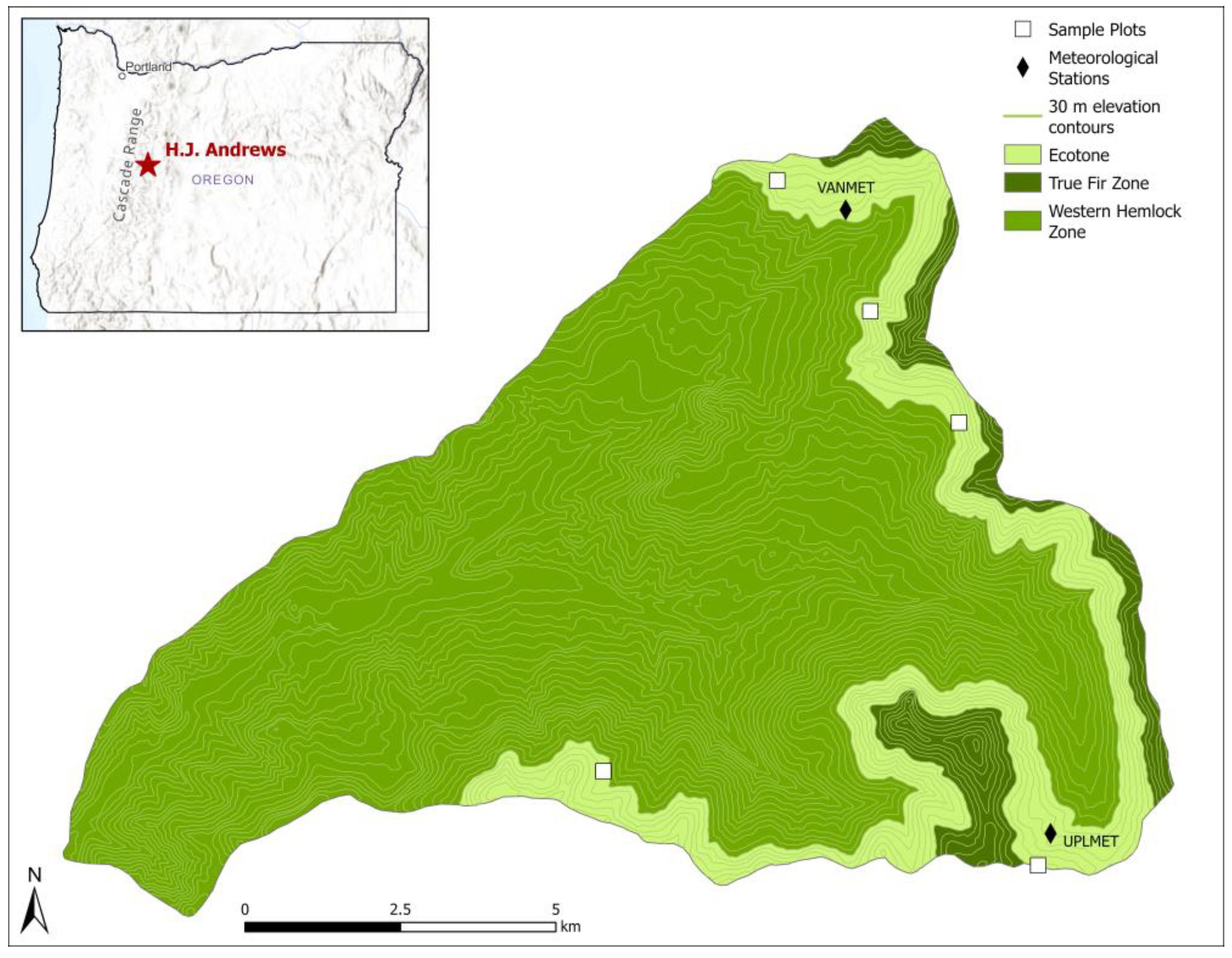
The H.J. Andrews (HJA) Experimental Forest Long-Term Ecological Research (LTER) site is located on the western slope of the Western Cascade Mountains of Oregon, USA (Figure 1). The 64 km2 HJA watershed is contained within the Willamette National Forest and spans 1200 m in elevation, from 400 m asl to 1600 m asl. The Experimental Forest was established in 1948 and added to the LTER network in 1980, so the generation and analysis of long-term datasets have a long history at the site. The site is representative of the region’s rugged mountains, stream ecosystems, and old-growth, conifer-dominated forests. Approximately 40% of the landscape could be considered old-growth, characterized by a complex stand structure containing snags, coarse woody debris, and large, old trees (in many cases over 500 years old). Lower-elevation forests are within the Western Hemlock vegetation zone, which is dominated by Tsuga heterophylla (western hemlock) with Pseudotsuga menziesii (Douglas fir) and Thuja plicata (western red cedar). The higher-elevation True Fir vegetation zone is notably colder, wetter, and snowier, and it is dominated by Abies amabilis (Pacific silver fir) and A. procera (noble fir) [29].
Oregon’s average temperature has risen by 1.2 °C since 1895 and is expected to increase by 2.8 °C by mid-century and by 4.6 °C by the 2080s in business-as-usual scenarios [30]. Precipitation has not changed substantially and winter precipitation is expected to increase slightly. However, warmer temperatures may cause more of this precipitation to fall as rain rather than snow, and annual snowpack across the state is projected to decline by 25% by 2050 [30]. Many parts of Oregon depend on seasonal meltwater, and snowpack and glacial declines will likely reduce irrigation water supplies in parts of the state. Reductions in snowpack would also contribute to declines in soil moisture, which would increase wildfire. Fire is an ever-present risk to the landscape, and large burns influenced the HJA watershed in 2020 and 2023. The 2023 Lookout Fire was particularly impactful to the HJA, having originated in it and spread over a majority of its area.
2.2. Data
Sample plots were strategically established to cross the ecotone between the Western Hemlock and True Fir vegetation types. Through prior modeling work, we used estimates of temperature [31], soil moisture [32], and radiation [33], combined with field sampling of forest composition stratified throughout the watershed, to classify and map the dominant vegetation types [34]. The model identified locations on the watershed of significant mixing of the hemlock and fir community types, and this information was used to define the ecotone for the present analysis (Figure 1). Within this ecotone band (approximately 1230 to 1410 m in elevation based on the vegetation models), we established five 20 m by 100–180 m plots for more intensive, long-term monitoring [35]. These highly heterogeneous plots represented sites on the landscape anticipated to be among the most sensitive to climate-driven ecological range shifts.
We have been monitoring changes in seedling populations within these ecotone plots since 2002. We focused on this early life stage as an indicator of species persistence or migration because of its demonstrated sensitivity to climate change and overall importance in shaping plant community dynamics [14,36,37]. Seedling data were collected in the summers of 2002, 2012, and 2022 for the following four conifer species: Tsuga heterophylla (western hemlock), Abies amabilis (Pacific silver fir), A. procera (noble fir), and A. grandis (grand fir). All seedlings up to 1.37 m tall within a 1 m offset on both sides of the plot centerlines were recorded and georeferenced. The species, height, distance along the centerline, and offset from the centerline were recorded for all seedlings on the five plots. Seedlings were binned by species and size class: young of the year (yoy), 0–10 cm in height, 10–50 cm in height, and 50–137 cm in height. Seedlings classified as yoy were later excluded from analyses due to inconsistency between years in these data. Seedling germination, growth, and therefore detectability of yoy seedlings is highly dependent on the timing of snowmelt relative to the timing of sampling. The interval between these two events was not consistent for our three vegetation surveys (2002, 2012, and 2022). We therefore excluded all the yoy seedlings from our analyses.
An average of nearly 40 elevation reference points were mapped every 20 m along the plots using an Impulse (Laser Technologies Incorporated) laser surveying system. These points were kriged to produce 1 m resolution digital elevation models (DEMs) for the plots [35]. The elevation for each seedling was then estimated by extracting the value from the DEM for the seedling’s recorded spatial locations in ArcPro®. In 2002 and 2022, we also used a spherical densiometer to record canopy cover on the plots and at observed seedling locations. For comparison purposes, publicly available elevation and snow data were also gathered from two meteorological stations (VANMET and UPLMET, canopy cover = 0 at both) located within the ecotone region of the study area (Figure 1). With the exception of A. grandis, reproductively mature trees were present on the plots in sufficient density to ensure that seeds were present and none of the species were likely dispersal-limited [35].
In 2013, we began monitoring the timing of snowmelt on the plots, and from 2013 to 2022, we recorded snow cover using data from 123 temperature data loggers (Onset HOBO Pendant Models UA-002-64), dispersed at ground level throughout the five plots. One-third of the data loggers were co-located next to T. heterophylla seedlings (20 of the loggers) and A. amabilis seedlings (24 loggers). Twenty of the loggers were located in the field of view of nine time-lapse cameras (Wingscapes TimelapseCam 8.0), which were used to validate our logger-based estimates of snow.
Measurements of temperature were recorded by the data loggers every 6 h (3:00, 9:00, 15:00, and 21:00 PST; Pacific Standard Time = Universal Time-8 h). Due to the insulating properties of snow, data loggers covered by snow recorded a consistent temperature between −1 and 1 °C. To account for times when temperatures were naturally within that range and snow was not on the ground, a “snow-covered” value for a data logger at a specific time was only recorded when the data logger recorded temperatures within that range for at least 4 consecutive readings (i.e., 24 h). When the location became snow-free, the data logger was no longer covered by snow and temperatures would fluctuate between measurements. The number of snow days metric was calculated as the number of snow-covered values for a data logger divided by 4 (4–7 snow values = 1 snow day, 8–11 snow values = 2 snow days, etc.). The last day of snow metric was calculated as the date of the final snow-covered value for a data logger. Any data loggers that stopped logging or became non-operational before the end of the snow season for that year were excluded from that year’s data.
For the validation, the “snow-covered/snow-free” classified values at 9:00 PST for all data loggers within view of a camera were compared to camera photos taken at 9:00 PST on the same day. This process involved manually inspecting over 12,000 photos: if the data logger was visible upon observation, that observation was recorded as snow-free, and otherwise, the logger was considered snow-covered. The manual observations of photos were compared to the data logger observations derived via temperature (methodology outlined in the previous paragraph), and this comparison was used to evaluate whether the data logger-based estimates were reliable indicators of the presence or absence of snow using the kappa statistic from a confusion matrix. Out of the four times when “snow-covered/snow-free” values were recorded by data loggers, only the 9:00 PST and 15:00 PST values could be used for validation since camera photos were only available during these daylight hours. The 9:00 PST values were chosen for validation somewhat arbitrarily to obtain one measurement per day. We did not validate both times every day due to our sufficiently large sample size (12,000+) and the significant labor cost of analyzing 12,000 additional photos by eye. Overall, we expected the validation statistics to be very similar at 9:00 PST and 15:00 PST.
2.3. Analyses
2.3.1. Snow Variability
We first validated the ability of the temperature data loggers to record snow cover. For each day of the snow depletion season, we used the methods described above to determine the presence or absence of snow for each of the ten to twenty data loggers per year that were in sight of the cameras (due to factors such as battery failure, damage, and loss, not all cameras nor data loggers were available for every year). We considered the snow depletion season as beginning on 21 March (or 20 March in a leap year) and ending on 30 June (or 29 June; [38]). We evaluated thousands of photos by eye during this time frame to confirm whether the data loggers were actually covered in snow for the date and created a confusion matrix to assess misclassifications and visualize the outcomes.
Once confident in the ability of the data loggers to record snow, we began to construct snow cover time series specific to the ecotone. For each year and each logger, we used the following two metrics to quantify the snow as described in Kostadinov and Lookingbill [25]:
- Number of snow days—the total number of days during the snow depletion season that the data logger was covered by snow;
- Last day of snow—the last day of the water year (which ends on 30 September) in which the data logger was covered by snow.
We calculated the number of snow days and last day of snow for each year for all available data loggers over the 10-year period from 2013 to 2022. The data recovery rate ranged from 65 to 123 data loggers per year for a total sample size of 779 records. We conducted a Pearson correlation analysis between the two snow metrics to test whether snow persistence was spatially correlated with overall snow cover during the melt season.
To assess the temporal trend, we plotted the percentages of recovered data loggers covered with snow for each day of the snow depletion season. We then constructed box plots to assess the within- and among-year variability in the total snow days and the last day of snow metrics to examine whether snow had been decreasing or snowmelt occurring earlier in the spring over time.
To test the hypothesis that climate teleconnections due to the El Niño–Southern Oscillation (ENSO) and the Pacific Decadal Oscillation (PDO) were drivers of snow cover variability in the ecotone during the melt season, monthly values for the multivariate ENSO index (MEI) [39,40] and the PDO index [41,42] were obtained for 2013–2022. Yearly ENSO averages were calculated using ENSO values from December to February right before the snow depletion season of that year while yearly PDO averages were calculated using PDO values from October to March, following the methods of Kostadinov and Lookingbill [25]. These two averages were combined to develop a final ENSO/PDO value for the year, which was then compared to the snow metric values for each year using ordinary least squares (OLS) linear regression.
2.3.2. Forest Regeneration
To test whether species were well mixed within the ecotone, we conducted a Wilcoxon rank sum test comparing the cumulative frequency distributions of abundance based on elevation for the observed T. heterophylla and A. amabilis seedlings. To test whether seedlings shifted to higher elevations over the 20-year study period, we conducted Kruskal–Wallis tests on the abundance distributions for the three sample years (2002, 2012, 2022) for both species. To test whether the timing of snowmelt was spatially correlated with seedling composition, we calculated the average number of snow days and average last day of snow for the 44 data loggers located at 24 A. amabilis and 20 T. heterophylla seedlings. We compared the overall and yearly averages of the snow metrics for the two seedling types using Wilcoxon rank sum tests to determine if either of the two metrics significantly predicted differences in the locations of the two species.
Data sorting and manipulation was performed in Python. All statistical tests were conducted in R (R Core Team, 2023).
3. Results
3.1. Snow Variability
The data loggers were reliable measures of the presence or absence of snow at their fixed locations during the snow depletion season. Of the 12,357 measurements pairing data logger assessments of snow presence–absence with the presence–absence observations derived from the photos, 12,030 were a match (kappa = 0.94). False-negative Type II errors (n = 186) slightly exceeded false-positive Type I errors (n = 141), but both were negligible (Table 1).
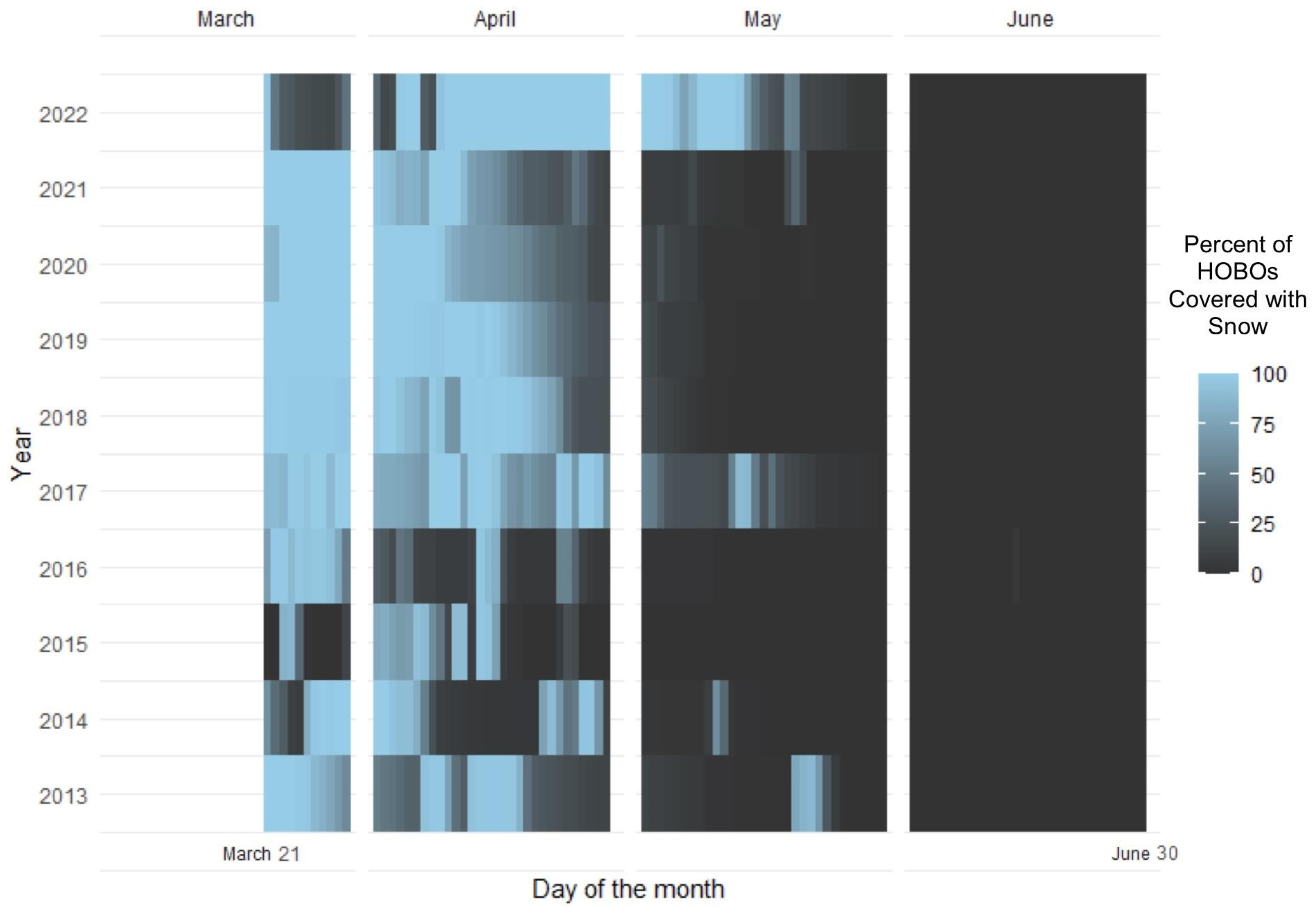
In total, we recorded an average of 28.6 snow days per year from 2013 to 2022 across all plots and all sensors (Figure 2; recall that snow days were counted for the melt season beginning on 20 or 21 March). The number of snow days ranged from a low of 13.0 days/sensor in 2015 to a high of 44.8 days/sensor in 2022. The mean last day of snow from 2013 to 2022 (and across all loggers) was 2 May; the annual mean (across all loggers) ranged from 17 April to 18 May over the study period.
The amount of snow on the plots was consistently less than at the neighboring meteorological stations, which can be explained by the differences in canopy cover. In 2022, the total number of snow days recorded by the different data loggers ranged from 35 to 72, and the canopy cover over those sensors ranged from 37.5% to 99% (mean = 85.4%). In contrast, the two meteorological stations are located in open field conditions (0% canopy cover) and recorded 80 (at UPLMET) and 102 snow days (at VANMET) for the 2022 snow depletion season. The relationship between canopy cover and number of snow days was highly significant for the 2022 data loggers (R2 = 0.32; p < 0.001). From 2002 to 2022, there was minimal disturbance to the canopy on the plots. Canopy cover decreased slightly from an average plot value of 94% to 85%, most of which was caused by treefall disturbance on one of the plots resulting in a decrease from 95% to 79% on that plot.
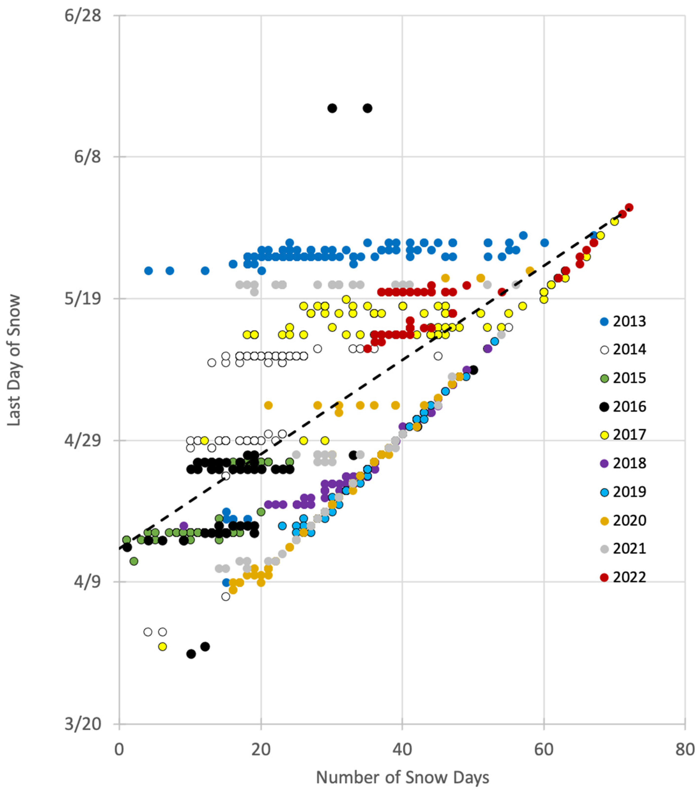
Across all years, from 2013 to 2022, the day of snow disappearance metric was significantly correlated (r = 0.54; n = 820, p < 0.001) with the total number of snow days metric (Figure 3). For some years, the metrics provided nearly identical information (e.g., r = 0.99 in 2019 and r = 0.92 in 2020, p <0.001); for other years, the correlation was much weaker (e.g., r = 0.28 in 2021, p = 0.03). For simplicity, the remaining figures below are provided for the total number of snow days metric. However, results are reported in the text for both metrics.
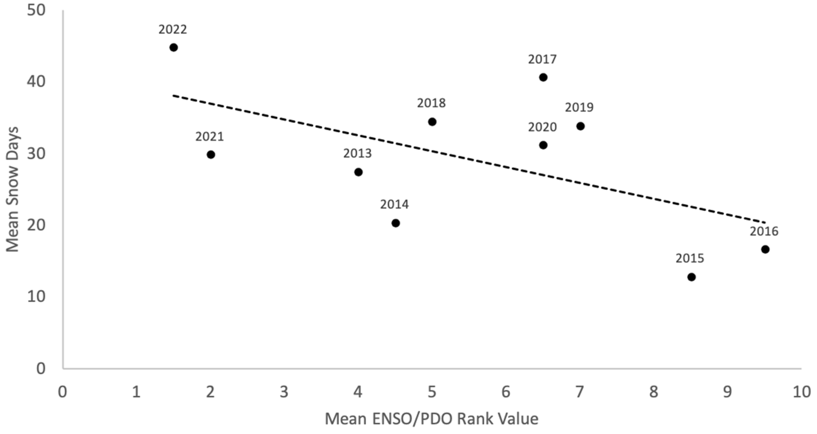
The time series of the number of snow days metric illustrates the high interannual variability at the site (Figure 4), which is also notable in Figure 3, and is consistent with the results of Kostadinov and Lookingbill [25], who also observed high interannual variability in snow cover and disappearance dates for this ecotone. In general, the second half of the decade had more snow, with the snowiest year being the most recent (2022). The least snowy years were 2014–2016. Any long-term signal was obscured by ENSO, PDO, and other sources of variability over this time period. Cold-phase years of ENSO/PDO were correlated with more snow days (R2 = 0.32; p = 0.08), which can explain the high amounts of snow in the most recent years. The two years with the warmest ENSO/PDO states were also the two least snowy years (Figure 5).
3.2. Forest Regeneration
Of the four species of seedlings recorded, T. heterophylla (n = 829) and A. amabilis (n = 781) were found most frequently in the ecotone (Table 2). Over 80% of the T. heterophylla seedlings were located on nurse logs, while only a small fraction of the A. amabilis and A. procera seedlings were located on nurse logs. Totaling across all years, the T. heterophylla seedlings (median 1285 m) were observed at significantly (p < 0.001) lower elevations than the A. amabilis seedlings (median 1337 m). Cumulative frequency distributions for the two species’ seedling elevations are provided in Figure 6.
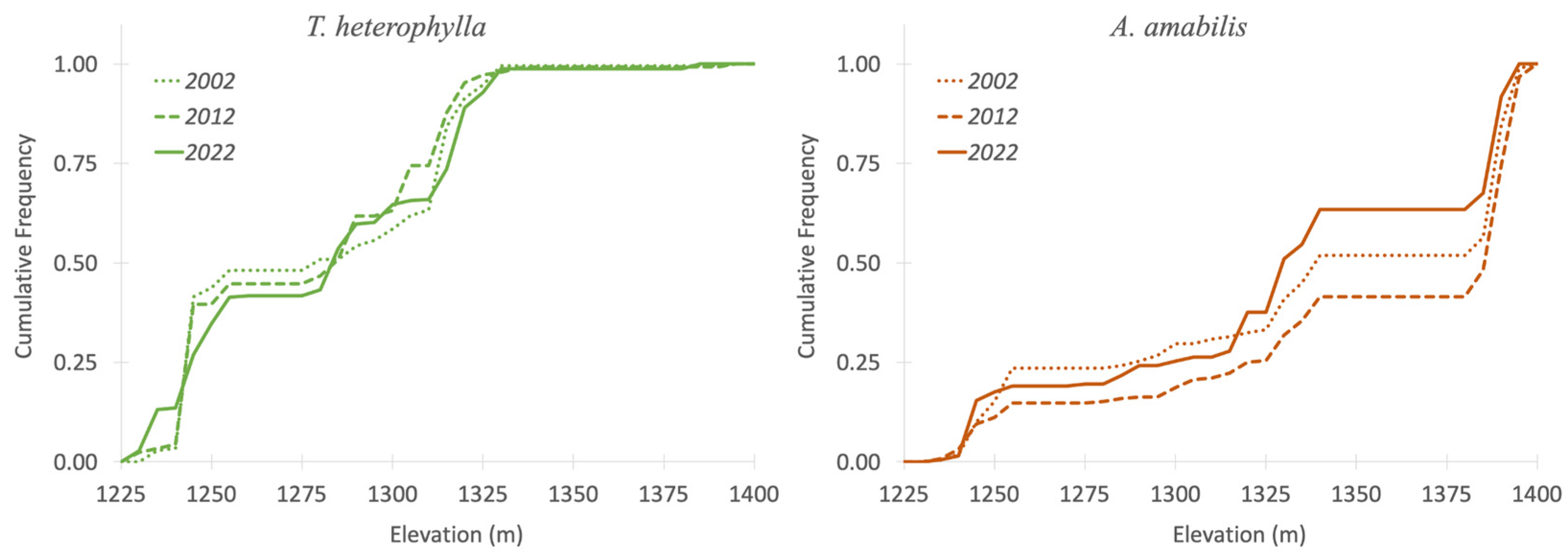
A comparison among years (2002, 2012, and 2022) revealed no significant upslope shift of seedlings for either species (p > 0.05) based on the Kruskal–Wallis tests (Figure 7). Median elevation for the T. heterophylla seedlings was 1279 m in 2002 and 1285 m in 2022. Median elevation for the A. amabilis seedlings was 1337 m in 2002 and 1328 m in 2022.
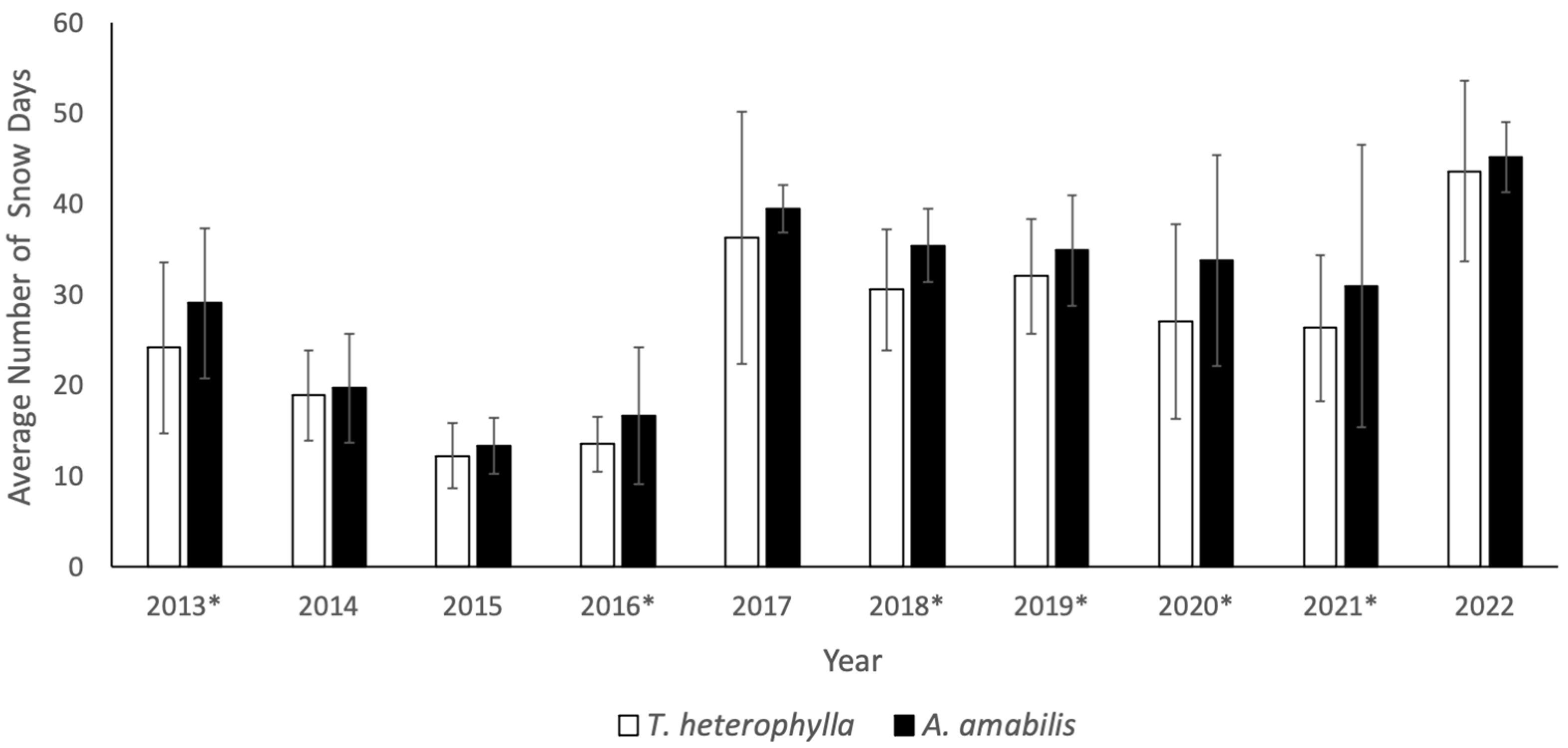
On average, four fewer snow days per year were recorded by data loggers located at T. heterophylla seedling locations (mean = 27 days) compared to data loggers located at A. amabilis seedling locations (mean = 31 days, p = 0.021). Differences were significant for six of the 10 individual years (Figure 8). Generally, differences were not significant in the years of highest (2017 and 2022) and lowest snow cover (2014 and 2015, but significant for 2016). Differences between the two species were also not significant for the last day of snow metric (p = 0.55), with the average date of the last snowmelt from 2013 to 2022 for the T. heterophylla and A. amabilis seedlings occurring on 2 May and 3 May, respectively.
4. Discussion
Our results suggest that relatively inexpensive temperature data loggers offer a highly reliable option for detecting the presence or absence of snow cover at decadal time scales. Agreement with time-lapse camera observations was strong, though the malfunction and loss of loggers in the harsh field conditions of the HJA were appreciable. Overall, using a network of inexpensive temperature loggers on the forest floor to detect snow presence provides a useful complement to satellite-, airborne-, and lidar-based mapping of snow dynamics in remote and difficult-to-access landscapes. This approach has the distinct advantage that it is affordable and collects time series for a long period of time with minimal maintenance, requiring no local power or internet infrastructure. The basic principle of operation of the snow detection employed here (using the insulating properties of the snow) has been shown to be effective and accurate by other investigators as well and can also be used with a fiber optic cable to detect snow along long linear pathways [26,43,44]. Combined with light sensors and aligned in vertical distributions, temperature data loggers can even be used to detect snow depth at a low cost in remote locations [45].
In forested landscapes, the approach provides the added benefit of measuring conditions below tree canopies and at fine spatial scales that may be important to forest processes such as seedling germination and establishment, as well as for developing and validating remote sensing algorithms for the detection of snow under a canopy (e.g., [26]). Our estimates from the temperature data loggers under the canopy at the HJA generally indicated an earlier melt and lower total snow amounts than provided by nearby meteorological stations located in open fields. Two of the years (2013 and 2014) from our study overlapped with those of an earlier study that used MODIS satellite-based methods to assess snow for the same Western Hemlock–True Fir ecotone but over a larger geographic region [25]. Using the methods from that study to assign snow days to the ecotone, our two studies are in agreement about whether the ecotone was snow-covered or not for 177 out of the 204 days (87%) in the snow depletion seasons for the two years. Two late-season storms (one each year in May) that occurred after the initial melt-off for the year resulted in a total of seven snow days that were captured by the field data loggers but not by the satellite imagery. Additionally, the satellite record included nine consecutive “snow days” in April 2014 that were assessed as snow-free by the data loggers. These comparisons with local meteorological and remote sensing data suggest the following: (a) snow dynamics under a canopy are different than they are in the open, as expected [26], and (b) as stated above, the network of temperature loggers under a canopy provides very useful and complementary information to other remote and in situ methods of snow observation.
Apart from the modality of measurement, the choice of snow metrics is another important decision in understanding the impact of changes in snowfall and melt on snow-adapted species. For example, here, we demonstrated that the number of snow days and the snow disappearance date did not exhibit a perfect correlation. At a much larger scale, Pierce & Cayan [1] compared different snow metrics in their ability to detect a statistically significant, multi-decadal trend from climate models for the western United States. While they found that many of the variables that they investigated such as snow season length were generally changing as a result of climate change, they reported an uneven response among the different metrics. Ultimately, different stakeholders may select different metrics based on the intended use and the sensitivity of the studied entity or question to the metrics.
For our purposes, the last day of snowmelt and the total number of snow days during the snow depletion season were selected as two metrics with potential relevance to the regeneration niche of our species of concern. The two metrics were moderately correlated for most but not all years. We found a significant difference in the first of these metrics between the two seedling species (mean = 27 snow days for the T. heterophylla seedlings; mean = 31 snow days for the A. amabilis seedlings), supporting the suggestion that the stiffer A. amabilis seedlings may be more tolerant to spring snows and that the influence of snow might be critical to shaping this ecotone [46,47]. However, we did not observe a significant difference in terms of the timing of snow disappearance, which was more sensitive, for example, to late-season storms that would cover all of the sensors for a day or two but likely not have a lasting impact on the forest physiology or hydrology.
Despite the global increases in temperature, the HJA has exhibited only limited evidence of warming, e.g., local observations of earlier springs in some areas of the landscape [48]. We found that neither snow metric significantly decreased over the period of study. Instead, climate oscillations such as ENSO and PDO appear to be the dominant drivers of snow variability at this temporal scale. The recorded correlation with negative phases of ENSO (La Niña) (more snow in negative ENSO years) is consistent with other findings in Pacific mountains including instrument and reconstructed snowpacks from 300 years of tree ring data in British Columbia [8]. Although we did not observe a temporal decrease in snow cover over the past decade, the observed differences in the mean number of snow days for the A. amabilis and T. heterophylla seedling locations could have important climate change implications. Any future changes in snow (e.g., even through indirect pathways by impacting the strength and/or frequency of ENSO/PDO events) are likely to have significant impacts on the composition of these forests.
Given the lack of a trend in the snow data, it is perhaps not surprising that we did not find that seedling distributions within the ecotone were consistently shifting to higher elevations. We also note that for some earth system datasets, many years or decades of data would be required to distinguish a long-term trend from natural noise (e.g., [25]), especially given that gaps/discontinuities in sensors and data are common and even inevitable [49,50]. It may also be the case that climate trends may not necessarily be the best predictor of species range shifts driven by differential seedling establishment [51]. Because regeneration events happen over discrete periods of time, “windows of opportunity” in which conditions are ripe for seedling survival over a small number of consecutive years may be a better indicator of species’ response to climate change [37]. Accordingly, two years of cooler, wetter weather from 2020 to 2022 may have provided the window of opportunity conditions necessary to support species persistence in their current niches despite longer-term global warming [52]. After multiple La Niña years, 2023/2024 ushered in an El Niño, with a shift to yet another La Niña likely by mid-2024. It will be important to continue to track the consequences of these episodic events on the regeneration of these forests.
Other recent studies have found similar stability in tree species ranges over the past decades, but have highlighted the potential effect of increases in disturbance events in triggering range shifts [53]. The possible triggering effect of disturbances such as fire, which are likely to become more frequent as a consequence of warming and earlier spring snowmelt [15], requires additional study. For example, many long-term studies at the HJA, such as this one, have been majorly disrupted by the summer 2023 Lookout Fire that burned much of the Experimental Forest. The fire offers a potential opportunity for new seedling establishment within the ecotone. The consequences of this fire should be closely monitored. Though we did not observe substantial range shifts within these old-growth stands, the interaction of climate and fire may result in future patterns of seedling establishment that drive landscape change [54,55].
It is also possible that microsite topographic variability and neighborhood effects are more important in determining species distributions than elevation at the ecotone level [56]. Alatalo and Ferrarini [57] demonstrated how topography can slow the upslope shift of subalpine forests. Although the strong association between fallen overstory trees (nurse logs) and T. heterophylla regeneration has been well documented in these forests (e.g., [58]), the mechanism underlying this association is not clearly understood, as coarse woody debris is a relatively nutrient-poor substrate compared to the forest floor [59]. We found that over 80% of T. heterophylla seedlings in the ecotone were located on nurse logs, which are also likely to affect snow dynamics as compared to ground locations. More research is needed on these relationships and their interactions with climate migration to develop effective adaptation strategies for forests of the Northwestern USA [60].
5. Conclusions
The results provided here highlight the importance of below-canopy, fine-resolution snow measurements to understand snow dynamics relevant to forest processes like seedling recruitment. Such data are also important for the development of remote-sensing algorithms capable of accounting for differences in under-canopy vs. open/gap area snow dynamics in forests. The results confirm the strong influence of climatic oscillations on montane old-growth forests. As global climate change alters abiotic factors in ways that are often hard to predict at landscape scales, long-term studies will continue to be essential in providing valuable information on the resilience of old-growth forests. Ultimately, combining remote sensing and local field plot data may be the best way to monitor changes in forest ecotones over decadal time scales.
Author Contributions
Conceptualization, T.R.L.; methodology, T.R.L. and T.S.K.; investigation, T.R.L., J.D., E.J., M.G. and T.S.K.; formal analysis, T.R.L., J.D., E.J. and M.G.; data curation, J.D.; validation, M.G.; visualization, J.D., E.J. and M.G.; software, J.D.; supervision, T.R.L.; project administration, T.R.L.; writing—original draft preparation, T.R.L.; writing—review and editing, J.D., E.J., M.G. and T.S.K. All authors have read and agreed to the published version of the manuscript.
Funding
This work was supported by the University of Richmond School of Arts and Sciences, the Associated Colleges of the South Andrew W. Mellon Environmental Fellowship, and the H.J. Andrews Experimental Forest and Long-Term Ecological Research (LTER) program under the NSF Grant No. LTER8 DEB-2025755. TSK also acknowledges support from California State University San Marcos.
Data Availability Statement
All original data that support the findings of this study are available from the corresponding author upon reasonable request. The raw data logger and camera data along with the scripts used in the analyses of these datasets are available at https://github.com/jbdupuy/HJA_Research.git. Meteorological data are available at the HJ Andrews Experimental Forest database https://andrewsforest.oregonstate.edu/data (accessed on 11 July 2022).
Acknowledgments
Thank you to Charles Mullis for his assistance with the preliminary analyses of these datasets. Conor Phelan, Andrew Pericak, Ethan Strickler, Sanitra Desai, Monica Stack, Adam Owens, Claire Goelst, and Sarah Ward assisted with data collection. Beth Zizzamia provided technical assistance. We are particularly grateful to Mark Schulze who provided advice and support throughout the study.
Conflicts of Interest
The authors declare no conflicts of interest.
References
- Pierce, D.; Cayan, D. The uneven response of different snow measures to human-induced climate warming. J. Clim. 2013, 26, 4148–4167. [Google Scholar] [CrossRef]
- Rhoades, A.M.; Jones, A.D.; Ullrich, P.A. The changing character of the California Sierra Nevada as a natural reservoir. Geophys. Res. Lett. 2018, 45, 8–13. [Google Scholar] [CrossRef]
- Ikeda, K.; Rasmussen, R.; Liu, C.; Newman, A.; Chen, F.; Barlage, M.; Gutmann, E.; Dudhia, J.; Dai, A.; Luce, C.; et al. Snowfall and snowpack in the Western U.S. as captured by convection permitting climate simulations: Current climate and pseudo global warming future climate. Clim. Dyn. 2021, 57, 2191–2215. [Google Scholar] [CrossRef]
- Beniston, M. Climatic change in mountain regions: A review of possible impacts. Clim. Change 2003, 59, 5–31. [Google Scholar] [CrossRef]
- Sproles, E.A.; Nolin, A.W.; Rittger, K.; Painter, T.H. Climate change impacts on maritime mountain snowpack in the Oregon Cascades. Hydrol. Earth Syst. Sci. 2013, 17, 2581–2597. [Google Scholar] [CrossRef]
- Mazzotti, G.; Webster, C.; Quéno, L.; Cluzet, B.; Jonas, T. Canopy structure, topography, and weather are equally important drivers of small-scale snow cover dynamics in sub-alpine forests. Hydrol. Earth Syst. Sci. 2023, 27, 2099–2121. [Google Scholar] [CrossRef]
- Dickerson-Lange, S.E.; Gersonde, R.F.; Hubbart, J.A.; Link, T.E.; Nolin, A.W.; Perry, G.H.; Roth, T.R.; Wayand, N.E.; Lundquist, J.D. Snow disappearance timing is dominated by forest effects on snow accumulation in warm winter climates of the Pacific Northwest, United States. Hydrol. Process. 2017, 31, 1846–1862. [Google Scholar] [CrossRef]
- Mood, B.J.; Coulthard, B.; Smith, D.J. Three hundred years of snowpack variability in southwestern British Columbia reconstructed from tree-rings. Hydrol. Process. 2020, 34, 5123–5133. [Google Scholar] [CrossRef]
- Jump, A.S.; Mátyás, C.; Peñuelas, J. The altitude-for-latitude disparity in the range retractions of woody species. Trends Ecol. Evol. 2009, 24, 694–701. [Google Scholar] [CrossRef]
- Breshears, D.D.; Huxman, T.E.; Adams, H.D.; Davison, J.E. Vegetation synchronously leans upslope as climate warms. Proc. Natl. Acad. Sci. USA 2008, 105, 11591–11592. [Google Scholar] [CrossRef]
- Vitasse, Y.; Ursenbacher, S.; Klein, G.; Bohnenstengel, T.; Chittaro, Y.; Delestrade, A.; Monnerat, C.; Rebetez, M.; Rixen, C.; Strebel, N.; et al. Phenological and elevational shifts of plants, animals and fungi under climate change in the European Alps. Biol. Rev. Camb. Philos. Soc. 2021, 96, 1816–1835. [Google Scholar] [CrossRef] [PubMed]
- Freeman, B.G.; Lee-Yaw, J.A.; Sunday, J.M.; Hargreaves, A.L. Expanding, shifting, and shrinking: The impact of global warming on species’ elevational distributions. Glob. Ecol. Biogeogr. 2018, 27, 1268–1276. [Google Scholar] [CrossRef]
- Spies, T.A.; Giesen, T.W.; Swanson, F.J.; Franklin, J.F.; Lach, D.; Johnson, K.N. Climate change adaptation strategies for federal forests of the Pacific Northwest, USA: Ecological, policy, and socio-economic perspectives. Landsc. Ecol. 2010, 25, 1185–1199. [Google Scholar] [CrossRef]
- Hagedorn, B.; Flower, A. Conifer establishment and encroachment on subalpine meadows around Mt. Baker, WA, USA. Forests 2021, 12, 1390. [Google Scholar] [CrossRef]
- Westerling, A.L.; Hidalgo, H.G.; Cayan, D.R.; Swetnam, T.W. Warming and earlier spring snowmelt increase western US forest fire activity. Science 2006, 313, 949–952. [Google Scholar] [CrossRef] [PubMed]
- Contosta, A.R.; Casson, N.J.; Garlick, S.; Nelson, S.J.; Ayres, M.P.; Burakowski, E.A.; Campell, J.; Creed, I.; Eimers, C.; Evans, C.; et al. Northern forest winters have lost cold, snowy conditions that are important for ecosystems and human communities. Ecol. Appl. 2019, 29, e01974. [Google Scholar] [CrossRef] [PubMed]
- Kueppers, L.M.; Conlisk, E.; Castanha, C.; Moyes, A.B.; Germino, M.J.; de Valpine, P.; Torn, M.S.; Mitton, J.B. Warming and provenance limit tree recruitment across and beyond the elevation range of subalpine forest. Glob. Change Biol. 2016, 23, 2383–2395. [Google Scholar] [CrossRef] [PubMed]
- Werner, C.M.; Young, D.J.N.; Safford, H.D.; Young, T.P. Decreased snowpack and warmer temperatures reduce the negative effects of interspecific competitors on regenerating conifers. Oecologia 2019, 191, 731–743. [Google Scholar] [CrossRef]
- Ford, K.R.; HilleRisLambers, J. Soil alters seedling establishment responses to climate. Ecol. Lett. 2019, 23, 140–148. [Google Scholar] [CrossRef]
- Kark, S. Ecotones and ecological gradients. In Ecological Systems; Leemans, R., Ed.; Springer: New York, NY, USA, 2012; pp. 147–160. [Google Scholar]
- Wasson, K.; Woolfolk, A.; Fresquez, C. Ecotones as indicators of changing environmental conditions: Rapid migration of salt marsh-upland boundaries. Estuaries Coasts 2013, 36, 654–664. [Google Scholar] [CrossRef]
- Nelson, K.N.; O’Dean, E.; Knapp, E.E.; Parker, A.J.; Bisbing, S.M. Persistent yet vulnerable: Resurvey of an Abies ecotone reveals few differences but vulnerability to climate change. Ecology 2021, 102, e03525. [Google Scholar] [CrossRef] [PubMed]
- Dearborn, K.D.; Danby, R.K. Spatial analysis of forest-tundra ecotones reveals the influence of topography and vegetation on alpine treeline patterns in the subarctic. Ann. Am. Assoc. Geogr. 2019, 110, 18–35. [Google Scholar] [CrossRef]
- Gleason, K.E.; Nolin, A.W.; Roth, T.R. Developing a representative snow-monitoring network in a forested mountain watershed. Hydrol. Earth Syst. Sci. 2017, 21, 1137–1147. [Google Scholar] [CrossRef]
- Kostadinov, T.S.; Lookingbill, T.R. Snow cover variability in a forest ecotone of the Oregon Cascades via MODIS Terra products. Remote Sens. Environ. 2015, 164, 155–169. [Google Scholar] [CrossRef]
- Kostadinov, T.S.; Schumer, R.; Hausner, M.; Bormann, K.J.; Gaffney, R.; McGwire, K.; Painter, T.H.; Tyler, S.; Harpold, A.A. Watershed-scale mapping of fractional snow cover under conifer forest canopy using lidar. Remote Sens. Environ. 2019, 222, 34–49. [Google Scholar] [CrossRef]
- De Frenne, P.; Zellweger, F.; Rodríguez-Sánchez, F.; Scheffers, B.R.; Hylander, K.; Luoto, M.; Vellend, M.; Verheyen, K.; Lenoir, J. Global buffering of temperatures under forest canopies. Nat. Ecol. Evol. 2019, 3, 744–749. [Google Scholar] [CrossRef] [PubMed]
- Aulló-Maestro, I.; Gómez, C.; Hernández, L.; Camarero, J.J.; Sánchez-González, M.; Cañellas, I.; de la Cueva, A.V.; Montes, F. Monitoring montane-subalpine forest ecotone in the Pyrenees through sequential forest inventories and Landsat imagery. Ann. For. Sci. 2023, 80, 32. [Google Scholar] [CrossRef]
- Franklin, J.F.; Dyrness, C.T. Natural Vegetation of Oregon and Washington; Oregon State University Press: Corvallis, OR, USA, 1988. [Google Scholar]
- Fleishman, E. (Ed.) Sixth Oregon Climate Assessment; Oregon Climate Change Research Institute, Oregon State University: Corvallis, OR, USA, 2023; Available online: https://blogs.oregonstate.edu/occri/oregon-climate-assessments (accessed on 30 June 2023).
- Lookingbill, T.R.; Urban, D.L. Spatial estimation of air temperature differences for landscape-scale studies in montane environments. Agric. For. Meteorol. 2003, 114, 141–151. [Google Scholar] [CrossRef]
- Lookingbill, T.; Urban, D. An empirical approach towards improved spatial estimates of soil moisture for vegetation analysis. Landsc. Ecol. 2004, 19, 417–433. [Google Scholar] [CrossRef]
- Pierce, K.B.; Lookingbill, T.; Urban, D. A simple method for estimating potential relative radiation (PRR) for landscape-scale vegetation analysis. Landsc. Ecol. 2005, 20, 137–147. [Google Scholar] [CrossRef]
- Lookingbill, T.R.; Urban, D.L. Gradient analysis, the next generation: Towards more plant-relevant explanatory variables. Can. J. For. Res. 2005, 35, 1744–1753. [Google Scholar] [CrossRef]
- Lookingbill, T.R.; Rocca, M.E.; Urban, D.L. Focused assessment of scale-dependent vegetation pattern. In Predictive Species and Habitat Modeling in Landscape Ecology; Drew, C.A., Wiersma, Y., Huettmann, F., Eds.; Springer: New York, NY, USA, 2010; pp. 111–138. [Google Scholar]
- Grubb, P.J. The maintenance of species-richness in plant communities: The importance of the regeneration niche. Biol. Rev. Camb. Philos. Soc. 1977, 52, 107–145. [Google Scholar] [CrossRef]
- Serra-Diaz, J.M.; Franklin, J.; Sweet, L.C.; McCullough, I.M.; Syphard, A.D.; Regan, H.M.; Flint, L.E.; Flint, A.L.; Dingman, J.R.; Moritz, M.A.; et al. Averaged 30 year climate change projections mask opportunities for species establishment. Ecography 2016, 39, 844–845. [Google Scholar] [CrossRef]
- Hall, D.K.; Foster, J.L.; DiGirolamo, N.; Riggs, G.A. Snow cover, snowmelt timing and stream power in the Wind River Range, Wyoming. Geomorphology 2012, 137, 87–93. [Google Scholar] [CrossRef]
- Wolter, K.; Timlin, M.S. Monitoring ENSO in COADS with a seasonally adjusted principal component index. In Proceedings of the 17th Climate Diagnostics Workshop, Norman, OK, USA, 18–23 October 1992; pp. 52–57. [Google Scholar]
- Wolter, K.; Timlin, M.S. Measuring the strength of ENSO events: How does 1997/1998 rank? R. Meteorol. Soc. 1998, 53, 315–324. [Google Scholar]
- Mantua, N.J.; Hare, S.R.; Zhang, Y.; Wallace, J.M.; Francis, R.C. A pacific interdecadal climate oscillation with impacts on salmon production. Bull. Am. Meteorol. Soc. 1997, 78, 1069–1080. [Google Scholar] [CrossRef]
- Zhang, Y.; Wallace, J.M.; Battisti, D.S. ENSO-like interdecadal variability. J. Clim. 1997, 10, 1004–1020. [Google Scholar] [CrossRef]
- Tyler, S.W.; Selker, J.S.; Hausner, M.B.; Hatch, C.E.; Torgersen, T.; Thodal, C.E.; Schladow, S.G. Environmental temperature sensing using Raman spectra DTS fiber-optic methods. Water Resour. Res. 2009, 45, W00D23. [Google Scholar] [CrossRef]
- Raleigh, M.S.; Rittger, K.; Moore, C.E.; Henn, B.; Lutz, J.A.; Lundquist, J.D. Ground-based testing of MODIS fractional snow cover in subalpine meadows and forests of the Sierra Nevada. Remote Sens. Environ. 2013, 128, 44–57. [Google Scholar] [CrossRef]
- Tutton, R.J.; Way, R.G. A low-cost method for monitoring snow characteristics at remote field sites. Cryosphere 2021, 15, 1–15. [Google Scholar] [CrossRef]
- Thornburgh, D.A. Dynamics of the True Fir-Hemlock Forests of the West Slope of the Washington Cascade Range; University of Washington: Seattle, WA, USA, 1969. [Google Scholar]
- Mori, A.S.; Mizumachi, E.; Sprugel, D.G. Morphological acclimation to understory environments in Abies amabilis, a shade- and snow-tolerant conifer species of the Cascade Mountains, Washington, USA. Tree Physiol. 2008, 28, 815–824. [Google Scholar] [CrossRef]
- Jones, J.A.; Creed, I.F.; Hatcher, K.L.; Warren, R.J.; Adams, M.B.; Benson, M.H.; Boose, E.; Brown, W.A.; Campell, J.L.; Covich, A.; et al. Ecosystem processes and human influences regulate streamflow response to climate change at long-term ecological research sites. BioScience 2012, 62, 390–404. [Google Scholar] [CrossRef]
- Weatherhead, E.C.; Reinsel, G.C.; Tiao, G.C.; Meng, X.; Choi, D.; Cheang, W.; Keller, T.; DeLuisi, J.; Wuebbles, D.J.; Kerr, J.B.; et al. Factors affecting the detection of trends: Statistical considerations and applications to environmental data. J. Geophys. Res. 1998, 103, 17149–17161. [Google Scholar] [CrossRef]
- Beaulieu, C.; Henson, S.A.; Sarmiento, J.L.; Dunne, J.P.; Doney, S.C.; Rykaczewski, R.R.; Bopp, L. Factors challenging our ability to detect long-term trends in ocean chlorophyll. Biogeosciences 2013, 10, 2711–2724. [Google Scholar] [CrossRef]
- Brown, C.D.; Vellend, M. Non-climatic constraints on upper elevational plant range expansion under climate change. R. Soc. Biol. 2014, 281, 20141779. [Google Scholar] [CrossRef] [PubMed]
- Hannah, L.; Flint, L.; Syphard, A.D.; Moritz, M.A.; Buckley, L.B.; McCullough, I.M. Fine-grain modeling of species’ response to climate change: Holdouts, stepping-stones, and microrefugia. Trends Ecol. Evol. 2014, 29, 390–397. [Google Scholar] [CrossRef] [PubMed]
- Bonannella, C.; Parente, L.; de Bruin, S.; Herold, M. Multi-decadal trend analysis and forest disturbance assessment of European tree species: Concerning signs of a subtle shift. For. Ecol. Manag. 2024, 554, 121652. [Google Scholar] [CrossRef]
- Smith, A.L.; Blair, D.; McBurney, L.; Banks, S.C.; Barton, P.S.; Blanchard, W.; Driscoll, D.A.; Gill, A.M.; Lindenmayer, D.B. Dominant drivers of seedling establishment in a fire-dependent obligate seeder: Climate or fire regimes? Ecosystems 2014, 17, 258–270. [Google Scholar] [CrossRef]
- Liang, S.; Hurteau, M.D. Novel climate-fire-vegetation interactions and their influence on forest ecosystems in the western USA. Funct. Ecol. 2023, 37, 2126–2142. [Google Scholar] [CrossRef]
- Lippok, D.; Beck, S.G.; Renison, D.; Hensen, I.; Apaza, A.E.; Schleuning, M. Topography and edge effects are more important than elevation as drivers of vegetation patterns in a neotropical montane forest. J. Veg. Sci. 2013, 25, 724–733. [Google Scholar] [CrossRef]
- Alatalo, J.M.; Ferrarini, A. Braking effect of climate and topography on global change-induced upslope forest expansion. Int. J. Biometeorol. 2016, 61, 541–548. [Google Scholar] [CrossRef] [PubMed]
- Gray, A.N.; Spies, T.A. Microsite controls on tree seedling establishment in conifer forest canopy gaps. Ecology 1997, 78, 2458–2473. [Google Scholar] [CrossRef]
- Harmon, M.E.; Franklin, J.F.; Swanson, F.J.; Sollins, P.; Gregory, S.V.; Lattin, J.D.; Anderson, N.H.; Cline, S.P.; Aumen, N.G.; Sedell, J.R.; et al. Ecology of coarse woody debris in temperate ecosystems. Adv. Ecol. Res. 2004, 34, 59–234. [Google Scholar]
- Halofsky, J.E.; Peterson, D.L. Climate change vulnerabilities and adaptation options for forest vegetation management in the Northwestern USA. Atmosphere 2016, 7, 46. [Google Scholar] [CrossRef]
Figure 1.
The H.J. Andrews Experimental Forest study watershed. The light green band represents an elevation-based approximation (1230–1410 m) of the Western Hemlock–True Fir ecotone. Sample plots are marked by white boxes. Diamonds indicate locations of two benchmark meteorological stations located in the ecotone: Vanilla Leaf (elevation = 1275 m) and Upper Lookout (elevation = 1295 m). Inset: the star identifies the location of H.J. Andrews in Oregon, USA. The map projection is NAD83 UTM Zone 10N.

Figure 2.
Percentages of data loggers covered by snow for each day of the snow depletion seasons from 2013 to 2022. Within this timeframe, 2022 had the most days with snow cover, while 2015 had the fewest number of snow days.
Figure 2.
Percentages of data loggers covered by snow for each day of the snow depletion seasons from 2013 to 2022. Within this timeframe, 2022 had the most days with snow cover, while 2015 had the fewest number of snow days.

Figure 3.
Correlation of two snow metrics, last day of snow and total number of snow days during the snow depletion season, as recorded by the forest floor temperature data loggers (2013–2022). The metrics were moderately correlated (r = 0.54; n = 820; p < 0.001), indicating that snow persistence was correlated with overall snow cover during the depletion season.

Figure 4.
Boxplot showing the medians, interquartile ranges, and outliers of the number of snow days metric by year for all data loggers (2013–2022). Years were classified as hot (red), cold (blue), or neutral (gray) based on combined ENSO and PDO rankings. The coldest ENSO/PDO year was 2022, with an ENSO value of −1.067, a PDO value of −2.422, and a median of 41 snow days per data collector. The warmest ENSO/PDO year was 2016, with an ENSO value of 1.867, a PDO value of 0.812, and a median of 14 snow days.

Figure 5.
Linear regression analysis between the mean number of snow days per year and the mean rank value from the ENSO and PDO indices for the year (R2 = 0.32; p = 0.08). High-rank values indicate the warm PDO and ENSO years; low-rank values indicate the cool phases of the PDO and ENSO.
Figure 5.
Linear regression analysis between the mean number of snow days per year and the mean rank value from the ENSO and PDO indices for the year (R2 = 0.32; p = 0.08). High-rank values indicate the warm PDO and ENSO years; low-rank values indicate the cool phases of the PDO and ENSO.

Figure 6.
Elevational sorting of species. Cumulative frequency distributions of elevation for all T. heterophylla and A. amabilis seedling abundances highlight a significant (p < 0.001) elevational difference between the two species based on Wilcoxon rank sum testing, with T. heterophylla being found at lower elevations (median = 1285 m) and A. amabilis found at higher elevations (median = 1337 m).

Figure 7.
No temporal shift in elevation. Cumulative frequency distributions of elevation by species for the three sample years (2002, 2012, 2022) indicate no significant shift for T. heterophylla seedlings or A. amabilis seedlings in the ecotone based on the Kruskal–Wallis tests (p > 0.05).
Figure 7.
No temporal shift in elevation. Cumulative frequency distributions of elevation by species for the three sample years (2002, 2012, 2022) indicate no significant shift for T. heterophylla seedlings or A. amabilis seedlings in the ecotone based on the Kruskal–Wallis tests (p > 0.05).

Figure 8.
Average number of snow days per year recorded at A. amabilis seedling locations (n = 24) and T. heterophylla seedling locations (n = 20) from 2013 to 2022. The error bars represent standard deviations. * years for which the average number of snow days was significantly lower (p < 0.05) for the T. heterophylla seedling locations than for the A. amabilis locations based on Wilcoxon rank sum tests.


Table 1.
Confusion matrix for the data logger classifications of snow presence–absence compared to the values obtained by examining time-lapse camera imagery. Data derived from 10 to 20 data loggers within sight of 9 cameras for the 2013–2022 snow depletion seasons (21 March–30 June). Kappa coefficient = 0.94.
| Cameras | |||
|---|---|---|---|
| Snow-Covered | Snow-Free | ||
| Data Loggers | Snow-Covered | 3496 (28.3%) | 186 (1.5%) |
| Snow-Free | 141 (1.1%) | 8534 (69.1%) | |
Table 2.
Total counts for the four sampled seedling species in the ecotone. Combines data from 2002, 2012, and 2022 sampling dates. Excludes young-of-the-year (yoy) seedlings. T. heterophylla seedlings were most frequently observed on nurse logs.
Table 2.
Total counts for the four sampled seedling species in the ecotone. Combines data from 2002, 2012, and 2022 sampling dates. Excludes young-of-the-year (yoy) seedlings. T. heterophylla seedlings were most frequently observed on nurse logs.
| Species | Total | Percentage on Nurse Logs |
|---|---|---|
| Western hemlock (T. heterophylla) | 829 | 80.9% |
| Silver fir (A. amabilis) | 734 | 4.3% |
| Grand fir (A. grandis) | 10 | 0.0% |
| Noble fir (A. procera) | 277 | 10.1% |
Disclaimer/Publisher’s Note: The statements, opinions and data contained in all publications are solely those of the individual author(s) and contributor(s) and not of MDPI and/or the editor(s). MDPI and/or the editor(s) disclaim responsibility for any injury to people or property resulting from any ideas, methods, instructions or products referred to in the content. |
© 2024 by the authors. Licensee MDPI, Basel, Switzerland. This article is an open access article distributed under the terms and conditions of the Creative Commons Attribution (CC BY) license (https://creativecommons.org/licenses/by/4.0/).
Share and Cite
MDPI and ACS Style
Lookingbill, T.R.; DuPuy, J.; Jacobs, E.; Gonzalez, M.; Kostadinov, T.S. A 20-Year Ecotone Study of Pacific Northwest Mountain Forest Vulnerability to Changing Snow Conditions. Land 2024, 13, 424. https://doi.org/10.3390/land13040424
AMA Style
Lookingbill TR, DuPuy J, Jacobs E, Gonzalez M, Kostadinov TS. A 20-Year Ecotone Study of Pacific Northwest Mountain Forest Vulnerability to Changing Snow Conditions. Land. 2024; 13(4):424. https://doi.org/10.3390/land13040424
Chicago/Turabian StyleLookingbill, Todd R., Jack DuPuy, Ellery Jacobs, Matteo Gonzalez, and Tihomir S. Kostadinov. 2024. "A 20-Year Ecotone Study of Pacific Northwest Mountain Forest Vulnerability to Changing Snow Conditions" Land 13, no. 4: 424. https://doi.org/10.3390/land13040424
Note that from the first issue of 2016, this journal uses article numbers instead of page numbers. See further details here.