
Urbanization Effects in Estimating Surface Air Temperature Trends in the Contiguous United States

1
Chinese Academy of Meteorological Sciences, Beijing 100081, China
2
Department of Atmospheric Science, School of Environmental Studies, China University of Geosciences, Wuhan 430074, China
3
National Climate Center, China Meteorological Administration, Beijing 100081, China
4
School of Tourism and Geographical Sciences, Jilin Normal University, Siping 136000, China
*
Author to whom correspondence should be addressed.
Land 2024, 13(3), 388; https://doi.org/10.3390/land13030388
Submission received: 23 January 2024
/
Revised: 9 March 2024
/
Accepted: 14 March 2024
/
Published: 18 March 2024
(This article belongs to the Section Land–Climate Interactions)
Abstract
:In the past century, local-scale warming caused by a strengthening urban heat island effect has brought inevitable systematic bias to observational data from surface weather stations located in or near urban areas. In this study, the land use situation around U.S. Climate Reference Network (USCRN) stations was used as a reference for rural station selection; stations with similar environmental conditions in the U.S. Historical Climatology Network (USHCN) were selected as reference stations using a machine learning method, and then the maximum surface air temperature (Tmax) series, minimum surface air temperature (Tmin) series and mean surface air temperature (Tmean) series of rural stations during 1921–2020 were compared with those for all nearby stations (including both rural and urban stations) to evaluate urbanization effects in the USHCN observation data series of the contiguous United States, which can be regarded as urbanization bias contained in the latest homogenized USHCN observation data. The results showed that the urbanization effect on the Tmean trend of USHCN stations is 0.002 °C dec−1, and the urbanization contribution is 35%, indicating that urbanization around USHCN stations has led to at least one-third of the overall warming recorded at USHCN stations over the last one hundred years. The urbanization effects on Tmax and Tmin trends of USHCN stations are −0.015 °C dec−1 and 0.013 °C dec−1, respectively, and the urbanization contribution for Tmin is 34%. These results have significance for understanding the systematic bias in USHCN temperature data, and they provide a reference for subsequent studies on data correction and climate change monitoring.
1. Introduction
In the past hundred years, the world has undergone a process of overall climate warming. The Inter-governmental Panel on Climate Change (IPCC) reports show that the observed global climate warming has mainly been caused by human activities related to the emission of greenhouse gases into the atmosphere [1]. However, in the observation data series of surface air temperature, there are still certain systematic biases that may have significantly affected estimates of regional and even global land warming trends [2,3,4]. Among them, urbanization’s effects on observational trends in surface air temperature are one of the most important data biases in large-scale climate change monitoring and studies.
Over the past century, driven by industrial development and other factors, many parts of the world have experienced rapid urbanization. Meanwhile, the impact of urban areas on the surrounding climate and environment is also increasing. On the one hand, the urban heat island (UHI) effect caused by urbanization may be one of the key factors affecting regional climate change [5,6,7,8,9]. On the other hand, it also has impact on the surface air temperature (SAT) observation records of urban weather stations [10,11]. Due to the surrounding urbanization, most of the meteorological observation stations around the world are gradually approaching the urban areas or suburbs of cities. As a result, the temperature information recorded by observation stations also contains enhanced UHI signals, resulting in higher SAT observation values that affect the accuracy of trend estimates based on these data [12]. Therefore, the urbanization effects on SAT data series or systematic urbanization biases contained in SAT data cannot be ignored [13,14,15,16] when studying long time series of global or regional climate change. Only by scientifically evaluating the urbanization bias in SAT data series over the last century can we provide a further understanding of the characteristics and mechanisms of long-term trends in large-scale SAT data from the past.
A large number of studies have shown that there is a certain degree of urbanization bias in current SAT observation data in many parts of the world, especially in China, where most studies show that there are significant urbanization effects on SAT data series in recent decades [2,3,17,18,19,20,21,22]. Similar to, but earlier than, China, the United States has been urbanizing rapidly since the 19th century, driven by industrial developments, and urbanization in the United States had already reached 70% by 1960 [23].
Although there are a lack of uniform conclusions on the urbanization effect on estimating long-term SAT changes in the United States, recent studies have pointed out that the urbanization bias in the historical SAT series is significant. For instance, Connolly et al. (2014) studied the homogenized U.S. Historical Climatology Network (USHCN) data from 1895 to 2010 and found that the difference trends in SAT series between urban and rural stations was 0.05 °C dec−1 [24]. Scafetta (2021) showed that about 25–45% of the reported global surface warming from 1940–1960 to 2000–2020 could be due to non-climatic biases such as urbanization, with North America, Europe, and East Asia having greater urbanization effects [25]. Zhang et al. (2021) evaluated the urbanization bias of the global land air temperature series in 1951–2018 and concluded that the urbanization effect in the annual mean SAT data series was small but significant in North America [26]. Genki et al. (2023) evaluated biases in the homogenized SAT data in the United States and Japan and concluded that the temperature series of the USHCN data set from 1895 to 2022 has a warming trend of 0.0616 °C dec−1, in which the overall urbanization contribution is about 20% [22]. These studies all showed that there is a large urbanization bias in the historical temperature series of the United States in the last hundred years. However, other studies showed that in the USHCN data series, the urbanization effect on the SAT increase was not significant in the past hundred years. Karl et al. (1988) concluded that urbanization effects during the twentieth century accounted for a warm bias of about 0.06 °C in the USHCN data, indicating that the urbanization effect was not large in relation to the long-term changes in SAT in the United States [2]. Hansen et al. (2010) concluded that the effect of urban adjustments on global and US SAT change during 1900–2009 was small [27]. Hausfather (2013) found that the urbanization contribution to the observed warming in the homogenized data set was less than 5% [4]. Of course, there are still uncertainties in these studies. The result that urbanization has no significant effect may be related to the lack of homogenization and correction of air temperature data used by previous studies, as well as different research periods, research methods, station locations or other factors [28,29,30,31].
On the other hand, the U.S. National Climate Reference Network (USCRN) was established by the National Oceanic and Atmospheric Administration (NOAA) in 1998, and it has formulated strict standards for determining the locations of surface weather stations at the time of construction. USCRN stations are basically located in open rural environments and are not affected by buildings and artificial heat sources. As such, they can reflect well the rural environment, and can be regarded as rural reference stations [32]. The SAT data from USCRN stations are generally unaffected by urbanization, reflecting only the overall local background climate change [32,33]. A limitation of the CRN data is their shorter observational series, which cannot be directly used to compare other long-term data series in assessing urbanization effects. However, it is possible that the good environmental conditions of USCRN stations can be utilized to classify HCN stations using machine learning methods by selecting HCN rural stations with similar geographical conditions and land use status to the USCRN stations. The HCN rural stations selected in this way can well represent the rural climatic environment, which will improve the efficiency and accuracy of reference station selection and help to further strengthen the reliability of urbanization effect analysis in the United States.
As mentioned above, meteorological data in the United States are better in terms of station spatial density and series time length, but there are few relevant studies in the U.S. region, especially since there is no consensus on the assessment of urbanization effects in long-term temperature series. In addition, because the current version of HCN data has been homogenized, temperature differences between urban and rural stations in the same region have largely been weakened. Whether there is still urbanization bias in the data, and how much there is, if any, remains to be examined. Therefore, the contiguous United States was taken as the research area, and USHCN data were taken as the research object to investigate urbanization bias in the data.
This study quantitatively assesses the urbanization effect on trends in the extreme and mean temperature data series in the contiguous United States in the last 100 years, applying the homogenized SAT data from USHCN-v2.5 and CRN SAT data. The purpose of this study is to examine to what extent urbanization around the HCN stations has affected the estimates of SAT trends, or how large a systematic bias from urbanization there is on typically used SAT data around the observation stations in the contiguous United States on the whole. Urbanization effects, as shown in the HCN SAT data series itself, are the result of radical land use changes near the observation sites, but we only used the current land use data around the stations as the standard of dividing urban and rural stations, and as the indicator to quantify the urbanization level of each station; the physical relationship between land use change and SAT trends within the study period needs to be further studied in combination with other methods. This analysis can provide a theoretical basis for adjusting for SAT data bias in relation to monitoring, detection, and attributing trends to regional climate change.
The USHCN data are from 1921 to 2020, and the USCRN stations, were used as reference stations to train the model via a machine learning method for selecting long-term rural stations from the USHCN stations. The temperature series of the USHCN (urban + rural) and the rural stations were compared to quantify the urbanization bias in the trend of extreme and mean temperature series. This study can provide a basis for further quantifying urbanization signals contained in the USHCN temperature observation data, and the analysis results can help better understand the actual SAT increase in the United States in the last century and the impact of local environmental change on surface meteorological observation.
2. Data and Methods
2.1. Data Sources
2.1.1. The USHCN Data Set
The USHCN stations were used as the target stations to assess urbanization effects in the SAT data series. Compared with the first edition, the USHCN-v2.5-TOB data set used in this study was homogenized with the PHA method [34], and the previous missing data were interpolated to build a more complete SAT series that was believed to show background climate signals with higher accuracy [4,30]. However, there is a study showing that the urban blending effect may exist in the homogenized data, which may have led to the urbanization bias in the urban SAT series being weakened to a certain extent, but strengthened in the rural stations at the same time, resulting in a net urbanization bias in the USHCN data series [22]. The purpose of this research is to further examine to what extent urbanization effects have still been maintained in the homogenized USHCN data series currently used in monitoring and studies of climate change, and whether or not the homogenization process caused the urban blending effect.
In order to guarantee the data integrity in the reference period (1961–1990) and the two end periods (earlier and recent 20 years) of the study [1], the SAT data series from 1921 to 2020 were used. This stipulation also reduced the total USHCN stations used to 1204.
2.1.2. The CRN Data Set
The CRN is a national climate reference station network established by the NOAA in 1998. The selection criteria for the locations of all stations were strict, taking into account regional and spatial representations to ensure that each station was not affected by local topographic features or small- and medium-scale natural or human factors, and that its environment is unlikely to change for a long time in the future (50–100 years). The network was designed so that there was no need for any inhomogeneity correction or urbanization bias correction for the observed SAT data. Therefore, the data from most CRN stations can well reflect the rural environment and can be regarded as rural reference stations [31,32,33]. Based on the construction conditions and surrounding land use conditions of the CRN stations, this research selected the long-term SAT data series of HCN stations with similar climatic environments as the CRN reference stations by applying a machine learning method.
2.1.3. The LULC Data Set
The European Space Agency (ESA) Climate Change Initiative (CCI) Land Cover project has developed a satellite-based global land-use/land-cover (LULC) product with a spatial resolution of 300 m [35]. The data set contains 38 land-use/land-cover types, including urban land, farmland, grassland, water bodies, tree cover, etc. Based on the percentage of urban land area around the USHCN stations at different spatial scales, it is possible to determine whether the observation equipment of each station is affected by urbanization [11,26].
2.2. Research Methods
2.2.1. Selection of Rural Reference Stations
The CRN stations are not affected by LULC changes, and are expected to be unaffected by urbanization for 50–100 years [32], making them ideal standards for rural reference stations. By referring to CRN station selection conditions and standards and using machine learning methods, this study selected stations with similar geographical conditions and current LULC from a total of 1218 USHCN stations to be the rural reference stations.
- 1.
- Machine learning method
In this study, we used the outlier test method in machine learning to classify the stations, that is, treating urban stations as outliers, and the process of dividing urban and rural stations as a problem of one-class classification (OCC), which is often used to test outliers in machine learning [36]. The “isolation forest” algorithm was used, which is suitable for situations where only one type of information (rural stations) is available. It is mainly used to discover outliers in the data that are inconsistent with the training data set (rural stations) [37,38]. The training phase uses sub-samples of a given training set to build the isolation tree. The evaluation phase passes test instances through the isolation tree to obtain an exception score for each instance, and outliers are tested by determining whether each instance is in a dense distribution area of the training set. For the working principle and composition parameters of the algorithm, please refer to Liu et al. (2008; 2012) [37,38] and Zhang et al. (2021) [26].
- 2.
- Machine learning model
Based on the CRN data and LULC data, we used a machine learning method to select rural stations and marked urban stations as outliers. The percentage of urban land around each station was calculated with 1–12 km as the buffer radius [11,39,40]. The percentage of urban land within the 1–12 km buffer radius of the CRN stations was used as the training data set to fit the machine learning model, and then determine whether an HCN station is located in the dense distribution area of the training data set. If it was, it was judged to be a rural station; otherwise, it was judged to be an outlier, that is, an urban station. Please refer to Zhang et al. [26] for a specific illustration.
- 3.
- The contamination parameter
With the continuous expansion of urban areas in the 21st century, and the increasing impact of human activities on the local climate and environment, some CRN stations inevitably had an increase in the percentage of urban land use in their surrounding areas. Strictly speaking, not all CRN stations can be regarded as rural stations at present. In other words, the training data set itself may be contaminated and may have a small number of outliers. In order to ensure the accuracy of station selection using machine learning, we need to take this situation into account to avoid the negative impact of individual CRN stations with urbanization trend on the training data set by setting appropriate contamination parameters when constructing the station selection model. Referring to the method applied by Zhang et al. [26], comparative experiments were conducted on different contamination parameters, and the results showed that when the contamination parameter was 0.2, the outliers in the simulation results of the training data set in CRN were close to those of the unknown data set, and the number of rural stations in the USHCN data set could thus be determined as 267. The remaining 937 stations could be regarded as urban stations. The specific contamination parameter setting included subjective factors. After each adjustment of the parameter, it was necessary to look at the respective number of classified urban and rural stations and their urban land percentage map. We needed to ensure that the number of rural stations could not be too large or too small. Too many rural stations does not fit the real situation, and too few may lead to a lack of rural stations in many areas, making the research difficult to be carried out. A contamination parameter of 0.2 was a compromise result after our repeated trials.
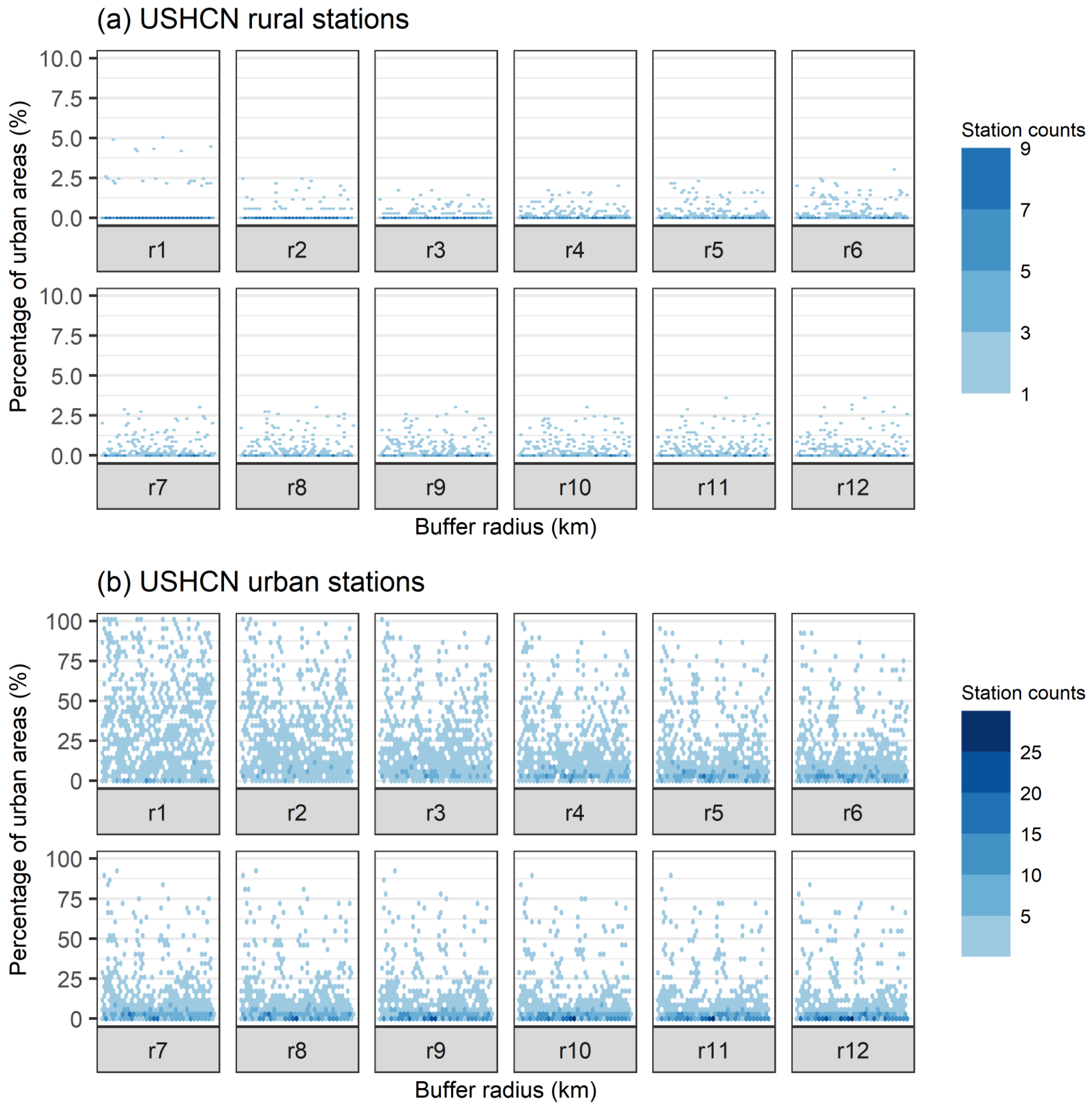
The urban area percentages around the rural and urban stations for the 1–12 km buffer radius are shown in Figure 1. The urban land percentage around the rural stations classified by machine learning is mostly less than 10%, which well fits the definition of a rural station [11,39]. Therefore, it is reasonable to choose 0.2 as the contamination parameter of the model and to select the rural stations.
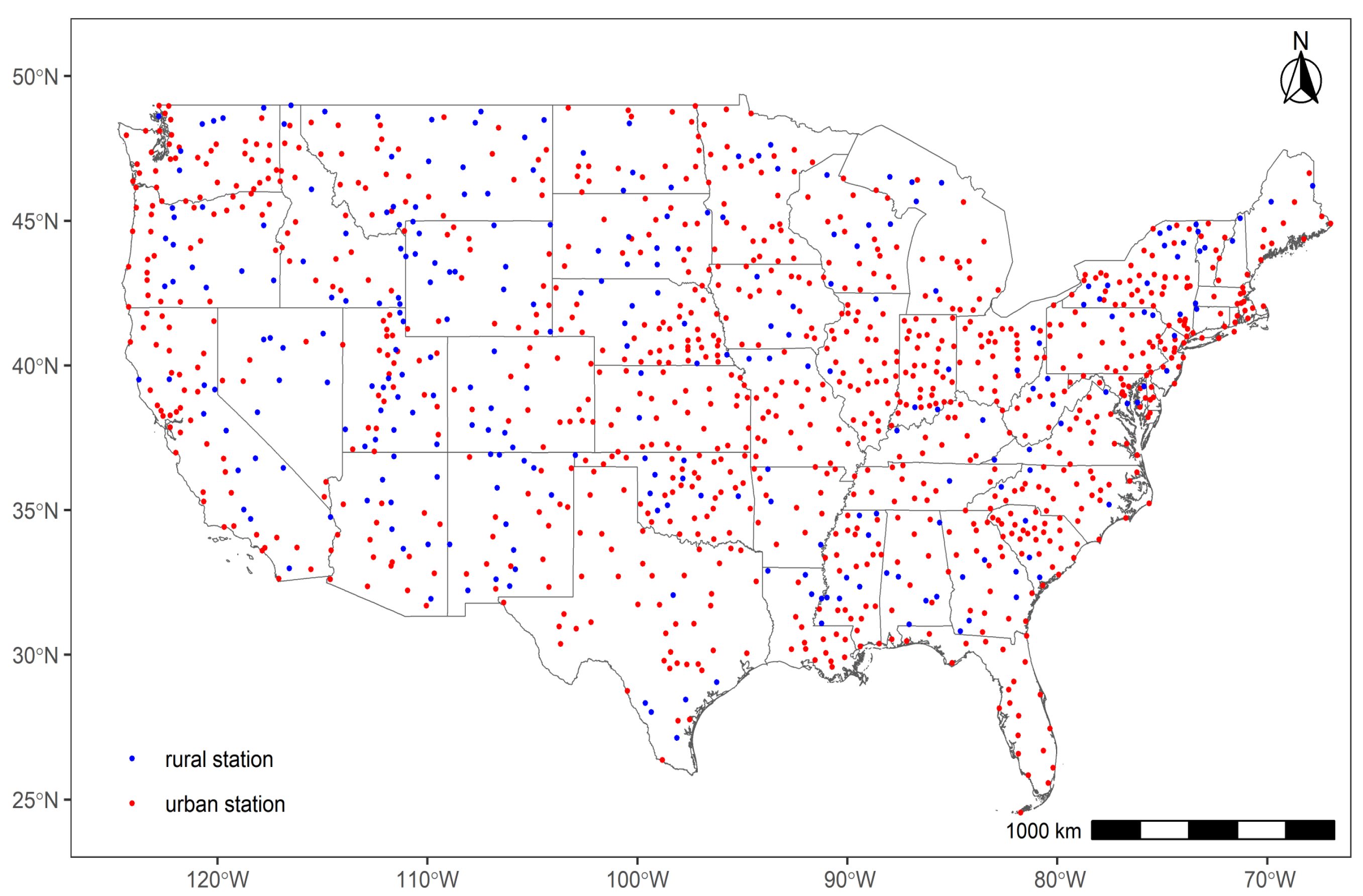
The spatial distribution of the USHCN rural stations and urban stations selected by the machine learning method are shown in Figure 2. In the plain regions, the rural stations are relatively sparser due to the more rapid urbanization, but they generally have an even distribution across the study area and can guarantee the overall comparison of the SAT change between all stations and rural stations.
2.2.2. Regional Average
Since the USHCN stations are not strictly evenly distributed in the contiguous United States, the regional average series cannot be calculated with a simple arithmetic average of the station series in the region. In this study, the contiguous United States was divided into a latitude–longitude grid, and the regional mean SAT series was calculated using the spatial area-weighted average method [41].
To eliminate (or attenuate) the effect of altitude in calculating regional mean time series, this research uses the temperature series anomaly ΔTi for the area-weighted average, which is more spatially conservative than when calculated with the actual temperature, and its expression is as follows:
where is the actual temperature series of the station and is the average of the time series of the reference period. In this paper, the reference period is 1961–1990, when the data of most stations are relatively complete.
The area weighted average was calculated based on the method used in Jones et al. (1996) [41] and Ren et al. (2023) [42], which applied the cosine value of mid-latitude for each of the latitude–longitude grid cells as weights.
The specific test calculation steps in this research are as follows:
- Calculating the anomaly: The station SAT series are calculated to form SAT anomalies relative to the reference period (1961–1990).
- Gridding: Due to the high density of USHCN stations and the regional scale of climate in the contiguous United States, as well as for the convenience of comparison with previous relevant studies, the research area is divided into a 2° × 2° latitude–longitude grid [43,44], and the mean temperature anomalies of all stations in each grid cell are calculated every year to obtain the temperature anomaly series of each grid cell.
- Regional average: The spatial area-weighted average method is adopted for the calculation, with the cosine of each grid cell’s latitude (the mid-latitude value) used as the weight to obtain the regional average temperature anomalies of the whole research area.
2.2.3. Evaluation Method of Urbanization Effect
The urbanization effects on the estimation of extreme and mean temperature trends in the contiguous United States were evaluated based on monthly mean maximum surface air temperature (Tmax), monthly mean minimum surface air temperature (Tmin), and monthly mean surface air temperature (Tmean) of the USHCN stations.
In order to ensure the integrity of the temperature series to obtain a more accurate estimate of temperature trends and urbanization effects, only the grid cells with at least 80% valid data during the total study period (1921–2020) were selected for use in the study.
Urbanization effects refer to the impacts of urbanization on trends in temperature series of observation stations in or nearby urban areas. Studies have shown that the development of cities is random, and the urbanization effect is not linear in a short period of time [45,46]. In long-term climate change studies, however, the main focus is on long-term temperature trends, and the short-term nonlinear fluctuations can be ignored. Therefore, the urbanization effect is defined here as the linear trend of temperature difference series of all stations and rural stations in the grid cell or study area [47]; its calculation formula is as follows:
where Tall is the trend of temperature anomaly series at all stations in the grid, Trural is the trend of temperature anomaly series at rural stations in this grid cell, is the trend difference of the Tall and Trural, or the trend of difference series between Tall and Trural in the grid cell or whole study region. The unit of urbanization effect is °C per decade (°C dec−1).
The urbanization contribution (Uc) refers to the percentage of urbanization effect to the overall temperature trend of all stations in the grid cell or study region [47], and its calculation formula is as follows:
3. Results
3.1. Overall Temperature Trend
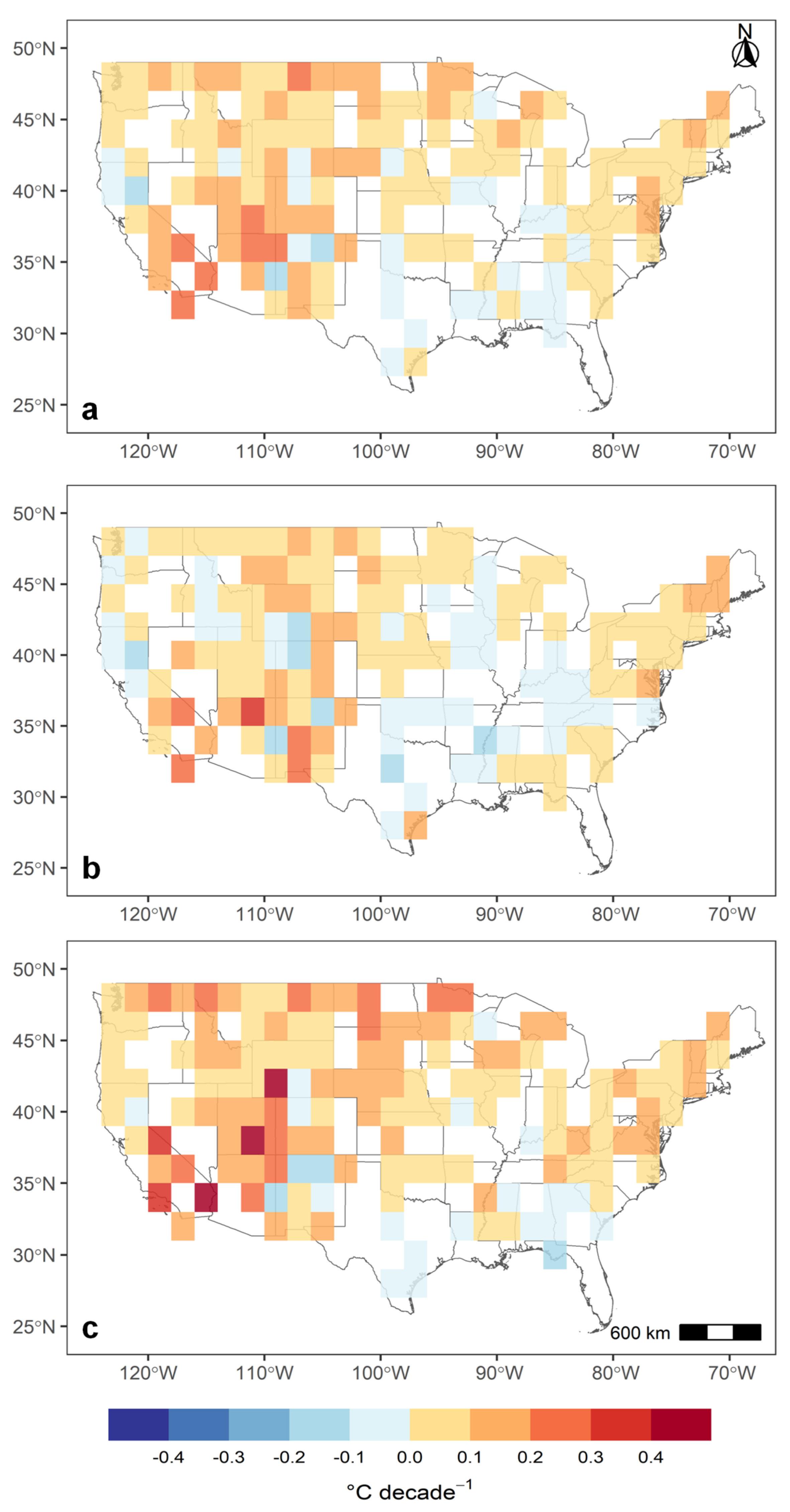
The SAT of the USHCN stations in the contiguous United States has increased significantly since 1921. The distributions of the overall trend of annual mean Tmax, Tmin, and Tmean of all stations in each grid cell are shown in Figure 3. For the annual mean SAT, the annual mean trend in most grid cells is positive, and it generally ranges from −0.1 to 0.3 °C dec−1. The annual mean Tmax trends are generally between −0.1 and 0.2 °C dec−1, and the annual mean Tmin shows a spatially more consistent warming across the study region, with the trends generally between −0.2 and 0.3 °C dec−1. The Tmin in the eastern coast and the whole western region increased more significantly, while in the southern Gulf Coast it shows a slight cooling trend.
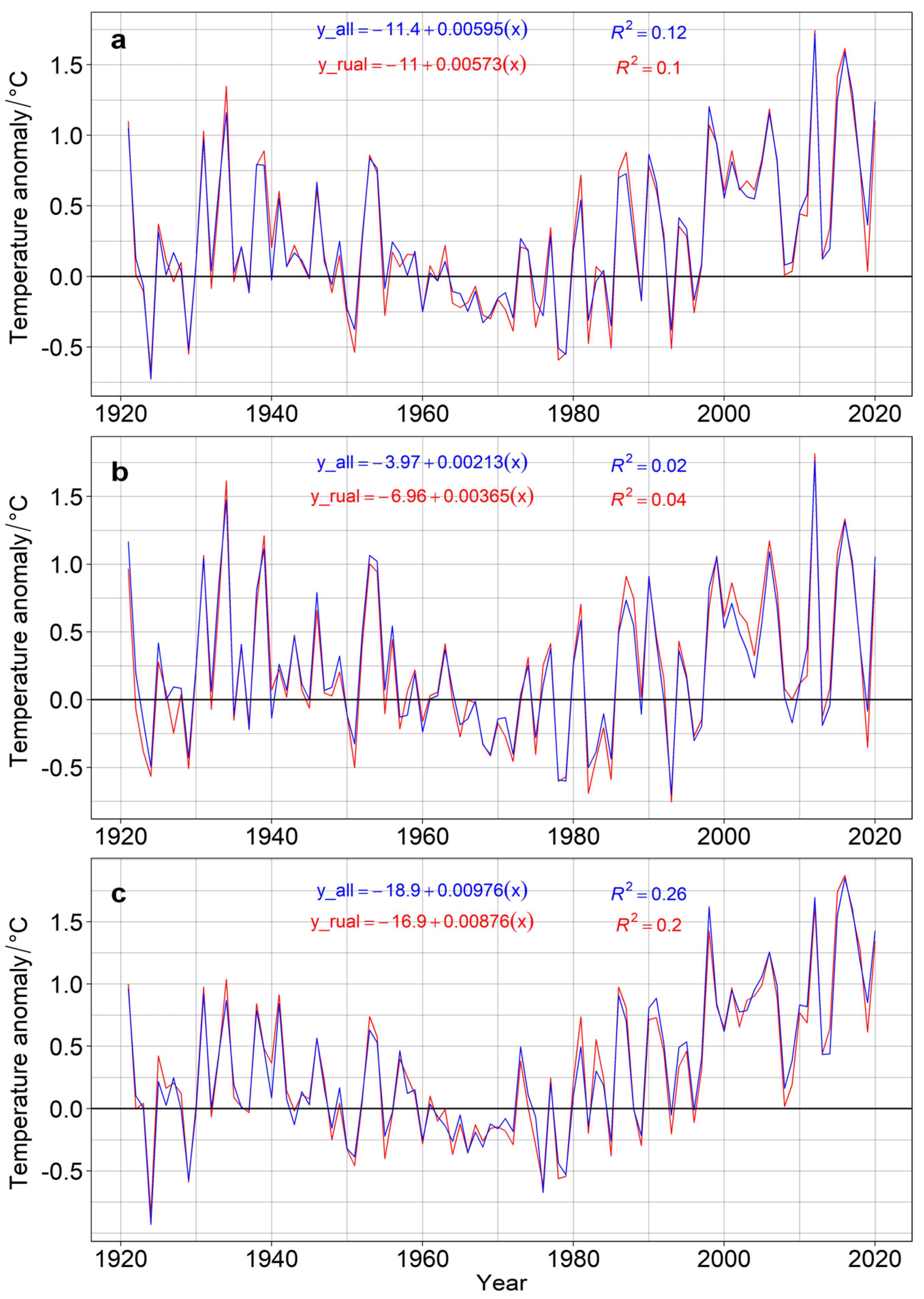
Figure 4 shows the regional annual mean temperature anomaly series for all stations and rural stations. The annual mean SAT trend of the study region in the last hundred years is 0.059 °C dec−1, and the trends of the annual mean Tmax and Tmin in the whole region are 0.022 °C dec−1 and 0.097 °C dec−1, respectively. The inter-annual to decadal variability in SAT at all stations and rural stations are similar and the positive trends in Tmean and Tmin are significant statistically. Although the SAT anomaly differences between the two types of stations are not intuitively visible, but the upward trends of all stations are slightly higher than those of the rural stations for Tmean and Tmin, indicating a possible urbanization effect in the SAT data series of the all stations.
3.2. Urbanization Effect
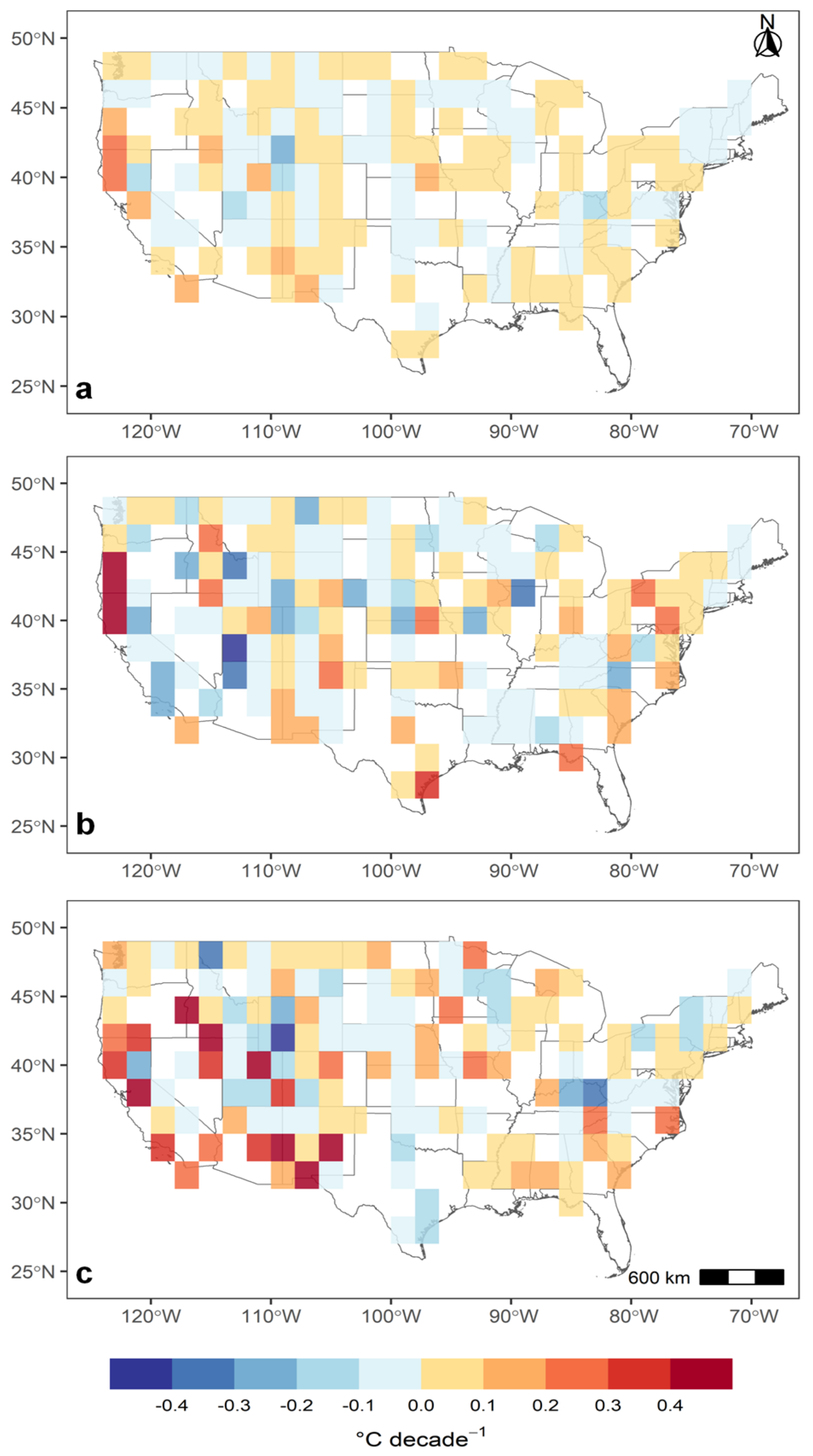
After selecting the research grid cells according to the above criteria, the time series of the Tmax, Tmin, and Tmean anomalies of all stations and rural stations in each grid cell were arithmetically averaged, and the mean anomaly series of each grid was obtained. According to Formula (2), the urbanization effect of the temperature indices on each grid cell were calculated, and their distributions are shown in Figure 5.
Figure 5a shows that the urbanization effects of the annual mean temperature series in the contiguous United States in the last hundred years are mostly distributed in the range of −0.1~0.2 °C dec−1. The urbanization effect is generally greater in the western areas, but there is no spatially consistent pattern of the positive or negative urbanization effects across the whole contiguous United States.
For the Tmax series, the urbanization effects are mostly distributed in the range of −0.2~0.1 °C dec−1 (Figure 5b), indicating more grid cells with a negative urbanization effect in the Tmax data series of the USHCN. In the eastern, central, and western coastal regions, the Tmax series contains larger positive urbanization effects. In the southern United States near the Gulf of Mexico, there are more grid cells with negative urbanization effects, which may be due to the fact that coastal urban stations are affected by the ocean, and the Tmax responds relatively slowly to the urbanization signal [46]. Some grid cells in the central and western regions also show negative urbanization effects.
In some areas, urbanization leads to an increase in aerosol emissions, which results in a decrease in solar radiation on the surface of the Earth and a small decrease in SAT during the daytime. Especially in the eastern part of the United States, urban pollution is more serious, with aerosol concentrations in urban areas being higher than those in rural areas, and Tmax increases more slowly than that in rural stations, which may have resulted in a negative urbanization effect of Tmax [46]. In addition, in the arid area of central and western regions, as well as the difference in vegetation cover and irrigation between urban and rural areas, may also lead to the negative urbanization effect; that is, the greening and irrigation of urban areas are more than that of rural areas, which makes the Tmax of urban areas in summer rise slower than the surrounding desert areas, thus leading to the negative urbanization effect of Tmax [48,49].
Compared to the Tmax, the urbanization effect on the Tmin trends is more positive and more significant (Figure 5c). The urbanization effects in the last hundred years are mostly distributed in the range of −0.1~0.2 °C dec−1. Larger positive urbanization effects are observed in the northwest and western coastal regions and the southeastern Gulf of Mexico, while the urbanization effect on some grid cells is negative in the central plains and northeastern parts of the study region.
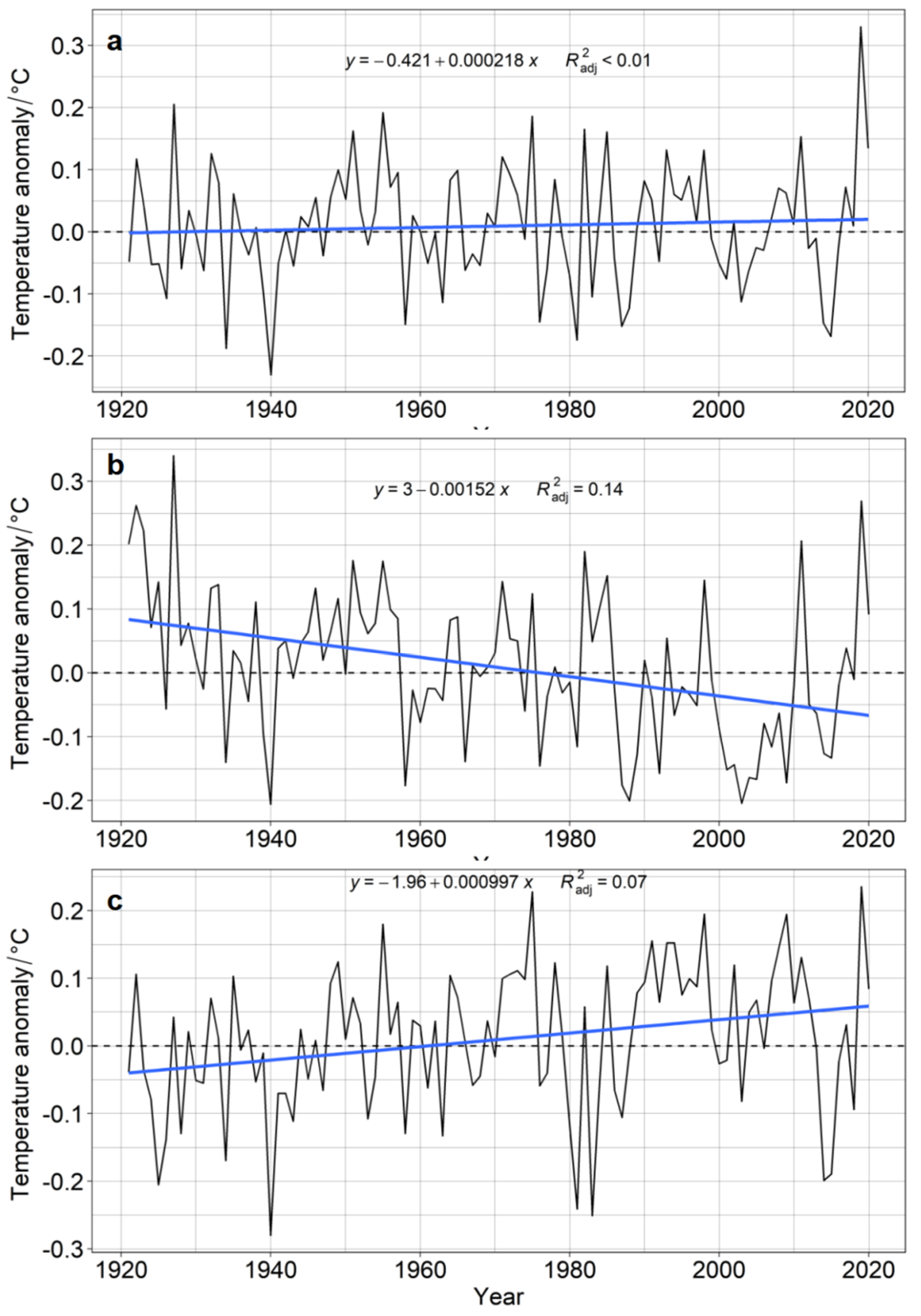
Figure 6 shows the SAT difference series of the regional mean time series between all stations and rural stations, and their trends or urbanization effects for Tmean, Tmax, and Tmin. The difference series of Tmean and Tmin showed a positive trend; urbanization had warming effect on Tmean and Tmin. However, the difference series of Tmax showed a negative trend, with urbanization having a cooling effect on Tmax of the contiguous United States in the last century.
The region-averaged urbanization effect in the annual mean temperature series in the contiguous United States is estimated to be 0.002 °C dec−1 (p < 0.1), and the region-averaged urbanization effects in the Tmax and Tmin temperature series in the study region are −0.015 °C dec−1 (p < 0.05) and 0.013 °C dec−1 (p < 0.05), respectively.
3.3. Urbanization Contribution
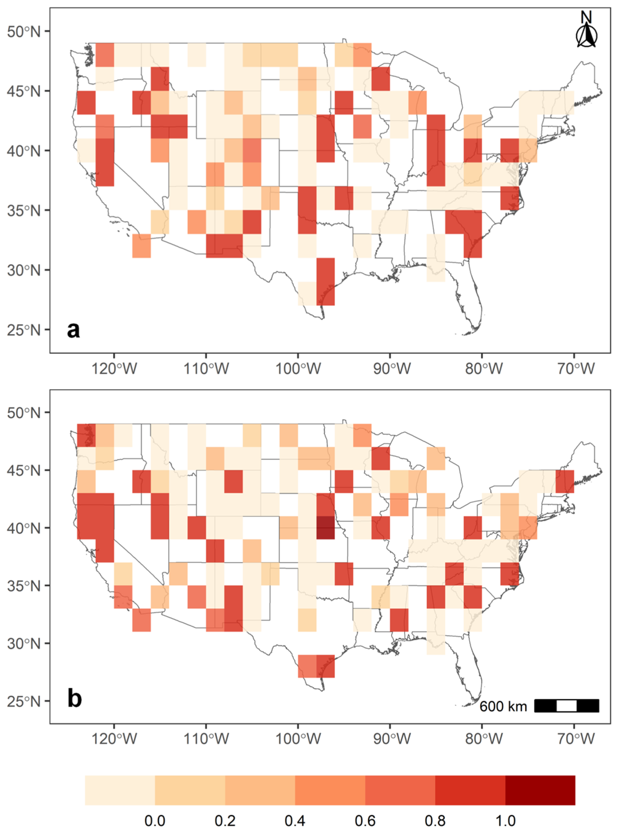
According to Formula (3), the annual mean urbanization contribution in each grid cell and in the contiguous United States on the whole were calculated, and their distribution is shown in Figure 7. The region-averaged annual mean SAT urbanization contribution is estimated to be 35%, despite the region-averaged annual mean urbanization effect being only marginally significant. The urbanization contribution for the annual mean Tmin in the whole region is 34%. However, urbanization has caused a cooling change in the annual mean Tmax in the study region on the whole, while the overall trend in annual mean Tmax is positive. In this case, the urbanization contribution was not calculated and shown.
The results show that, although the homogenization method in Menne et al. (2009) [34] may have produced the urban blending effect, leading to the non-representativeness in the selected rural stations, there is still an urbanization bias to a certain extent in the existing USHCN homogenized data set. The urbanization around the USHCN stations has led to at least one-third of the overall warming in terms of the annual mean SAT change, as recorded at USHCN stations over the last one hundred years.
As shown in Figure 7a, the urbanization contribution to the annual mean temperature trend is relatively small in the central region, while it is larger in the eastern and western coastal areas. In addition, larger urbanization contribution can also be observed in the central plain region. From Figure 7b, a larger urbanization contribution for the annual mean Tmin can be observed in the western and northeastern contiguous United States, while the central and southern plains see a relatively small value.
The results of the study for each temperature index mentioned above are summarized in Table 1.
4. Discussion
The above results show that urbanization has a certain impact on the surface air temperature series in the contiguous United States in the last hundred years, but the magnitude of the urbanization effect differs among SAT indices and regions. The urbanization effect in the Tmin series is larger than that in the Tmean series. However, in contrast to previous studies, the research object of this paper was the USHCN-v2.5-TOB data set as a whole instead of each USHCN station; for our research method, this study introduced a machine learning method to select rural stations, with a more objective, comprehensive and diversified consideration of the local environment around the stations [26]. In addition, it is worth noting that, in this study, the current land use data around the stations were only taken as a reference to divide urban and rural stations and quantify the urbanization level around each station. Although land use change is one of the major factors causing urbanization effects, the physical relationship between land use change and SAT change has not been analyzed. This needs to be examined in combination with other methods in the future.
4.1. Comparison with Other Relevant Studies
Similar to the conclusions of this study, previous studies have shown that, since the early 20th century, urbanization bias in the historical SAT data series of the United States has been roughly in the range of 0.04~0.06 °C dec−1, and the contribution of urbanization is around 20% [22,24,25,26]. However, there are also some studies indicating that the urbanization effect on SAT trends in the United States is not significant and may only account for 5% of the total SAT increase in the last hundred years (e.g., Karl et al. (1988); Hansen et al. (2010)) [2,27,28,29,30]. The data and methods used and the study areas of the above-mentioned studies are different, so the obtained results are also different and cannot be strictly comparable. However, the largest potential factor influencing the results is the method used to select rural stations.
The division of urban and rural stations in previous studies is mostly based on individual indicators such as satellite nightlights, impermeable surfaces, and population growth [4,27]; the selection standards are relatively subjective, and there is a lack of diversified and comprehensive consideration of the climatic environments around the stations. However, the machine learning based station selection method used in this study mainly divides urban and rural stations according to the percentage of urban land use in the buffer zone of 1–12 km radius around the station, and has a more precise and detailed consideration of the surrounding environment of each station. It can produce a more representative reference data series of stations and can be used to more objectively assess the urbanization effect in the regional SAT data series. This is the reason that a larger urbanization effect has been detected in this study in the homogenized USHCN data, although the urban blending effect may have existed in the process of data homogenization [34].
In future studies, the urbanization degree of each station can be defined according to the percentage of urban land use at different buffer radii, and the relationship between urbanization degree (or urban size) and urbanization bias can be examined. In addition, different from previous studies, this study made full use of USCRN network data, and made use of the high representativeness of the CRN stations in rural climate environment to re-classifies USHCN stations into urban and rural stations. This not only provides a new theoretical and methodological basis for the identification and classification of urban and rural stations in future relevant research, but also provides a favorable reference for the construction and planning of reference climate station networks in other regions.
On the whole, the new findings reported in this study can help deepen our understanding of the biases in the homogenized USHCN SAT data. This will be helpful for future regional climate change monitoring, climate model evaluation, climate policy formulation, and the construction of national reference climate station networks.
4.2. Limitations of the Study
4.2.1. Limitations of Research Methods
In terms of station selection, the machine learning methods used in this study still have room for improvement. In the machine learning model constructed in this study, the determination of the contamination parameter can still be improved. As mentioned in the Research Methods section, the surrounding environments of some CRN stations changed since the establishment of the stations. Although this number is small, the urban land area around some CRN stations still accounts for more than 10%, indicating that the training data set itself was affected by urbanization to a certain extent. However, it is difficult to determine the proportion and extent of the urbanization effect of CRN stations, which often needs to be estimated by referring to other relevant studies and research experience. In this study, 0.2 was selected as the model contamination parameter. The urban land percentage around the rural stations is mostly less than 10%, meeting the criteria for rural stations [11], and the distribution of rural stations is relatively uniform, so the selection of this contamination parameter is reasonable, although the urbanization bias assessment results in this research should be relatively conservative, due to this compromise, to determine the contamination parameter and to select the rural stations.
In terms of SAT trend estimation, the methods used in this study still have room for improvement. Studies have shown that the urbanization effect is not linear in a period of time, because the influence of landscape alterations is non-linear [50,51]. However, most of the urbanization bias assessment methods widely used at present treat the urbanization effect as a linear trend and correct the systematic bias in SAT series by evenly allocating the cumulative urbanization effect to each year of the data series. Therefore, there are still uncertainties in the current assessment methods. In view of these problems, future studies will consider combining new statistical models and methods, including spatiotemporal weighted regression method, to conduct more detailed assessment of urbanization effects and improve the results of urbanization bias assessment. In addition, the synergic influence of land use, population, aerosol emission, natural variability of climate and other factors on UHI and the urbanization bias will be examined by combining various data sets, so as to establish more accurate historical air temperature data series.
4.2.2. Uncertainty of Research Data
In addition, the USHCN-v2.5 data set used in this paper was homogenized, and the pairwise homogenization algorithm (PHA) method used in the homogenization process may have yielded an urban blending effect [34]; that is, the urbanization bias in the temperature series of urban stations was weakened, while that of rural stations was strengthened to a certain extent, which also resulted in relatively small urbanization effects in the assessment results, as compared to those reported in China (e.g., Yang et al., 2011; He et al., 2023) [18,52]. A possible reason for the urban blending effect is that during the process of homogenization, the selected reference stations included both urban and rural stations, and the trend was revised to a certain extent when revising the break point in the series; in other words, the higher temperature trend of an urban station was reduced to be consistent with that of the rural reference station, and the smaller warming trend of a rural reference station was adjusted to be consistent with that of the urban target station. This would result in a temperature trend of the urban and rural stations that eventually tends to close an average value. In this case, the urbanization effect in the homogenized data series was weakened to a certain extent [52]. Therefore, the real urbanization effect in the USHCN data set would be larger if the SAT trends at the rural stations had not been increased due to the urban blending effect in the data homogenization process. However, our analysis shows that on the whole, the USHCN-v2.5 data still overestimate large-scale regional warming to some extent. This is meaningful for future climate change research and assessment, which helps us realize the uncertainties in estimating climate trends in the USHCN data, and can provide a data analysis reference for future climate model assessment and large-scale climate change monitoring. The IPCC’s lower estimate of urbanization bias in the global temperature data based on homogenized temperature records may have been caused by the urban blending effect [21].
Since the main purpose of this study was to evaluate the systematic bias of urbanization in the currently applied USHCN data set, the rationality of the homogenization method was not considered here. However, the possible urban blending effect on trends of rural stations in the data homogenization process may have led to further underestimations of urbanization effects in the latest homogenized USHCN data series. These issues need to be investigated in future research.
In future studies, urbanization effect assessment can be performed using different homogenized USHCN data, including the original SAT data. Facilitated comparisons with relevant studies in China and other regions are also needed. In terms of methods, when screening stations and grid points, there are still blank grid cells or missing data in some areas. There is a need to adjust the station screening criteria, or to combine other station screening methods to obtain a more ideal spatial distribution of stations.
5. Conclusions
In this study, we used a machine learning method (the “isolated forest” algorithm) to select rural stations from the USHCN stations and assessed urbanization effects on the Tmax, Tmin and Tmean series of all the USHCN stations in the last hundred years. The following conclusions were drawn:
- Since 1921, the urbanization effects in the latest homogenized Tmean, Tmax, and Tmin data series in the contiguous United States are 0.002 °C dec−1, −0.015 °C dec−1 and 0.013 °C dec−1, respectively, and the urbanization contributions are 35% and 34% for Tmean and Tmin, respectively.
- The urbanization effects are roughly distributed within −0.1~0.2 °C dec−1 for the annual mean Tmean, with about half of the grid cells showing an urbanization warming effect. Urbanization effects are distributed within −0.2~0.3 °C dec−1 for the annual mean Tmin series, and they are positive in most regions, with positive urbanization effects that are most extensive in the northwestern, western and southeastern coastal areas.
- For Tmean, Tmax and Tmin, the urbanization effects in the eastern and western coastal areas of the United States are generally more significant. However, there are also some grid cells with negative urbanization effects, among which the negative effect of Tmax is the most significant.
There are uncertainties in the conclusions of this study. They may be caused by the urban blending effect due to the data homogenization method used, the uneven distribution of stations and grid cells due to the station selection criteria, and the relatively subjective method of selecting contamination parameters for the machine learning model. In spite of these uncertainties, the analysis results can help us in understanding systematic bias of SAT data in the United States and provide a basis for further adjustments of the data for use in climate change monitoring and detection.
Author Contributions
S.H. wrote the original draft; G.R. and P.Z. reviewed and edited the manuscript; G.R., S.H. and P.Z. developed the methodology; supervision, project administration and funding acquisition by G.R. All authors have read and agreed to the published version of the manuscript.
Funding
This study is supported by the National Key R&D Program of China (2018YFA0605603).
Data Availability Statement
The data that support the findings of this study are available in national centers for environmental information. These data were derived from the following resources: the U.S. Historical Climatology Network and the U.S. Climate Reference Network, with reference numbers DOI: https://doi.org/10.1175/2008BAMS2613.1 and DOI: https://doi.org/10.1175/BAMS-D-12-00170.1, respectively (accessed on 13 March 2024).
Acknowledgments
The U.S. Climate Reference Network (CRN) data set was provided by the National Oceanic and Atmospheric Administration (NOAA). The global land use/land cover data set was provided by the ESA CCI Land Cover Project (“www.esa-landcover-cci.org (accessed on 16 March 2024)”).
Conflicts of Interest
The authors declare no conflicts of interest.
References
- Arias, P.A.; Bellouin, N.; Coppola, E.; Jones, R.G.; Krinner, G.; Marotzke, J.; Naik, V.; Palmer, M.D.; Plattner, G.K.; Rogelj, J.; et al. Technical Summary. In Climate Change 2021: The Physical Science Basis; Contribution of Working Group I to the Sixth Assessment Report of the Intergovernmental Panel on Climate Change; Masson-Delmotte, V., Zhai, P., Pirani, A., Connors, S.L., Péan, C., Berger, S., Caud, N., Chen, Y., Goldfarb, L., Gomis, M.I., et al., Eds.; Cambridge University Press: Cambridge, UK; New York, NY, USA, 2021; pp. 33–144. [Google Scholar]
- Karl, T.R.; Diaz, H.F.; Kukla, G. Urbanization: Its detection and effect in the United States climate record. J. Clim. 1988, 1, 1099–1123. [Google Scholar] [CrossRef]
- Fujibe, F. Detection of urban warming in recent temperature trends in Japan. Int. J. Climatol. 2009, 29, 1811–1822. [Google Scholar] [CrossRef]
- Hausfather, Z.; Menne, M.; Williams, C.; Masters, T.; Broberg, R.; Jones, D. Quantifying the impact of urbanization on U.S. Historical Climatology Network temperature records. J. Geophys. Res. Atmos. 2013, 118, 481–494. [Google Scholar] [CrossRef]
- Zhou, L.M.; Dickinson, R.E.; Tian, Y.H. Evidence for a significant urbanization effect on climate in China. Proc. Natl. Acad. Sci. USA 2004, 101, 9540–9544. [Google Scholar] [CrossRef] [PubMed]
- Luo, M.; Lau, N.C. Increasing heat stress in urban areas of eastern China: Acceleration by urbanization. Geophys. Res. Lett. 2018, 45, 13060–13069. [Google Scholar] [CrossRef]
- Andrew, G.; John, D. Trends in extreme apparent temperatures over the United States, 1949–2010. J. Appl. Meteorol. Climatol. 2011, 50, 1650–1653. [Google Scholar]
- Arthur, T.; Robert, J. Trends in twentieth-century temperature extremes across the United States. J. Clim. 2002, 15, 3188–3205. [Google Scholar]
- Evan, M.; Richard, B. A trend analysis of the 1930–2010 extreme heat events in the Continental United States. J. Appl. Meteorol. Climatol. 2014, 53, 565–582. [Google Scholar]
- Du, J.; Wang, K.; Cui, B.; Jiang, S. Correction of inhomogeneities in observed land surface temperatures over China. Atmos. Res. 2020, 33, 8885–8902. [Google Scholar] [CrossRef]
- Tysa, S.; Ren, G.; Qin, Y.; Zhang, P.; Ren, Y.; Jia, W.; Wen, K. Urbanization Effect in Regional Temperature Series Based on a Remote Sensing Classification Scheme of Stations. J. Geophys. Res. 2019, 124, 10646–10661. [Google Scholar] [CrossRef]
- Gong, D.; Wang, S. Uncertainty in global warming research. Earth Sci. Front. 2002, 9, 371–376. (In Chinese) [Google Scholar]
- Zhao, Z.C. The changes of temperature and the effects of the urbanization in China in the last 39 years. Meteor. Monogr. 1991, 17, 14–16. (In Chinese) [Google Scholar]
- Shi, Z.T.; Jia, G.S.; Hu, Y.H.; Zhou, Y.Y. The contribution of intensified urbanization effects on surface warming trends in China. Theor. Appl. Climatol. 2019, 138, 1125–1137. [Google Scholar] [CrossRef]
- Shi, T.; Yang, Y.J.; Sun, D.B.; Huang, Y.; Shi, C. Influence of Changes in Meteorological Observational Environment on Urbanization Bias in Surface Air Temperature: A Review. Front. Clim. 2022, 3, 781999. [Google Scholar] [CrossRef]
- Mahmood, R.; Foster, S.A.; Logan, D. The Geoprofille metadata, exposure of instruments, and measurement bias in climatic record revisited. Int. J. Clim. 2006, 26, 1091–1124. [Google Scholar] [CrossRef]
- Cao, L.; Zhu, Y.; Tang, G.; Yuan, F.; Yan, Z. Climatic warming in China according to a homogenized data set from 2419 stations. Int. J. Climatol. 2016, 36, 4384–4392. [Google Scholar] [CrossRef]
- Yang, X.; Hou, Y.; Chen, B. Observed surface warming induced by urbanization in east China. J. Geophys. Res. 2011, 116, D14113. [Google Scholar] [CrossRef]
- Das, L.; Annan, J.D.; Hargreaves, J.C.; Emori, S. Centennial scale warming over Japan: Are the rural stations really rural? Atmos. Sci. Lett. 2011, 12, 362–367. [Google Scholar] [CrossRef]
- Connolly, R.; Connolly, M. Has poor station quality biased U.S. temperature estimates? Open Peer Rev. J. 2014, 11. Available online: http://oprj.net/articles/climate-science/11 (accessed on 8 December 2021).
- Yang, X.; Leung, L.R.; Zhao, N.; Zhao, C.; Yun, Q.K.H.; Liu Chen, B. Contribution of urbanization to the increase of extreme heat events in an urban agglomeration in east China. Geophys. Res. Lett. 2017, 44, 6940–6950. [Google Scholar] [CrossRef]
- Genki, K.; Ronan, C.; Peter, O. Evidence of Urban Blending in Homogenized Temperature Records in Japan and in the United States: Implications for the Reliability of Global Land Surface Air Temperature Data. J. Appl. Meteorol. Climatol. 2023, 62, 1095–1114. [Google Scholar]
- Ma, X.B. A review of the urbanization process in the United States and its experience. J. Guizhou Univ. Soc. Sci. 2019, 37, 40–46. (In Chinese) [Google Scholar]
- Connolly, R.; Connolly, M. Urbanization bias III. Estimating the extent of bias in the Historical Climatology Network datasets. Open Peer Rev. J. 2014, 34, ver. 0.1. [Google Scholar]
- Scafetta, N. Detection of non-climatic biases in land surface temperature records by comparing climatic data and their model simulations. Clim. Dyn. 2021, 56, 2959–2982. [Google Scholar] [CrossRef]
- Zhang, P.; Ren, G.; Qin, Y.; Zhai, Y.; Zhai, T.; Tysa, S.; Xue, X.; Yang, G.; Sun, X. Urbanization effects on estimates of global trends in mean and extreme air temperature. J. Clim. 2021, 34, 1923–1945. [Google Scholar] [CrossRef]
- Hansen, J.; Ruedy, R.; Sato, M.; Lo, K. Global surface temperature change. Rev. Geophys. 2010, 48, RG4004. [Google Scholar] [CrossRef]
- Parker, D.E. A demonstration that large-scale warming is not urban. J. Clim. 2006, 19, 4179–4197. [Google Scholar] [CrossRef]
- Jones, P.D.; Lister, D.H.; Li, Q. Urbanization effects in largescale temperature records, with an emphasis on China. J. Geophys. Res. 2008, 113, D16122. [Google Scholar] [CrossRef]
- Hausfather, Z.; Cowtan, K.; Menne, M.; Williams, C.N., Jr. Evaluating the impact of U.S. Historical Climatology Network homogenization using the U.S. Climate Reference Network. Geophys. Res. Lett. 2016, 43, 1695–1701. [Google Scholar] [CrossRef]
- Oke, T. The energetic basis of the urban heat island. Q. J. R. Meteor. Soc. 1982, 108, 1–24. [Google Scholar] [CrossRef]
- Diamond, H.; Karl, T.; Palecki, M.; Baker, C.; Bell, J.; Leeper, R.; Easterling, D.; Lawrimore, J.; Meyers, T.; Helfert, M.; et al. Climate reference network after one decade of operations: Status and assessment. Bull. Am. Meteorol. Soc. 2013, 94, 485–498. [Google Scholar] [CrossRef]
- Ren, G.; Chu, Z. Construction of American climate reference network and its enlightenment. China Meteorol. Adm. 2019, 9, 56–61. (In Chinese) [Google Scholar]
- Menne, M.; Williams, C.N., Jr.; Vose, R. The U.S. Historical Climatology Network monthly temperature data, version 2. Bull. Amer. Meteor. Soc. 2009, 90, 993–1007. [Google Scholar] [CrossRef]
- Hollmann, R.; Merchant, C.J.; Saunders, R.; Downy, C.; Buchwitz, M.; Cazenave, A.; Chuvieco, E.; Defourny, P.; de Leeuw, G.; Forsberg, R.; et al. The ESA climate change initiative: Satellite data records for essential climate variables. Bull. Amer. Meteor. Soc. 2013, 94, 1541–1552. [Google Scholar] [CrossRef]
- Khan, S.; Madden, M. A survey of recent trends in one class classification. In Artificial Intelligence and Cognitive Science. AICS 2009. Lecture Notes in Computer Science, vol 6206; Coyle, L., Freyne, J., Eds.; Springer: Berlin/Heidelberg, Germany, 2010; pp. 188–197. [Google Scholar]
- Liu, F.; Ting, K.; Zhou, Z. Isolation Forest. In Proceedings of the 2008 Eighth IEEE International Conference on Data Mining (ICDM), Pisa, Italy, 15–19 December 2008; pp. 413–422. [Google Scholar]
- Liu, F.; Ting, K.; Zhou, Z. Isolation-based anomaly detection. ACM Trans. Knowl. Discov. Data 2012, 6, 1–39. [Google Scholar] [CrossRef]
- Ren, G. Urbanization as a major driver of urban climate change. Adv. Clim. Chang. Res. 2015, 6, 1–6. [Google Scholar] [CrossRef]
- Li, Y.; Wang, L.; Zhou, H.; Zhao, G.; Ling, F.; Li, X.; Qiu, J. Urbanization effects on changes in the observed air temperatures during 1977–2014 in China. Int. J. Climatol. 2018, 39, 251–265. [Google Scholar] [CrossRef]
- Jones, P.D.; Hulme, M. Calculating regional climatic time series for temperature and precipitation: Methods and illustrations. Int. J. Climatol. 1996, 16, 361–377. [Google Scholar] [CrossRef]
- Ren, G.; Wang, G.; Li, Q. Principles of Climate Change Monitoring and Detection Technology, 1st ed.; China Meteorological Press: Beijing, China, 2023; pp. 214–228. [Google Scholar]
- Dunn, L.; Donat, M.; Alexander, L. Investigating uncertainties in global gridded data sets of climate extremes. Clim. Past 2014, 10, 2171–2199. [Google Scholar] [CrossRef]
- Avila, F.; Dong, S.; Menang, K.; Rajczak, J.; Renom, M.; Donat, M.; Alexander, L. Systematic investigation of gridding-related scaling effects on annual statistics of daily temperature and precipitation maxima: A case study for south-east Australia. Weather. Clim. Extrem. 2015, 9, 6–16. [Google Scholar] [CrossRef]
- Oke, T.R. City size and the urban heat island. Atmos. Environ. 1973, 7, 769–779. [Google Scholar] [CrossRef]
- Yang, Y.; Guo, M.; Wang, L.; Zong, L.; Liu, D.; Zhang, W.; Wang, M.; Wan, B.; Guo, Y. Unevenly spatiotemporal distribution of urban excess warming in coastal Shanghai megacity, China: Roles of geophysical environment, ventilation and sea breezes. Build. Environ. 2023, 235, 110180. [Google Scholar] [CrossRef]
- Ren, G.; Zhou, Y. Urbanization effect on trends of extreme temperature indices of national stations over mainland China, 1961–2008. J. Clim. 2014, 27, 2340–2360. [Google Scholar] [CrossRef]
- Xue, J.; Zong, L.; Yang, Y.; Bi, X.; Zhang, Y.; Zhao, M. Diurnal and interannual variations of canopy urban heat island (CUHI) effectsover a mountain-valley city with a semi-arid climate. Urban Clim. 2023, 48, 101425. [Google Scholar] [CrossRef]
- Dong, Z.; Wang, L.; Xu, P.; Cao, J.; Yang, R. Heatwaves similar to the unprecedented one in summer 2021 over western North America are projected to become more frequent in a warmer world. Earth’s Future 2023, 11, e2022EF003437. [Google Scholar] [CrossRef]
- Elvidge, C.; Tuttle, B.; Sutton, P.; Baugh, K.; Howard, A.; Milesi, C.; Bhaduri, B.; Nemani, R. Global distribution and density of constructed impervious surfaces. Sensors 2007, 7, 1962–1979. [Google Scholar] [CrossRef] [PubMed]
- Peterson, T.; Owen, T. Urban heat island assessment: Metadata are important. J. Clim. 2005, 18, 2637–2646. [Google Scholar] [CrossRef]
- He, J.; Ren, G.; Zhang, P.; Zheng, X.; Zhang, S. Updated analysis of surface warming trends in North China based on in-depth homogenized data (1951−2020). Clim. Res. 2023, 91, 47–66. [Google Scholar] [CrossRef]
Figure 1.
Percentages of urban land of (a) USHCN rural stations and (b) USHCN urban stations at buffer radii of 1–12 km. r1-r12 on the X-axis label refer to buffer radii of 1-12km around the stations respectively.
Figure 1.
Percentages of urban land of (a) USHCN rural stations and (b) USHCN urban stations at buffer radii of 1–12 km. r1-r12 on the X-axis label refer to buffer radii of 1-12km around the stations respectively.

Figure 2.
Distribution of the selected USHCN urban stations (red) and rural stations (blue) when the contamination parameter is set as 0.2.
Figure 2.
Distribution of the selected USHCN urban stations (red) and rural stations (blue) when the contamination parameter is set as 0.2.

Figure 3.
Distributions of the grid-averaged annual SAT trends for (a) mean temperature (Tmean), (b) mean maximum temperature (Tmax), and (c) mean minimum temperature (Tmin).
Figure 3.
Distributions of the grid-averaged annual SAT trends for (a) mean temperature (Tmean), (b) mean maximum temperature (Tmax), and (c) mean minimum temperature (Tmin).

Figure 4.
Regional averaged annual mean surface air temperature anomaly series of all USHCN stations (blue) and rural stations (red) for (a) Tmean, (b) Tmax, and (c) Tmin over the contiguous United States. Note that R is the correlation coefficients between temperature anomalies (y) and the serial numbers of years (x).

Figure 5.
Distributions of the urbanization effects of (a) Tmean, (b) Tmax, and (c) Tmin in the contiguous United States.
Figure 5.
Distributions of the urbanization effects of (a) Tmean, (b) Tmax, and (c) Tmin in the contiguous United States.

Figure 6.
SAT anomaly difference series between all stations and rural stations and their trends (urbanization effect, blue line) for (a) Tmean, (b) Tmax, and (c) Tmin in the contiguous United States.
Figure 6.
SAT anomaly difference series between all stations and rural stations and their trends (urbanization effect, blue line) for (a) Tmean, (b) Tmax, and (c) Tmin in the contiguous United States.

Figure 7.
Distributions of urbanization contributions for (a) Tmean and (b) Tmin. Only the grid cells where the urbanization effect of Tmean and Tmin passed the significance test (p < 0.1) are shown.
Figure 7.
Distributions of urbanization contributions for (a) Tmean and (b) Tmin. Only the grid cells where the urbanization effect of Tmean and Tmin passed the significance test (p < 0.1) are shown.


Table 1.
Urbanization effects and urbanization contributions in the 100-year time series of each temperature index in the contiguous United States.
Table 1.
Urbanization effects and urbanization contributions in the 100-year time series of each temperature index in the contiguous United States.
| Temperature Index | Urbanization Effect (°C dec−1) | Urbanization Contribution (%) | Significance p-Value |
|---|---|---|---|
| Tmean | 0.002 | 35% | 0.0514 (p < 0.1) |
| Tmax | −0.015 | \ * | 9.04 × 10⁻⁵ (p < 0.05) |
| Tmin | 0.013 | 34% | 0.0059 (p < 0.05) |
* As the urbanization effect in the Tmax series is opposite to its overall trend, and the urbanization contribution is not shown here.
Disclaimer/Publisher’s Note: The statements, opinions and data contained in all publications are solely those of the individual author(s) and contributor(s) and not of MDPI and/or the editor(s). MDPI and/or the editor(s) disclaim responsibility for any injury to people or property resulting from any ideas, methods, instructions or products referred to in the content. |
© 2024 by the authors. Licensee MDPI, Basel, Switzerland. This article is an open access article distributed under the terms and conditions of the Creative Commons Attribution (CC BY) license (https://creativecommons.org/licenses/by/4.0/).
Share and Cite
MDPI and ACS Style
Huang, S.; Ren, G.; Zhang, P. Urbanization Effects in Estimating Surface Air Temperature Trends in the Contiguous United States. Land 2024, 13, 388. https://doi.org/10.3390/land13030388
AMA Style
Huang S, Ren G, Zhang P. Urbanization Effects in Estimating Surface Air Temperature Trends in the Contiguous United States. Land. 2024; 13(3):388. https://doi.org/10.3390/land13030388
Chicago/Turabian StyleHuang, Siqi, Guoyu Ren, and Panfeng Zhang. 2024. "Urbanization Effects in Estimating Surface Air Temperature Trends in the Contiguous United States" Land 13, no. 3: 388. https://doi.org/10.3390/land13030388
Note that from the first issue of 2016, this journal uses article numbers instead of page numbers. See further details here.