
Visual Perception Optimization of Residential Landscape Spaces in Cold Regions Using Virtual Reality and Machine Learning

1
School of Architecture and Design, Harbin Institute of Technology, Harbin 150001, China
2
Key Laboratory of Cold Region Urban and Rural Human Settlement Environment Science and Technology, Ministry of Industry and Information Technology, Harbin 150001, China
*
Authors to whom correspondence should be addressed.
Land 2024, 13(3), 367; https://doi.org/10.3390/land13030367
Submission received: 24 January 2024
/
Revised: 10 March 2024
/
Accepted: 11 March 2024
/
Published: 14 March 2024
(This article belongs to the Special Issue Exploring Multisensory Landscapes: 2023 Visual Resource Stewardship Conference)
Abstract
:The visual perception of landscape spaces between residences in cold regions is important for public health. To compensate for the existing research ignoring the cold snow season’s influence, this study selected two types of outdoor landscape space environments in non-snow and snow seasons as research objects. An eye tracker combined with a semantic differential (SD) questionnaire was used to verify the feasibility of the application of virtual reality technology, screen out the gaze characteristics in the landscape space, and reveal the design factors related to landscape visual perception. In the snow season, the spatial aspect ratio (SAR), building elevation saturation (BS), and grass proportion in the field of view (GP) showed strong correlations with the landscape visual perception scores (W). In the non-snow season, in addition to the above three factors, the roof height difference (RHD), tall-tree height (TTH), and hue contrast (HC) also markedly influenced W. The effects of factors on W were revealed in immersive virtual environment (IVE) orthogonal experiments, and the genetic algorithm (GA) and k-nearest neighbor algorithm (KNN) were combined to optimize the environmental factors. The optimized threshold ranges in the non-snow season environment were SAR: 1.82–2.15, RHD: 10.81–20.09 m, BS: 48.53–61.01, TTH: 14.18–18.29 m, GP: 0.12–0.15, and HC: 18.64–26.83. In the snow season environment, the optimized threshold ranges were SAR: 2.22–2.54, BS: 68.47–82.34, and GP: 0.1–0.14.
1. Introduction
The optimal design of inter-house landscape spaces in urban residential areas is conducive to the promotion of the high-quality development of urban environments [1]. Existing studies have shown that leisure activities in landscape spaces are beneficial to physical and mental health [2,3]. People are more dependent on familiar landscape spaces in residential areas, and their activities are mostly maintained in residential landscape areas [4]. These spaces play a vital role in people’s behavioral activities and psychological recovery [5]. Many studies on public health have demonstrated that the visual perception of people exposed to different environments is significantly different [5,6,7]. Consequently, it is imperative to study the factors that affect visual perception in specific environments.
Kaplan’s attention restoration theory shows that positive environmental perceptions can provide a buffering effect between daily stressors and mental stress [8]. Several studies have indicated that changes in building roof contours, façade decorations, and building height have an impact on a user’s potential to have a restorative experience [9]. In recent years, the field of visual perception has attracted significant attention. More than 80% of information received by humans comes from the visual system [10]. The elements and attributes of a landscape environment can affect people’s psychology and physiology, and extracting and optimizing environmental factors can effectively improve health [11,12,13,14]. Researchers have conducted a significant amount of research on the effect of landscape environments on visual perception. In the research field of visual perception, most of the existing literature focuses only on the effect of light environment indicators (illuminance, daylight uniformity) on people’s visual perception and physical and mental health [15,16], but visual comfort includes not only a suitable light environment but also other visual perception factors, such as aesthetic preference. Owing to limitations in technology and equipment, research on the visual evaluation of other factors in the architectural visual environment, such as geometry, material, and color, is limited [16]. Brain responses acquire information through thoughts, experiences, and senses [17]. Environmental assessment is usually carried out by defining people’s different visual perception evaluations. Qualitative analyses in this context have typically employed research methods including questionnaires [18], self-report scales [19], group discussions, and interviews [20]. Rogge et al. used the “Likert scale” and “factor analysis” for visual evaluation to obtain users’ emotional feelings and reveal aesthetic preferences [21]. Zhang et al. investigated the correlation between street view perception and emotions among college students [22]. Existing studies have shown that there is a strong correlation between visual perception and landscape environment evaluation, and that the environmental information received by human eyes can affect the evaluation of the environment. Recent studies have explored the relationship between landscape environments and physical health [23]. However, there is a lack of refined research on specific leisure scenarios in residential landscape areas. The factors and mechanisms that influence the perception of landscape environmental quality, specifically during non-snow and snow seasons in cold regions, remain insufficiently explored.
From the perspective of the existing literature, traditional research methods such as questionnaires and a combination of scales and interviews are time-consuming, laborious, and easily affected by the investigator’s subjective feelings. Gibson’s theory of visual perception holds that an object’s background constitutes the features of the visual world [24], so it is not accurate to use static photographic visualizations in research. In past studies, in combination with eye tracker experiments, fixation count, fixation duration, and pupil diameter have been used to reflect people’s attention to spatial scene elements [25]. Heat maps (to determine the attraction of elements), gaze maps (to indicate the sequence of gazes), and areas of interest (AOIs) can be obtained in eye tracker experiments. These methods are also used in the study of emotional gaze characteristics [26]. Compared with photo tests, virtual reality (VR) experiments are closer to the physical environment in terms of mental and physical reactions and can better awaken participants’ emotions [27]. Johnson et al. highlighted the extensive utilization of VR in the design and construction of built environments, emphasizing the need for enhanced research on pedestrian perception through the integration of VR [28]. Luo et al. used VR to simulate the visual perception of people sitting in a park pavilion to assess their preference and mental recovery [29]. To obtain better results, some studies have used eye-tracking technology to explore the influence of indoor and outdoor environments on pedestrian gaze. However, this is limited to arbitrarily changing the visual environment according to the influencing factors in real scenes. Despite the gradual integration of VR technology into the study of visual perception, visual perception research combining VR with an eye tracker for parameter modeling has not yet been conducted.
The k-nearest neighbor algorithm (KNN) is a nonparametric classification method widely used in the fields of computer science and behavioral science. It classifies data using the nearest or adjacent training samples in a given region and calculates the k-nearest neighbor data for a given input value [30]. In the field of architecture, KNN is currently applied to urban lighting design [31], building energy prediction [32], and building thermal comfort performance optimization [33]. Tsalera used a KNN to detect, analyze, and classify urban environmental noise [34]. Genetic algorithms (GAs) combined with simulations are widely used to optimize building space environments. Zhang proposed a method that combined building environment information with a genetic algorithm to optimize the layout of a virtual environment [35]. Awada and Srour used a genetic algorithm as an optimization tool to simulate building renovation schemes and obtained an optimal renovation scheme based on the relationship between indoor environmental quality and occupant satisfaction [36]. Estacio et al. adopted a simulation model combined with a genetic algorithm to obtain an optimal tree distribution strategy under a pedestrian comfort level, thereby proving the feasibility of this optimization method [37]. Many studies have used machine learning and genetic algorithm tools to evaluate and optimize built environments. However, a notable gap in research on the relationship between various elements and visual perception in the landscape spaces of urban houses remains. Additionally, research on the evaluation and prediction of urban residential landscape visual perceptions is relatively underdeveloped. Although some studies have proven that landscape visual perception can affect people’s satisfaction evaluations, research on the range of environmental factors influencing leisure landscape spaces using machine learning and genetic algorithms is still insufficient.
This study focused on inter-house landscape spaces in cold regions. The study was conducted in the inter-house landscape spaces of four residential neighborhoods in Harbin City. Tobii Pro Glasses 2 was used to collect eye movement indexes, and a semantic differential (SD) questionnaire was used to collect the visual perception attributes of the subjects. The study combined eye movement metrics validation with the HTC VIVE PRO EYE device and orthogonal experiments using the VR device.
This paper aims to focus on the three following issues.
- This research will reveal the correlation of inter-house landscape design factors with the landscape visual perception scores (W).
- In non-snow and snow seasons, the influence of the landscape design factors on inter-house landscape visual perception scores (W) will be illustrated in this paper.
- By GA combined with KNN, the thresholds of inter-house landscape factors are calculated, and the landscape optimization design method will be shown.
2. Materials and Methods
As shown in Figure 1, the research method was divided into three parts. First, the influencing factors were extracted. Through the eye movement pre-experiment and SD questionnaire, the factors and attributes that affect visual perception in the landscape environment in the non-snow and snow seasons were extracted and verified using the VR eye movement experiment. The second part comprised the construction and analysis of the VR scene model. These factors were used as independent variables to establish immersive VR orthogonal experiments, and a visual perception evaluation under different combinations of factors was obtained. Correlation analysis and data fitting revealed the influence of landscape environmental design factors on visual perception. The third part was the data calculation and model optimization, which used the environmental factors that have a great impact on the landscape visual perception score to build the dataset and train the KNN prediction model. GA was used to optimize the KNN, and the value and threshold range of environmental factors under the evaluation of residents’ optimal landscape visual perception based on visual perception were obtained in both the non-snow season and snow season environments in cold regions.
2.1. Study Area
This study focuses on the inter-house landscape spaces in urban residential areas in cold regions. To explore the influencing factors of specific scenes of landscape space in the snow and non-snow seasons in detail, this study set the landscape’s leisure scenario as walking through residential areas. The investigation specifically focused on the landscape space between houses in four typical cold region settlements in the snow and non-snow seasons. SD questionnaires and eye movement experiments were conducted in these four outdoor landscape spaces. Actual interviews with the experimenters were also conducted after experiments as additional information. In addition, a VR scenario was validated using the proposed method. The details of the outdoor landscape spaces in the four urban settlements in cold regions are shown in Table 1.
2.2. SD Questionnaire
2.2.1. SD Questionnaire Focus
In this experiment, an SD questionnaire was used to screen the nature of the spatial elements that affect visual perception in landscape spaces. Visual perception attributes were divided into color, geometry, and texture attributes. The HSV (hue, saturation, and brightness) system, number of colors, and color contrast (HC) in the field of view were selected as the color attributes. Geometric attributes included the spatial aspect ratio (SAR), building roof height difference (RHD, the difference between the heights of the lowest and highest residential buildings), sky openness, distance from leisure landscape spaces to residential buildings, building orientation angle, proportion of grass in the field of view (GP), and tall-tree height (TTH). Given the prolonged snow season in cold regions, the attributes of the texture used for building façades and the ground (e.g., bare soil, dirt and pavements where people walk) exhibit minimal seasonal variation, and anti-slip and low-reflectivity materials are widely used. Consequently, texture attributes such as reflectance and refractive index were not considered in this study.
2.2.2. SD Questionnaire Settings
The questionnaire was set up according to the SD method to evaluate the 15 factors of visual perception in leisure landscape spaces between residential buildings that were collected (Table 2). According to the setting requirements of the semantic difference table, the survey was divided into five levels, from left to right: very, generally, neutral, generally, and very, corresponding to 1, 2, 3, 4, and 5 points, respectively. Details of the SD questionnaire can be found in the Supplementary Information. In addition, the landscape visual perception score (W) for each scene was also obtained from one question in the SD questionnaire. The landscape visual perception score (W) refers to the individual’s satisfaction with the landscape of the space.
2.2.3. Participants of the SD Questionnaire Survey
Each participant assessed their current residential outdoor leisure landscape space (one of the four above) according to the SD questionnaire. In the non-snow season, SD questionnaires were distributed to 940 urban outdoor leisure participants in four different cold regions, including 520 males and 420 females, and 663 questionnaires were returned, with a sample effectiveness rate of 70.5%. The distribution of the number of responses was A: 165 (85 males, 80 females); B: 160 (82 males, 78 females; C: 170 (83 males, 87 females); D: 168 (85 males, 83 females). The participants ranged in age from 18 to 56 years, with a mean age of 43.7 years. During the snow season, 965 questionnaires were distributed to urban outdoor leisure participants in four different cold regions, including 530 males and 435 females, and 693 questionnaires were returned, with a sample effectiveness rate of 71.8%. The distribution of the number of responses was A: 170 (86 males, 84 females); B: 175 (85 males, 90 females); C: 172 (84 males, 88 females; D: 176 (88 males, 88 females). The ages ranged between 18 and 58, with a mean age of 40.3.
2.3. Eye Tracker
2.3.1. Real Scene Eye Tracker
Among the existing studies on the visual perception of the landscape environment, there is some research on the visual gaze characteristics of different hospital staff in outdoor leisure landscape spaces [25], which provides a foundation for the research of this paper. However, the visual attention characteristics of community residents in outdoor landscape environments are still unclear, and whether there are differences in visual attention during the snow and non-snow seasons in cold regions still needs to be discussed. Therefore, it is necessary to analyze the physical elements in the space during the snow and non-snow seasons from the perspective of community residents, which can be completed with the help of an eye tracker.
According to the theory of depth perception, the three-dimensional space seen by pedestrian eyes is lost in the retina, and the perception of three-dimensional space is realized through binocular vision, starting with form perception [38]. In this study, the Tobii professional laboratory platform was used to map eye movement data in a scene video; the scene video was recorded by Tobii Pro Glasses 2 (Tobii, Stockholm, Sweden), and its image is consistent with the computer screen image. Screen images were divided into 10 AOIs: buildings, ground (e.g., bare soil, dirt and pavements where people walk), sky, tall trees, lawns, seats, sports facilities, artificial landscapes, pedestrians, and cars.
The indicators used in the study to measure participants’ focus on the areas of interest included the number of fixation points (NF), number of visits (NV), total fixation duration (TFD), total glance duration (TGD), proportions of fixation time (PFD), and proportions of glance duration (PGD); these indicators fall into four broad categories, the meaning of which has been interpreted by existing research [39,40,41,42].
The purpose of the eye-tracking experiment was to find the different visual attention rules of residents walking in the snow and non-snow seasons and to screen the physical elements in the landscape space under the two environments. This experiment required participants to wear a pair of Tobii Pro Glasses 2 (firmware version1.25.6-citronkola). The purpose was to record scene information, eye movement video, and other data streams (pupil size, number of saccades, gyroscope, accelerometer, and TTL input). Data segments can be annotated manually or using user-provided event classification algorithms [39]. Figure 2 shows the eye movement images of the subjects when they were walking between houses in the snow and non-snow seasons.
The study met the minimum criteria for experiments involving eye trackers [40,41]. We used the Tobii Pro Glasses 2, which is a widely used eye tracker that has 4 eye cameras (2 per eye) and 12 illuminators (6 per eye), which are integrated into the frame of the glasses below and above the eyes [42]. Eye movements were recorded at a sample rate of 50 Hz [42]. The participants’ head movement was not restricted. Eye positions were recorded for both eyes. The experiments were conducted at 2–4 p.m. on sunny days in the snow season and non-snow season, the experiment sites were outdoor landscape spaces between houses in cold regions, the light source was soft sunlight, and the experimental process was as follows: First, the tester calibrated the eye tracker; the calibration process was provided by the eye tracker manufacturer. Before the formal experiment, the tester introduced the experimental task to the subjects and debugged the experimental equipment. Second, the subject wore an eye-tracking device, and the tester helped the subject correct the fixation point. Finally, the tester started timing and the experiment was officially initiated. When a two-minute walk was completed, the recording ended. The details are shown in Figure 2f. All participants were instructed to walk as they would in their daily lives during the experiment; this is also consistent with existing minimum standards.
The experimental sites were four residential landscape spaces located in the cold region of Harbin, China. These selected communities represented a range of residential areas within Harbin. Experiments were conducted in both snow and non-snow seasons, with 10 subjects randomly recruited for each space, for a total of 40 subjects and 80 experimental cases. All participants indicated that they voluntarily participated and were informed of the experimental task. The mean age of all subjects was 32.4 years. There were 23 males and 27 females. After removing unusable data with a low sampling rate, 64 cases of effective eye movement data were obtained, with a sample effectiveness rate of 80%.
2.3.2. VR Eye Tracker
Because we needed to conduct orthogonal trials with immersive VR devices during subsequent phases of this study, it was imperative to verify whether the gaze characteristics of residents with head-mounted VR devices were similar to reality when taking recreational walks in the scene. Preliminary verification was deemed essential before proceeding with the VR experiments.
In this study, the Unity 2019.4.30f1c3 (64-bit) software (accessed date were June and November 2023) platform was used to construct the experimental scene, ensuring the accurate recreation of all elements and attributes to reflect the actual scene. The data needed to build the Unity model included the SketchUp model based on the actual measurement of the site and the related model material. When wearing the VR eye tracker, participants saw a computer-generated 3D environment. Participants wore an HTC VIVE PRO EYE, the gaze data output frequency (binocular) was 120 Hz, and the head movement of the participants was not restricted. The HTC VIVE PRO EYE is equipped with sensors including Steam VR™ tracking, gravity sensors, gyroscopes, interpupil distance sensors, binocular comfort settings (IPD), and Tobii® eye tracking, which allow users to recreate realistic walking behavior in the scene. The HTC VIVE PRO EYE can display images with a binocular resolution of 2880 × 1600, a field of view of 110°, a refresh rate of 90 Hz, and an accuracy of 0.5–1.1°. The calibration process was provided by the eye tracker manufacturer, and the device can record the eye movement behavior data of each subject’s eyes, as shown in Figure 3a. The eye movement data recorded in the experiment were processed using the eye movement analysis function on the ErgoLAB platform [43]. The experiment was validated in two ways, the first being the subjects actually walking with the HTC VIVE PRO EYE on their heads, and the second being the subjects sitting still with the device on their heads but using the joysticks to control their walking in order to achieve behavior that was more in line with the subject’s eye movements when walking in the real-life environment in which they live. Figure 3c shows a photograph of a subject wearing the HTC VIVE PRO EYE during the test. Figure 3d,e show screenshots of eye movement characteristics recorded when subjects were actually walking between houses during the non-snow season versus the snow season.
The experiment was carried out at 2–4 p.m. on sunny days in the snow season and non-snow season, respectively. The experimental site was an outdoor landscape place in cold regions, and the light source was soft sunlight. The experimental process was the same. A total of 32 subjects were included in this experiment. The experiment was kept the same for snow season and non-snow season subjects. Each of them carried out two sets of actual walking and remote control in the snow season and non-snow season, respectively, and all of them volunteered to participate in the experiment. There were 8 scenes in total (4 sites in 2 seasons), and 8 local residents in each scene carried out the experiment; a total of 128 sets of experiments were performed (8 times 8 times 2, equaling 128).
2.4. Orthogonal Experiment
2.4.1. Orthogonal Experimental Setup
In this study, urban outdoor landscape spaces were considered to be outdoor places for residents to chat, walk, keep fit, and perform other functions. In the non-snow and snow seasons in cold regions, these spaces generally contain buildings, the ground, tall trees, lawns, seats, sports facilities, and artificial landscapes. As shown in Figure 4a and Figure 5a, combined with the case study of outdoor landscape spaces in residential areas in cold regions, the experimental model was constructed based on the prototype of the Fuhua residential area and the Lushang New Town residential area in Harbin, and the parameters were adjusted accordingly.
The study screened six environmental factors with a strong correlation with landscape visual perception scores based on the SD questionnaire as variable parameters for constructing the VR scene, which were the spatial aspect ratio (SAR), roof height difference (RHD), color saturation of buildings (BS), tall-tree height (TTH), proportion of grass in the field view (GP), and color contrast (HC). The specific thresholds are proposed below for the subsequent construction of orthogonal VR experiments, and the thresholds for each variable were set to 6–7 steps in order to facilitate the construction of the experiments, as shown in Table 3 and Table 4.
In the variable setting, the SAR referred to the “D/H” index proposed in External Space Design by Ashihara Yoshinobu [44]; it refers to the ratio of the width (D) formed between the two sides of a building to the mean height of the building (H). The object of the study was the residential buildings of Harbin City, which is dominated by multilayer and high-rise buildings, and the building’s height being too low is not taken into account here, for the time being. When D/H < 1, the external space provides a sense of urgency; when D/H > 3, the external space has poor enclosure [44]. Therefore, as shown in Table 3 and Table 4, the space aspect ratios were set to 1.2, 1.5, 1.8, 2.1, 2.4, 2.7, and 3. In this study, the RHD refers to the height difference between the highest and lowest residential buildings around the landscape spaces; the study targeted the roofs of the buildings closest to the participants. Because the main urban area of Harbin is dominated by multistory and high-rise buildings, and the number of grounds is mostly 6–30 [45], this study set the RHD to 0 m, 12 m, 24 m, 36 m, 48 m, 60 m, and 72 m. Based on the SD questionnaire and actual interviews, it was shown that the proportion of grass in the field of view affects residents’ landscape perception, so this study investigated how the percentage of lawns in the field of view impacted the visual perception of the landscape. GP refers to the concept of the green viewing rate [46]; in this study, the ratio of the green pixel value to the total pixels of the lawn in this space was derived by calculating the ratio of the green pixel value to the total pixels of the lawn through the Adobe Photoshop 2022 software (accessed date were June and November 2023), and the photo data were collected and averaged several times. Some studies have shown that a more appropriate green viewing rate is 24–34% [47]. The GP was set to 0, 3%, 6%, 9%, 12%, and 16%. Most trees in Harbin are 6–30 m. Therefore, in this study, the TTH was set to 6 m, 10 m, 14 m, 18 m, 22 m, 26 m, and 30 m, and the height of trees can be modeled in the Unity 2019.4.30f1c3 (64-bit) software and adjusted according to one’s requirements. Saturation is one of the three attributes in the HSV color model; the value range is 0–100. BS refers to the saturation of the color of the main body of the building, which can be set to 6 levels from low to high by the Unity3D software: 0, 20, 40, 60, 80, and 100, respectively. HC refers to the difference between the two main colors in a scene [48]. In this study, it refers to the hue difference between the main building and the ground. The strength of the difference depends on the angle difference on the hue ring, and in this study, it was set to seven levels from low to high at 30° intervals.
An orthogonal experimental design was used in the model design, which is a method of selecting some representative points from the comprehensive experiment according to the orthogonality when conducting the experiment. As shown in Figure 4a and Figure 5a, the orthogonal experimental design of the experimental model through SPSS yielded a total of 49 sets of scenarios and combinations of variables for each of the snow and non-snow seasons, resulting in a total of 98 sets. Only 16 of the 49 scenarios from each of the two environments are shown in Figure 4a and Figure 5a; the parameters for each scenario are labeled. Each participant needed four hours to participate in the experiment. The experiment was spread over 20 days in the non-snow season and 20 days in the snow season.
2.4.2. Orthogonal Experiment Procedure
Before the start of the experiment, all participants were introduced to the task and purpose of the experiment, and signed a formal consent form. There were 40 participants (22 males and 18 females) with an average age of 38.8 years (standard deviation, 3.5). Most participants had no architectural background and were in good health before the experiment. A total of 1960 sets of experiments were completed in the non-snow season and 1960 sets of experiments were completed in the snow season, of which 1685 sets of valid data were available in the non-snow season (85.97% validity) and 1697 sets of valid data were available in the snow season (86.58% validity). Some data were considered invalid due to extreme ratings by some participants (e.g., all choice 1 or all choice 5).
The experiment was conducted in sunny weather during the non-snow and snow seasons. As shown in Figure 4b and Figure 5b, before the experiment, the subjects wore the VR equipment and walked in the scene for 3–5 min to familiarize themselves with the equipment. Subsequently, the experiment officially started, and the subjects first sat for 1 min, then walked normally for 2 min, and finally sat for 1 min. At the end of the experiment, a visual perception rating form was filled out, which consisted of basic information such as gender, age, occupation, and landscape visual perception score of the scene viewed on a scale of 1–5. The study followed the approval process of the Medical Ethics Committee of the host institution, Harbin Institute of Technology (No. HIT-2024003).
2.5. Machine Learning and Genetic Algorithms
2.5.1. Machine Learning
The goal of the visual perception optimization of outdoor landscape environments is to determine the optimal composition of spatial environmental factors and the threshold range of impact factors by adjusting the environmental factors that affect landscape visual perception scores to improve user satisfaction. In this study, classification and regression algorithms were first tested for their ability to learn data features, and the structures of the algorithm models were then compared and optimized to yield refined surrogate patterns. In total, 1685 sets of experimental data were used for training during the non-snow season, and 1697 sets of experimental data were used for training during the snow season. The trained surrogate model could predict the visual perception score of the outdoor landscape environment in a cold region using an environmental factor dataset in both seasons.
Most existing studies on perceptual evaluation have used classification machine learning for predictions [49,50]. Although the data used for machine learning classification methods are discontinuous and are distinguished from traditional linear regression methods, there are currently applications in the field of environmental building research. For example, in a thermal environment, Jing et al. used seven classification scoring evaluation data combined with the gray wolf optimization algorithm and back-propagation neural network, and finally proposed a prediction model for outdoor clothing [51]. In terms of acoustic environments, Jin Yong Jeon and Joo Young Hong conducted a five-category regression prediction of people’s perceived soundscape in urban parks, and the accuracy of the prediction using an artificial neural network (ANN) was 84% [52]. In terms of indoor air quality, Kong et al. utilized 3-classification scoring evaluation data combined with multiple machine learning classification algorithms such as gradient boosting machine, ANN, etc., and the gradient boosting machine had the highest accuracy of 60.5%–67.2% [53]. In terms of visual perception evaluation, Berman et al. obtained 7-category scores from subjects on the naturalness of images, and combined these with quadratic discriminant classification algorithms to obtain a prediction method of whether a scene is natural or not [54]. Therefore, this study could also use classification machine learning for visual perception environment prediction in inter-house landscape space. Because the visual perception satisfaction of the landscape environment was evaluated as a score on a 5-point scale, scores were obtained by completing a visual perception rating scale after viewing 49 sets of scene experiments for each of the 2 environments in both the non-snow and snow seasons. In this study, the classification algorithm was selected to predict the categories; in the training process of the surrogate model, the landscape visual perception score was used as the output; and the values of environmental influence factors in the non-snow and snow seasons were used as the input dataset. In this study, the effects of decision tree, support vector machine, KNN, and ANN on the classification calculation methods were compared, and KNN was selected as a suitable surrogate model; the relevant details and mathematical formulae are detailed in the Appendix A.
In this study, the prediction results of four classification algorithms were compared, and the model structure was adjusted according to the fitting effect. The input datasets were 1960 sets of landscape environment-influencing factors in the non-snow and snow seasons, and the output datasets were landscape visual perception scores. Parameters applicable to this study were derived after summarizing based on established studies [49,50,51,52,53,54]; 70% of the dataset was used for training, 15% for validation, and the remainder for testing. The study was set up in the MATLAB R2022a software classification algorithm. The validation set was the sample set used to tune the hyperparameters of the classifier. The test set was the sample set used only for a performance evaluation of the already-trained classifier.
2.5.2. Genetic Algorithm
The theoretical basis of genetic algorithms is derived from the theory of biological evolution and natural selection. When applied to optimization in the field of artificial intelligence, genetic algorithms can solve complex problems with and without constraints [55]. In the optimization process, the output value can be obtained according to the input value, and the “optimal solution” can be obtained by defining the output mode [56]. In this study, the predicted output value (W) was used as a genetic fitness index to determine the optimal range of environmental parameters for the visual perception of landscape environments. Based on related studies [57,58], the parameters of the GA were set as follows: the population size was 200, the crossover fraction was 0.8, and the migration fraction was 0.2. During the non-snow season, 200 different cases of the SAR, RHD, TTH, BS, GP, and HC were input, and 200 corresponding W values were evaluated to determine the maximum in every generation. During the snow season, 200 different cases of the SAR, GP, and BS were input, and the 200 responding W values were evaluated to find the maximum in every generation. It should be noted that because the GA of MATLAB could only calculate the minimum value, in this study, to obtain the maximum value of W, the optimized target was set as the opposite of W.
3. Results
3.1. Identification of Important Factors Influencing Visual Perception
3.1.1. SD Questionnaire Element Screening
Pearson correlation analysis was conducted between the 15 target variables and the dependent variable (landscape visual perception score) in the non-snow season and the snow season. The results of the Pearson correlation coefficient (r) are shown in Figure 6 and Figure 7. The Pearson correlation coefficient is denoted as r; the range is [−1, 1]. When r is greater than 0.2, it is considered that there is a meaningful correlation between the two variables [59]. If the value is a positive number, it is a positive correlation; if the value is a negative number, it is a negative correlation. The closer the value is to 1, the more relevant it is.
The independent variables in the non-snow season were the spatial aspect ratio (r = 0.34), roof height difference (r = 0.22), proportion of grass in the field of view (r = 0.41), height of tall trees (r = 0.33), building façade saturation (r = 0.37), and color contrast (r = 0.36), which were significantly associated with the dependent variable (landscape visual perception scores). Among the independent variables of the snow season, the SAR (r = 0.38), the proportion of grass in the field of view (r = 0.34), and the saturation of the building façade (r = 0.45) were significantly correlated with the dependent variable (landscape visual perception scores). Therefore, six leisure landscape visual influence factors were selected for the non-snow season and three for the snow season.
In the non-snow season, the influence of building saturation in terms of color attributes was higher than that of hue and value, which may be because building saturation can affect residents’ emotional and behavioral choices for leisure walking. The hue contrast in the visual field had a greater influence on leisure landscape visual perception than the number of colors, which means that the hue contrast between the two dominant colors in the landscape environment encourages the user to produce more positive emotions. In terms of spatial geometric elements, the selected spatial aspect ratio and roof height difference reflect spatial openness, which will make people capture different amounts of information and then affect the visual experience of the users. In this view, the proportion of grass gave people a different feeling of being green. The height of tall trees influenced users to obtain different degrees of cool feelings in the non-snow season. In the snow season, the influence of building saturation on color attributes was higher than that of hue and value, and whether they were cold and warm hues had little effect, which may be because most building façades in the cold regions were warm colors. Spatial openness under the influence of the SAR on geometric attributes still affected visual perception during the snow season. A greater amount of grass in the field of view was associated with more positive emotions during the snow season.
3.1.2. Eye Tracker Interest Point Screening
The purpose of the eye tracker experiment was to screen out the entity elements that have a great influence on visual perception in the non-snow and snow seasons and to determine the visual attention rules of residents during leisure walking. The data analysis results of the 40 cases of experiments in both the snow and non-snow seasons are as follows.
In the non-snow season, as shown in Figure 8a, the average results for NF and NV were ground > buildings > tall trees > lawn > sky > pedestrians > artificial landscape > seats > sports facilities > cars. In Figure 8b, the average results for TFD and TGD were as follows: ground > buildings > tall trees > lawn > sky > artificial landscape > pedestrians > seats > cars > sports facilities. However, PFD and PGD are shown in Figure 8c as follows: ground > buildings > tall trees > lawn > sky > artificial landscape > pedestrians > seats > cars > sports facilities.
In the non-snow season environment, the gaze characteristics of people engaged in leisure walking between houses in cold regions were similar. In the outdoor leisure landscape environment, the attention paid to the ground, buildings, tall trees, and lawns was higher than that paid to seats, cars, and sports facilities, which was consistent with actual walking behavior. Although participants paid moderate attention to the sky, considering that the openness of the sky is affected by buildings and tall trees, this study selected the ground, buildings, tall trees, and lawns as the environmental entity elements affecting visual perception in non-snow season environments.
In the snow season, as shown in Figure 9a, the average results for NF were as follows: ground > tall trees > buildings > lawn > sky > artificial landscape > seats > pedestrians > cars > sports facilities. The average result of NV was ground > buildings > tall trees > lawn > sky > artificial landscape > seats > pedestrians > cars > sports facilities. In Figure 9b, the average results for TFD and TGD were as follows: ground > buildings > tall trees > lawn > sky > artificial landscape > pedestrians > seats > cars > sports facilities. However, PFD and PGD are shown in Figure 9c as follows: ground > buildings > tall trees > lawn > sky > artificial landscape > seats > pedestrians > cars > sports facilities.
In the snow season environment, the ground, buildings, tall trees, and lawns remained the top four elements of attention when people took leisure walks, while the other six elements were relatively insignificant. Therefore, this study selected the ground, buildings, tall trees, and lawns as environmental entity elements that affect visual perception in the snow season.
3.1.3. VR Eye-Tracking Verification
The purpose of the VR eye-tracking experiment was to verify whether the gaze characteristics of the subjects in an immersive VR scene represented the gaze characteristics of the actual scene. Through the analysis of 32 cases of data in the non-snow season environment, when the participants were walking with the joysticks, as shown in Figure 10a, the average result of NV was buildings > tall trees > ground > sky > lawn > artificial landscape > seats > pedestrians > cars > sports facilities. In Figure 10, the average results for NF, TFD, TGD, PFD, and PGD show a pattern of buildings > ground > tall trees > sky > lawn > artificial landscape > seats > pedestrians > cars > sports facilities. Through the analysis of 32 cases of data during the snow season, as shown in Figure 11a, NF was as follows: buildings > ground > tall trees > lawn > sky > artificial landscape > cars > seats > pedestrians > sports facilities. The average result of NV was buildings > tall trees > ground > sky > lawn > artificial landscape > seats > cars > pedestrians > sports facilities. In Figure 11b,c, from the average results of the TFD, TGD, PFD, and PGD, the top four are the ground, buildings, tall trees, and lawns.
When subjects were actually walking with the HTC VIVE PRO EYE on their heads, in the non-snow season environment, as shown in Figure 12, the average results for NV, NF, TFD, TGD, PFD, and PGD were all as follows: ground > buildings > tall trees > sky > lawn > artificial landscape > seats > pedestrians > cars > sports facilities. In the snow season environment, as shown in Figure 13, the average result of NF was ground > buildings > tall trees > lawns > sky > artificial landscapes > cars > seats > pedestrians > sports facilities. The average result of NV was ground > buildings > tall trees > sky > lawn > artificial landscape > seats > cars > pedestrians > sports facilities. In Figure 13b,c, the top four rankings from the average results of TFD, TGD, PFD, and PGD are ground, buildings, tall trees, and lawn.
It was found that the gaze characteristics of participants leisure walking with the HTC VIVE PRO EYE on their heads in the VR scene were consistent with those in the real scene, which supported that it was feasible to select the ground, buildings, tall trees, and lawns, ranked in the top four, as entity elements in the subsequent orthogonal VR experiments. In addition, from the ordering of the degree of attention of each element, the ordering of the elements for real walking with the head-mounted device is closer to the real situation in Figure 8 and Figure 9, and walking with the head-mounted VR device in a real environment without using joysticks is more realistic than sitting and using joysticks via remote control. Therefore, combining the entity elements selected by the eye tracker experiment with the attributes selected by the SD questionnaire, the six environmental impact factors of landscape visual perception scores that were selected in the non-snow season were the SAR, RHD, GP, TTH, BS, and HC. The three environmental impact factors of landscape visual perception scores in the snow season were the SAR, GP, and BS.
3.2. Influence Mechanism
3.2.1. Influence Mechanism of Environmental Factors in Non-Snow Season
As shown in Figure 14, in the non-snow season environment, according to the correlation analysis, the landscape visual perception score (W) was correlated with the SAR, BS, GP, RHD, TTH, and HC. Since the dependent variable was a rating of 1–5, the correlation was small, and although the correlation results show a small correlation, they reveal a relationship between the independent variable and the dependent variable, which will be further investigated in future studies with a view to obtaining a higher correlation. The range when W is at its maximum value is shown between the vertical dotted lines.
As shown in Figure 14, the R-square of the quadratic fitting function between the SAR and W (R2 = 0.22) is higher than that of the linear fitting function (R2 = 0.093). In the fitting relationship between the SAR and W, W first increases and then decreases with an increase in the SAR. The maximum value of W appears in the middle of the SAR, and when W is the maximum value (W = 5), the SAR ranges from 1.8 to 2.14.
As for the BS and W, the quadratic fitting function of the BS and W has a higher R-squared (R2 = 0.23) than the linear fitting function (R2 = 0.04). There is a positive correlation between the BS and W, with W showing a trend of first increasing and then decreasing with increasing BS. The maximum value of W appears in the middle of the BS range. When W reaches the maximum value (W = 5), the BS ranges from 37.1 to 66.1.
For the GP and W, the quadratic fit function for the GP and W (R2 = 0.23) has a higher R-square than the linear fit function (R2 = 0.22). In the fitting relationship between the BS and W, W is positively correlated with the GP, and W increases as the GP increases. The maximum value of W appears at the back of the range of GP values, and when W is the maximum value (W = 5), the range of GP values is 7.27–15.8%.
For the RHD and W, the quadratic fitting function for the RHD and W (R2 = 0.22) exhibits a higher R-square than the linear fitting function (R2 = 0.19). In the fitting relationship between the RHD and W, W is negatively correlated with the RHD, and W decreases with increasing RHD. The maximum value of W appears in front of the value range of the RHD. When W is at the maximum value (W = 5), the value range of the RHD is between 8.76 and 25.5 m.
In addition, the quadratic fitting function between the TTH and W (R2 = 0.22) has a higher R-square than the linear fitting function (R2 = 0.17). In the fitting relationship between the TTH and W, W first increases and then decreases with increasing TTH. The maximum value of W appears in the middle and front parts of the TTH range. When W is the maximum value (W = 5), the TTH value range is 12–20.2 m.
In addition, the quadratic fitting function between the HC and W (R2 = 0.26) has a higher R-square than the linear fitting function (R2 = 0.25). In the fitting relationship between the TTH and W, W is negatively correlated with the HC and shows a decreasing trend with increasing HC. The maximum value of W appears at the front of the range of HC values, and for the maximum value of W (W = 5), the range of HC values is between 9.02 and 70.
3.2.2. Influence Mechanism of Environmental Factors in Snow Season
As shown in Figure 15, the landscape visual perception score (W) correlated with the SAR, BS, and GP, according to the correlation analysis in the snow season environment. The range when W is at its maximum value is shown between the vertical dotted lines.
For the SAR and W, the R-squared of the quadratic fitting function for the SAR (R2 = 0.20) is higher than that of the linear fitting function (R2 = 0.14). In the fitting relationship between the SAR and W, W and the SAR first show a positive correlation and then a negative correlation, and W first increases and then decreases with an increase in the SAR. At the maximum value of W (W = 5), the SAR ranges from 2.01 to 2.61.
For the BS and W, the R-square of the quadratic fitting function (R2 = 0.23) is higher than that of the linear fitting function (R2 = 0.21). There is a positive correlation between W and BS, and with the increase in BS, the W value shows a trend of first increasing and then decreasing. The maximum value of W occurs when the BS ranges from 67.1 to 88.5. In addition, when fitting the GP and W, the quadratic fitting function (R2 = 0.25) has a higher R-square than the linear fitting function (R2 = 0.23). W is positively correlated with GP and shows an increasing trend with increasing GP. The maximum value of W is concentrated in the posterior part of the GP range, and the BS ranges from 8.44% to 14.3% when W reaches a maximum value of 5.
3.3. Threshold Optimization
3.3.1. Machine Learning
This section describes the training and validation processes for machine learning. The prediction effects of the four classification algorithms were compared, and the model structure was adjusted according to the fitting effect. The dataset was derived from the orthogonal experiments in Section 2.4.2. The input dataset consisted of 1685 sets of visual perception variables of leisure landscape environments in the non-snow season and 1697 sets in the snow season, and the output data were the leisure landscape visual perception scores.
Four algorithms (decision tree, SVM, KNN, and ANN) were selected to train the prediction model in the MATLAB-Classification learner toolbox [49,50,51,52,53,54]; the accuracy could be derived directly after the training was completed, and the greater the accuracy, the more suitable the model proved to be. Figure 16 shows the accuracy confusion matrix of the four algorithm scores in machine learning for the two environmental factors, from which the average prediction accuracy of the four algorithms was calculated.
In the prediction of the landscape visual perception score in the non-snow season environment, the hyperparameters of KNN were as follows: the number of neighbor points was one, the distance measure cosine was used, the distance weight was the inverse distance square, the standardized data were true, and the accuracy was 88.88%, which was better than other classification methods (decision tree: 58.14%, SVM: 71.52%, and ANN: 86.92%). In the prediction of the landscape visual perception score in the snow season environment, the hyperparameters of the KNN were as follows: the number of neighbors was 4, the Mahalanobis distance metric was used, the distance weight was inverse distance, the standardized data were true, and the accuracy was 86.9%, which was better than other classification methods (decision tree: 66.84%, SVM: 72.61%, and ANN: 78.76%).
In general, as shown in Figure 16, the decision tree (62.49%) and SVM (72.61%) had relatively poor fitting results, and the ANN (82.84%) had a similar but smaller fitting effect than KNN (87.89%).
3.3.2. Optimizing the Threshold
In the genetic algorithm optimization design, the environmental factors in the non-snow and snow seasons were set within a reasonable range for optimization, as shown in Figure 17. For the sake of clarity and aesthetics, the two graphs have different scales for the X and Y axes; the environmental factor variable value at the maximum perception score was obtained from the optimization convergence results. The extreme values of the environmental factors obtained after the iterations were integrated, as shown in Table 5. According to the results of the GA, in the optimization design of a non-snow season environment, this research suggests the SAR should be set to between 1.82 and 2.15, RHD between 10.81 m and 20.09 m, BS between 48.53 and 61.01, TTH between 14.18 m and 18.29 m, GP between 0.12 and 0.15, and HC between 18.64 and 26.83. In the snow season, the extreme values of the environmental factors obtained after the iterations were integrated, as shown in Table 6. According to the results of the GA, in the optimization design of a snow season environment, this study suggests setting the SAR to between 2.22 and 2.54, BS between 68.53 and 82.34, and GP between 0.1 and 0.14.
4. Discussion
This study attempted to address the research gap of visual perception in outdoor landscape environments in cold regions and obtained the entity elements affecting visual perception in outdoor leisure landscape environments in the non-snow season and the snow season, as well as the appropriate threshold range. In particular, this study is worth discussing in terms of the following aspects.
4.1. Walking with a VR Headset Is More Accurate Than Using a Joystick Remote Control to Obtain Visual Focus
In the validation of VR through the eye tracker and SD questionnaire, although the VR scene perception was slightly different from the real scene, in terms of users’ gaze characteristics, the research results in Section 3.1.2 and Section 3.1.3 showed that the gaze characteristics of leisure walking between houses in the non-snow season and snow season in the VR scene were relatively close to the actual scene. From the data in Section 3.1.3, walking with a head-mounted VR device in real environments is more realistic and closer to real-world gaze characteristics than using a joystick remote control. Many people prefer web-based research methods, which are good for saving time and money and are easy to access, but these methods lack realism and differ greatly from the actual landscape identification process. Jaewon Han and Sugie Lee’s study showed that the results of streetscape evaluation based on VR images differed significantly from the results of streetscape images based on web-based images, and that the VR streetscape evaluation method has better interpretation ability [60]. This study was followed up with a methodological comparative study in which the visual focus of the subjects was obtained in the form of viewing photographs of leisure landscapes, which were compared with the data obtained based on VR images. Similar landscape visual perception scores were obtained by comparing the field scenario questionnaire with the orthogonal experimental questionnaire. In general, considering the similarities and differences in leisure landscape perception between the VR and actual scenes in the snow and non-snow seasons, it is feasible to apply VR technology to visual research on outdoor landscape environments.
4.2. Machine Learning Model Comparison
In Section 3.3.1, the landscape visual perception score prediction effects of the decision tree, SVM, KNN, and ANN were compared. The classification prediction accuracy of the KNN (87.89%) was higher than that of the decision tree (62.49%), SVM (72.61%), and ANN (82.84%). This means that the KNN classification algorithm was the best at predicting the perceived score of landscape spaces in cold regions. Qi et al. used spatial images of landscapes around Mochou Lake in Nanjing, China, with recorded scores to train a convolutional neural network (CNN) to obtain a visual characterization of the vibrancy of urban streets [61]. Differences in accuracy may be due to differences in experimental samples and experimental scenarios. This study can be used in the future to conduct a more comprehensive comparative study of prediction results using ANN, CNN, and other methods.
4.3. Limitation of Subject Group Selection and Leisure Type
Although this study conducted an element screening experiment for residential users and selected as many age groups as possible to participate, the age, physical condition, motion state, and visual focus of the subjects for element screening may be different. These results are valid for the study of leisure walking behavior, but the validity of this method for other common leisure behaviors has not been demonstrated. Other common visual environment studies of in-house leisure activities, such as sitting still [29] and jogging [62], should be conducted and tested in the future. Physiological indicator devices can be introduced in future studies to compensate for existing limitations [63,64].
4.4. Limitations of Screening Leisure Visual Landscape Environmental Factors
A study by Chinazzo, G. et al. confirmed the cross-modal effects of indoor temperature and horizontal illuminance on visual perception [65]. In this study, after actual interviews with the subjects, it was learned that in the snow season environment, the low temperatures in the cold regions would largely affect people’s walking thoughts, walking speeds, and modes of travel, which would affect the comprehensiveness of the experiment to a certain extent. Although this study explored the influence mechanism of visual perception in snow and non-snow seasons, the experiment did not consider the influence of physical factors such as the temperature [66], humidity [67], and light environment [68]. In future studies, VR experiments will be conducted in combination with a virtual environment warehouse [69,70], the aim will be to restore the same environmental conditions as the actual scenario and to dress the subjects with physiological indicator equipment, using physiological indicators as supplementary indicators for subjective evaluation, which will help to enhance the accuracy of the experiment. Future research should explore the influence of multiple physical and landscape environmental factors on the visual perception of leisure landscapes to compensate for the limitations of this study.
4.5. Limitations of Research Application and Evaluation Monitoring
Although this study applied machine learning and a genetic algorithm to calculate the parameter design range in the snow and non-snow seasons, the range was not applied in the actual design, nor was it evaluated or monitored. In future studies, the method can be used to extract and test controversial landscape spatial elements in real projects, and it is expected to enable assessing the visual perception of different types of spaces, such as commercial spaces and transportation spaces [16]. Machine learning and genetic algorithms will be used to optimize the light environment [71], establish a parametric VR model, and apply it to an updated design of an actual leisure scene.
5. Conclusions
5.1. Landscape Environment Factors
In the validation of VR through the eye tracker and SD questionnaire, according to the results in Section 3.1.1, in the non-snow season, the attributes of entity elements screened by the SD questionnaire were the SAR, RHD, GP, TTH, BS, and HC. During the snow season, the attributes of the entity elements screened by the SD questionnaire were the SAR, GP, and BS. In Section 3.1.2, the eye tracker data showed that during the leisure process, users paid the most attention to the ground, buildings, tall trees, and lawns in both the non-snow and snow seasons. In addition, through the Pearson correlation analysis in Section 3.2.1 and Section 3.2.2, it was concluded that the environmental factors affecting the visual perception of the landscape environment in the non-snow season were the SAR, RHD, BS, TTH, GP, and HC. The environmental factors affecting the visual perception of the landscape environment during the snow season were the SAR, BS, and GP.
5.2. Environmental Factors and Landscape Visual Perception Scores
The influence of factors on landscape visual perception scores in the non-snow season was assessed via the data regression analysis in Section 3.2.1. In the non-snow season environment, the BS and GP were positively correlated with the landscape visual perception score, whereas the SAR, RHD, TTH, and HC were negatively correlated with the landscape visual perception score. With an increase in the BS, the SAR, TTH, and landscape visual perception score (W) showed a trend of first increasing and then decreasing. With the increase in the RHD, the landscape visual perception score showed a trend of first decreasing and then increasing. When the GP increased, landscape visual perception scores increased. When HC in the visual field increased, the landscape visual perception score decreased.
The influence of factors on landscape visual perception scores in the snow season was illustrated by the data regression analysis in Section 3.2.2. It can be seen that in the snow season, the BS and GP were positively correlated with the landscape visual perception score, and the SAR was negatively correlated with the landscape visual perception score. The BS, SAR, and landscape visual perception scores showed a trend of first increasing and then decreasing. When the GP increased, the landscape visual perception scores increased.
5.3. Optimized Variable Ranges
The environmental variable threshold optimization in the non-snow season was calculated in Section 3.3.2. The threshold range of visual environmental factors for leisure landscape perception in a non-snow season environment was obtained. In the environmental design of landscape spaces between houses in cold regions in non-snow seasons, it was suggested that the SAR be set to between 1.82 and 2.15, the range of RHD be set to between 10.81 m and 20.09 m, the range of BS be set to between 48.53 and 61.01, the range of TTH be set to between 14.18 m and 18.29 m, the GP be set to between 0.12 and 0.15, and the HC be set to between 18.64 and 26.83.
The environmental variable threshold optimization in the snow season was obtained in Section 3.3.2. The threshold range of the visual environmental factors for leisure landscape perception in a snow season environment was obtained. In the environmental design of landscape spaces between houses in cold regions in snow season, it was recommended that the SAR range be set to between 2.22 and 2.54, the BS range be set to between 68.47 and 82.34, and the GP range be set to between 0.1 and 0.14.
Supplementary Materials
The following supporting information can be downloaded at: https://www.mdpi.com/article/10.3390/land13030367/s1, Questionnaire on SD for Visual Perception of landscape leisure spaces between Houses.
Author Contributions
Conceptualization, X.L. and R.Z.; methodology, X.L.; software, K.H.; validation, X.L., K.H. and R.Z.; formal analysis, X.L.; investigation, R.Z.; resources, K.H.; data curation, X.L.; writing—original draft preparation, X.L.; writing—review and editing, K.H.; visualization, R.Z.; supervision, Y.C.; project administration, Y.D.; funding acquisition, Y.C. All authors have read and agreed to the published version of the manuscript.
Funding
This research received funding from the National Natural Science Foundation of China (Grant No. 52378012).
Institutional Review Board Statement
The study was approved by the Medical Ethics Committee of the Harbin Institute of Technology (Ethics No. HIT-2024003). The date of approval was 19 January 2024. All investigations were conducted in accordance with the Declaration of Helsinki on Human Biomedical Research.
Informed Consent Statement
Informed consent was obtained from all subjects involved in the study.
Data Availability Statement
The original contributions presented in the study are included in the article/Supplementary Material, further inquiries can be directed to the corresponding authors.
Conflicts of Interest
The authors declare no conflicts of interest.
Appendix A
Appendix A.1. Decision Tree
Decision trees are used for classification and regression problems [72]. They select the best splitting mode by increasing the learning path of each region and reducing the learning uncertainty. In the following formula, is the ratio of in node , represents the proportion of , and indicates the category as Equation (A1).
Appendix A.2. Support Vector Machines (SVMs)
SVMs, which define the classification of data, were first proposed in 1964. They are typically used for classification calculations and have a good fitting effect [73]. Linear SVMs define the distance to the closest observation in each class as w and operate by finding w and b with the largest margin (bias). In Equations (A2) and (A3), is an matrix and is the transposed .
In the equation, indicates when the predicted result is greater than 0, indicates when the predicted result is less than 0, is the margin of separation as Equations (A4)–(A6), the formula for which is as follows:
To prevent margin errors, the following conditions must be met, and the SVM is transformed into an optimization problem that satisfies the following formula conditions:
Appendix A.3. K-Nearest Neighbor (KNN)
KNN, which is a nonparametric method for computational training and testing samples in a dataset, is often used for classification [74]. It classifies the input values in the existing data into the k-nearest samples. The three distances are defined as the Euclidean, Manhattan, and Minkowski distances. Based on the given distance measure, we determine the point closest to in the training set. The region adjacent to covering point is referred to as . Class of is determined in according to the classification decision rule. In Equations (A9) and (A10), is the eigenvector of the instance, is the class of the instance, .
where is the indicator function. That is, is 1 when ; otherwise, is 0.
Appendix A.4. Artificial Neural Network (ANN)
In previous studies, artificial neural networks have been used to predict pedestrian evaluations of the environment [50,75]. The structure of an ANN model comprises hidden layers and neurons [76]. The MLP network of input and target in hidden layer 1 is as follows in Equations (A11) and (A12):
where is the output vector of the hidden layer, is the connection weight matrix from the input layer to the hidden layer, is the connection weight matrix from the hidden layer to the output layer, and and are the number of deviations in the hidden and output layers [77]. The transfer algorithm used between the hidden and output layers is as follows in Equations (A13) and (A14):
References
- Zhou, B.; Huang, M.; Li, C.-L.; Xu, B. Leisure Constraint and Mental Health: The Case of Park Users in Ningbo, China. J. Outdoor Recreat. Tour. 2022, 39, 100562. [Google Scholar] [CrossRef]
- Langlois, F.; Thien, T.M.V.; Chasse, K.; Dupuis, G.; Kergoat, M.-J.; Bherer, L. Benefits of Physical Exercise Training on Cognition and Quality of Life in Frail Older Adults. J. Gerontol. Ser. B-Psychol. Sci. Soc. Sci. 2013, 68, 400–404. [Google Scholar] [CrossRef]
- Brach, J.S.; Simonsick, E.M.; Kritchevsky, S.; Yaffe, K.; Newman, A.B. The Association between Physical Function and Lifestyle Activity and Exercise in the Health, Aging and Body Composition Study. J. Am. Geriatr. Soc. 2004, 52, 502–509. [Google Scholar] [CrossRef]
- Helbich, M. Toward Dynamic Urban Environmental Exposure Assessments in Mental Health Research. Environ. Res. 2018, 161, 129–135. [Google Scholar] [CrossRef]
- Chen, C.; Luo, W.; Kang, N.; Li, H.; Yang, X.; Xia, Y. Study on the Impact of Residential Outdoor Environments on Mood in the Elderly in Guangzhou, China. Sustainability 2020, 12, 3933. [Google Scholar] [CrossRef]
- Helbich, M.; Yao, Y.; Liu, Y.; Zhang, J.; Liu, P.; Wang, R. Using Deep Learning to Examine Street View Green and Blue Spaces and Their Associations with Geriatric Depression in Beijing, China. Environ. Int. 2019, 126, 107–117. [Google Scholar] [CrossRef]
- Wang, R.; Liu, Y.; Lu, Y.; Zhang, J.; Liu, P.; Yao, Y.; Grekousis, G. Perceptions of Built Environment and Health Outcomes for Older Chinese in Beijing: A Big Data Approach with Street View Images and Deep Learning Technique. Comput. Environ. Urban Syst. 2019, 78, 101386. [Google Scholar] [CrossRef]
- Kaplan, S. The Restorative Benefits of Nature: Toward an Integrative Framework. J. Environ. Psychol. 1995, 15, 169–182. [Google Scholar] [CrossRef]
- Lindal, P.J.; Hartig, T. Architectural Variation, Building Height, and the Restorative Quality of Urban Residential Streetscapes. J. Environ. Psychol. 2013, 33, 26–36. [Google Scholar] [CrossRef]
- Yang, J.; Meng, Q.; Murroni, M.; Wang, S.; Shao, F. IEEE Access Special Section Editorial: Biologically Inspired Image Processing Challenges and Future Directions. IEEE Access 2020, 8, 147459–147462. [Google Scholar] [CrossRef]
- Wen, F.; Huang, M.J.; Yi, W. Effect of the preference of visual elements on the intention of reuse when designing a healing environment of welfare facilities for senior citizens: Focusing on welfare facilities for senior citizens in Seoul. J. Basic Des. Art 2021, 22, 337–348. [Google Scholar] [CrossRef]
- Tabrizian, P.; Baran, P.K.; Smith, W.R.; Meentemeyer, R.K. Exploring Perceived Restoration Potential of Urban Green Enclosure through Immersive Virtual Environments. J. Environ. Psychol. 2018, 55, 99–109. [Google Scholar] [CrossRef]
- Polat, A.T.; Akay, A. Relationships between the Visual Preferences of Urban Recreation Area Users and Various Landscape Design Elements. Urban For. Urban Green. 2015, 14, 573–582. [Google Scholar] [CrossRef]
- Pan, W.; Du, J. Effects of Neighbourhood Morphological Characteristics on Outdoor Daylight and Insights for Sustainable Urban Design. J. Asian Archit. Build. Eng. 2022, 21, 342–367. [Google Scholar] [CrossRef]
- Yadav, M.; Chaspari, T.; Kim, J.; Ahn, C.R. Capturing and Quantifying Emotional Distress in the Built Environment. In Proceedings of the Workshop on Human-Habitat for Health (H3): Human-Habitat Multimodal Interaction for Promoting Health and Well-Being in the Internet of Things Era, Boulder, CO, USA, 16–20 October 2018; ACM: New York, NY, USA; pp. 1–8. [Google Scholar]
- Pei, W.; Guo, X.; Lo, T. Pre-Evaluation Method of the Experiential Architecture Based on Multidimensional Physiological Perception. J. Asian Archit. Build. Eng. 2023, 22, 1170–1194. [Google Scholar] [CrossRef]
- Leisman, G.; Moustafa, A.A.; Shafir, T. Thinking, Walking, Talking: Integratory Motor and Cognitive Brain Function. Front. Public Health 2016, 4, 94. [Google Scholar] [CrossRef]
- Cortesão, J.; Brandão Alves, F.; Raaphorst, K. Photographic Comparison: A Method for Qualitative Outdoor Thermal Perception Surveys. Int. J. Biometeorol. 2020, 64, 173–185. [Google Scholar] [CrossRef] [PubMed]
- Mauss, I.B.; Robinson, M.D. Measures of Emotion: A Review. Cogn. Emot. 2009, 23, 209–237. [Google Scholar] [CrossRef] [PubMed]
- Annemans, M.; Audenhove, C.V.; Vermolen, H.; Heylighen, A. How to Introduce Experiential User Data: The Use of Information in Architects’ Design Process. In Proceedings of the Design’s Big Debates—DRS International Conference, Umeå, Sweden, 16–19 June 2014. [Google Scholar]
- Rogge, E.; Nevens, F.; Gulinck, H. Perception of Rural Landscapes in Flanders: Looking beyond Aesthetics. Landsc. Urban Plan. 2007, 82, 159–174. [Google Scholar] [CrossRef]
- Zhang, Z.; Zhuo, K.; Wei, W.; Li, F.; Yin, J.; Xu, L. Emotional Responses to the Visual Patterns of Urban Streets: Evidence from Physiological and Subjective Indicators. Int. J. Environ. Res. Public Health 2021, 18, 9677. [Google Scholar] [CrossRef] [PubMed]
- Abraham, A.; Sommerhalder, K.; Abel, T. Landscape and Well-Being: A Scoping Study on the Health-Promoting Impact of Outdoor Environments. Int. J. Public Health 2010, 55, 59–69. [Google Scholar] [CrossRef] [PubMed]
- Costall, A.P. Are Theories of Perception Necessary? A Review of Gibson’s The Ecological Approach to Visual Perception. J. Exp. Anal. Behav. 1984, 41, 109–115. [Google Scholar] [CrossRef] [PubMed]
- Cui, W.; Li, Z.; Xuan, X.; Li, Q.; Shi, L.; Sun, X.; Zhu, K.; Shi, Y. Influence of Hospital Outdoor Rest Space on the Eye Movement Measures and Self-Rating Restoration of Staff. Front. Public Health 2022, 10, 855857. [Google Scholar] [CrossRef]
- Lisinska-Kusnierz, M.; Krupa, M. Suitability of Eye Tracking in Assessing the Visual Perception of Architecture-A Case Study Concerning Selected Projects Located in Cologne. Buildings 2020, 10, 20. [Google Scholar] [CrossRef]
- Birenboim, A.; Dijst, M.; Ettema, D.; de Kruijf, J.; de Leeuw, G.; Dogterom, N. The Utilization of Immersive Virtual Environments for the Investigation of Environmental Preferences. Landsc. Urban Plan. 2019, 189, 129–138. [Google Scholar] [CrossRef]
- Johnson, A.; Thompson, E.M.; Coventry, K.R. Human Perception, Virtual Reality and the Built Environment. In Proceedings of the 2010 14th International Conference Information Visualisation, London, UK, 26–29 July 2010; pp. 604–609. [Google Scholar]
- Luo, S.; Shi, J.; Lu, T.; Furuya, K. Sit down and Rest: Use of Virtual Reality to Evaluate Preferences and Mental Restoration in Urban Park Pavilions. Landsc. Urban Plan. 2022, 220, 104336. [Google Scholar] [CrossRef]
- Deng, Z.; Zhu, X.; Cheng, D.; Zong, M.; Zhang, S. Efficient KNN Classification Algorithm for Big Data. Neurocomputing 2016, 195, 143–148. [Google Scholar] [CrossRef]
- Zhang, D.; Li, D.; Zhou, L.; Wu, J. Fine Classification of UAV Urban Nighttime Light Images Based on Object-Oriented Approach. Sensors 2023, 23, 2180. [Google Scholar] [CrossRef]
- Hong, G.; Choi, G.-S.; Eum, J.-Y.; Lee, H.S.; Kim, D.D. The Hourly Energy Consumption Prediction by KNN for Buildings in Community Buildings. Buildings 2022, 12, 1636. [Google Scholar] [CrossRef]
- Xiong, L.; Yao, Y. Study on an Adaptive Thermal Comfort Model with K-Nearest-Neighbors (KNN) Algorithm. Build. Environ. 2021, 202, 108026. [Google Scholar] [CrossRef]
- Tsalera, E.; Papadakis, A.; Samarakou, M. Monitoring, Profiling and Classification of Urban Environmental Noise Using Sound Characteristics and the KNN Algorithm. Energy Rep. 2020, 6, 223–230. [Google Scholar] [CrossRef]
- Zhang, Y.; Yang, G. Optimization of the Virtual Scene Layout Based on the Optimal 3D Viewpoint. IEEE Access 2022, 10, 110426–110443. [Google Scholar] [CrossRef]
- Awada, M.; Srour, I. A Genetic Algorithm Based Framework to Model the Relationship between Building Renovation Decisions and Occupants’ Satisfaction with Indoor Environmental Quality. Build. Environ. 2018, 146, 247–257. [Google Scholar] [CrossRef]
- Estacio, I.; Hadfi, R.; Blanco, A.; Ito, T.; Babaan, J. Optimization of Tree Positioning to Maximize Walking in Urban Outdoor Spaces: A Modeling and Simulation Framework. Sust. Cities Soc. 2022, 86, 104105. [Google Scholar] [CrossRef]
- Sundet, J.M. Effects of Colour on Perceived Depth: Review of Experiments and Evalutaion of Theories. Scand. J. Psychol. 1978, 19, 133–143. [Google Scholar] [CrossRef] [PubMed]
- Niehorster, D.C.; Hessels, R.S.; Benjamins, J.S. GlassesViewer: Open-Source Software for Viewing and Analyzing Data from the Tobii Pro Glasses 2 Eye Tracker. Behav. Res. 2020, 52, 1244–1253. [Google Scholar] [CrossRef] [PubMed]
- Dunn, M.J.; Alexander, R.G.; Amiebenomo, O.M.; Arblaster, G.; Atan, D.; Erichsen, J.T.; Ettinger, U.; Giardini, M.E.; Gilchrist, I.D.; Hamilton, R.; et al. Minimal Reporting Guideline for Research Involving Eye Tracking (2023 Edition). Behav. Res. 2023. [Google Scholar] [CrossRef] [PubMed]
- Shadiev, R.; Li, D. A Review Study on Eye-Tracking Technology Usage in Immersive Virtual Reality Learning Environments. Comput. Educ. 2023, 196, 104681. [Google Scholar] [CrossRef]
- Niehorster, D.C.; Santini, T.; Hessels, R.S.; Hooge, I.T.C.; Kasneci, E.; Nyström, M. The Impact of Slippage on the Data Quality of Head-Worn Eye Trackers. Behav. Res. 2020, 52, 1140–1160. [Google Scholar] [CrossRef]
- Zhang, R. Integrating Ergonomics Data and Emotional Scale to Analyze People’s Emotional Attachment to Different Landscape Features in the Wudaokou Urban Park. Front. Archit. Res. 2023, 12, 175–187. [Google Scholar] [CrossRef]
- Ashihara, Y. Exterior Design in Architecture; Van Nostrand Reinhold: New York, NY, USA, 1981. [Google Scholar]
- Lu, M.; Song, D.; Shi, D.; Liu, J.; Wang, L. Effect of High-Rise Residential Building Layout on the Spatial Vertical Wind Environment in Harbin, China. Buildings 2022, 12, 705. [Google Scholar] [CrossRef]
- Li, X.; Zhang, C.; Li, W.; Ricard, R.; Meng, Q.; Zhang, W. Assessing Street-Level Urban Greenery Using Google Street View and a Modified Green View Index. Urban For. Urban Green. 2015, 14, 675–685. [Google Scholar] [CrossRef]
- Jiang, B.; Chang, C.-Y.; Sullivan, W.C. A Dose of Nature: Tree Cover, Stress Reduction, and Gender Differences. Landsc. Urban Plan. 2014, 132, 26–36. [Google Scholar] [CrossRef]
- Zhang, X.; Constable, M.; Chan, K.L.; Yu, J.; Junyan, W. Defining Hue Contrast. In Computational Approaches in the Transfer of Aesthetic Values from Paintings to Photographs: Beyond Red, Green and Blue; Zhang, X., Constable, M., Chan, K.L., Yu, J., Junyan, W., Eds.; Springer: Singapore, 2018; pp. 179–189. ISBN 978-981-10-3561-6. [Google Scholar]
- Wang, W.; Cai, D.; Wang, L.; Huang, Q.; Xu, X.; Li, X. Synthesized Computational Aesthetic Evaluation of Photos. Neurocomputing 2016, 172, 244–252. [Google Scholar] [CrossRef]
- Li, Y.; Yabuki, N.; Fukuda, T. Measuring Visual Walkability Perception Using Panoramic Street View Images, Virtual Reality, and Deep Learning. Sustain. Cities Soc. 2022, 86, 104140. [Google Scholar] [CrossRef]
- Jing, W.; Yin, Y.; Luo, W.; Zhang, J.; Qin, Z.; Liu, X.; Zhen, M. Outdoor Clothing Choice for Different Populations in Cold Regions: A Clothing Choice Prediction Model Based on Machine Learning. Energy Build. 2023, 289, 113069. [Google Scholar] [CrossRef]
- Jeon, J.Y.; Hong, J.Y. Classification of Urban Park Soundscapes through Perceptions of the Acoustical Environments. Landsc. Urban Plan. 2015, 141, 100–111. [Google Scholar] [CrossRef]
- Kong, M.; Kim, H.; Hong, T. An Effect of Numerical Data through Monitoring Device on Perception of Indoor Air Quality. Build. Environ. 2022, 216, 109044. [Google Scholar] [CrossRef]
- Berman, M.G.; Hout, M.C.; Kardan, O.; Hunter, M.R.; Yourganov, G.; Henderson, J.M.; Hanayik, T.; Karimi, H.; Jonides, J. The Perception of Naturalness Correlates with Low-Level Visual Features of Environmental Scenes. PLoS ONE 2014, 9, e114572. [Google Scholar] [CrossRef]
- Katoch, S.; Chauhan, S.S.; Kumar, V. A Review on Genetic Algorithm: Past, Present, and Future. Multimed. Tools Appl. 2021, 80, 8091–8126. [Google Scholar] [CrossRef]
- Ting, C.K. On the Mean Convergence Time of Multi-Parent Genetic Algorithms without Selection. In European Conference on Artificial Life; Springer: Berlin/Heidelberg, Germany, 2005. [Google Scholar] [CrossRef]
- Wei, Y.; Zhang, X.; Shi, Y.; Xia, L.; Pan, S.; Wu, J.; Han, M.; Zhao, X. A Review of Data-Driven Approaches for Prediction and Classification of Building Energy Consumption. Renew. Sustain. Energy Rev. 2018, 82, 1027–1047. [Google Scholar] [CrossRef]
- Asadi, E.; Silva, M.G.D.; Antunes, C.H.; Dias, L.; Glicksman, L. Multi-Objective Optimization for Building Retrofit: A Model Using Genetic Algorithm and Artificial Neural Network and an Application. Energy Build. 2014, 81, 444–456. [Google Scholar] [CrossRef]
- Yamada, Y.; Toritsuka, Y.; Nakamura, N.; Horibe, S.; Sugamoto, K.; Yoshikawa, H.; Shino, K. Correlation of 3D Shift and 3D Tilt of the Patella in Patients With Recurrent Dislocation of the Patella and Healthy Volunteers: An In Vivo Analysis Based on 3-Dimensional Computer Models. Am. J. Sports Med. 2017, 45, 3111–3118. [Google Scholar] [CrossRef]
- Han, J.; Lee, S. Verification of Immersive Virtual Reality as a Streetscape Evaluation Method in Urban Residential Areas. Land 2023, 12, 345. [Google Scholar] [CrossRef]
- Qi, Y.; Chodron Drolma, S.; Zhang, X.; Liang, J.; Jiang, H.; Xu, J.; Ni, T. An Investigation of the Visual Features of Urban Street Vitality Using a Convolutional Neural Network. Geo-Spat. Inf. Sci. 2020, 23, 341–351. [Google Scholar] [CrossRef]
- Harte, J.L.; Eifert, G.H. The Effects of Running, Environment, and Attentional Focus on Athletes’ Catecholamine and Cortisol Levels and Mood. Psychophysiology 1995, 32, 49–54. [Google Scholar] [CrossRef] [PubMed]
- Shi, L.; Zhang, Y.; Wang, Z.; Cheng, X.; Yan, H. Luminance Parameter Thresholds for User Visual Comfort under Daylight Conditions from Subjective Responses and Physiological Measurements in a Gymnasium. Build. Environ. 2021, 205, 108187. [Google Scholar] [CrossRef]
- Shi, L.; Qiu, J.; Zhang, R.; Li, Y.; Yang, Z.; Qi, X.; Tao, L.; Li, S.; Liu, W. An Intelligent Optimization Method of Exercisers’ Visual Comfort Assessment in Gymnasium. J. Build. Eng. 2023, 76, 107135. [Google Scholar] [CrossRef]
- Chinazzo, G.; Wienold, J.; Andersen, M. Influence of Indoor Temperature and Daylight Illuminance on Visual Perception. Light. Res. Technol. 2020, 52, 350–370. [Google Scholar] [CrossRef]
- Du, M.; Hong, B.; Gu, C.; Li, Y.; Wang, Y. Multiple Effects of Visual-Acoustic-Thermal Perceptions on the Overall Comfort of Elderly Adults in Residential Outdoor Environments. Energy Build. 2023, 283, 112813. [Google Scholar] [CrossRef]
- Ge, M.; Huang, Y.; Zhu, Y.; Kim, M.; Cui, X. Examining the Microclimate Pattern and Related Spatial Perception of the Urban Stormwater Management Landscape: The Case of Rain Gardens. Atmosphere 2023, 14, 1138. [Google Scholar] [CrossRef]
- Johansson, M.; Pedersen, E.; Maleetipwan-Mattsson, P.; Kuhn, L.; Laike, T. Perceived Outdoor Lighting Quality (POLQ): A Lighting Assessment Tool. J. Environ. Psychol. 2014, 39, 14–21. [Google Scholar] [CrossRef]
- Lyu, K.; Brambilla, A.; Globa, A.; de Dear, R. An Immersive Multisensory Virtual Reality Approach to the Study of Human-Built Environment Interactions. Autom. Constr. 2023, 150, 104836. [Google Scholar] [CrossRef]
- Eloy, S.; Andrade, M.; Dias, L.; Dias, M.S. The Impact of Sound in People’s Behaviour in Outdoor Settings: A Study Using Virtual Reality and Eye-Tracking. Appl. Ergon. 2023, 108, 103957. [Google Scholar] [CrossRef] [PubMed]
- Ayoub, M. A Review on Machine Learning Algorithms to Predict Daylighting inside Buildings. Sol. Energy 2020, 202, 249–275. [Google Scholar] [CrossRef]
- Rokach, L. Decision Forest: Twenty Years of Research. Inf. Fusion 2016, 27, 111–125. [Google Scholar] [CrossRef]
- Ding, S.; Zhu, Z.; Zhang, X. An Overview on Semi-Supervised Support Vector Machine. Neural Comput. Applic 2017, 28, 969–978. [Google Scholar] [CrossRef]
- Srivani, B.; Sandhya, N.; Padmaja Rani, B. Literature Review and Analysis on Big Data Stream Classification Techniques. KES 2020, 24, 205–215. [Google Scholar] [CrossRef]
- Huang, Y.; Ye, B.; Liu, T. Research on an Aging-Friendly Design of Urban Park Landscape Based on Computer Virtual Simulation Technology. Wirel. Commun. Mob. Comput. 2022, 2022, 7983757. [Google Scholar] [CrossRef]
- Santos, I.; Castro, L.; Rodriguez-Fernandez, N.; Torrente-Patiño, Á.; Carballal, A. Artificial Neural Networks and Deep Learning in the Visual Arts: A Review. Neural Comput. Applic 2021, 33, 121–157. [Google Scholar] [CrossRef]
- Ma, G.; Pan, X. Research on a Visual Comfort Model Based on Individual Preference in China through Machine Learning Algorithm. Sustainability 2021, 13, 7602. [Google Scholar] [CrossRef]
Figure 1.
Workflow of the experiment and research procedure (SVM refers to support vector machine, KNN refers to k-nearest neighbor, and ANN refers to artificial neural network. The colored boxes in the figure do not have a clear meaning; they are just for the beauty of the picture).
Figure 1.
Workflow of the experiment and research procedure (SVM refers to support vector machine, KNN refers to k-nearest neighbor, and ANN refers to artificial neural network. The colored boxes in the figure do not have a clear meaning; they are just for the beauty of the picture).

Figure 2.
Eye-tracking experience process. (a) Analysis of eye tracker; (b) Tobii Pro Glasses 2; (c) participants in the experiment; (d) hot spot distribution map of real-time eye-tracking data in non-snow season; (e) hot spot distribution map of real-time eye-tracking data in snow season (Green for points of interest and red for dense points of interest); (f) eye tracker experimental procedure.

Figure 3.
Process of VR eye-tracking experiment. (a) Analysis of eye tracker; (b) HTC VIVE PRO EYE headset; (c) the participants in VR eye tracker experiments; (d) hot spot distribution map of VR eye-tracking data in non-snow season; (e) hot spot distribution map of VR eye-tracking data in snow season (Green for points of interest and red for dense points of interest); (f) eye tracker experimental procedure.

Figure 4.
Orthogonal experiment parameters and procedure using VR scenes in the non-snow season. (a) Parametric VR scene in orthogonal experiment during the non-snow season; (b) orthogonal experiment procedure in VR scene.
Figure 4.
Orthogonal experiment parameters and procedure using VR scenes in the non-snow season. (a) Parametric VR scene in orthogonal experiment during the non-snow season; (b) orthogonal experiment procedure in VR scene.

Figure 5.
Orthogonal experiment parameters and procedure using VR scenes in the snow season. (a) Parametric VR scene in orthogonal experiment during the snow season; (b) orthogonal experiment procedure in VR scene.
Figure 5.
Orthogonal experiment parameters and procedure using VR scenes in the snow season. (a) Parametric VR scene in orthogonal experiment during the snow season; (b) orthogonal experiment procedure in VR scene.

Figure 6.
Correlation analysis between the environmental impact factors and landscape visual perception in the non-snow season.
Figure 6.
Correlation analysis between the environmental impact factors and landscape visual perception in the non-snow season.

Figure 7.
Correlation analysis between the environmental impact factors and landscape visual perception in the snow season.
Figure 7.
Correlation analysis between the environmental impact factors and landscape visual perception in the snow season.

Figure 8.
Analysis of leisure gaze features in real scene in non-snow season. (a) Box plot of NF and NV with 10 areas of interest; (b) box plot of TFD and TGD with 10 areas of interest; (c) box plot of PFD and PGD with 10 areas of interest.
Figure 8.
Analysis of leisure gaze features in real scene in non-snow season. (a) Box plot of NF and NV with 10 areas of interest; (b) box plot of TFD and TGD with 10 areas of interest; (c) box plot of PFD and PGD with 10 areas of interest.

Figure 9.
Analysis of leisure gaze features in real scene in snow season. (a) Box plot of NF and NV with 10 areas of interest; (b) box plot of TFD and TGD with 10 areas of interest; (c) box plot of PFD and PGD with 10 areas of interest.
Figure 9.
Analysis of leisure gaze features in real scene in snow season. (a) Box plot of NF and NV with 10 areas of interest; (b) box plot of TFD and TGD with 10 areas of interest; (c) box plot of PFD and PGD with 10 areas of interest.

Figure 10.
Analysis of gaze analysis of VR scenes using the joysticks in non-snow season. (a) Box plot of NF and NV with 10 areas of interest; (b) box plot of TFD and TGD with 10 areas of interest; (c) box plot of PFD and PGD with 10 areas of interest.
Figure 10.
Analysis of gaze analysis of VR scenes using the joysticks in non-snow season. (a) Box plot of NF and NV with 10 areas of interest; (b) box plot of TFD and TGD with 10 areas of interest; (c) box plot of PFD and PGD with 10 areas of interest.

Figure 11.
Analysis of gaze analysis of VR scenes using the joysticks in snow season. (a) Box plot of NF and NV with 10 areas of interest; (b) box plot of TFD and TGD with 10 areas of interest; (c) box plot of PFD and PGD with 10 areas of interest.
Figure 11.
Analysis of gaze analysis of VR scenes using the joysticks in snow season. (a) Box plot of NF and NV with 10 areas of interest; (b) box plot of TFD and TGD with 10 areas of interest; (c) box plot of PFD and PGD with 10 areas of interest.

Figure 12.
Gaze analysis of actual-walking VR scenes without the use of joysticks in non-snow season. (a) Box plot of NF and NV with 10 areas of interest; (b) box plot of TFD and TGD with 10 areas of interest; (c) box plot of PFD and PGD with 10 areas of interest.
Figure 12.
Gaze analysis of actual-walking VR scenes without the use of joysticks in non-snow season. (a) Box plot of NF and NV with 10 areas of interest; (b) box plot of TFD and TGD with 10 areas of interest; (c) box plot of PFD and PGD with 10 areas of interest.

Figure 13.
Gaze analysis of actual walking VR scenes without the use of joysticks in snow season. (a) Box plot of NF and NV with 10 areas of interest; (b) box plot of TFD and TGD with 10 areas of interest; (c) box plot of PFD and PGD with 10 areas of interest.
Figure 13.
Gaze analysis of actual walking VR scenes without the use of joysticks in snow season. (a) Box plot of NF and NV with 10 areas of interest; (b) box plot of TFD and TGD with 10 areas of interest; (c) box plot of PFD and PGD with 10 areas of interest.

Figure 14.
Fitting effects of non-snow season influencing factors and landscape visual perception scores.
Figure 14.
Fitting effects of non-snow season influencing factors and landscape visual perception scores.

Figure 15.
Fitting effects of snow season influencing factors and landscape visual perception scores.
Figure 15.
Fitting effects of snow season influencing factors and landscape visual perception scores.

Figure 16.
Accuracy confusion matrix for 4 machine learning models (The darker the blue color, the higher the accuracy). (a) The surrogate model with decision tree (average accuracy = 62.49%); (b) the surrogate model with SVM (average accuracy = 72.61%); (c) the surrogate model with KNN (average accuracy = 87.89%); (d) the surrogate model with KNN (average accuracy = 82.84%).

Figure 17.
Optimization effect of genetic algorithm. (a) Optimization effect of genetic algorithm in non-snow season; (b) optimization effect of genetic algorithm in snow season.
Figure 17.
Optimization effect of genetic algorithm. (a) Optimization effect of genetic algorithm in non-snow season; (b) optimization effect of genetic algorithm in snow season.


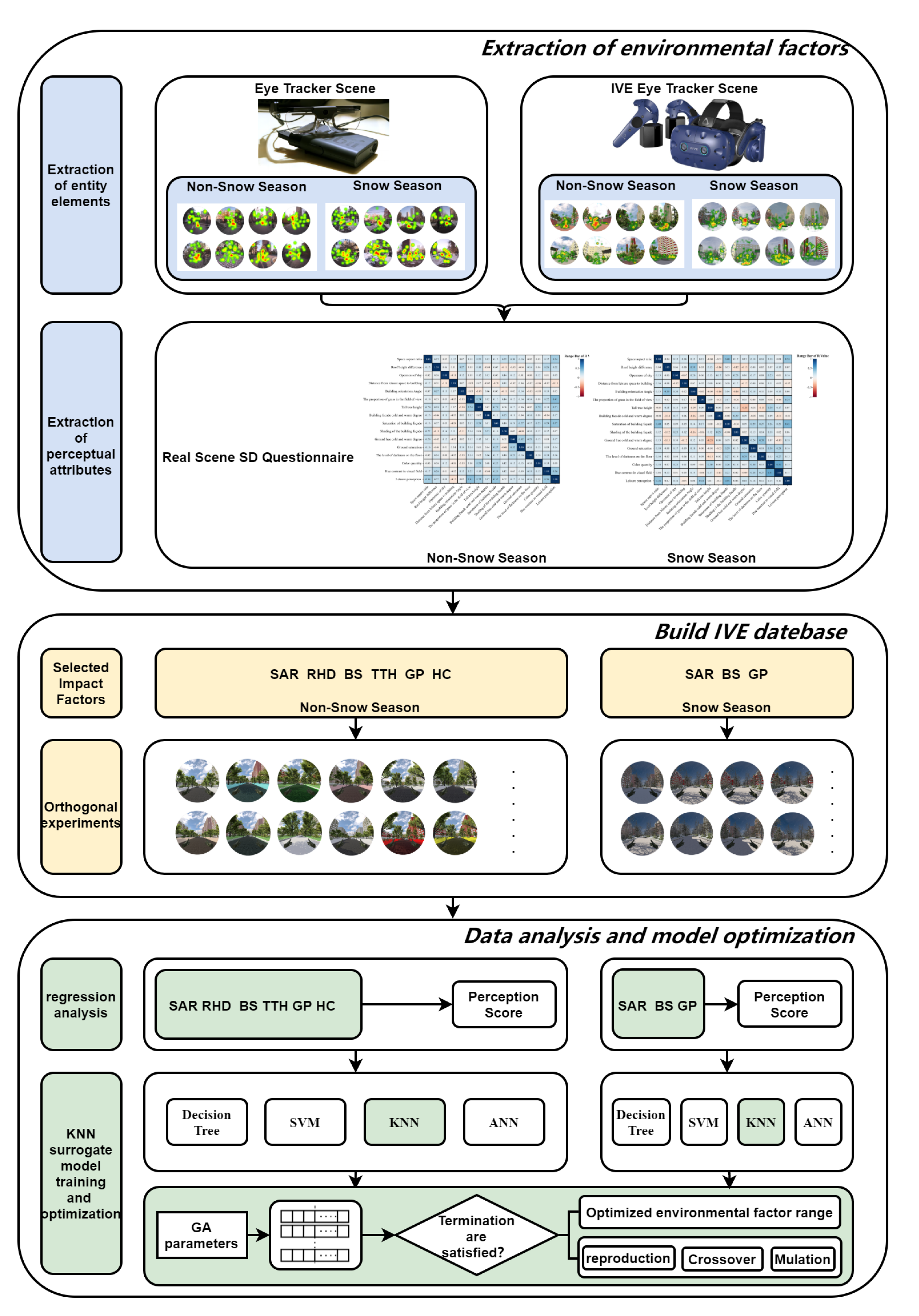
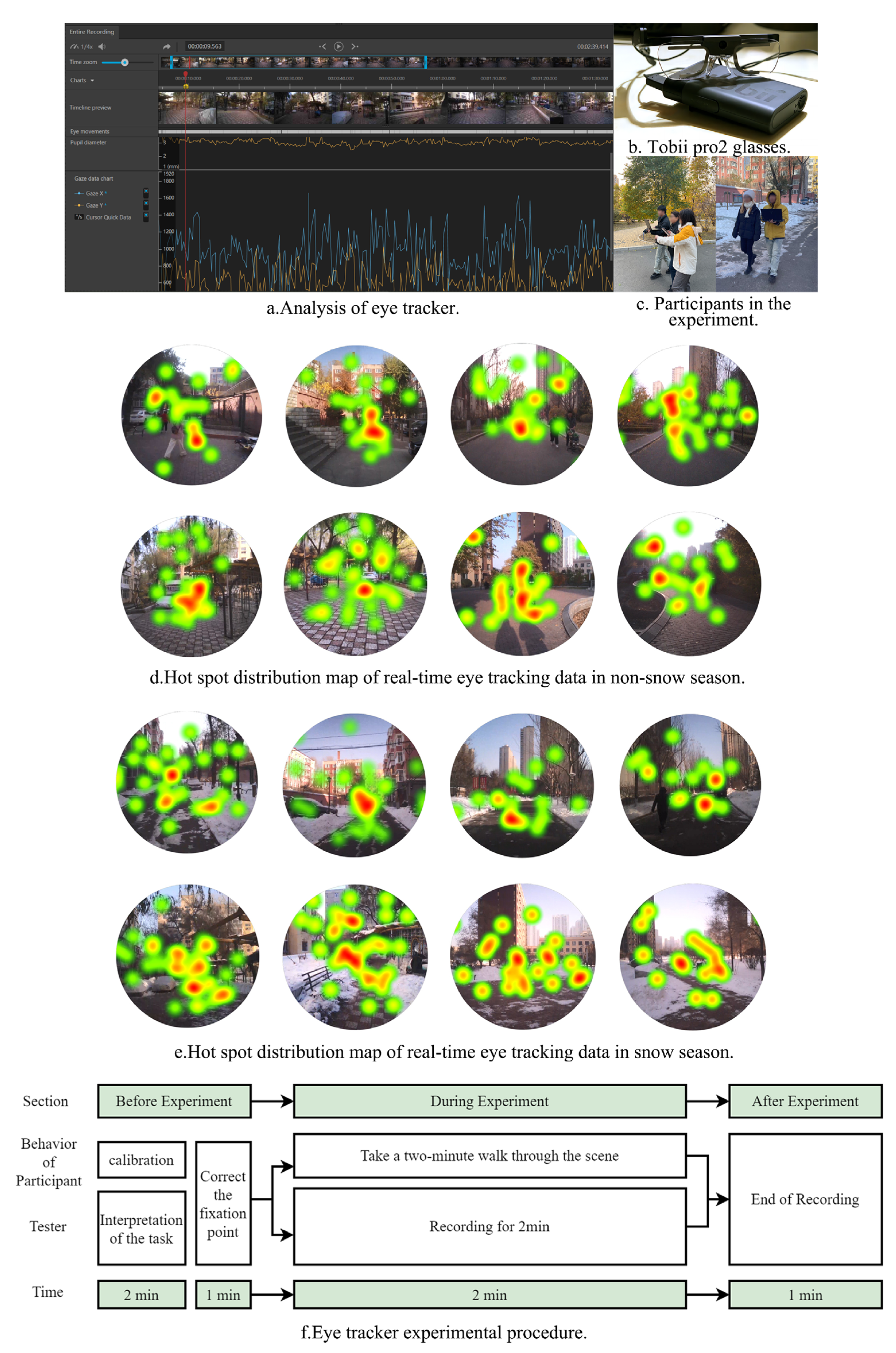
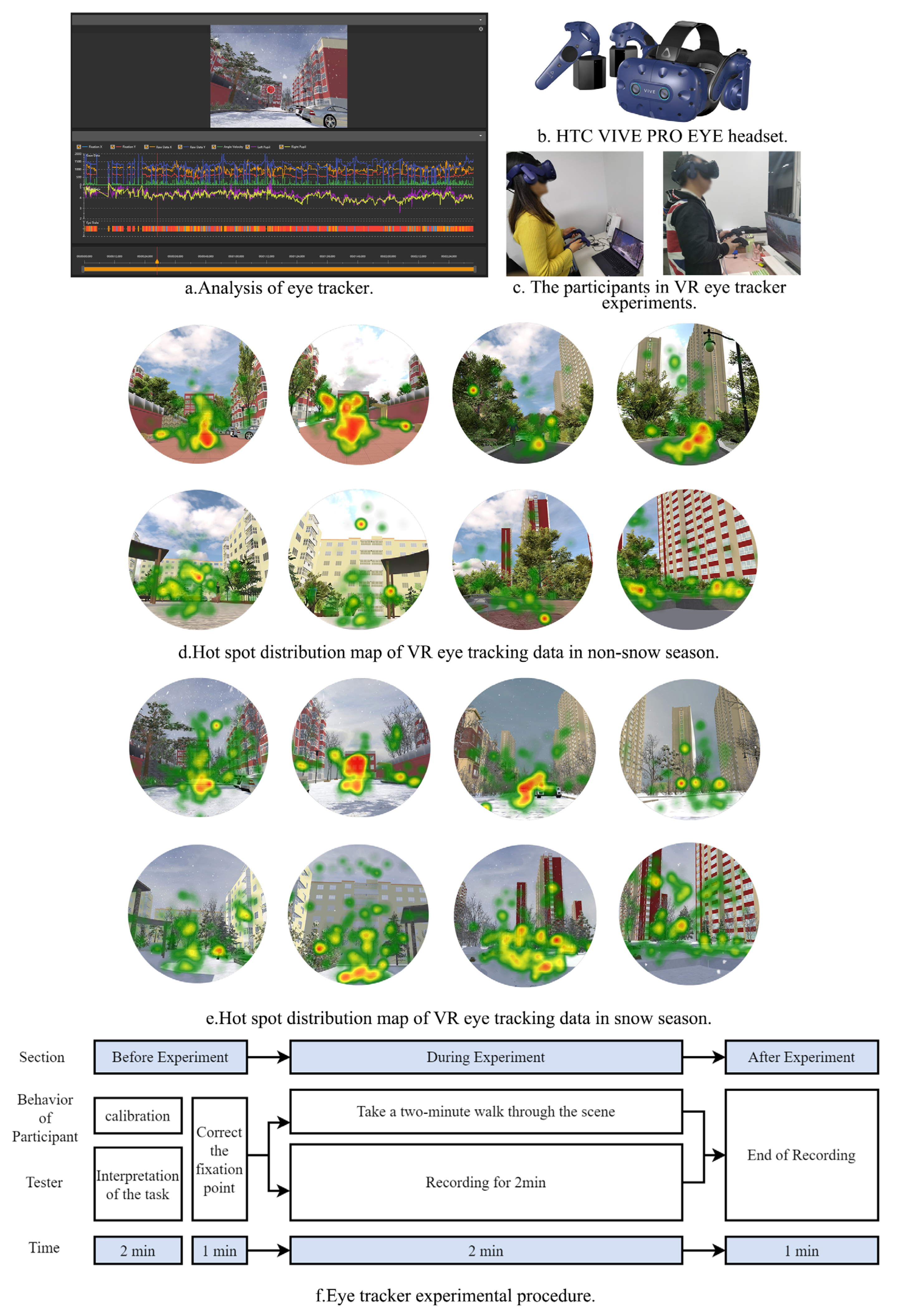
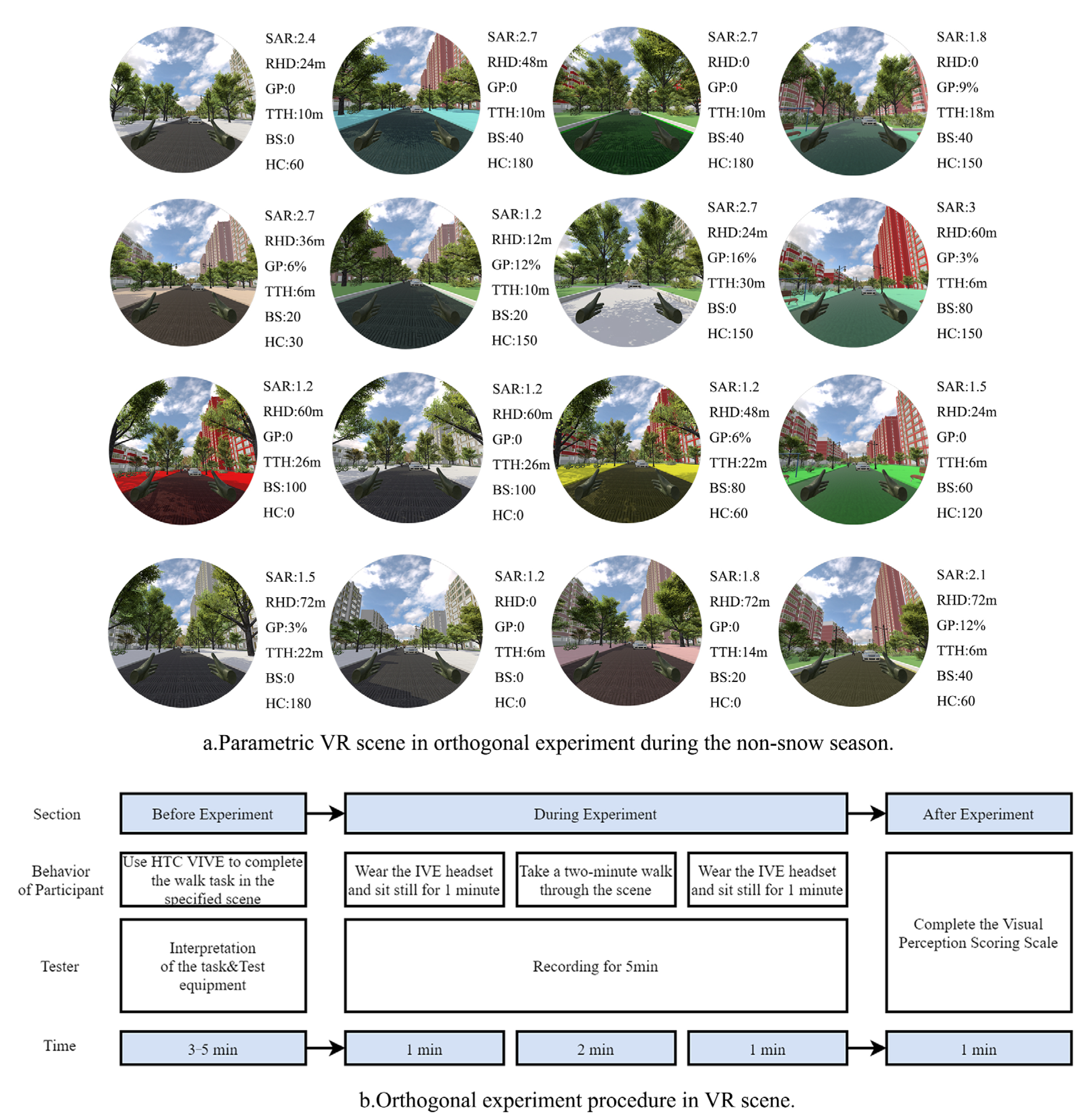
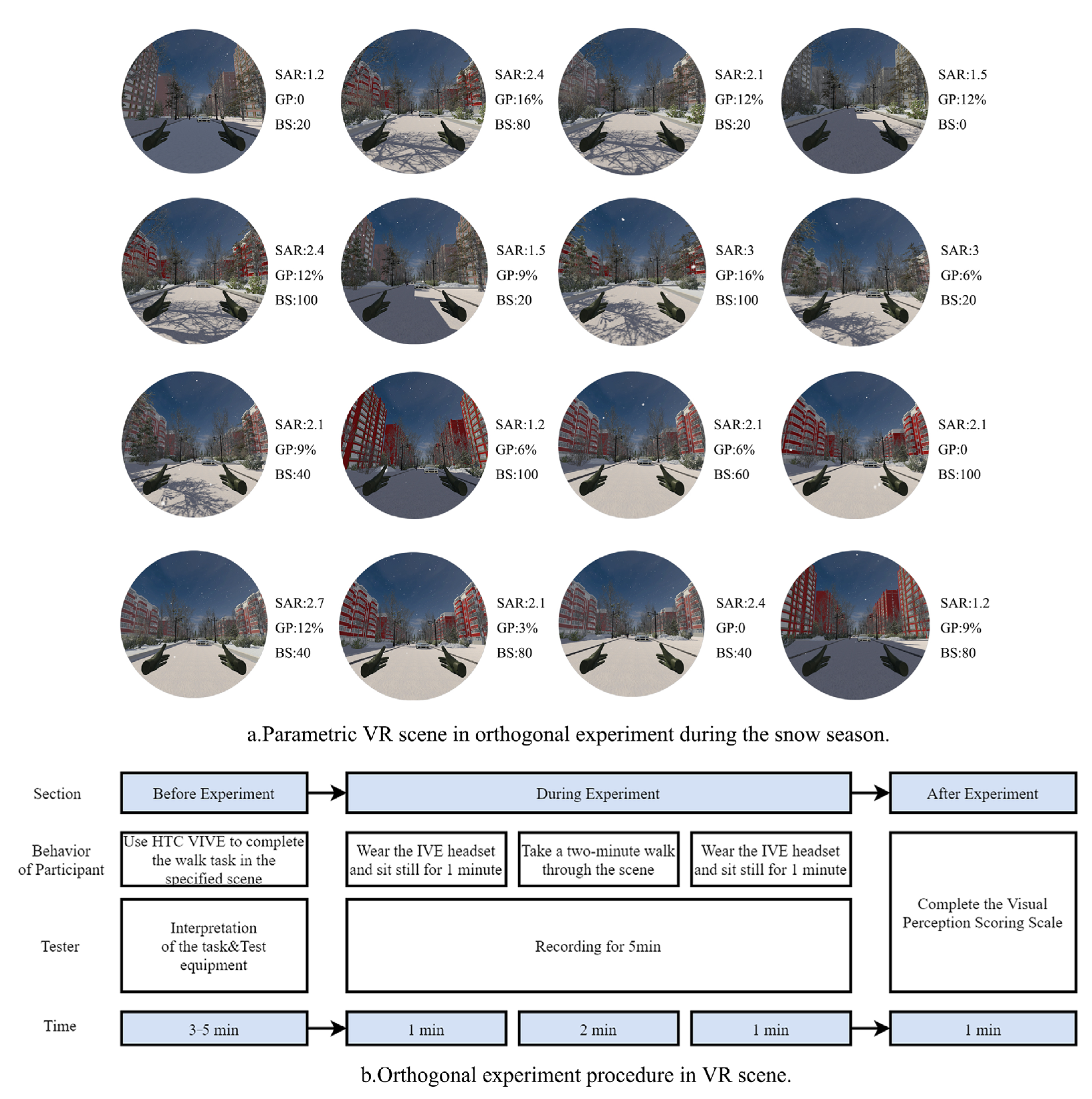
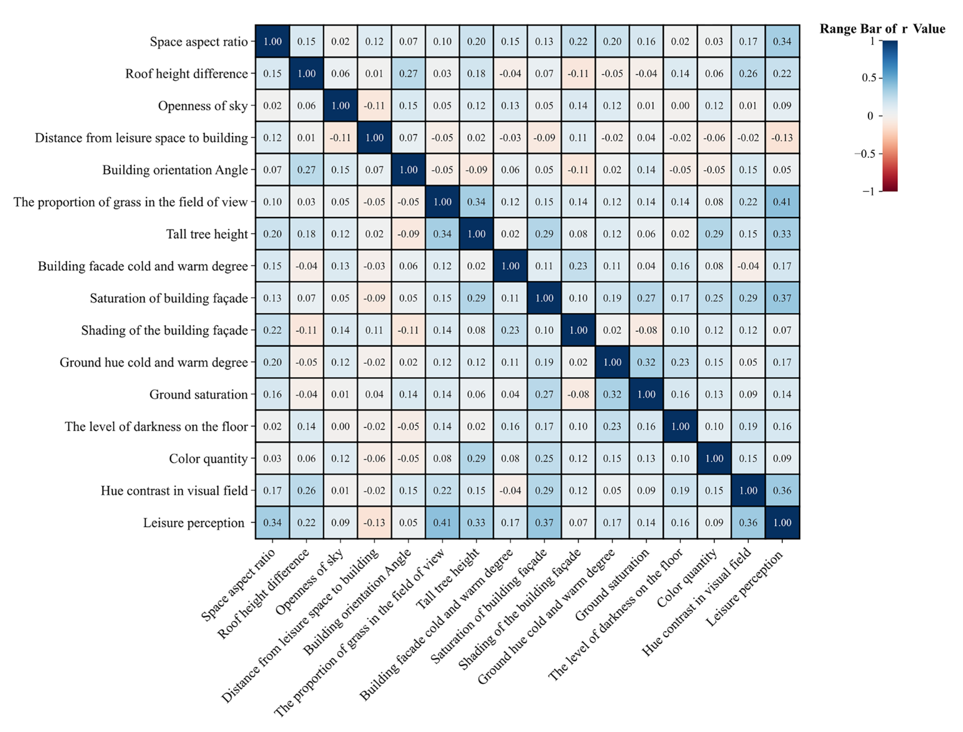
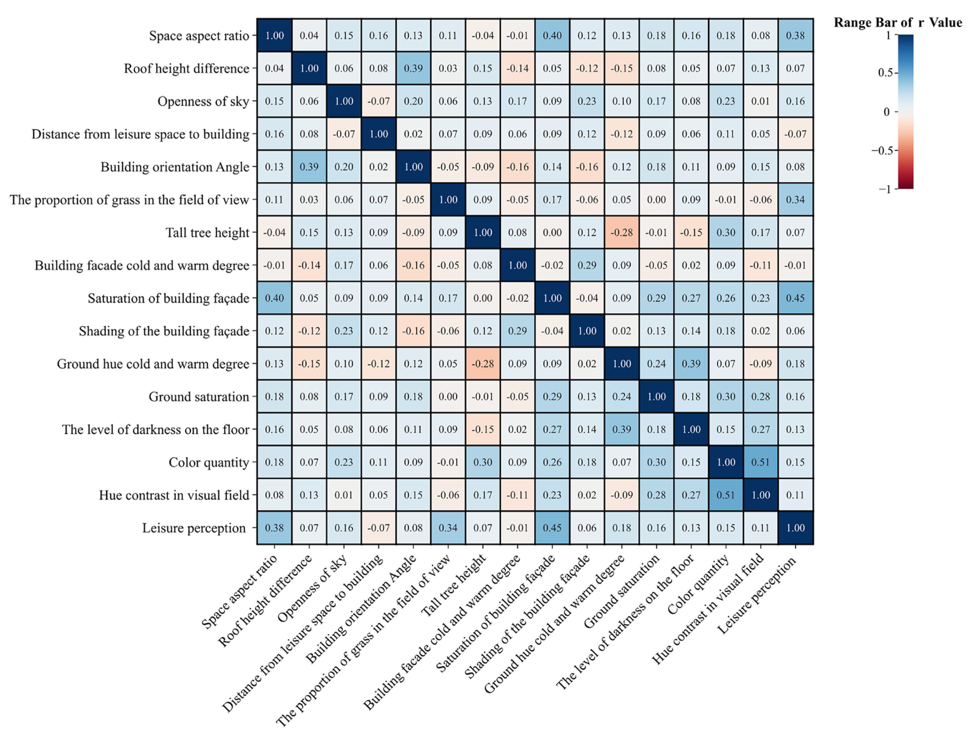
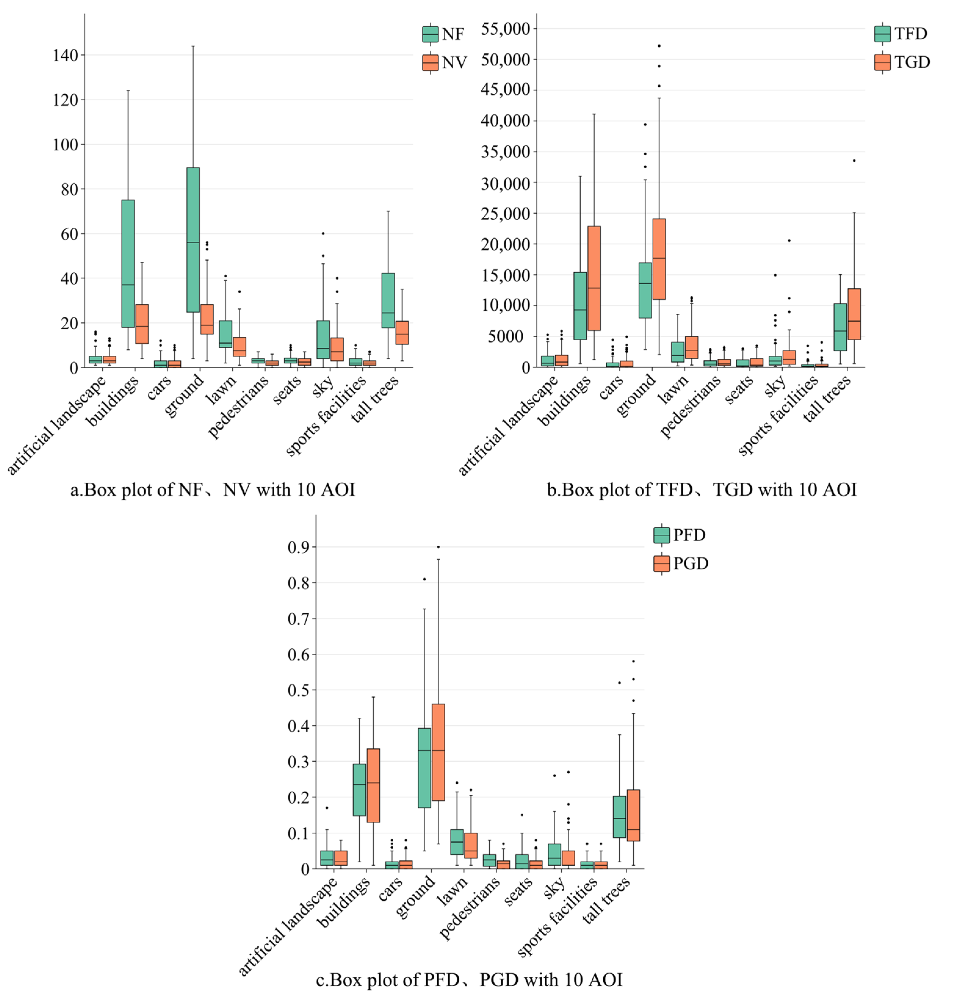
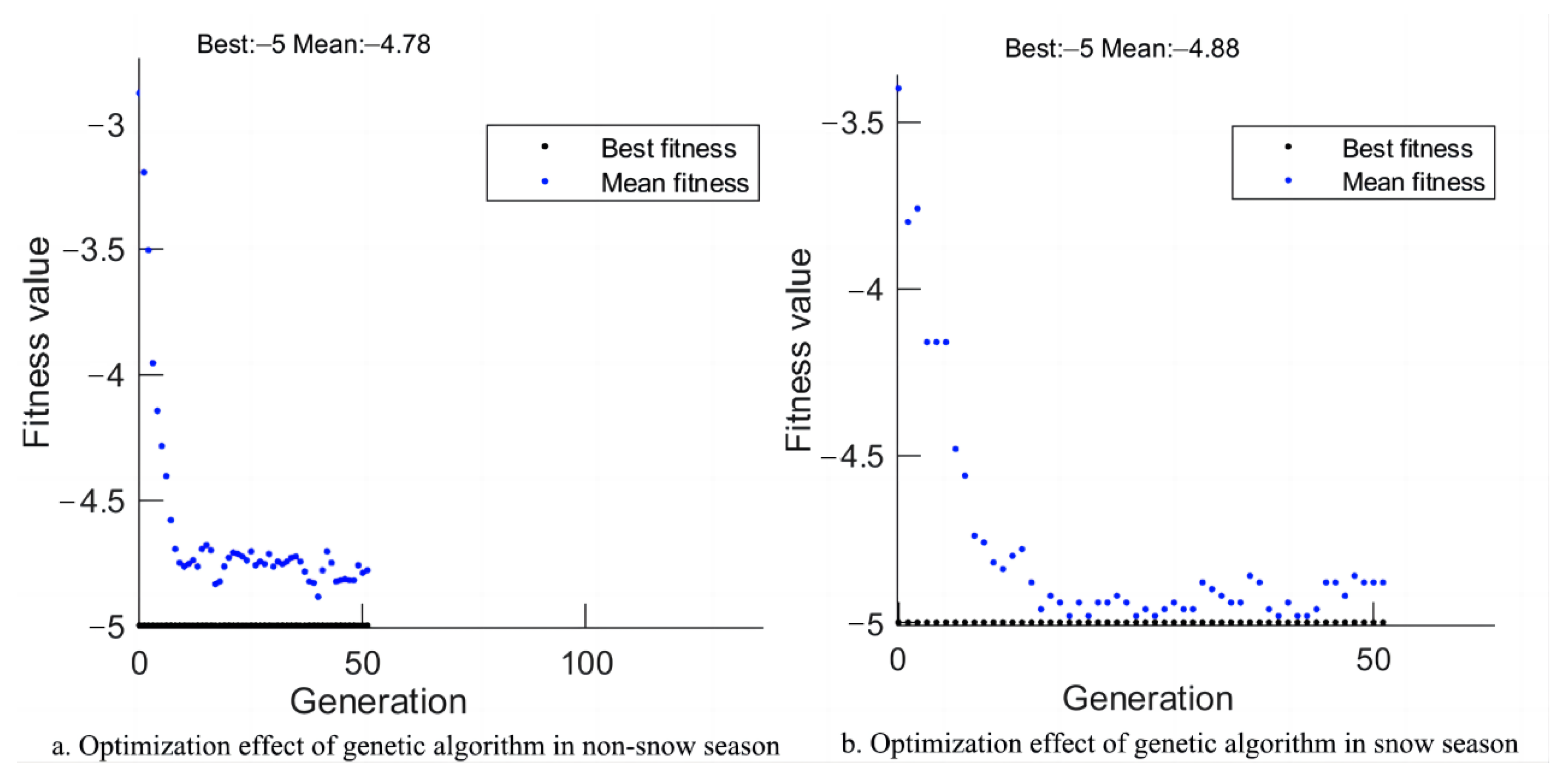
Table 1.
Inter-house landscape spaces in survey (the pictures in the table below were taken in real life and are only used to illustrate the research location, so they were not matched in terms of composition).
Table 1.
Inter-house landscape spaces in survey (the pictures in the table below were taken in real life and are only used to illustrate the research location, so they were not matched in terms of composition).
| Case | A | B | C | D |
|---|---|---|---|---|
| Construction time | 1990 | 2000 | 2013 | 2016 |
| Floor area ratio | 2.5 | 2.1 | 2.1 | 2.5 |
| Green space ratio | 24% | 20% | 30% | 30% |
| Live photos (non-snow season) |  |  |  |  |
| Live photos (snow season) |  |  |  |  |
Table 2.
Adjective pairs in SD questionnaire.
| Number | Factors | Adjective Pairs |
|---|---|---|
| 1 | Space aspect ratio | Narrow–wide |
| 2 | Roof height difference | Low–high |
| 3 | Openness of sky | Small–big |
| 4 | Distance from leisure landscape space to building | Near–far |
| 5 | Building orientation angle | Low–high |
| 6 | The proportion of grass in the field of view | Low–high |
| 7 | The height of tall trees | Low–high |
| 8 | Color of buildings—H | Cold–warm |
| 9 | Color of buildings—S | Low–high |
| 10 | Color of buildings—V | Darkness–brightness |
| 11 | Color of ground—H | Cold–warm |
| 12 | Color of ground—S | Low–high |
| 13 | Color of ground—V | Darkness–brightness |
| 14 | Color quantity | Little–much |
| 15 | Hue contrast in visual field | Small–large |
 | ||
Table 3.
Orthogonal experimental parameters in the non-snow season.
| Environmental Factors | Orthogonal Experimental Parameters in the Non-Snow Season |
| Space aspect ratio (SAR) | 1.2, 1.5, 1.8, 2.1, 2.4, 2.7, and 3 |
| Roof height difference (RHD) | 0 m, 12 m, 24 m, 36 m, 48 m, 60 m, and 72 m |
| Color saturation of buildings (BS) | 0, 20, 40, 60, 80, and 100 |
| Tall-tree height (TTH) | 6 m, 10 m, 14 m, 18 m, 22 m, 26 m, and 30 m |
| The proportion of grass in the field of view (GP) | 0, 3%, 6%, 9%, 12%, and 16% |
| Hue contrast in the visual field (HC) | 0, 30°, 60°, 90°, 120°, 150°, and 180° |
Table 4.
Orthogonal experimental parameters in the snow season.
| Environmental Factors | Orthogonal Experimental Parameters in the Snow Season |
|---|---|
| Space aspect ratio (SAR) | 1.2, 1.5, 1.8, 2.1, 2.4, 2.7, and 3 |
| Saturation of buildings (BS) | 0, 20, 40, 60, 80, and 100 |
| The proportion of grass in the field of view (GP) | 0, 3%, 6%, 9%, 12%, and 16% |
Table 5.
Optimized thresholds of non-snow environmental factors by GA.
| Solution Set 1 | Solution Set 2 | Solution Set 3 | Solution Set 4 | … | Solution Set 30 | Range | |
|---|---|---|---|---|---|---|---|
| SAR | 1.8795 | 1.9057 | 1.821 | 1.9776 | … | 2.1485 | 1.82–2.15 |
| RHD (m) | 15.094 | 10.8099 | 15.9183 | 18.1143 | … | 20.093 | 10.81–20.09 |
| BS | 58.2669 | 60.2785 | 48.5304 | 52.8396 | … | 61.0109 | 48.53–61.01 |
| TTH (m) | 17.5717 | 16.7644 | 14.3164 | 17.3361 | … | 18.2912 | 14.18–18.29 |
| GP (%) | 0.125 | 0.1369 | 0.1185 | 0.146 | … | 0.154 | 0.12–0.15 |
| HC | 19.9477 | 18.6411 | 20.6017 | 25.8764 | … | 26.8322 | 18.64–26.83 |
| W (Predict) | 5 (4.90) | 5 (4.70) | 5 (4.85) | 5 (4.96) | … | 5 (4.84) | 5 (4.70–5.0) |
Table 6.
Optimized thresholds of snow environmental factors by GA.
| Solution Set 1 | Solution Set 2 | Solution Set 3 | Solution Set 4 | … | Solution Set 30 | Range | |
|---|---|---|---|---|---|---|---|
| SAR | 2.2234 | 2.4057 | 2.5211 | 2.3716 | … | 2.5425 | 2.22–2.54 |
| BS | 68.5324 | 70.8215 | 78.5304 | 72.8396 | … | 82.3412 | 68.53–82.34 |
| GP (%) | 0.104 | 0.139 | 0.115 | 0.136 | … | 0.144 | 0.1–0.14 |
| W (Predict) | 5 (4.76) | 5 (4.80) | 5 (4.90) | 5 (4.67) | … | 5 (4.84) | 5 (4.67–4.90) |
Disclaimer/Publisher’s Note: The statements, opinions and data contained in all publications are solely those of the individual author(s) and contributor(s) and not of MDPI and/or the editor(s). MDPI and/or the editor(s) disclaim responsibility for any injury to people or property resulting from any ideas, methods, instructions or products referred to in the content. |
© 2024 by the authors. Licensee MDPI, Basel, Switzerland. This article is an open access article distributed under the terms and conditions of the Creative Commons Attribution (CC BY) license (https://creativecommons.org/licenses/by/4.0/).
Share and Cite
MDPI and ACS Style
Li, X.; Huang, K.; Zhang, R.; Chen, Y.; Dong, Y. Visual Perception Optimization of Residential Landscape Spaces in Cold Regions Using Virtual Reality and Machine Learning. Land 2024, 13, 367. https://doi.org/10.3390/land13030367
AMA Style
Li X, Huang K, Zhang R, Chen Y, Dong Y. Visual Perception Optimization of Residential Landscape Spaces in Cold Regions Using Virtual Reality and Machine Learning. Land. 2024; 13(3):367. https://doi.org/10.3390/land13030367
Chicago/Turabian StyleLi, Xueshun, Kuntong Huang, Ruinan Zhang, Yang Chen, and Yu Dong. 2024. "Visual Perception Optimization of Residential Landscape Spaces in Cold Regions Using Virtual Reality and Machine Learning" Land 13, no. 3: 367. https://doi.org/10.3390/land13030367
Note that from the first issue of 2016, this journal uses article numbers instead of page numbers. See further details here.