

Identifying the Optimal Area Threshold of Mapping Units for Cultural Ecosystem Services in a River Basin


1
Department of Landscape Architecture, College of Architecture and Urban Planning, Tongji University, Shanghai 200092, China
2
Joint Laboratory of Ecological Urban Design (Research Centre for Land Ecological Planning, Design and Environmental Effects, International Joint Research Centre of Urban-Rural Ecological Planning and Design), College of Architecture and Urban Planning, Tongji University, Shanghai 200092, China
*
Author to whom correspondence should be addressed.
Land 2024, 13(3), 346; https://doi.org/10.3390/land13030346
Submission received: 24 January 2024
/
Revised: 4 March 2024
/
Accepted: 6 March 2024
/
Published: 8 March 2024
(This article belongs to the Special Issue Urban Ecosystem Services IV)
Abstract
:Mapping cultural ecosystem services (CES) in river basins is crucial for spatially identifying areas that merit conservation due to their significant CES contributions. However, precise quantification of the appropriate area of mapping units, which is the basis for CES assessment, is rare in existing studies. In this study, the optimal area threshold of mapping units (OATMU) identification, consisting of a multi-dimensional indicator framework and a methodology for validation, was established to clarify the boundary and the appropriate area of the mapping units for CES. The multi-dimensional indicator framework included geo-hydrological indicator (GI), economic indicator (EI) and social management indicator (SMI). The OATMU for each indicator was determined by seeking the inflection point in the second-order derivative of the power function. The minimum value of the OATMU for each indicator was obtained as the OATMU for CES. Finally, the OATMU for CES was validated by comparing it with the area of administrative villages in the river basin. The results showed the OATMU for CES was 3.60 km2. This study adopted OATMU identification, with easy access to basic data and simplified calculation methods, to provide clear and generic technical support for optimizing CES mapping.
1. Introduction
The benefits provided by ecosystems and appropriated by humans are called Ecosystem Services (ES) [1]. According to the Millennium Ecosystem Assessment, ESs are classified into four categories: provisioning, regulating, supporting, and cultural services, each contributing uniquely to various aspects of human well-being [2]. Cultural ecosystem services (CES) are the non-material benefits obtained from ecosystems and are classified into 10 main subcategories: recreation and tourism, aesthetics, spiritual values, education, inspirational values, cultural diversity, knowledge systems, sense of place and identity, social relations, and cultural heritage values [2]. CES are fundamentally shaped and sustained by ecological, economic, and social factors [2,3,4]. However, the rapid pace of urbanization poses significant challenges, leading to ecosystem fragmentation and functional degradation, which in turn diminishes the CES supply capacity [5]. As a key to society, CES must be more thoroughly acknowledged as crucial for enhancing human health and demand increased attention from policymakers [6].
Through a long history of human interaction with nature, river basins have become densely populated human settlements and indispensable birthplaces of civilization [7]. The role of river basins in providing CES—such as cultural heritage, recreation and ecotourism, and aesthetic appreciation—is widely recognized [8]. These areas are considered the foundational units for ecosystem conservation planning and are deemed appropriate scales for the management of CES [9]. CES mapping in river basins is primarily used to concretely visualize the value of an area, allowing for an intuitive analysis of whether the supply and demand of CES are balanced [9]. Areas with a high CES supply, often characterized by abundant recreational activities or cultural values, contribute significantly to human health and are therefore critical to identify and prioritize for enhanced conservation efforts [6]. Given the relatively high value of CES attributed to aquatic areas [10], it is of paramount importance to conduct CES mapping studies in river basins.
However, without a clear understanding of the mapping units, the protection and development of CES will be hampered [11]. To divide these units, Campos-Campos et al. [12] analyzed variations in landscape units through the Supervised Classification method, while Alvioli et al. [13] introduced an automated approach utilizing the r.slopeunits v1.0 software for delineation. Currently, the mapping units for CES in river basins mainly consist of existing grid cells [14], land-use units [15], homogeneous landscape units [16], and administrative units [17]. In addition, different scales of catchments are applied to measure CES supply and demand in river basins [18,19]. Recognized as units that encapsulate ecological, social, economic, and cultural dimensions [11], catchments are extensively applied as mapping units in the fields of Hydrology and Geography [13,20,21]. There is a well-established and systematic method for delineating catchment boundaries using the ArcGIS 10.8 software hydrological analysis tool [21,22]. With clear boundaries that match the natural geographic extent of river basins, catchments avoid the problem of incompatibility between the boundaries of the mapping units and the study area.
The selection of mapping units profoundly affects the conclusions drawn from the CES assessment because the area of these units determines the credibility of the spatial images [11]. However, the determination of the appropriate area of mapping units has been largely neglected [23], leading to inadequate representation of the study area’s characteristics and compromised mapping accuracy [24]. Particularly when the precision of mapping units falls below that of the socio-practical system, there is a notable deficiency in motivation or comprehensive guidelines for their application [11]. Therefore, with the establishment of appropriate units, CES can be accurately quantified [25]. Several studies in environmental hydraulics have used multiple catchment area thresholds for selecting the optimal area thresholds to obtain relatively homogeneous and refined mapping units [20,22,26]. To enhance mapping precision alongside computational efficiency, this study introduced the concept of area threshold, offering both a theoretical framework and a practical approach for accurately determining the appropriate area of mapping units. The area threshold of mapping units (ATMU) is defined as the minimum area of mapping units. The optimal area threshold of mapping units (OATMU) is defined as the ATMU that most effectively fulfills the objectives of the study, thereby enhancing the precision of the outcomes and accurately reflecting the characteristics of the study area [22]. The value of OATMU, which determines the most appropriate area of mapping units, varies according to the research objectives and is highly related to the indicator selection. For instance, in the pursuit of accurately delineating actual river networks and catchment boundaries, drainage density serves as a key indicator for determining the OATMU [22].
This study mainly focused on (1) clarifying the boundary and the most appropriate area of the mapping units for CES; (2) determining the indicators affecting the area of the mapping units and methods of their calculation; and (3) testing the applicability of OATMU identification methods for CES in river basins. As a cornerstone in the research on CES spatial mapping, this study has constructed a novel, streamlined, and transferable method that leverages available spatial data to identify the optimal area for mapping units with high precision. By tackling the earlier challenges of subjective selection of mapping unit types and the absence of quantitative assessments of their areas, this study significantly advanced the precise application of CES quantification and supply demand research outcomes in real-world spaces.
2. Materials and Methods
2.1. Study Area
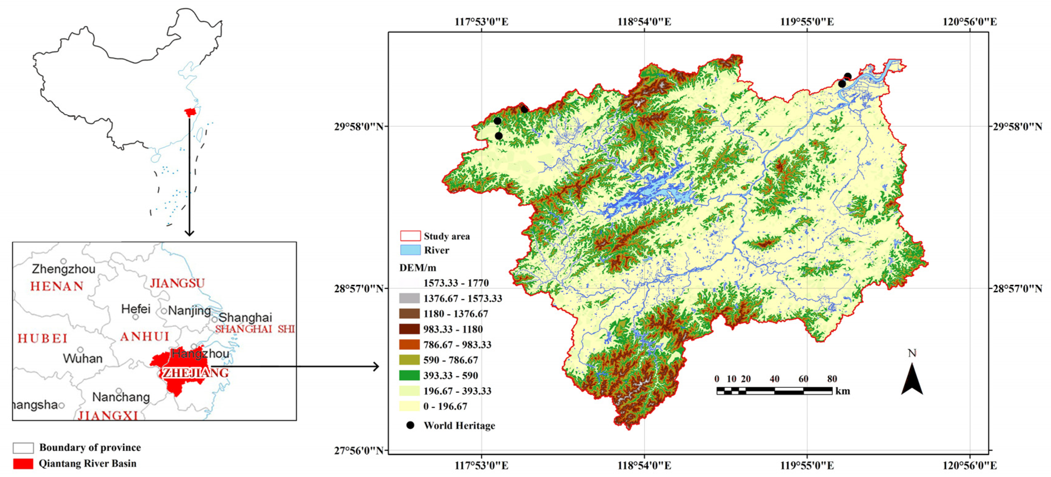
The Qiantang River Basin is located in southeastern China, covering an area of 42,770.05 km2 (116°52′ to 120°56′ E, 27°56′ to 30°59′ N) (Figure 1). The whole river, with a length of 668.10 km, is the longest river in Zhejiang Province. As of the end of 2020, the basin boasted a population of 12,667,200 and a GDP of approximately 1.65 trillion dollars [27]. As one of the top ten practices of Nature-Based Solutions jointly published by the Chinese Ministry of Natural Resources and the World Conservation Union (IUCN), the Qiantang River Basin serves as a pilot location for developing and demonstrating a replicable and scalable model of key ecological functional zones across the nation [27].
There are 3 reasons for choosing the Qiantang River Basin as the study area: (1) Diverse Geomorphology for CES Spatial Analysis. The Qiantang River Basin is a representative region featuring a wide range of catchment geomorphic types, including mountains, basins, and plains [28]. This diversity in topographic features across different catchments yields a variety of CES [8]. (2) Rich and Emblematic Cultural Heritage. Serving as a cradle of ancient Chinese civilization, the basin is closely linked with four World Heritage sites: Huangshan Mountain, West Lake, the Grand Canal, and ancient villages in southern Anhui province, such as Xidi and Hongcun. It is also home to the renowned Liangzhu Culture (5300–4200 cal. a BP) and Hui Culture (1121–1911), making it a region of significant cultural value [28]. (3) Challenges Posed by Rapid Urbanization. As one of the most densely populated and economically advanced areas in China, the Qiantang River Basin faces threats from fast-paced urbanization, which leads to the encroachment and fragmentation of CES areas. Notably, the construction of hydroelectric power plants has contributed to the loss of numerous historical sites. This underscores the critical need for a systematic and accurate approach to CES space optimization within the basin.
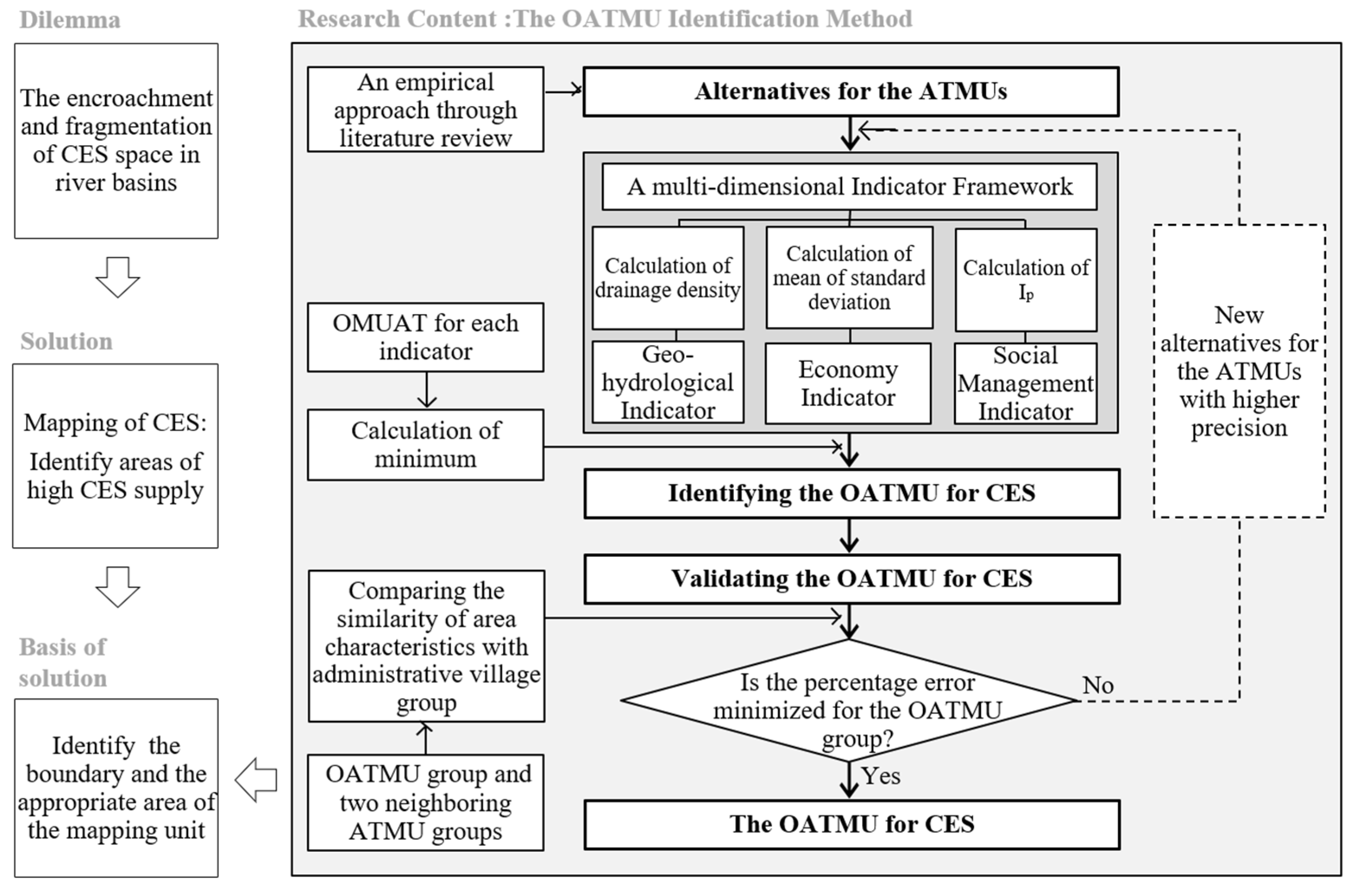
2.2. Research Framework
As a foundational study of CES mapping, the OATMU identification method was constructed to identify the boundary and the most appropriate area of the mapping units. Distinct from other ESs, the assessment of CES leans heavily on human perceptions, cultural values, and demands [29]. Consequently, incorporating indicators that reflect economic and social dimensions is crucial. Based on ecological, economic and social aspects, a multi-dimensional indicator framework with specific indicator calculation methods and the validation of the final results were established in this study (Figure 2).
2.3. Data Sources and Preprocessing
Five data sets were used to calculate the OATMU: the digital elevation model (DEM), China population spatial distribution data, China GDP spatial distribution data, China administrative boundary data and the point of interest (POI) (Table 1).
Among these, the China population spatial distribution data and China GDP spatial distribution data have not been updated in recent years; thus, the most recent data from 2019 were used. At Amap Company, one of China’s most popular mapping services, POI data were categorized into 23 types using classification codes. For this study, POI data for government organizations and social groups within the study area were collected, amounting to 57,644 records.
The projection coordinate system for the aforementioned data was converted to WGS 1984 UTM Zone 50N. Spatial data processing was conducted using ArcGIS 10.8.
2.4. Alternatives for ATMUs
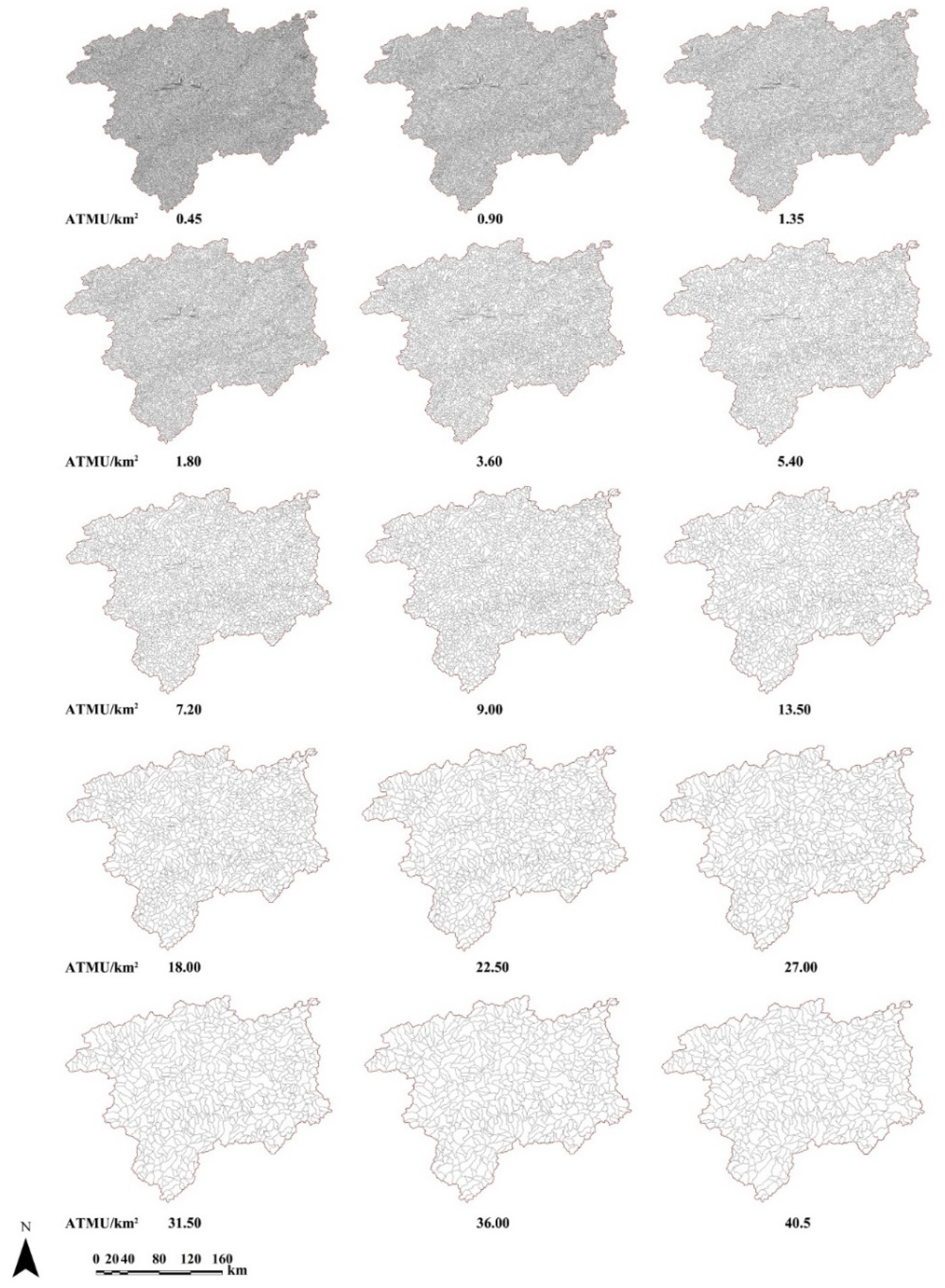
The ATMUs are typically determined by the number of grids with different DEM accuracies [22] or by the limitations of available computing memory [30]. This study established the ATMUs based on the following criteria: (1) Integration of ecological and social research findings. For social ecosystems, the average area of mapping units is 3.50 km2 [23]. Consistent with studies of river basins of comparable size, the OATMUs range from 1.41 to 7.20 km2 at the ecological and social levels. (2) Accuracy Assurance. Available studies offer a range of 6 to 15 alternatives (Table 2). Finer ATMUs and a greater number of alternatives lead to more accurate results [22,31]. To ensure precision, this study adopts the maximum number of alternatives for calculations. (3) Maximizing the OATMU range of values. The upper limit was increased to the maximum reported value of 40.5 km2 in existing studies (Table 2). (4) Grid Multiplicity [22]. The ATMU is an integer multiple of the number of grids. In this study, with a DEM data accuracy of 30 m and each grid area being 30 m × 30 m, the ATMU is an integer multiple of 0.0009 km2.
In summary, following the research of Zhang [32], this study selected 15 alternatives with 500, 1000, 1500, 2000, 4000, 6000, 8000, 10,000, 15,000, 20,000, 25,000, 30,000, 35,000, 40,000, and 45,000 grids. The calculation formula for each alternative is as follows:
where is the ATMU of jth alternative, is the area of grid, is the number of grids of jth alternatives.
Consequently, the 15 alternatives of ATMUs were determined to be 0.45 km2, 0.90 km2, 1.35 km2, 1.80 km2, 3.60 km2, 5.40 km2, 7.20 km2, 9.00 km2, 13.50 km2, 18.00 km2, 22.50 km2, 27.00 km2, 31.50 km2, 36.00 km2, 40.50 km2.
Utilizing the four-step process of terrain preprocessing, flow direction identification, ATMU setting, and catchment extraction in the Hydrological Analysis module of ArcGIS 10.8 software [22], 15 catchment alternatives were generated. Patches smaller than the ATMU were automatically eliminated to optimize the ATMU alternatives.
2.5. Indicator Framework
The following criteria were utilized to select the OATMU for CES: (1) Covering ecological, economic and social aspects [3,4]; (2) Data availability, accessibility and reliability; (3) Representativeness of indicators for core characteristics. In summary, 3 indicators were selected to identify the OATMU for CES: the geo-hydrological indicator (GI), economy indicator (EI), and the social management indicator (SMI).
2.5.1. Geo-Hydrological Indicator
The drainage density was used as a proxy for the geomorphologic and hydrologic characteristics of river basins [35]. The drainage density, which shows a strong correlation with surface roughness, vegetation index, and water storage changes, is better modeled and more generalizable [36]. Hence, the drainage density was selected to characterize GI. Its calculation formula is as follows:
where is the drainage density, i is the ith mapping unit, n is the maximum number of mapping units, Li is the river length in the ith mapping unit, and Ai is the area of the ith mapping unit.
2.5.2. Economy Indicator
GDP per capita is frequently utilized as a significant measurement of economic standards [37]. The level of economic development is similar in each mapping unit; therefore, the economic homogeneity within the mapping unit can be reflected by the degree of dispersion of GDP per capita.
The standard deviation is often utilized to depict the extent of data dispersion or aggregation uniformity in space [38]. Hence, the mean value of the standard deviation of GDP per capita was selected to represent EI. The formula is as follows:
where MSD is the mean standard deviation of GDP per capita, i is the ith mapping unit, n is the maximum number of mapping units, Si is the standard deviation of GDP per capita in the ith mapping unit.
2.5.3. Social Management Indicator
As one of the 3 dimensions of CES, social aspect includes a societal or shared interpretation at stake, as in social process, social scale, social problem, etc. [4]. Social management is crucial in the social aspect, as it often determines the specific preferences for management programs and the implementation of management decisions. Government organizations and social groups are the mainstays of social management. The greater the concentration of government organizations and social groups, the more likely it is to be a complete spatial unit with control, management, supervision and service functions [39]. Traditional methods such as the kernel density method use POI as a single data source [40], which failed to combine the mapping unit variables to reflect the differences among alternatives. The Index of Patchiness () is used in population ecology to measure the intensity of population aggregation by calculating patches occupied by the number of individuals [41]. Due to the need to clarify the spatial extent of study individuals and distribution patches, this study selected of POI for government organizations and social groups to illustrate SMI. The formula is as follows:
where is the index of mean crowding, P is the average number of POI for government organizations and social groups within each mapping unit. Where P is as follows:
where i is the ith mapping unit, n is the maximum number of mapping units, Pi is the number of POI for government organizations and social groups in the ith mapping unit. is as follows:
where S2 is the variance of the number of POI for government organizations and social groups in the mapping units from i to n.
2.6. Identification of the OATMU
The OATMU is typically determined by the inflection points on the relationship curve that illustrates the correlation between the indicator and ATMUs [42]. This method is not limited to calculating optimal area thresholds corresponding to drainage density but is also widely used to calculate optimal area thresholds for slope [43], socio-economic [44], and so on. Second-order derivative analysis is commonly used as a research method for extracting inflection points from relationship curves [45], with the advantages of computational simplicity and ascertainable results. The inflection point in this method is where the second derivative approaches 0 and no longer changes afterwards [46]. In this study, the second-order derivative of the fitting function curve was chosen to detect particular inflection points.
Through the Matlab R2020a software, the relationship between the 3 indicators and ATMUs was curve-fitted using the power function [47], the second-order derivatives of the power function were obtained, and the inflection point was identified [46]. The ATMU corresponding to the inflection point is the OATMU for each indicator.
When there are different OATMUs for each indicator, it is generally believed that the smallest OATMU is more conducive to fine-scale surface research [30,31]. To prevent the loss of spatial information during calculation, this study selected the minimum OATMU value from the 3 indicators as the OATMU for CES in river basins. The formula is as follows:
where , , is the OATMU corresponding to the inflection points of the GI, EI, and SMI, O is the OATMU for CES in the basin.
2.7. Validation of the OATMU for CES
As the practical units of a basin ecosystem, catchments do not coincide with the boundaries of administrative units [18], but often have strong correlations with them [48]. Administrative villages are the smallest administrative units and also have relatively complete social-ecological systems, often appearing as the basic units of cultural landscapes [49]. In this study, the validation of the OATMU for CES was carried out by measuring the similarity of area data between the mapping units and administrative villages. The mapping unit dataset with the OATMU for CES was defined as the OATMU group; the mapping unit dataset with the left ATMUs adjacent to the OATMU was defined left-OATMU group; the mapping unit dataset with the right ATMU adjacent to the OATMU was defined as the right-OATMU group; and the administrative village dataset within the Qiantang River Basin was defined as the administrative village group. By comparing the mean area, area quartile distance, and area maximum interval of the 3 ATMU groups and the administrative village group [26], the group with the minimum percent error of all three is the OATMU group for CES, and the corresponding ATMU is the OATMU for CES in the river basin. Validation was conducted using descriptive statistics and box plots in IBM SPSS Statistics 26 software.
3. Results
3.1. Characteristics of the Indicators
Fifteen alternatives for ATMUs were obtained through extraction and optimization. The mean area of mapping units for each alternative was concentrated between 1.05 and 92.62 km2 (Figure 3).
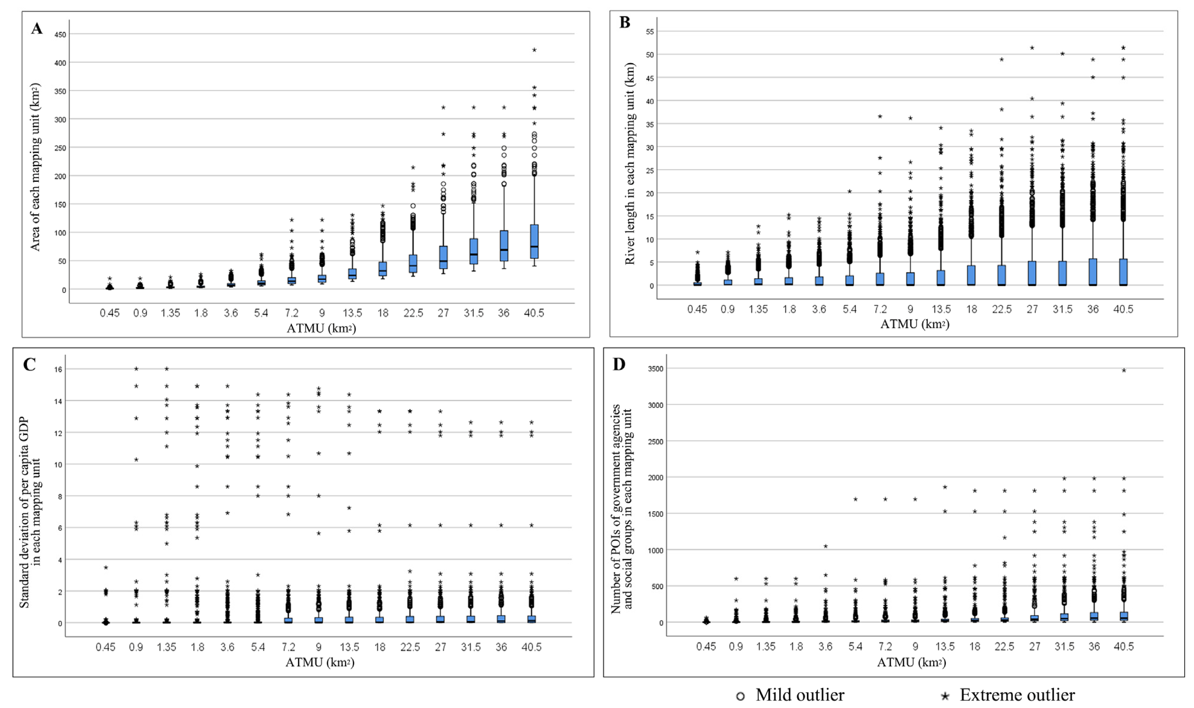
For GI, among the 15 alternatives, the minimum area of mapping units was 0.45 km2, and the maximum area was 421.52 km2 (Figure 4A). The average river length of 15 alternatives was concentrated at 0.45~3.93 km, with the shortest length of 0.03 km and the maximum length of 51.39 km (Figure 4B). For EI, GDP per capita varied considerably within each alternative, resulting in more extreme values. The minimum value of the standard deviation of GDP per capita within each mapping unit was 0, and the maximum value was 16.00 (Figure 4C). For SMI, the minimum number of POIs for government organizations and social groups in each mapping unit was 0, with the maximum reaching 3471 (Figure 4D).
3.2. Evaluation of the OATMU for CES
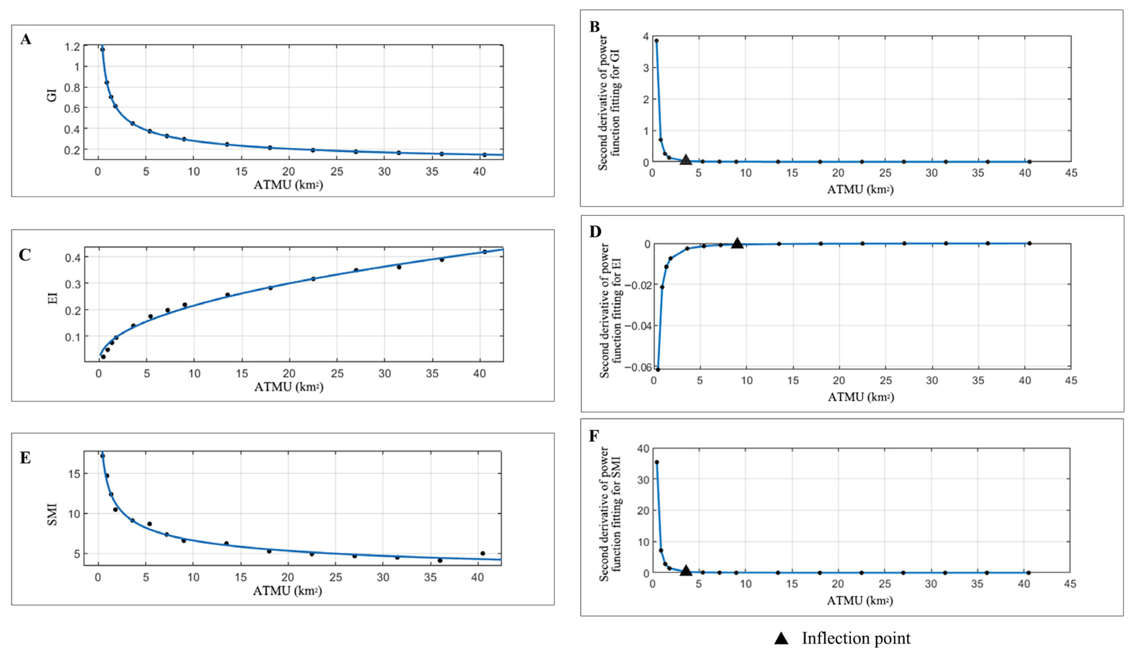
(1) The OATMU for GI
EI was used as the vertical axis, and ATMU was used as the horizontal axis. The power function used for curve fitting was , with a goodness-of-fit (Figure 5A). The second derivative of power function fitting for RE was (Figure 5B). The curve image plotted by Matlab showed the ATMU corresponding to the inflection point was 3.60 km2. For GI, the OATMU in the Qiantang River Basin was 3.60 km2.
(2) The OATMU for EI
EI was used as the vertical axis, and ATMU was used as the horizontal axis. The power function used for curve fitting was , with a goodness-of-fit (Figure 5C). The second derivative of power function fitting for SEI was (Figure 5D), and the ATMU corresponding to the inflection point was 9.00 km2. For EI, the OATMU in the Qiantang River Basin was 9.00 km2.
(3) The OATMU for SMI
SMI was used as the vertical axis, and ATMU was used as the horizontal axis. The power function used for curve fitting was , with a goodness-of-fit (Figure 5E). The second derivative of power function fitting for SMI was (Figure 5F), and the ATMU corresponding to the inflection point was 3.60 km2. For SMI, the OATMU in the Qiantang River Basin was 3.60 km2.
(4) The OATMU for CES
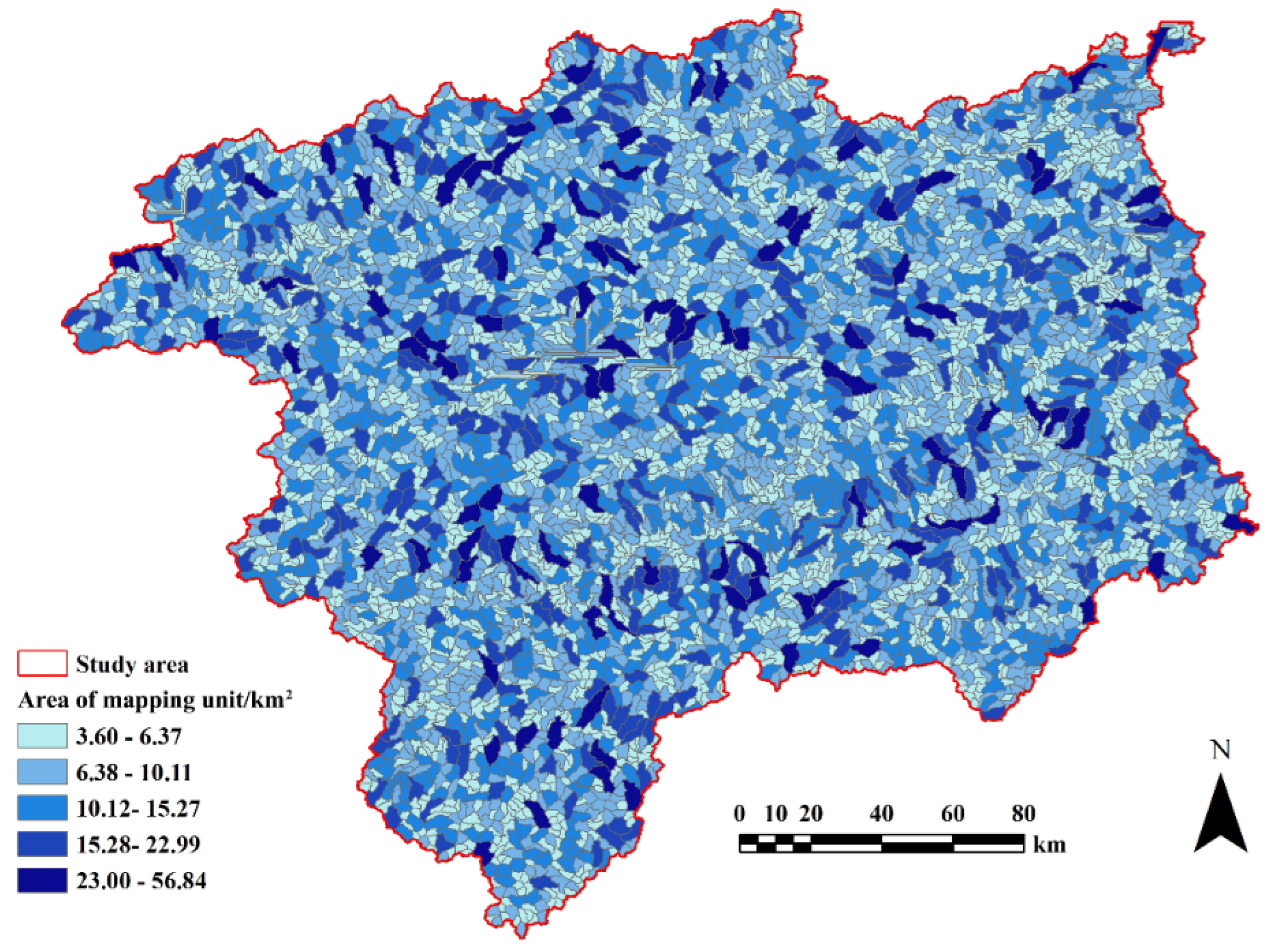
According to Equation (7), the OATMU for CES in the Qiantang River Basin was determined to be 3.60 km2. When the ATMU was 3.60 km2, the GI was 0.4592, the EI was 0.1383 and the SMI was 6.6596. There were 4910 mapping units in the OATMU dataset, of which the area of mapping units smaller than 6.37 km2 accounted for 46.74% of the total. The mapping units between 6.38 km2 and 10.11 km2 accounted for 29.04%. The mapping units between 10.12 km2 and 15.27 km2 accounted for 15.58% (Figure 6).
3.3. Validation of ATMUs Groups and Administrative Village Group
The OATMU group (3.60 km2), the left-OATMU group (1.80 km2), and the right-OATMU group (5.40 km2) were selected for validation with the administrative village group. The mean area of the administrative village group was 6.29 km2, with an interquartile range of 4.68 km2. The mean area of the left-OATMU group was 4.19 km2 with an error of 33.39% from the mean area of the administrative village group and an interquartile range of 2.64 km2 with an error of 43.59%. The mean area of the OATMU group was 8.23 km2 with an error of 30.84%, and the interquartile range was 5.16 km2 with an error of 10.26%. The mean area of the right OATMU group was 12.63 km2 with an error of 100.79% and the interquartile range was 8.19 km2 with an error of 75%. Compared to the left-OATMU and the right-OATMU groups, the boxplots for the administrative village group and the OATMU group were the most similar, with both sets of boxes clustered in the 0–10 km2, with the lower edges clustered in the 0–10 km2 and the upper edges clustered in the 10–20 km2 (Table 3).
The median area of the left-OATMU group was closer to that of the administrative village group. However, the range of the maximum value was 24.84 km2, which was significantly smaller than that of the administrative village group (63.42 km2). There is a risk that a large number of basic cultural landscape units could be divided excessively resulting in data redundancy. The minimum and mean values of the area for the right-OATMU group were much larger than the values of the administrative village group. For the right-OATMU group, the area of the mapping units was too large, resulting in decreased accuracy of the results. The percentage error of the mean area and quartile distance of the OATMU group was the smallest. In addition, the range and degree of data dispersion were most similar to those of the administrative village group, and it avoided the data redundancy caused by excessive delineation of basic cultural landscape units. Therefore, the OATMU for CES in the Qiantang River Basin was determined to be 3.60 km2.
4. Discussion
4.1. Applicability of the Multi-Dimensional Indicators and Calculation Methods
This study systematically identified the OATMU for CES by constructing a multi-dimensional indicator framework that includes GI, EI, and SMI. They were derived from Zhou et al., MEA, Scholte et al., Barnes and Hamylton, and Heasley et al. [2,3,36,41,50]. In contrast to previous studies that constructed a GI framework for river basin management [51], this study integrated EI and social SMI, adding two measurement dimensions (Figure 4) that yielded more systematic results.
For calculating GI, the drainage density method proves to be more effective for simulating areas with large topographic relief compared to the fitness index and fractal theory methods [52]. The difference in elevation in the Qiantang River basin is 1770 m (Figure 2). Combined with the actual situation of the study area, it is more reasonable to choose the drainage density method. Through the drainage density method, Zheng et al. [53] found that many parallel river networks were formed in areas with little change in elevation. This aligns with the results of the four alternatives for ATMUs, which take values between 0.45 km2 and 3.60 km2 (Figure 3). Additionally, as the ATMU becomes larger, the slope network chain is gradually eliminated, revealing the main rivers [53]. This is similar to the findings of this study (Figure 4B). The study areas have different locations and cover a wide range of scales (Table 2), which demonstrates the universality of the drainage density method for calculating GI.
For EI, the variability of GDP per capita between mapping units can be calculated by absolute differences, including standard deviations [50]. In this study, the mean value of the standard deviation of GDP per capita was used to reflect the differences for the EI of the mapping units, which facilitates cross-sectional comparisons of alternatives when there is only one value for each ATMU. In the absence of finer data sources, the standard deviation of GDP per capita within many mapping units is 0 for ATMUs smaller than or equal to 9 km2 (Figure 4C), which is consistent with the study of Liang et al. [54]. The large degree of data dispersion (Figure 4C) indicated that the economic distribution of the Qiantang River Basin is not uniform and that there are large differences in economic development between different mapping units, which is consistent with the study of Zhou et al. and Wang et al. [55,56].
For SMI, was introduced to explore the possibility that the clustering pattern of POIs varies with the spatial scale of the mapping unit. The distribution of POI for government organizations and social groups, whose primary function is management and accessibility, is geospatially relevant. The 15 ATMUs from 0.45–40.5 km2 all have a number of POIs within a single mapping unit of 0 (Figure 4D), due to the fact that those mapping units are located in large bodies of water or in mountainous areas that are not easily accessible (Figure 2). The presence of large ecological reserves with geomorphological diversity limits the spatial distribution of POIs, which is consistent with Zhen et al. [57]. The maximum value of the number of POIs within a single mapping unit reaches 3471, and the minimum value is 0 (Figure 4D). Such a huge difference in the extreme value of the number for POI reflects the imbalance of the social management situation in the Qiantang River Basin, which is in line with the study of Li [58].
4.2. Identification and Comparison of the OATMUs for Each Indicator
Based on the conclusion from the existing literature, this study applied the method that accurately identified the OATMU by fitting the second-order derivative of the power function [46]. Some studies exacted the OATMU by calculating the rate of reduction for the first-order derivative of the power function relationship [53] or the rate of change for the relation curve [26]. However, in the fitted curves for the three indicators of GI, EI, and SMI (Figure 5A,C,E), the rate of change for the relationship curves has been decreasing with the increase in ATMUs, and it becomes challenging to determine the corresponding OATMUs from the appropriate rate of change. Tang et al. used Matlab to calculate the OATMU by interpolating the data with a one-in-ten-thousand threshold [59]. However, since the area ratio of the study area to the mapping unit in this study is sufficiently large, refining the accuracy to 0.0009 km2 would result in a large amount of redundant computational data. Considering precision and ease of operation, this method, which was identified by fitting the second-order derivative of the power function, was used in this study for calculation.
In the Qiantang River Basin, the OATMU for GI was 3.60 km2, which was similar to the studies of Wu et al. [22] and Olsen et al. [33]. Wu et al. calculated very close results using three DEM datasets to evaluate the reasonableness of OATMU [22]. An ATMU of 3.60 km2 represents the first interval change from 0.45 km2 to 0.90 km2. The rule by which the OATMU is more likely to be identified falls between the first interval change of ATMU, consistent with the results of Zhang et al. [46]. Wu et al. [22] found three phases of the relationship curve with a rapid decline, a flat fluctuation and a convergence to a fixed value, which is consistent with the findings of this study (Figure 5A). The OATMU of GI and SMI were consistent, suggesting that the catchments naturally generated by the geographic environment are highly similar to the mapping units with social management functions, which was consistent with the study of Martín-López et al. [48]. The OATMU for EI was 9.00 km2, which was larger than the value of the other indicators. This is due to the fact that EI is usually plotted for larger mapping units, such as town administrative units [54]. Furthermore, as the last ATMU before the interval became larger, 10,000 grids corresponding to 9.00 km2 were more likely to be an OATMU. This pattern is also consistent with the results of Zhang et al. [26].
4.3. Limitations
Despite the important contributions of this study, it also has limitations and uncertainties. First, due to the lack of finer data sources for the GDP data in the Qiantang River Basin, the OATMU for EI in the Qiantang River Basin did not have much influence on the final OATMU for CES. However, if the scale of the study area is larger or if there is a finer GDP per capita data source, the EI will affect the calculation process and the value of the final results. Second, differences in factors, such as the ratio of the relationship curves to the axes, may lead to errors in the inflection points of the curve images plotted by Matlab. To address this issue, this study selected the two neighboring ATMUs to validate the OATMU for CES. CES is comprehensively influenced by multiple factors [21], and there are trade-off or synergy relationships between the indicators [60]. Therefore, the small number of corresponding indicators may also affect the accuracy of the final OATMU identification, despite the fact that the study added two key indicators in both dimensions.
In addition, the alternatives for ATMUs were set based on the literature, which may affect their accuracy. In the relevant literature, the area ratio of the study area to the mapping unit ranges from 102:1 to 103:1 [22,26]. In this study, the ratio was raised to 104:1, which split the mapping units sufficiently to ensure accuracy. Even if there were more appropriate area thresholds within each alternative, the errors would likely have minimal impact on the results. Due to the need for more precise segmentation and the large amount of data involved in the subdivision of catchments, Python and Matlab can be utilized to assist with computation in the future.
5. Conclusions
Based on the OATMU identification method, this study identified the OATMU for CES in the Qiantang River Basin from a multi-dimensional perspective. The method included four main steps: finalizing alternatives for ATMUs, establishing a multi-dimensional indicator framework for identifying the OATMU for CES, calculating the OATMU for each indicator, and calculating and validating the OATMU for CES.
Mapping units were appropriately divided according to the CES characteristics of the study area, avoiding division of the basic cultural landscape units or computational redundancy. Fifteen alternatives of ATMUs were established to control the calculation and selection of the OATMU, which improved the accuracy of the quantitative study for mapping units. The results showed that for the Qiantang River Basin, the OATMU for GI was 3.60 km2, the OATMU for EI was 9.00 km2, the OATMU for SMI was 3.60 km2, and the OATMU for CES was 3.60 km2.
The indicators and calculation methods proposed here can be spatially replicated and can be applied to various river basins, providing CES. Despite the limitations in terms of data accuracy and alternative settings, the research method of this study helped to clarify the optimal mapping units to demonstrate the spatial distribution of CES more scientifically and accurately when calculating supply and demand. For future urban planning in the Qiantang River Basin, it is recommended that the mapping units delineated by the OATMU of 3.60 km2 be considered as homogenized units with closely similar CES characteristics, which can be utilized in planning practice to facilitate CES conservation and development. The study’s reasonably evaluated units, which reflect the spatial variation of CES most realistically, can provide a basis for ecosystem service valuation and ecological compensation transfer payments.
Author Contributions
Conceptualization, Y.L. and Y.W.; methodology, Y.L.; software, Y.L.; validation, Y.L.; formal analysis, Y.L.; investigation, Y.L.; resources, Y.L.; data curation, Y.L.; writing—original draft preparation, Y.L.; writing—review and editing, Y.L., J.H. and Y.W.; visualization, Y.L.; supervision, J.H. and Y.W.; project administration, J.H. and Y.W.; funding acquisition, Y.W. All authors have read and agreed to the published version of the manuscript.
Funding
This research was funded by Key Project of the National Natural Science Foundation of China “Theory and Method of Landscape Ecological Planning for Livable Urban-rural Areas: Taking the Mountainous Region of Southwest China as Example” (No. 52238003).
Data Availability Statement
The original contributions presented in the study are included in the article, further inquiries can be directed to the corresponding author.
Conflicts of Interest
The authors declare no conflicts of interests.
References
- Bachi, L.; Ribeiro, S.C.; Hermes, J.; Saadi, A. Cultural Ecosystem Services (CES) in landscapes with a tourist vocation: Mapping and modeling the physical landscape components that bring benefits to people in a mountain tourist destination in southeastern Brazil. Tour. Manag. 2020, 77, 104017. [Google Scholar] [CrossRef]
- MEA. Ecosystems and Human Well-Being; Island Press: Washington, DC, USA, 2005. [Google Scholar]
- Scholte, S.S.K.; van Teeffelen, A.J.A.; Verburg, P.H. Integrating socio-cultural perspectives into ecosystem service valuation: A review of concepts and methods. Ecol. Econ. 2015, 114, 67–78. [Google Scholar] [CrossRef]
- Breyne, J.; Dufrêne, M.; Maréchal, K. How integrating ‘socio-cultural values’ into ecosystem services evaluations can give meaning to value indicators. Ecosyst. Serv. 2021, 49, 101278. [Google Scholar] [CrossRef]
- Liu, Z.; Liu, Z.; Zhou, Y.; Huang, Q. Distinguishing the Impacts of Rapid Urbanization on Ecosystem Service Trade-Offs and Synergies: A Case Study of Shenzhen, China. Remote Sens. 2022, 14, 4604. [Google Scholar] [CrossRef]
- Kalinauskas, M.; Bogdzevič, K.; Gomes, E.; Inácio, M.; Barcelo, D.; Zhao, W.; Pereira, P. Mapping and assessment of recreational cultural ecosystem services supply and demand in Vilnius (Lithuania). Sci. Total Environ. 2023, 855, 158590. [Google Scholar] [CrossRef]
- Nie, X.; Xie, Y.; Xie, X.; Zheng, L. The characteristics and influencing factors of the spatial distribution of intangible cultural heritage in the Yellow River Basin of China. Herit. Sci. 2022, 10, 121. [Google Scholar] [CrossRef]
- Thiele, J.; Albert, C.; Hermes, J.; von Haaren, C. Assessing and quantifying offered cultural ecosystem services of German river landscapes. Ecosyst. Serv. 2020, 42, 101080. [Google Scholar] [CrossRef]
- Meng, S.; Huang, Q.; Zhang, L.; He, C.; Inostroza, L.; Bai, Y.; Yin, D. Matches and mismatches between the supply of and demand for cultural ecosystem services in rapidly urbanizing watersheds: A case study in the Guanting Reservoir basin, China. Ecosyst. Serv. 2020, 45, 101156. [Google Scholar] [CrossRef]
- Xiong, L.; Li, R. Assessing and decoupling ecosystem services evolution in karst areas: A multi-model approach to support land management decision-making. J. Environ. Manag. 2024, 350, 119632. [Google Scholar] [CrossRef]
- Shen, J.; Chen, C.; Wang, Y. What are the appropriate mapping units for ecosystem service assessments? A systematic review. Ecosyst. Health Sust. 2021, 7, 1888655. [Google Scholar] [CrossRef]
- Campos-Campos, O.; Cruz-Cárdenas, G.; Aquino, R.J.C.; Moncayo-Estrada, R.; Machuca, M.A.V.; Meléndez, L.A.Á. Historical Delineation of Landscape Units Using Physical Geographic Characteristics and Land Use/Cover Change. Open Geosci. 2018, 10, 45–57. [Google Scholar] [CrossRef]
- Alvioli, M.; Marchesini, I.; Pokharel, B.; Gnyawali, K.; Lim, S. Geomorphological slope units of the Himalayas. J. Maps 2022, 18, 300–313. [Google Scholar] [CrossRef]
- Ocelli Pinheiro, R.; Triest, L.; Lopes, P.F.M. Cultural ecosystem services: Linking landscape and social attributes to ecotourism in protected areas. Ecosyst. Serv. 2021, 50, 101340. [Google Scholar] [CrossRef]
- Zhang, S.; Muñoz Ramírez, F. Assessing and mapping ecosystem services to support urban green infrastructure: The case of Barcelona, Spain. Cities 2019, 92, 59–70. [Google Scholar] [CrossRef]
- Aalders, I.; Stanik, N. Spatial units and scales for cultural ecosystem services: A comparison illustrated by cultural heritage and entertainment services in Scotland. Landsc. Ecol. 2019, 34, 1635–1651. [Google Scholar] [CrossRef]
- Wu, M.; Che, Y.; Lv, Y.; Yang, K. Neighbourhood-scale urban riparian ecosystem classification. Ecol. Indic. 2017, 72, 330–339. [Google Scholar] [CrossRef]
- Sun, R.; Jin, X.; Han, B.; Liang, X.; Zhang, X.; Zhou, Y. Does scale matter? Analysis and measurement of ecosystem service supply and demand status based on ecological unit. Environ. Impact Asses 2022, 95, 106785. [Google Scholar] [CrossRef]
- Wu, J.; Guo, X.; Zhu, Q.; Guo, J.; Han, Y.; Zhong, L.; Liu, S. Threshold effects and supply-demand ratios should be considered in the mechanisms driving ecosystem services. Ecol. Indic. 2022, 142, 109281. [Google Scholar] [CrossRef]
- Chen, M.; Cui, Y.; Gassman, P.; Srinivasan, R. Effect of Watershed Delineation and Climate Datasets Density on Runoff Predictions for the Upper Mississippi River Basin Using SWAT within HAWQS. Water 2021, 13, 422. [Google Scholar] [CrossRef]
- Yuan, J.; Li, R.; Huang, K. Driving factors of the variation of ecosystem service and the trade-off and synergistic relationships in typical karst basin. Ecol. Indic. 2022, 142, 109253. [Google Scholar] [CrossRef]
- Wu, H.; Liu, X.; Li, Q.; Hu, X.; Li, H. The Effect of Multi-Source DEM Accuracy on the Optimal Catchment Area Threshold. Water 2023, 15, 209. [Google Scholar] [CrossRef]
- Neumann, A.; Kim, D.; Perhar, G.; Arhonditsis, G.B. Integrative analysis of the Lake Simcoe watershed (Ontario, Canada) as a socio-ecological system. J. Environ. Manag. 2017, 188, 308–321. [Google Scholar] [CrossRef]
- García-Álvarez, D.; Camacho Olmedo, M.T.; Paegelow, M. Sensitivity of a common Land Use Cover Change (LUCC) model to the Minimum Mapping Unit (MMU) and Minimum Mapping Width (MMW) of input maps. Comput. Environ. Urban Syst. 2019, 78, 101389. [Google Scholar] [CrossRef]
- Syrbe, R.; Walz, U. Spatial indicators for the assessment of ecosystem services: Providing, benefiting and connecting areas and landscape metrics. Ecol. Indic. 2012, 21, 80–88. [Google Scholar] [CrossRef]
- Zhang, H.; Loáiciga, H.A.; Feng, L.; He, J.; Du, Q. Setting the Flow Accumulation Threshold Based on Environmental and Morphologic Features to Extract River Networks from Digital Elevation Models. ISPRS Int. J. Geo-Inf. 2021, 10, 186. [Google Scholar] [CrossRef]
- Kong, F.B.; Cao, L.D.; Xu, C.Y. Measurement of Carbon Budget and Type Partition of Carbon Comprehensive: Compensation in the Qiantang River Basin. Econ. Geogr. 2023, 43, 150–161. [Google Scholar]
- Zhang, Y.; Zeng, M.; Zhang, Q.; Ye, D.; Yang, C.; Xu, P.; Ren, X.; Jiang, R.; Li, F. Holocene Spatiotemporal Distribution of Sites and Its Response to Environmental Changes in Qiantang River Basin. Resour. Environ. Yangtze Basin 2022, 31, 2022–2034. [Google Scholar]
- Hale, R.L.; Cook, E.M.; Beltrán, B.J. Cultural ecosystem services provided by rivers across diverse social-ecological landscapes: A social media analysis. Ecol. Indic. 2019, 107, 105580. [Google Scholar] [CrossRef]
- Lin, P.; Pan, M.; Wood, E.F.; Yamazaki, D.; Allen, G.H. A new vector-based global river network dataset accounting for variable drainage density. Sci. Data 2021, 8, 28. [Google Scholar] [CrossRef]
- Yang, K.; Smith, L.C. Internally drained catchments dominate supraglacial hydrology of the southwest Greenland Ice Sheet. J. Geophys. Res. Earth Surf. 2016, 121, 1891–1910. [Google Scholar] [CrossRef]
- Zhang, J.X.; Tang, L.; Xie, T.; Peng, Q. Determination of catchment area threshold for extraction of digital river-network. Water Resour. Hydropower Eng. 2016, 47, 1–4. [Google Scholar] [CrossRef]
- Olsen, N.R.; Tavakoly, A.A.; McCormack, K.A.; Levin, H.K. Effect of User Decision and Environmental Factors on Computationally Derived River Networks. J. Geophys. Res. Earth Surf. 2023, 128, e2022JF006873. [Google Scholar] [CrossRef]
- Chen, J.M.; Lin, G.F.; Yang, Z.H.; Chen, H.Y. The Relationship between DEM Resolution, Accumulation Area Threshold and Drainage Network Indices. In Proceedings of the 2010 18th International Conference on Geoinformatics, Beijing, China, 18–20 June 2010. [Google Scholar]
- Kim, S.; Yoon, S.; Choi, N. Evaluating the Drainage Density Characteristics on Climate and Drainage Area Using LiDAR Data. Appl. Sci. 2023, 13, 700. [Google Scholar] [CrossRef]
- Heasley, E.L.; Clifford, N.J.; Millington, J.D.A. Integrating network topology metrics into studies of catchment-level effects on river characteristics. Hydrol. Earth Syst. Sci. 2019, 23, 2305–2319. [Google Scholar] [CrossRef]
- Valente, D.; Pasimeni, M.R.; Petrosillo, I. The role of green infrastructures in Italian cities by linking natural and social capital. Ecol. Indic. 2020, 108, 105694. [Google Scholar] [CrossRef]
- Montana, C.G.; Winemiller, K.O.; Sutton, A. Intercontinental comparison of fish ecomorphology: Null model tests of community assembly at the patch scale in rivers. Ecol. Monogr. 2014, 84, 91–107. [Google Scholar] [CrossRef]
- Deng, D.C. Composite Politics: Governance Logic of Natural Unit and Administrative Unit. Southeast Acad. Res. 2017, 6, 25–37. [Google Scholar]
- Lan, F.; Lin, Z.Y.; Huang, X. Evolution characteristics of multi-center spatial structure in Xi’an city anddriving factors: A POI data-based analysis. J. Arid. Land Resour. Environ. 2023, 37, 57–66. [Google Scholar] [CrossRef]
- Barnes, R.S.K.; Hamylton, S.M. Isometric scaling of faunal patchiness: Seagrass macrobenthic abundance across small spatial scales. Mar. Environ. Res. 2019, 146, 89–100. [Google Scholar] [CrossRef]
- Militino, A.; Moradi, M.; Ugarte, M. On the Performances of Trend and Change-Point Detection Methods for Remote Sensing Data. Remote Sens. 2020, 12, 1008. [Google Scholar] [CrossRef]
- Colombo, R.; Vogt, J.V.; Soille, P.; Paracchini, M.L.; de Jager, A. Deriving river networks and catchments at the European scale from medium resolution digital elevation data. Catena 2007, 70, 296–305. [Google Scholar] [CrossRef]
- Yang, G.; Deng, F.; Wang, Y.; Xiang, X. Digital Paradox: Platform Economy and High-Quality Economic Development—New Evidence from Provincial Panel Data in China. Sustainability 2022, 14, 2225. [Google Scholar] [CrossRef]
- Villez, K.; Rosén, C.; Anctil, F.; Duchesne, C.; Vanrolleghem, P.A. Qualitative Representation of Trends (QRT): Extended method for identification of consecutive inflection points. Comput. Chem. Eng. 2013, 48, 187–199. [Google Scholar] [CrossRef]
- Zhang, X.J.; Jiao, Y.F.; Liu, J.; Li, W.L.; Li, C.Z. Study on Method of Sub-Basin Partition of Daqing River Based on DEM. Yellow River 2020, 42, 13–17. [Google Scholar]
- Zhang, W.; Li, W.; Loaiciga, H.A.; Liu, X.; Liu, S.; Zheng, S.; Zhang, H. Adaptive Determination of the Flow Accumulation Threshold for Extracting Drainage Networks from DEMs. Remote Sens. 2021, 13, 2024. [Google Scholar] [CrossRef]
- Martín-López, B.; Palomo, I.; García-Llorente, M.; Iniesta-Arandia, I.; Castro, A.J.; García Del Amo, D.; Gómez-Baggethun, E.; Montes, C. Delineating boundaries of social-ecological systems for landscape planning: A comprehensive spatial approach. Land Use Policy 2017, 66, 90–104. [Google Scholar] [CrossRef]
- Per, A.; Laine, B.; Grzegorz, M.; Ulf, S.; Anders, W. Assessing Village Authenticity with Satellite Images: A Method to Identify Intact Cultural Landscapes in Europe. AMBIO J. Hum. Environ. 2003, 32, 594–604. [Google Scholar] [CrossRef]
- Zhou, Y.C.; Qi, Q.W.; Feng, C.F. Characteristics of dynamic variation of the inter-provincial economic difference in China in recent ten years. Geogr. Res. 2002, 21, 781–790. [Google Scholar]
- González Del Tánago, M.; Gurnell, A.M.; Belletti, B.; García De Jalón, D. Indicators of river system hydromorphological character and dynamics: Understanding current conditions and guiding sustainable river management. Aquat. Sci. 2016, 78, 35–55. [Google Scholar] [CrossRef]
- Cheng, Z.Y.; Zhang, X.N.; Fang, Y.H. Application and comparison of identification methods for critical catchment area threshold in Jialing River Basin. Yangtze River 2017, 48, 25–29. [Google Scholar] [CrossRef]
- Zheng, Y.; Yu, C.; Zhou, H.; Xiao, J. Spatial Variations and Influencing Factors of River Networks in River Basins of China. Int. J. Environ. Res. Public Health 2021, 18, 11910. [Google Scholar] [CrossRef]
- Liang, H.; Guo, Z.; Wu, J.; Chen, Z. GDP spatialization in Ningbo City based on NPP/VIIRS night-time light and auxiliary data using random forest regression. Adv. Space Res. 2020, 65, 481–493. [Google Scholar] [CrossRef]
- Zhou, M.; Deng, J.; Lin, Y.; Zhang, L.; He, S.; Yang, W. Evaluating combined effects of socio-economic development and ecological conservation policies on sediment retention service in the Qiantang River Basin, China. J. Clean. Prod. 2021, 286, 124961. [Google Scholar] [CrossRef]
- Wang, D.; Xie, H.M. Study on the Kuznets Effect of County Ecosystem Service Value within the Basin: Taking Qiantang River Basin as an Example. Ecol. Econ. 2021, 37, 147–152. [Google Scholar]
- Zhen, Z.; Lei, T.; Ke, N. Ecological welfare performance and its convergence under the evolution of Qiantang River Basin ecological protection policies. China Popul. Resour. Environ. 2022, 32, 198–207. [Google Scholar]
- Li, F.M. Study on the Path and Effects of Hangzhou’s Strategy of “Embracing the River”. China Collect. Econ. 2018, 7, 34–35. [Google Scholar]
- Tang, J.; Cheng, Q.M.; Chen, Y. Determination Method of Optimal Catchment Area Threshold Based on ArcGIS-Matlab. Water Resour. Power 2021, 39, 46–48. [Google Scholar]
- Shen, J.; Guo, X.; Wang, Y. Identifying and setting the natural spaces priority based on the multi-ecosystem services capacity index. Ecol. Indic. 2021, 125, 107473. [Google Scholar] [CrossRef]
Figure 1.
The location and elevation of study area.

Figure 2.
Research framework.

Figure 3.
Fifteen alternatives for ATMUs in the Qiantang River Basin.

Figure 4.
(A) Area of each mapping unit of 15 alternatives for ATMUs; (B) River length in each mapping unit of 15 alternatives for ATMUs; (C) Standard deviation of per capita GDP in each mapping unit of 15 alternatives for ATMUs; (D) Number of POIs for government organizations and social groups in each mapping unit of 15 alternatives for ATMUs.

Figure 5.
(A) Fitting power function for GI; (B) Second derivative of power function fitting for GI; (C) Fitting power function for EI; (D) Second derivative of power function fitting for EI; (E) Fitting power function for SMI; (F) Second derivative of power function fitting for SMI.
Figure 5.
(A) Fitting power function for GI; (B) Second derivative of power function fitting for GI; (C) Fitting power function for EI; (D) Second derivative of power function fitting for EI; (E) Fitting power function for SMI; (F) Second derivative of power function fitting for SMI.

Figure 6.
The dataset of OATMU for CES in the Qiantang River Basin.


Table 1.
Data sources.
| Data | Time | Scale/Format/Resolution | Source |
|---|---|---|---|
| Digital elevation Model (DEM) | 2022 | The Qiantang River Basin, grid, 30 m | Geospatial Data Cloud (https://www.gscloud.cn/, accessed on 26 May 2023) |
| China population spatial distribution data | 2019 | China, gird, 1 km | Resource and Environmental Science and Data Center of the Chinese Academy of Sciences (https://www.resdc.cn/, accessed on 29 May 2023) |
| China GDP spatial distribution data | 2019 | China, gird, 1 km | Resource and Environmental Science and Data Center of the Chinese Academy of Sciences (https://www.resdc.cn/, accessed on 29 May 2023) |
| China administrative boundary data | 2021 | The Qiantang River Basin, shape, shape | Resource and Environmental Science and Data Center of the Chinese Academy of Sciences (https://www.resdc.cn/, accessed on 5 May 2023) |
| Point of interest (POI) | 2022 | The Qiantang River Basin, point, point | Amap Company (https://www.amap.com/, accessed on 26 May 2023) |
Table 2.
Research results on the optimal catchment area threshold.
| Study Area (km2) | Range of Alternative (km2) | Number of Alternatives | Optimal Catchment Area Threshold (km2) | Identification Method |
|---|---|---|---|---|
| 1350 | 0.45~40.5 | 15 | 7.2 | Drainage density method [32] |
| 772.6 | 0.0081~6.4800 | 10 | 4.05 | Box dimension method [22] |
| Multi-basins | 0.5~10 | 6 | 5 | Coefficient of line correspondence [33] |
| 1700.61 | 0.9~18 | 7 | 7.2 | Drainage density method [34] |
| 95,400 | 0.078~3.125 | 7 | 1.5625 | Box-Counting Method [26] |
| 95,400 | 0.1562~3.90625 | 13 | 1.40625 | Multifractal Method [26] |
Table 3.
Validation of the OATMU for CES in the Qiantang River Basin.
| Administrative Village Group | Left-OATMU Group | OATMU Group | Right-OATMU Group | |
|---|---|---|---|---|
| Mean area | 6.29 | 4.19 | 8.23 | 12.63 |
| Range | 63.42 | 24.84 | 53.24 | 62.72 |
| Minimum | 0.34 | 1.80 | 3.60 | 5.40 |
| Maximum | 63.75 | 26.64 | 56.84 | 68.12 |
| Lower quartile | 2.25 | 2.42 | 4.79 | 7.28 |
| Median | 4.13 | 3.41 | 6.66 | 10.14 |
| Upper quartile | 6.93 | 5.06 | 9.95 | 15.47 |
| Boxplot |  | |||
Disclaimer/Publisher’s Note: The statements, opinions and data contained in all publications are solely those of the individual author(s) and contributor(s) and not of MDPI and/or the editor(s). MDPI and/or the editor(s) disclaim responsibility for any injury to people or property resulting from any ideas, methods, instructions or products referred to in the content. |
© 2024 by the authors. Licensee MDPI, Basel, Switzerland. This article is an open access article distributed under the terms and conditions of the Creative Commons Attribution (CC BY) license (https://creativecommons.org/licenses/by/4.0/).
Share and Cite
MDPI and ACS Style
Li, Y.; Huang, J.; Wang, Y. Identifying the Optimal Area Threshold of Mapping Units for Cultural Ecosystem Services in a River Basin. Land 2024, 13, 346. https://doi.org/10.3390/land13030346
AMA Style
Li Y, Huang J, Wang Y. Identifying the Optimal Area Threshold of Mapping Units for Cultural Ecosystem Services in a River Basin. Land. 2024; 13(3):346. https://doi.org/10.3390/land13030346
Chicago/Turabian StyleLi, Ye, Junda Huang, and Yuncai Wang. 2024. "Identifying the Optimal Area Threshold of Mapping Units for Cultural Ecosystem Services in a River Basin" Land 13, no. 3: 346. https://doi.org/10.3390/land13030346
Note that from the first issue of 2016, this journal uses article numbers instead of page numbers. See further details here.