

Abstract
High harmonic generation (HHG) from gas-phase atoms (or molecules) has opened up a new frontier in ultrafast optics, where attosecond time resolution and angstrom spatial resolution are accessible. The fundamental physical pictures of HHG are always explained by the laser-induced recollision of particle-like electron motion, which lay the foundation of attosecond spectroscopy. In recent years, HHG has also been observed in solids. One can expect the extension of attosecond spectroscopy to the condensed matter if a description capable of resolving the ultrafast dynamics is provided. Thus, a large number of theoretical studies have been proposed to understand the underlying physics of solid HHG. Here, we revisit the recollision picture in solid HHG and show some challenges of current particle-perspective methods, and present the recently developed wave-perspective Huygens–Fresnel picture for understanding dynamical systems within the ambit of strong-field physics.
Export citation and abstract BibTeX RIS

Original content from this work may be used under the terms of the Creative Commons Attribution 4.0 license. Any further distribution of this work must maintain attribution to the author(s) and the title of the work, journal citation and DOI.
Recommended by Dr Maciej Lewenstein
1. Introduction
The last three decades have seen the breakthrough of ultrafast science due to the generation of high-order harmonics [1–6] and attosecond pulses [7–9] by using a near-infrared femtosecond laser. Just after the observation of high harmonic generation (HHG), the plateau structure of the spectra, which can not be explained by traditional perturbation theory, has attracted lots of interest, and the pioneer studies eventually led to great achievements: 'three-step' recollision model [3, 4]. When an atom or molecule is exposed to an intense short infrared laser pulse, an electron that was ejected at an earlier time may be driven back by the oscillating electric field to revisit its parent ion. When the electron recollides with its parent ion, recombination and rescattering take place. Recombination results in the emission of coherent XUV radiation, i.e. HHG [10–15]. Rescattering can also result in above-threshold ionization [16–18] and nonsequential double ionization [19–21]. An analytical model called strong-field approximation (SFA) [22] was established following the idea of 'three-step' recollision. A nice review of the SFA model is referred to [23]. The 'three-step' recollision model provides an intuitive basis for understanding the electron dynamics underlying the strong-field processes [24–28]. It is of great importance and value for attosecond control. For example, HHG can be controlled by controlling the 'three-step' recollision process so as to produce an isolated attosecond pulse [7, 9, 29–32]. Moreover, the recollision itself encodes rich information about the atomic or molecular structure and electron dynamics. Within this process, the ionization and recombination events established a sort of electron interferometer, where the ionized electron and the parent nucleus form the two arms, and the structural (dynamical) information of the target atom or molecular is encoded into the interference fringes, i.e. the spectra of HHG or photoelectron (if the electron does not recombine) [33]. It reveals the self-detecting behavior of coherent electrons induced by strong lasers, which has stimulated advanced attosecond spectroscopy methods, e.g. high harmonic spectroscopy (HHS) [34–43] and laser-induced electron diffraction (LIED) [44–48], for imaging and steering the electron dynamics with unprecedented attosecond-sub-angstrom ultrahigh spatiotemporal resolution.
In the last decade, HHG has also been observed in solids [49–56]. Comprehensive knowledge and control of the electron dynamics in condensed-matter systems are pertinent to the development of many modern technologies, such as petahertz electronics [50, 57–59], optoelectronics [60–63], information processing [50, 64–67], and photovoltaics [68–70]. Therefore, there is a growing interest in extending the attosecond science to condensed-matter systems. However, the understanding of the underlying physics is limited by the complicated structure and dynamical processes in solids, and thus the extension of the well-developed attosecond techniques from gas to solids still faces many challenges. Although several numerical models, such as the time-dependent Schödinger equation (TDSE) [71–78], semiconductor Bloch equations (SBEs), [79–85] and time-dependent density functional theory [86–92] can give good descriptions of HHG, the underlying mechanisms are buried in the wave functions.
In order not to conceal the physics behind the mathematics, two main mechanisms are usually considered to explain the solid HHG: interband polarization and intraband current. The former mechanism has much in common with the 'three-step' recollision model of gas HHG. The laser promotes an electron from the valence band (VB) to the conduction band (CB), leaving a hole in the VB, then the electron is accelerated by the laser field, and finally high harmonics can be produced when the electron recombines (or rescatters) with the hole. The intraband mechanism also starts with the electron excitation from the VB to the CB. Then, the electron and hole move anharmonically in the strong laser field, resulting in anharmonic current and high harmonics. Unlike the interband polarization, the intraband current comes from the electron and hole motions separated in VB and CB. Which mechanism dominates the solid HHG depends on the band gap of the solid and also the parameters of driving laser pulse [93]. Generally, in a short-wave infrared laser, the interband mechanism is dominant for the high harmonic above the band gap, i.e. in the plateau of the spectra. In contrast, the intraband mechanism dominates at longer driving wavelengths or the high harmonics below the band gap (see figure 1 and the discussion below).

Figure 1. A typical high harmonic spectrum for intraband and interband emissions. The wavelength and electric amplitude of the driving laser pulse is 3 µm and 1.5 V nm−1. The band gap energy is 3.3 eV corresponding to about 8.6th harmonic marked as a dashed vertical line.
Download figure:
Standard image High-resolution imageIn addition, many other effects have also been proposed that contribute to or influence the HHG process, e.g. Brunel emission by tunnel ionization [94, 95], multiband effect by coupling different excitation paths [96–98], multielectron effects by electron correlation [89, 91], and so on. Beyond the microscopic process, propagation effects, such as linear absorption and phase matching of generated harmonics and nonlinear interactions through a medium, can also affect HHG in solids [99–103]. These effects require the solution of the coupled microscopic response to Maxwell's equations, which is computationally demanding [98, 104, 105].
Due to the similarity between the interband mechanism and the 'three-step' model, this mechanism has attracted a lot of attention, and it is also in favor of the constructing HHS techniques in solids. Therefore, some generalized recollision models [106–109] have been proposed following the counterpart of HHG in the gas phase. Within the framework of these models, the electronic response under the influence of intense laser fields gives rise to a multi-dimensional integral, resulting from the expression of the currents (time-dependent dipole momentum) within a factorial form under SFA. Then, the saddle-point approximation is applied considering the form of highly oscillatory integrals, and the recollision picture of the electron dynamics is derived by the saddle-point equations. These models provide useful and intuitive explanations of HHG in solids, establishing a link between attosecond physics in gas and condensed matter phases, and promoted the development of HHS in solids [51, 52, 64, 82, 110–114]. In order to apply the three-step model, one somehow needs to consider the localization of the electron in the CB. However, the electron is much less localized in solids compared to that in gases. Moreover, solid systems always have complicated band structures, and thus the diffraction of electron wave packets may become prominent. Recently, a Huygens–Fresnel picture for solid HHG has been proposed [115]. In this picture, the electron motion is described by a series of wavelets instead of classical particles, and the HHG is interpreted as a coherent superposition of all wavelet contributions. This stimulates a different paradigm and idea within the rapidly emerging theoretical studies of ultrafast electrodynamic processes in strong fields.
In the last few years, several reviews have been published that systematically summarize the current numerical and theoretical methods in the development of HHG in solids [93, 116–121]. In this review, we focus on the semiclassical perspective of solid HHG, which aims to decipher the phase information of coherent electron dynamics, highlighting the similarities and differences of the representative models. We revisit the recollision picture for HHG in solids, which lies at the heart of HHG and attosecond science, and present perspectives by treating the electron as a particle and a wave packet. The remainder of this review is organized as follows. In section 2, we summarize the current recollision models and point out some challenges and special issues that need to be improved or solved. In section 3, we introduce the recently proposed Huygens–Fresnel picture for HHG in solids. In section 4, the differences and unifications between the particle-like recollision picture and the wave-like Huygens–Fresnel picture are clarified, and the advantages and drawbacks of the different methods are compared. Moreover, we present a concrete calculation example to exemplify how electronic volatility acts on the HHG process. In section 5, we present a brief outlook on the wave perspective in attosecond science.
2. Recollision models for HHG in solids
HHG in solids can result from interband and intraband mechanisms [49, 99, 111, 122]. For the commonly used short-wave infrared laser, the interband current is usually dominant for the high harmonics in the plateau region, as demonstrated by previous experiments [51, 123, 124] and theoretical results [82, 106]. In a similar fashion as atomic HHG, saddle-point equations have also been applied to the semiclassical interpretation of interband HHG, which stimulates many theoretical models [82, 106–109], such as the classical recollision model [106], non-perfect recollision model [108], and so on. Here, we briefly review these recollision models.
2.1. Derivation of HHG in solids
We start with a theoretical derivation of the HHG in solids. Although these descriptions have been discussed in recent reviews [116, 117], we still present the relevant results for completeness and for the convenience of further discussion. Note that the aim of this review is to elucidate one of the numerous aspects of HHG in solid, namely the recollision picture. Some phenomena, such as multi-electron effects and propagation effects, are out of the scope of this paper. Therefore, here we show only the derivation of HHG from a single-electron Hamiltonian.
The HHG process in solids is modeled by a nonrelativistic electron in a periodic potential interacting with an external electromagnetic field, which is described by a minimal-coupling Hamiltonian [125] (atomic units (a.u.) are applied in this work unless stated)

where  and
and  are the vector and scalar potentials of the external field, respectively, and
  is the crystal periodic potential. There is a gauge freedom in choosing
  and
and  ,
,

with  a differentiable real function. The gauge-independent quantities are the electric and magnetic fields


The minimal-coupling Hamiltonian (1) can be reduced to a simple form by using the dipole approximation, considering that the wavelengths of driving fields used for HHG are much larger than the dimension of the unit cell. In this case, the vector potential can be written in dipole approximation,  , as
, as  . The TDSE for this problem (in the dipole approximation) is given by
Here, we are applying the velocity gauge, in which  and
and  .
.
We first consider the field-free states before the laser field is turned on. The eigenvalue equation can be written as

In this equation,  and
and  are the Bloch functions and the energy band of the field-free crystal with a band index i and a crystal momentum k. In the coordinate representation,
  is a product of a plane wave and a periodic envelope function

where  for all R from the Bravais lattice.
Let us now consider the instantaneous eigenstates of  in the presence of a homogeneous external field, which satisfies

Since the Hamiltonian is periodic in space, the Bloch theorem is applicable. The solution of equation (8) satisfying the Born–von Kármán boundary condition yields [126]


The states  are called accelerated Bloch states or Houston functions [126, 127], and the time-dependent crystal momentum
  satisfies the acceleration theorem:
  .
.
Then, we use the Houston functions as a basis for solving the TDSE with the ansatz

By inserting this ansatz into TDSE and projecting it onto  , one gets

Note that  and the nonadiabatic couplings are
  . Then, one can obtain the following system of differential equations

The connection between the TDSE and SBEs can be established by introducing the density matrix elements  . Multiplying equation (13) by
  and summing by complex conjugate of the resulting equations, equation (13) can be rewritten into differential equations

A dephasing term  can be introduced on the right-hand side of equation (14), which phenomenologically describes the many-body couplings such as electron–electron and electron–phonon scattering. Typical dephasing times in semiconductors were found to be a few to tens of femtoseconds [128, 129]. A shorter dephasing time suppresses the contribution of multiple recombination quantum paths and is always chosen to obtain agreement with the clean harmonic structure observed in experiments [49]. Although the phenomenological dephasing is computationally convenient, it can only give qualitative results, and the discussions on dephasing are still an active research topic [103, 130, 131].
For simplicity, we only consider an initially fully filled VB ('m = v') and an empty CB ('m = c') in our following discussions. In this case, equation (14) evolves as the two-band SBEs


 ,
,  and
and  denote the band gap, Berry connection and transition dipole momentum, respectively. The SBEs can be further simplified by a transformation using an integrating factor

where the dynamic phase  and the Berry phase
  are defined by the following expressions


Using the notations 
![$\rho_{cv}^{\textbf{k}_{0}}(t)\mathrm e^{-\mathrm i\left[\phi_{cv}^{\textrm{D}}\textbf{(}\textbf{k}(t)\textbf{)}+\phi_{cv}^{\textrm{B}}\textbf{(}\textbf{k}(t)\textbf{)}\right]}$](https://content.cld.iop.org/journals/0034-4885/86/11/116401/revision2/ropacf144ieqn31.gif) ,
,  (
( ) and rearranging equations (15)–(17), one gets


where  and
and  are the transitional dynamic phase and Berry phase, respectively. Note that for HHG in semiconductors and insulators, the electrons are initially in the VB before the external field is turned on (i.e.
  ) and the population transfer to the CB is small. Thus, it is reasonable to explore equation (21) by using the Keldysh approximation
  . This decouples equations (21)–(23) so that they can be formally integrated,


Finally, HHG in solids is determined by the microscopic current  , where the contribution from an electron with an initial crystal momentum k0 is evaluated as
The momentum matrix elements can be determined by using the relation ![$\left[\hat{\textbf{p}}+\textbf{A}(t)\right] = -\mathrm i\left[\hat{\textbf{r}},\hat{H}_{VG}(t)\right]$](https://content.cld.iop.org/journals/0034-4885/86/11/116401/revision2/ropacf144ieqn39.gif) , that is
, that is
It is convenient to split the position operator into an intraband part  and an interband part
  [132], where
  and
and


The relation between  and the momentum matrix elements is given by

Using the above relations, the microscopic current can be reorganized as an intraband and an interband contribution, i.e.  :
:


In this form, the intraband and interband currents are divided by selecting the contribution from different band indices, where the prefix 'intra' and 'inter' comes from the selection of m = n and m ≠ n. The intraband term deals with the electrons in each individual band (select m = n), and it necessarily takes into account all bands. The interband term arises from the polarization oscillation between electrons in different bands (select m ≠ n). Inserting the equations (24)–(26) into equations (32) and (33), we find


The HHG spectrum can be obtained by Fourier transforming the currents. In figure 1, we plot a typical high harmonic spectrum using the same parameters as in [82, 133]. It can be seen that the interband harmonics are dominant above the band gap (marked as a dashed vertical line), while the intraband harmonics contribute mainly to the lower order harmonics. This is a fairly common result [82, 133], so one tends to consider only the interband contributions in the plateau region.
The SBEs could be improved from a two-band to a multiband model by using the accurate energy bands and transition dipole moments from first-principle calculations. The multiband effects have also attracted a lot of attention in recent studies [96–98, 110, 134–136], where the electron is excited to higher CB or the quantum interference of different excitation paths among different pair of bands becomes important.
2.2. Saddle-point equations and the recollision models
According to the above discussion, the relevant observables, i.e. the induced currents, are expressed as an integral form in the multi-dimensional space by using the Keldysh approximation. These integrals are often solved by using the stationary phase approximation, which leads to a series of equations identifying the points in the multi-dimensional space having the most significant contributions in their evaluation. These points are usually indicated as saddle points. Such an approach enables an approximate intuitive physical picture with classical perceptions of the quantum mechanical processes under investigation. Thus, the saddle-point methods are very powerful and valuable general theoretical tools to obtain asymptotic expressions of mathematical solutions and also help to gain physical insights into the underlying phenomena. Such techniques have been adapted to study the attosecond science in gaseous systems in the past [22, 34–39, 45–48] and have been extended to condensed-matter phase in recent years [82, 106–109].
The first step to solving the TDSE is to choose a laser gauge and a basis. The exact solution does not depend on this choice, but the chosen gauge and basis dictate approximations that one may wish to make, and they influence the physical interpretation of results [106, 107, 109, 137, 138]. Besides, the choice of gauge and basis may play an important role in the numerical description. The exact form of the Hamiltonian matrix and the truncation of states will strongly influence the solution of the electron dynamics [136, 139, 140]. Here, we focus on the recollision models with interband currents, where the prefix 'inter' highlight the transition between the CB and VB in the recombination step. We briefly summarize several typical analytical forms of interband current and the corresponding recollision models for HHG in solids based on saddle-point methods (see figure 2). Note that the integral form for the currents, the derivation of the SBEs and the corresponding physical pictures are similar for different specific basis, e.g. employing the Bloch states or the Houston states. Thus, we will only in detail introduce some typical models classified based on the choice of delocalized or localized basis for the CB and VB, respectively, and focus on the discussions of saddle-point equations and the corresponding recollision models.
- Simple recollision model (SRM)

Figure 2. A summary of various types of methods for HHG in solids. On the left are the saddle-point methods, i.e. SRM: simple recollision model, ERM: extended recollision model, WRM: Wannier recollision model, WBRM: Wannier–Bloch recollision model. On the right is the Huygens–Fresnel method.
Download figure:
Standard image High-resolution imageThe original SRM deals with a direct band-gap centrosymmetric material, and the k-dependence of the transition dipole moment is neglected, i.e.  [106]. In this case, the berry phase is not included and only the dynamic phase is preserved in equation (35). Then, by transforming into the frame
  , one can obtain the interband current in frequency domain as

Here  is the Cartesian indices that denotes the µ component of a vector, and

is the accumulated phase with the time-dependent crystal momentum  . The phase of the exponential
  in this integrand can vary wildly, introducing extreme cancellations that require increased precision in the numerical integration.
To overcome this problem, one can employ the method of steepest descents for the relevant oscillatory integrals, where only the phase stationary (saddle) point contributes to the integrand while highly oscillatory terms are neglected. Thus, the integrals can be approximated using the values of the integrand at stationary points of the action, reminiscent of the emergence of classical trajectories as the stationary-action points of the Feynman path integral. From this framework, the major contribution for equation (36) comes from the stationary (saddle) points and the corresponding saddle-point equations can be derived from the derivatives of the phase term


These results are also proposed by Vampa et al [106] using the length gauge SBEs with a Bloch basis. Note that the term  in equation (40) is omitted in Vampa's work [106] considering the recollision condition equation (38). Neglecting the imaginary parts of the saddle point, the saddle-point conditions give the SRM similar to the three-step model of atomic HHG [4, 106]: (i) an electron–hole pair is created with zero crystal momentum at time s (at the Γ point); (ii) the electron and hole are separated by the laser field with the instantaneous velocity
  ; (iii) the electron and hole re-encounter to each other at time t and release a harmonic photon with energy
  . In figure 3, we plot a sketch of the three-step dynamics within the SRM. In this model, both the electron and the hole are seen as classical particles and their motion follows the group velocity on the band structure. Then, the HHG is determined by the event of electron–hole coinciding at birth and recolliding at emission times. This analysis reveals that the trajectory picture of atomic HHG is applicable to solids with some modifications. It establishes a bridge between the microscopic electron–hole dynamics and the HHG emissions, and therewith opens the possibility to apply atomic HHS to the condensed matter phase. In addition, this model yields a simple approximate cutoff law for HHG in solids, which lies a little lower than the numerical results but gives an identical slope (see figure 4 in [106]).
- Extended recollision model (ERM)

Figure 3. Sketch for the three-step dynamics within the SRM. In this model, it is assumed that the electron and hole are coinciding at both the generation and recombination times.
Download figure:
Standard image High-resolution imageThe ERM [108] is derived in a more general case where the transition dipole phase and berry phase are involved. Thus, we come back to the general form of interband current in equation (35)

For the sake of clarity, we rearrange the form of interband current using notations as those in [108].  is the Rabi frequency (mathematically, it is the amplitude of the term
  ) with
  representing the component parallel to the electric field at ionization time,
  is the recombination dipole, and

is the accumulated phase with  the Berry connection difference and
  the transition-dipole phases.
In the framework of saddle-point method, the major contribution to the integral over k come from the stationary points determined by taking the partial derivatives with respect to k

Using the relation  in the second term, one gets

with the Berry curvature  . Substituting equation (44) into (43) and reorganizing the formula, the saddle-point condition with respect to the integration variable k is

with the electron–hole separation vector and group velocities


and the structure-gauge invariant displacement


Following the same procedure, the major contribution to the integral over s and t come from the stationary points determined by taking the partial derivatives with respect to s and t,


In the fifth line of equation (51), we use the results in equation (44). The saddle points  can be obtained by solving the equations (45), (50), and (51), which are termed the tunneling, recollision, and emission equations, respectively.
One can see that the saddle points correspond to those crystal momenta  for which the electron and hole are born at time s and recombine at time t with the electron–hole separation
  is equal to
  . According to the saddle-point equations, the interband HHG can be interpreted in terms of the following three steps: i) the equation (50) gives the tunneling conditions
  , that is, an electron–hole pair is created by tunneling from VB to CB at time ssp and with an initial momentum
  ; ii) the electron and hole are accelerated by the laser and the equation (45) constrains the relation between ionization time tsp and emission time ssp, i.e. the instant the electron–hole separation
  is equal to
  ; iii) the emission frequency ω due to the electron–hole pair recombination at time tsp with crystal momentum
  and relative separation
  is determined by equation (51), which is the energy conservation law. This three-step model is referred to as an extended recollision model (ERM) by relaxing the recollision condition by a preset recollision threshold R0, which is introduced by Yue and Gaarde [108, 117]. As sketched in figure 4, the ERM allows such imperfect recollision that
  reaches its minimum within the region
  . In other words, the recombination is also possible upon an imperfect overlap of the electron's and hole's wave packet, i.e. their centers do not overlap exactly. The spatial separation of the electron and hole upon recombination constitutes the formation of a dipole, which has a polarization energy
  . This affects the energy released as photons in the recombination process. Different from SRM, ERM introduces a recollision threshold that involves the delocalized feature of the electrons in solids. Moreover, the important role of Berry curvature and transition dipole phase has been pointed out by considering the nonzero displacement
  and energy shift
  .
.
- Wannier recollision model (WRM)

Figure 4. Sketch for the three step dynamics within the ERM. In this model, the recombination is allowed for such imperfect recollision that  reaches its minimum within the region
  considering the finite size of the electron's and hole's wave packet.
Download figure:
Standard image High-resolution imageBy transforming the Bloch dipole moment  to Wannier dipole moment
  , Parks et al develop a generalized quasi-classical approach accounting for the lattice structure [109]. There, they assume a centrosymmetric system for which the diagonal elements
  can be set to zero. The connection between the Bloch and Wannier basis functions is given by a Fourier transform according to


Here,  is the Wannier function of band m corresponding to the primitive unit cell at position rj
. Vcell is the volume of a unit cell, and the integration is performed over the first Brillouin zone (BZ). Then, the Bloch functions in transition dipole moment are replaced by Wannier functions with the help of relation (52), which leads to
is the Wannier function of band m corresponding to the primitive unit cell at position rj
. Vcell is the volume of a unit cell, and the integration is performed over the first Brillouin zone (BZ). Then, the Bloch functions in transition dipole moment are replaced by Wannier functions with the help of relation (52), which leads to

In the above derivation, a transform  changes the summation index k with l in the second line, and performing
  changes the integration volume from a unit cell to the whole crystal in the second line. The Wannier dipole moment dl
are in form of the Fourier series expansion coefficients of the Bloch dipole moment, which describes a transition where an electron is born l lattice away from the hole. Inserting equation (54) into equation (36), one can obtain the real-space interband current,
changes the integration volume from a unit cell to the whole crystal in the second line. The Wannier dipole moment dl
are in form of the Fourier series expansion coefficients of the Bloch dipole moment, which describes a transition where an electron is born l lattice away from the hole. Inserting equation (54) into equation (36), one can obtain the real-space interband current,


where 
![$\left[\mathbf{A}(t)-\mathbf{A}\left(s\right)\right] \cdot \mathbf{r}_{l}$](https://content.cld.iop.org/journals/0034-4885/86/11/116401/revision2/ropacf144ieqn85.gif) . These integrals are solved by saddle-point integration with saddle-point conditions
. These integrals are solved by saddle-point integration with saddle-point conditions


resulting from the partial derivatives with ϕ respect to s, k, and t. This Wannier quasi-classical description transforms the three-step model from reciprocal space to real space [109], and we call it Wannier recollision model (WRM). In figure 5, we show a sketch for the three steps in WRM: (i) an electron is transitioned from x0 to  at birth time s; (ii) the electron–hole pair is separated by the laser field following the classical trajectory
  ; (iii) the electron and hole recombine at time t with probability amplitude
  and release a harmonic photon of frequency
  when the separation
  is equal to
  . While Bloch analysis describes an electron–hole pair by a single trajectory, WRM describes it by a swarm of weighted trajectories that generate and recombine at different sites in the crystal. This enables to evaluate the contributions of individual lattice sites to the HHG process and hence addresses the question of localization of harmonic emission in solids.
- Wannier–Bloch recollision model

Figure 5. Sketch for the three-step dynamics within the WRM. In this model, the contributions of individual lattice sites, where it ionized and recombined, to the HHG process is resolved by transforming the crystal momentum-dependent Bloch transition dipole moment to the cite-dependent Wannier dipole moment.
Download figure:
Standard image High-resolution imageA Wannier–Bloch approach was also developed by Osika et al [107]. Compared to WBR, they use a mixed representation, where Wannier wavefunctions and Bloch wavefunctions are used for characterizing the VB and CB, respectively. Therefore, this model provides an atomistic-like description of HHG in solid-state systems, where we have a k-dependence on the CB and localized recombination in the VB. In the Wannier–Bloch approach [107], it focuses on the 1D lattice and the TDSE is solved with the ansatz

where the wave function of a single electron is expressed as a superposition of the localized Wannier wave states  in the VB and delocalized Bloch state
  in the CB. Here, j runs over all atomic sites in the crystal. The Wannier functions of the mth band can be represented by a set of Bloch functions

In this form,  is a product of a normalization constant and a phase depending on crystal momentum k. For 1D lattice, the
  are independent of k provided the Wannier functions are real and symmetric under appropriate reflection, and they fall off exponentially with distance [140, 141]. Note that the Wannier functions form a completely orthogonal set in the VB but are not eigenfunctions of the Hamiltonian, the electron wave function may spread in the lattice because of the interatomic hopping and the acceleration driven by the laser field. Thus, the coefficient
  acquires nonzero values during the laser pulse, and the harmonic emission is obtained by summing up the contribution of each Wannier state

The transition dipole moment from the CB to the VB is ![$d_{jc}(k) = \left[\tilde{w}_{v}d^{k}\right]^{*}\mathrm e^{\mathrm ik x_{j}}$](https://content.cld.iop.org/journals/0034-4885/86/11/116401/revision2/ropacf144ieqn97.gif) . Then, one can reorganize this current as a product of a global amplitude and phase
. Then, one can reorganize this current as a product of a global amplitude and phase


Note that  is the phase associated with the population coefficient aj
. The physical information about the radiation by means of the Wannier–Bloch approach is extracted from the saddle-point conditions
is the phase associated with the population coefficient aj
. The physical information about the radiation by means of the Wannier–Bloch approach is extracted from the saddle-point conditions


which gives a recollision model [107] involving the delocalization of the electrons as shown in figure 6: (i) an electron located at the atomic site  is excited from the valence to the CB at time s; (ii) this electron is accelerated in the CB while the electron wave function spreads along the periodic lattice structure; (iii) at time t, the electron recombines at the site xj
, and the excess electron energy is emitted in the form of a high-harmonic photon. Then, the delocalization occurs because the electron can recombine with different Wannier sites from the one it has initially been excited from, considering the spreading of the electron wavefunctions. By analyzing the spatial-resolved HHG process, one can determine the degree of localization of the HHG process as a function of experimental parameters, with implications for HHG efficiency and for the emerging area of atto-nanoscience [142].
is excited from the valence to the CB at time s; (ii) this electron is accelerated in the CB while the electron wave function spreads along the periodic lattice structure; (iii) at time t, the electron recombines at the site xj
, and the excess electron energy is emitted in the form of a high-harmonic photon. Then, the delocalization occurs because the electron can recombine with different Wannier sites from the one it has initially been excited from, considering the spreading of the electron wavefunctions. By analyzing the spatial-resolved HHG process, one can determine the degree of localization of the HHG process as a function of experimental parameters, with implications for HHG efficiency and for the emerging area of atto-nanoscience [142].

Figure 6. Sketch for the three-step dynamics within the WBRM. In this model, the delocalization occurs because the electron can recombine with different Wannier sites from the one it has initially been excited from, considering the spreading of both the electron and hole wavefunctions.
Download figure:
Standard image High-resolution image2.3. Discussions on saddle-point approximation
Since all of the above models are rooted in the saddle-point approximation, it is valuable to revisit the validity of the saddle-point approximation in order to discuss the scope of the model and the corresponding recollision picture. Thus, we first recall a general form of saddle-point integration theorem. We quote only some of the derivations and conclusions that will be called upon in this review. More complete and rigorous discussions of the saddle-point method can be found in [23, 143]. The saddle-point approximation is a powerful method for analyzing the asymptotic behavior of a complex integration

with parameter  . Both f(z) and g(z) are smooth complex analytical functions of z and C is the integral path. We consider non-degenerate multiple isolated stationary phase points
  (index s) where
  and
and  . The integration path C can be deformed to follow an appropriate path through the critical points of the integrand utilizing the Cauchy–Goursat theorem [144] without changing the value of the integral. This allows one to make a very useful simplification in calculating the interested integral. By expanding the exponential in the integrand along the steepest descent into a truncated Taylor series around the stationary phase point, one can obtain

Retaining to the second order, one gets a Gaussian function with width  . Using the generalized Riemann–Lebesgue lemma, the contributions for this type of integral come predominantly from the stationary phase points zs
, while the oscillatory parts of the integrand cancel out for large σ. Then, the integration in equation (69) can be asymptotically approximated as a sum of stationary phase point contributions
. Using the generalized Riemann–Lebesgue lemma, the contributions for this type of integral come predominantly from the stationary phase points zs
, while the oscillatory parts of the integrand cancel out for large σ. Then, the integration in equation (69) can be asymptotically approximated as a sum of stationary phase point contributions

Equation (71) is called the saddle-point approximation and the expression  is referred to as the saddle-point equation (correspondingly, zs
is called the saddle point).
is referred to as the saddle-point equation (correspondingly, zs
is called the saddle point).
From the above discussion, the saddle-point approximation is valid only when σ is large enough. To give an intuitive illustration, we take a typical form of integral  as an example, where
  and
and  corresponds to amplitude term f(z) and phase term
  in equation (69) respectively. Utilizing Cauchy–Goursat theorem [144], one can deform the integration path to follow the steepest descent, i.e.
  . In this form, for a fixed σ, a smaller σg
describes a relatively slowly varying amplitude compared with the phase in the integrand around the saddle point x = 0. Figure 7 shows the behavior of
. In this form, for a fixed σ, a smaller σg
describes a relatively slowly varying amplitude compared with the phase in the integrand around the saddle point x = 0. Figure 7 shows the behavior of  along the steepest descent, where the parameter σ is set to 1 without loss of generality. Comparing the results for three different values of σg
, it is shown that with decreasing σg
the evaluation of the oscillatory integral converges to a Gaussian form contributed by the phase term, i.e.
along the steepest descent, where the parameter σ is set to 1 without loss of generality. Comparing the results for three different values of σg
, it is shown that with decreasing σg
the evaluation of the oscillatory integral converges to a Gaussian form contributed by the phase term, i.e.  . Namely, the saddle-point approximation (equation (71)) works well. However, for cases the oscillation of the amplitude term is comparable to (
 ) or even faster than (
 ) the phase term, the integration deviates from the result of saddle-point approximation. This conclusion can be also obtained with an analytical form
  . For the physical problems we are interested in, the coefficient in the phase term σ is related to the electron energy. Thus, one can expect that the saddle-point integral gives a reasonable approximation when the accumulated electron energy is large enough and the phase term of the integrand varies much faster than the other factors with respect to the integration variables.

Figure 7. Behavior of the integrand of 
 around the saddle point along the steepest descent with different parameter σg
and σ = 1. The results with
around the saddle point along the steepest descent with different parameter σg
and σ = 1. The results with  have no discernible difference from the results with
  .
.
Download figure:
Standard image High-resolution imageCombing back to equation (41), the HHG contributed by the interband current is expressed as an integral with amplitude and propagation phase terms. Within the saddle-point approximation, the interband current in equation (41) is given by a sum over all the relevant stationary values 

with an additional Hessian factor ![$H(\textbf{k}_{\textrm{sp}},t_{\textrm{sp}},s_{\textrm{sp}}) = \frac{1}{\sqrt{\det\left[2\pi \mathrm i\partial_{2}S^{\mu}|_{\textbf{k}_{\textrm{sp}},t_{\textrm{sp}},s_{\textrm{sp}}}\right]}}$](https://content.cld.iop.org/journals/0034-4885/86/11/116401/revision2/ropacf144ieqn121.gif) that accounts for the width of the complex-integration Gaussians. The term
that accounts for the width of the complex-integration Gaussians. The term  is the Hessian matrix with element
  (l,
(l,  ). As discussed in section 2.2, the semiclassical picture of HHG is obtained in the scenario that the integral is approximated using the values of the integrand at stationary points of the phase term, based on which the classic correspondence between the electron trajectory and harmonic emission is established. Thus, the validity of the semiclassical picture rests on whether the saddle-point approximation is valid.
In atomic gases, the integral form of harmonic emission under strong field approximation involves a highly oscillatory term in the phase factor ![$\Theta(\textbf{p},t,s) = \omega t - \int_{s}^{t}\mathrm{d}\tau\left(\frac{\left[\textbf{p}+\textbf{A}(t)\right]^{2}}{2}+I_{p}\right)$](https://content.cld.iop.org/journals/0034-4885/86/11/116401/revision2/ropacf144ieqn125.gif) [22] with the canonical momentum p and atomic ionization potential Ip
. One can examine the behavior of the phase in the simplest case where an intense monochromatic linearly polarized laser field
[22] with the canonical momentum p and atomic ionization potential Ip
. One can examine the behavior of the phase in the simplest case where an intense monochromatic linearly polarized laser field  is applied

 is the ponderomotive energy of the electron under the action of the laser field, and
  is the number of photons necessary to ionize the target atom. The saddle-point approximation is asymptotically exact provided
  and
and  are large enough, which is in general well satisfied with a strong low-frequency laser field.
The situation is however quite different for the interband HHG in solids. On the one hand, in contrast to the free-electron dispersion relevant for gas HHG, solid systems have more complicated electron band structures. Then, the variation of the integrand phase term actually depends on a coupling form of the laser and crystal parameters, and one needs to meticulously evaluate the applicability of the saddle-point approximation. On the other hand, previous works have suggested the important role of electron delocalization in solid HHG, e.g. the nonzero recollision threshold [108], and the delocalization of HHG emission [107, 109]. While the particle-like recollision models attempt to incorporate these properties, the wave-like performances are still difficult to be fully described. To shed light on these problems, we consider a representative example by considering the evolution of a wave packet

where  is the Gaussian wavepacket in k-space,
  is the dynamical phase with energy dispersion ε, and
  is the vector potential of the laser field. The saddle-point approximation gives a classical picture that the center of the wave packet moves with group velocity
  , i.e.
  .
.
We evaluate the results from equation (74) with different dispersions: the free-electron (FE) dispersion (i.e. parabolic band) and a crystal energy dispersion (we take the first CB of ZnO crystal along the  direction as an example). We use the same laser parameters as those in [82, 124], and shift the parabolic band to mimic the same band gap of ZnO, i.e.
  a.u.. The energy and corresponding velocity dispersions are shown in figures 8(a) and (b), respectively. One can see obvious nonlinear velocity dispersion for crystal ZnO in the region far away from the top of VB. Using equation (74), one can obtain the time-dependent distribution of the wavepacket
  . The results are shown in figures 8(c) and (d) for FE and crystal ZnO. The conformal contour shows the time-dependent distribution of the wavepacket and the dashed black lines show the classical movement
  . In the case of FE, it can be seen that the shape of the wavepacket is almost unchanged except for free diffusion. Moreover, the classical motion is always consistent with the center of the wavepacket (the locations for maximum wavepacket distribution marked by dashed pink lines). However, for a crystal energy dispersion, one can clearly see that the Gaussian wavepacket is distorted during evolution, and the classical motion fails to describe the locations of the maximum wavepacket distribution. Note that the discrepancy between
  and
and ![$x_{\max[\rho]}$](https://content.cld.iop.org/journals/0034-4885/86/11/116401/revision2/ropacf144ieqn143.gif) is closely related to the distortion of the electron wavepacket during evolution, which is typically a wave feature and cannot be described by treating an electron as a particle.
is closely related to the distortion of the electron wavepacket during evolution, which is typically a wave feature and cannot be described by treating an electron as a particle.

Figure 8. A numerical demonstration of the evolution of a wave packet with different energy dispersion. (a) The energy dispersions  and (b) the corresponding velocity dispersions
  of FE and crystal ZnO. (c) and (d) in color show the time-dependent distributions of the wavepacket for FE and crystal ZnO, respectively. The maximum value of the wave function is marked by dashed pink lines, while the classical movement is marked by dashed black lines.
Download figure:
Standard image High-resolution imageBefore we proceed, let us briefly recap the previous discussions. Literatures have shown that the recollision models are widely applied and work well for HHG in gases. Several particle-like recollision models have also been developed and used for HHG in solids to explore HHG features such as the emission time, harmonic cutoff, etc [106–109]. Despite being promising in some cases, our discussions above suggest that there are still challenges for the recollision picture to describe solid HHG considering the non-parabolic energy band and the delocalization of the valence electrons for general semiconductors, insulators, and dielectrics, such as the noticeable error in describing the emission time. This prevents us from extending the successful HHS from gases to solid systems.
The success and challenge of the particle-like recollision picture based on the saddle-point approximation are reminiscent of the use of geometric optics. Although the propagation of light should be accurately described as waves, one may approximately describe it in the form of rays, in analogy to the semiclassical trajectories in HHG, see figure 9. In fact, the geometric-optics approximation (or eikonal approximation) is just one of the applications of the saddle-point approximation (this can be seen in [115] and will be addressed later on in this review). However, when the size of objects and apertures is comparable to the wavelength of light, geometry optics is no more a good approximation. Diffraction effects become noticeable, which are essentially interference of wavelets, and one must revert to wave optics described by the Huygens–Fresnel principle. Likewise, when the saddle-point approximation is not good enough, one should turn to more accurate models that take into account the wave properties of the electron wavepackets during the HHG process. In the following section, we will introduce such kind of model in the spirit of the Huygens–Fresnel principle.

Figure 9. Relation between the particle-like recollision models and wavelet stationary-phase method. The harmonic emission at the observation time, just like the wave at the observation point in the Huygens–Fresnel principle, can be described by the interference of the contributions from all wavelets. If the diffraction during the propagation can be neglected, the electron can be treated as a particle, which is similar to geometrical-optics approximation. In this case, the electron motion can be described by classical trajectories obeying the saddle-point equations.
Download figure:
Standard image High-resolution image3. Huygens–Fresnel picture for HHG in solids
In this section, we introduce a wave perspective of solid HHG by an analogy to the Huygens–Fresnel principle. Aiming to show the mathematical and physical basis of the wave perspective more intuitively, we use the propagator to re-deduce the interband current in a form of Feynman path integral. There is no essential difference from the derivations shown in section 2.1.
A general propagator  , describing the propagation of a state from t0 to t, satisfies fundamental properties as


Using the propagator, one can rewrite the current contributed by an electron with an initial momentum k0 as

In this form, we transform the expression to Houston representation, i.e. using the propagator  with a system Hamiltonian
  , with
  . Then, by using the two-band system and neglect the contribution of intraband effects, the interband current can be expressed in the form

In the second line, 
![$\mathrm e^{-\mathrm i\int_{t_{1}}^{t_{2}}\left[E_{m}\textbf{(}\textbf{k}(t^{^{\prime}})\textbf{)}+F(t^{^{\prime}})\cdot\boldsymbol{\Lambda}_{c}^{\textbf{k}(t^{^{\prime}})}\right]\mathrm{d}t^{^{\prime}}}$](https://content.cld.iop.org/journals/0034-4885/86/11/116401/revision2/ropacf144ieqn149.gif) describes the intraband propagation from time t1 to t2 on band m, and the relation
describes the intraband propagation from time t1 to t2 on band m, and the relation ![$\textbf{p}_\textrm{vc}^{\textbf{k}(t)} = -\mathrm i\omega_{g}^{\textbf{k}(t)}[\textbf{d}^{\textbf{k}(t)}]^{*}$](https://content.cld.iop.org/journals/0034-4885/86/11/116401/revision2/ropacf144ieqn150.gif) is applied in the third line, which gives the current as that in equation (35). Moreover, it suggests a Feynman path interpretation of interband HHG as illustrated in figure 9(d): (i) an electron initially (t0) located at k0 in the VB is propagated to
is applied in the third line, which gives the current as that in equation (35). Moreover, it suggests a Feynman path interpretation of interband HHG as illustrated in figure 9(d): (i) an electron initially (t0) located at k0 in the VB is propagated to  at time s, and (ii) is ionized from VB to CB; (iii) the ionized electron is propagated from time s to t in the CB, and (iv) recombine with the hole propagating from time t0 to t in the VB. This is exactly the physical picture the four-step model depicts [133], and the pre-acceleration process is none other than the electron propagation described by the term
  prior to ionization. The pre-acceleration process suggests that one can selectively excite the electron from different initial crystal momentum dominantly contributing to HHG by designing the laser fields, so as to realize the control of HHG (yield, cutoff energy, etc), and access electronic and optical properties for materials in a wider range of the BZ by using HHS [133].
As has been discussed in section 2.2, the electron wave packet will be dramatically distorted during the evolution due to the delocalization of the electron wave packet and the complicated dispersion of the band structure in solids. Therefore, the wave properties of electrons have to be considered. Here, a wave perspective of solid HHG by an analogy to the Huygens–Fresnel principle is introduced [115]: the electron wave packet ionized by the laser field is treated as a composition of wavelets in analogy with the secondary wavelets in the Huygens–Fresnel principle. Each wavelet is denoted as  , where kl
is the central momentum of the electron wavelet at time s. In this case, observing the harmonic emission at time tr
, just like observing the light wave at a given observation point in the Huygens–Fresnel principle, can be described by the interference of the contributions from all wavelets. Following these concepts, one can express the harmonic emission at time tr
as:
, where kl
is the central momentum of the electron wavelet at time s. In this case, observing the harmonic emission at time tr
, just like observing the light wave at a given observation point in the Huygens–Fresnel principle, can be described by the interference of the contributions from all wavelets. Following these concepts, one can express the harmonic emission at time tr
as:

where  is an integral window with width tw
near the observation point. From the second line to the third line, we transform the summation of initial crystal momentum k0 by the ionization crystal momentum
is an integral window with width tw
near the observation point. From the second line to the third line, we transform the summation of initial crystal momentum k0 by the ionization crystal momentum  , and use a new notation
  . From the third to the forth line, we separate the electron wave packet into a series of Gaussian wavelets
  with width kw
. The corresponding weight coefficient
with width kw
. The corresponding weight coefficient  satisfies
  . The accumulated phase
  and the disturbance
  of the wavelet
  are
are


Equation (79) can be interpreted as following: the ionization event is split into several Gaussian wavelets (which are the equivalent to the secondary wavelets of Huygens–Fresnel principle), and  describes how these wavelets contribute to the HHG of frequency ω at time tr
within the observation window
describes how these wavelets contribute to the HHG of frequency ω at time tr
within the observation window  . For brevity, we first focus on the contribution of a single wavelet

Here, we use such a narrow time window to probe the harmonic emission near the observation time tr
, so that one can assume the disturbance  changes a little in this region, and apply the first order Taylor expansion to the accumulated phase

In the third line, we have replaced the integration variable t with  , and the last line comes from the integration over τ using Gaussian integration, where we use the notation

 denotes the partial derivative with respective to t and
  is the emission bandwidth. The integral over
  can also be performed following similar procedure and equation (83) can be further derived as

where ![$G\left[S^{(1)}_{\textbf{k}^{^{\prime}}}(\textbf{k}_{l},t_{r},s),\Delta x\right] = (k_{w}\sqrt{\pi})^{3}\mathrm e^{-[\frac{S^{(1)}_{\textbf{k}^{^{\prime}}}(\textbf{k}_{l},t_{r},s)}{\Delta x}]^{2}}$](https://content.cld.iop.org/journals/0034-4885/86/11/116401/revision2/ropacf144ieqn170.gif) with
with  and
and  .
.
By substituting equation (85) into equation (79), the harmonic yield can be rewritten as

where ![$P(\textbf{k}_{l},t_{r},s) = G\left[S^{(1)}_{\textbf{k}^{^{\prime}}}(\textbf{k}_{l},t_{r},s),\Delta x\right]W\left[S^{(1)}_{t}(\textbf{k}_{l},t_{r},s),\Delta E\right]$](https://content.cld.iop.org/journals/0034-4885/86/11/116401/revision2/ropacf144ieqn173.gif)
 is a Gaussian form emission pulse contributed by a single wavelet
  and
and  is the corresponding phase. Equation (86) can be intuitively interpreted in form of Huygens–Fresnel principle: secondary wavelets from the source with weights
  coherently disturb the observation point with amplitude
  and relative phases
  .
.
4. Comparison between wave and particle perspective
From a traditional particle perspective, one can assume that a harmonic emission with precise photon energy is emitted at a certain time. However, from a wave perspective, the dominant contribution of a single wavelet is determined by the conditions


This means the harmonic emissions at the observation time tr
have uncertainties  and
and  considering the width of the Gaussian distribution
  . The wave properties are inherently embedded in the evolution of the Gaussian wavelets, and the contributions by wavelets at different tr
are fully interfered. By contrast, in the particle perspective, the saddle-point contribution with different emission times and frequencies are independent with each other.
. The wave properties are inherently embedded in the evolution of the Gaussian wavelets, and the contributions by wavelets at different tr
are fully interfered. By contrast, in the particle perspective, the saddle-point contribution with different emission times and frequencies are independent with each other.
For the summation over s, the constructive interference occurs when the phase varies most slowly, i.e.

These conditions are different from that obtained by saddle-point equations. The classical correspondence between the microscopic electron dynamics and harmonic emissions is established by considering the most probable distribution at the observation point. Note that particle-like recollision picture from the saddle-point method can be reproduced in a quasiparticle limit, i.e.  and
and  . This just corresponds to the limitation where the integrand phase term varies much faster than the amplitude factors. In this case, the saddle-point method gives a considerable approximation. Therefore, the wave perspective indeed involves the particle-like recollision pictures as a subset case, and gives more comprehensive physical insights. More specifically, we can take the simple symmetric one-dimensional system as an example to show the wave properties. In this case, the condition (89) can be reduced to
  (for
(for  ). The term
  just corresponds to the wave deformation during propagation with the dispersion
  , which evaluates the influence of the wave properties.
Having established the Huygens–Fresnel model, we continue the discussions in section 2.3, so that one can intuitively illustrate the connections and differences between the Huygens–Fresnel and saddle-point methods. Here, we still focus on the oscillatory integration  . Different from the saddle-point approximation, which is only valid for large σ, Huygens–Fresnel method is realized based on a wavelet ensemble and can give reasonable results provided the Gaussian wavelets are narrow enough. Thus, the accuracy of the Huygens–Fresnel method is controllable and can be always guaranteed. To the contrary, the validation of the saddle-point method relies on the system parameters, e.g. the electron band structure and the laser parameter, and may fail in some circumstances (as has been shown in section 2.3).
This does not mean that the saddle-point method is not valuable. It can still be used to simplify the Huygens–Fresnel calculation and facilitate our analysis on the HHG process even for  , as one needs to only take into account the wavelets near the saddle points to get a good accuracy. For an intuitive demonstration, we come to the specific functional form
  . The behavior of the integrand for different σg
is shown in figures 10(a)–(c). The integration is performed along the real axis, which directly corresponds to physical quantity without introducing the complex part. Along this path, the oscillatory term varies faster when leaving further away from the saddle point (see the gray lines in figure 10). This indicates that the dominant contribution still comes from the region near the saddle points. Thus, only the contribution of wavelets near the saddle points needs to be considered. The contribution of a single wavelet from the Huygens–Fresnel method (
. The behavior of the integrand for different σg
is shown in figures 10(a)–(c). The integration is performed along the real axis, which directly corresponds to physical quantity without introducing the complex part. Along this path, the oscillatory term varies faster when leaving further away from the saddle point (see the gray lines in figure 10). This indicates that the dominant contribution still comes from the region near the saddle points. Thus, only the contribution of wavelets near the saddle points needs to be considered. The contribution of a single wavelet from the Huygens–Fresnel method ( ) is also shown in figures 10(a)–(c) for comparison. One can see that the discrepancy between the accurate integrand function and the contribution of a single Huygens–Fresnel wavelet becomes smaller for large σg
, where the width of the integrand function (with a Gaussian envelope
) is also shown in figures 10(a)–(c) for comparison. One can see that the discrepancy between the accurate integrand function and the contribution of a single Huygens–Fresnel wavelet becomes smaller for large σg
, where the width of the integrand function (with a Gaussian envelope  ) is smaller. This behavior is further demonstrated in figure 10(d) by comparing the integration versus width parameter σg
. With increasing σg
(i.e. narrower wavelet), the result of Huygens–Fresnel method converges rapidly to the accurate one.
) is smaller. This behavior is further demonstrated in figure 10(d) by comparing the integration versus width parameter σg
. With increasing σg
(i.e. narrower wavelet), the result of Huygens–Fresnel method converges rapidly to the accurate one.

Figure 10. The behavior of Huygens–Fresnel method for  and
and  . (a)–(c) The gray and dashed black lines denote the function value of f(z) and
  along the x-axis. The integrand function values for accurate and Huygens–Fresnel methods are shown as red and blue lines for a wavelet with (a)
  , (b)
, (b)  , and (c)
  . (d) The comparison between the integrand value for accurate and Huygens–Fresnel methods for different parameter σg
.
. (d) The comparison between the integrand value for accurate and Huygens–Fresnel methods for different parameter σg
.
Download figure:
Standard image High-resolution imageThe relation between the particle perspective recollision and wave perspective Huygens–Fresnel pictures is indeed analogous to the different limits of a single slit diffraction. When the slit is much wider than the wavelength, the phenomenon of geometric optics will cover up the diffraction phenomenon. Namely, the influence of the latter is very small compared with the geometric optical phenomenon dominated by Fermat's principle even though the diffraction phenomenon still exists under the influence of the boundary. However, the wave properties are more and more significant as the slit width decreases and become comparable to the wavelength. The diffraction pattern should be described by the interference of the wavelets following the Huygens–Fresnel principle. As expected, the integral for HHG near the saddle point has a similar form to the Fresnel–Kirchhoff diffraction integral. The wave perspective Huygens–Fresnel picture for HHG is none other than a counterpart of the optical Huygens–Fresnel principle. Meanwhile, the particle perspective recollision picture of HHG can be seen as a counterpart of the geometric-optics approximation by treating the propagation of light as rays.
In the above discussions, we mainly focus on the mathematical and physical bases of the Huygens–Fresnel and recollision pictures. For a semi-classical model, it is expected to provide a simple and intuitive physical picture and help people understand the dynamical mechanism behind the observations. Both Huygens–Fresnel and recollision pictures provide intuitive physical insights in the HHG process. However, their performances in specific processes are different. In the recollision picture, an initial tunneling time s and an initial crystal momentum k0 are picked, and the emission time is determined by the condition of recollision, i.e.  . In contrast, in the Huygens–Fresnel picture, the semiclassical correspondence is established on the constructive interference condition of different wavelets
  , i.e. for an observation point
  , and one can find the constructive ionization time s for from each wavelet. Note that the Gaussian term
 ![$G[S^{(1)}_{\textbf{k}^{^{\prime}}}(\textbf{k}_{l},t_{r},s),\Delta x]$](https://content.cld.iop.org/journals/0034-4885/86/11/116401/revision2/ropacf144ieqn203.gif) has a large width
has a large width  considering the narrow wavelet applied. The significant displacement between the electron and hole
  has less important influences on the emission, compared with the picture based on the recollision conditions where the radiation decays rapidly with increasing displacement. This difference, due to the non-local property of the wavepackets in solids, leads to different predictions for both the time-frequency properties and the time-domain interferometry in the HHG process as verified in [115]. Moreover, Huygens–Fresnel picture can provide a more comprehensive understanding of the HHG process by analyzing the interference and transition between different wavelets. Specifically, the semi-classical correspondence obtained from the recollision picture is a series of independent paths. The phenomena, such as channel splitting and transforming, have been oversimplified to the saddle-point contribution, and the wave properties are not properly involved. In general, the recollision picture can well describe the HHG process under conditions where the saddle-point approximation is applicable, as it does in gas HHG. However, one must be vary careful with the saddle-point methods for HHG in solids, even though they can provide some qualitative understanding in some cases. It is important to ask whether and when the particle-like recollision models still work well in solids, especially for cases where an exact and comprehensive understanding of the HHG process is needed, e.g. ultra-high resolution measurements using HHS [64, 145–147]. If not how one can establish the internal clock in the relevant spectroscopy methods? To address these questions, the Huygens–Fresnel involving the wave property is indispensable.
5. Summary and outlook
In this review, we have given an introduction to the physical pictures of the interband HHG in solids from both particle and wave perspectives. We discuss in detail the mathematical basis, physical interpretation and possible shortcomings of existing recollision models from particle perspective. Then, a Huygens–Fresnel picture from wave perspective is also introduced. The similarities and differences between this model and the recollision models are discussed to illustrate how it overcomes the shortcomings of the existing recollision methods. To some extent, the saddle-point approximation is a mathematical bridge between the quantum world and classical physics. However, one needs to be very careful about the conditions under which it holds. The Huygens–Fresnel picture gives a comprehensive physical insight in the strong-field ultrafast science, and extends the range of application to the region out of reach of the recollision picture. Although in this review we have focused our discussion on the physical picture of HHG in solids, the conclusions we have drawn clearly hold for a broader variety of scenarios:
- Visions with HHS in solids. One can develop attosecond spectroscopy in the condensed matter if an internal clock capable of resolving ultrafast dynamics is provided. Specifically, the interband HHG in solids forms a time domain interferometry, which gives a self-detection of both the crystal structure and the microscopic dynamics [51, 53, 55, 64, 112, 113, 148]. The fact, that the timeline provided by the particle-like picture shows clear deviations, strongly indicates that a corrected internal clock should be established taking into account the wave-like behaviors of electron wavepackets in solid HHG. The Huygens–Fresnel method suggests a new paradigm for HHS, where the qualitative preliminary insight can be obtained with saddle point results and richer and exact insight is acquired from the fine 'diffraction fringe' considering the wave properties. This suggests that developing specific 'diffraction theories' for varied parameter intervals may be a treasure trove to be investigated in the future.
-
Visions with HHG in gases. Although the recollision picture has achieved great success in gas HHG [33, 149, 150], previous studies have mainly focused on high energy harmonic emission in the plateau or cutoff region. In recent years, a wealth of experimental phenomena have been observed in the near- and below-threshold region [151–154], which are closely related to the dynamics of low energy electrons and fine orbital structures. Numerical or semi-empirical theories have been developed to understand these phenomena [155–157]. However, the extension of the semiclassical trajectory model is difficult and controversial. The main difficulty is that in these regions the Coulomb effect is no longer negligible. Although theoretical models try to solve this problem by modifying the semiclassical action including the Coulomb potential, the quantum response under the Coulomb potential is not well described. For example, in such models, describing the potential effect in semiclassical action
 needs to determine both the momentum and location of the electron, which violates the uncertainty principle. In this case, coming back to the scenery of electron wave propagation is favorable. It is easy to find that for a narrow spatial wavepacket, the phase accumulated due to the Coulomb effect can be determined by the path of its central position. Therefore, one can try to decompose the wavepacket propagation under the Coulomb potential into the propagation of a series of spatial wavelets using the Huygens–Fresnel method. This may help to build a uniform semiclassical picture for HHG involving both high and low-energy electrons.
 - Visions with strong field ionization. Quantum trajectory models are widely used in strong field ionization, either to interpret the interference structure in the photoelectron momentum spectrum or to construct the LIED [158–163]. In these models, the microscopic dynamics are always described by a trajectory ensemble with semiclassical action determined by the energy accumulation along the classical electron trajectories. One may expect the Coulomb effect becomes more important when the electron ionization position is not far from the nucleus and the ionization momentum distribution is not narrow enough, e.g. in the multiphoton ionization regime or for the rescattering arm of photoelectron holography [164, 165]. In these regions, the classical drift of the electron is not sufficient to pull the electron out of the Coulomb region quickly enough that a significant diffraction effect will occur due to the combined effect of Coulomb attraction and free diffusion of the electron wavepacket. As a result, the quantum trajectory model tends to be invalid because it underestimates the interference between different trajectories—the Coulomb effect will obviously lead to coupling between trajectories of different momenta. The Huygens–Fresnel method provides a new perspective, may hopefully broaden the application of photoelectron momentum spectroscopy/LIED, and shed light on controversial issues, e.g. the ionization time.

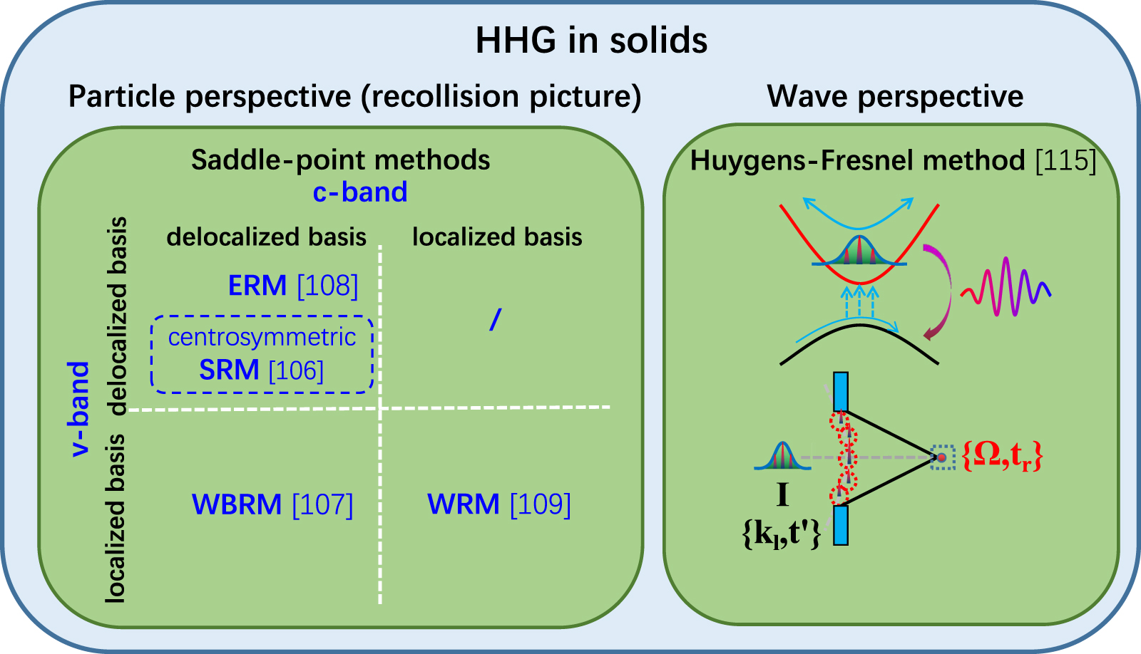
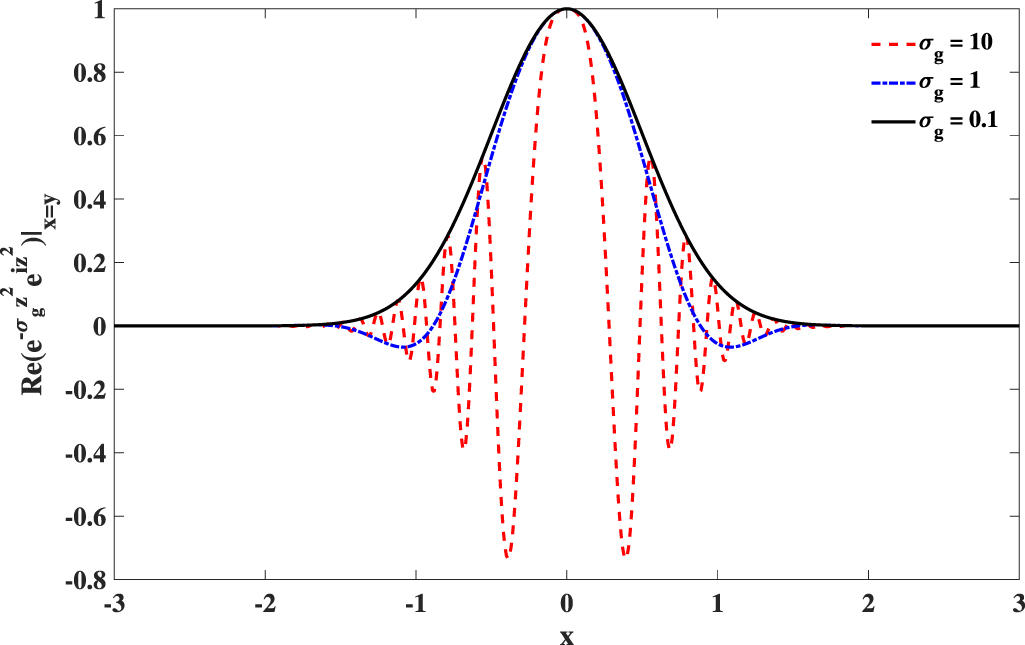
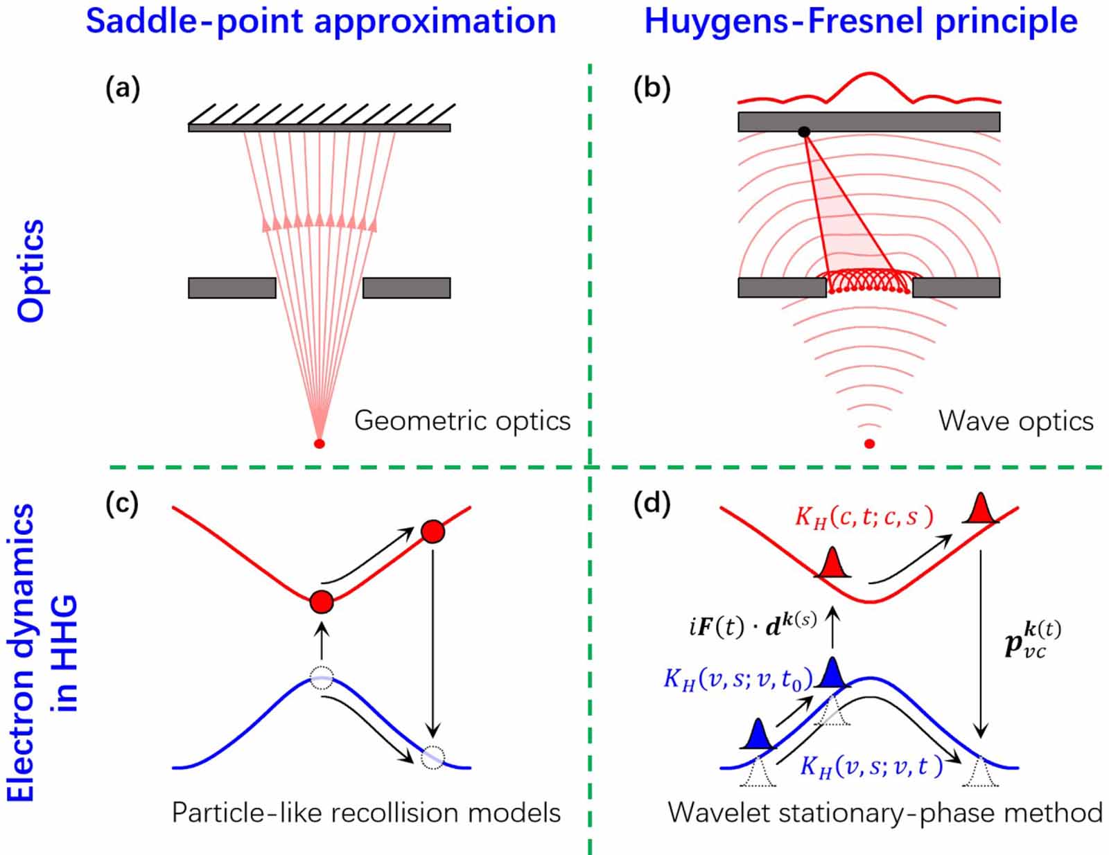
In this review, we focus mainly on the physical perspectives for HHG in solids, and the discussions are restricted to a two-band system under the single-active electron approximation. There are still many other complex effects, e.g. multiband effect [96–98, 110, 134–136], multielectron correlation effect [89, 91], propagation effects [99–103] and so on, which are under lively discussions and need further investigation. Strong field physics is a rapidly developing field. Its territory is also expanding rapidly, regarding both the involved laser parameters and species of materials. Possibly because of the big success of the particle-like recollision model in gas HHG, it is always simply extended to a new field and applications without strict thinking. The purpose of this review is to point out a problem which is often neglected in the process of expanding the application range of the present particle-like recollision theories and relevant technologies, that is, whether the original approximation or picture still works well. We hope that this review gives newcomers to get an overview of the topic and provides guidance on the potential development of theories and applications.
Acknowledgments
We acknowledge fundings from National Key Research and Developement Program (No. 2022YFA1604403) and National Natural Science Foundation of China (NSFC) (Nos. 91950202, 11934006, 12104172, 12225406, 12021004).
Data availability statement
No new data were created or analysed in this study.