the Creative Commons Attribution 4.0 License.
the Creative Commons Attribution 4.0 License.
 | 25 May 2023
Ten years of 1 Hz solar irradiance observations at Cabauw, the Netherlands, with cloud observations, variability classifications, and statistics
Wouter H. Knap
Chiel C. van Heerwaarden
Surface solar irradiance varies on scales down to seconds, and detailed long-term observational datasets of this variable are rare but in high demand. Here, we present an observational dataset of global, direct, and diffuse solar irradiance sampled at 1 Hz as well as fully resolved variability until at least 0.1 Hz over a period of 10 years from the Baseline Surface Radiation Network (BSRN) station at Cabauw, the Netherlands. The dataset is complemented with irradiance variability classifications, clear-sky irradiance and aerosol reanalysis, information about the solar position, observations of clouds and sky type, and wind measurements up to 200 m above ground level. Statistics of variability derived from all time series include approximately 185 000 detected events of both cloud enhancement and cloud shadows. Additional observations from the Cabauw measurement site are freely available from the open-data platform of the Royal Netherlands Meteorological Institute. This paper describes the observational site, quality control, classification algorithm with validation, and the processing method of complementary products. Additionally, we discuss and showcase (potential) applications, including limitations due to sensor response time. These observations and derived statistics provide detailed information to aid research into how clouds and atmospheric composition influence solar irradiance variability as well as information to help validate models that are starting to resolve variability at higher fidelity. The main datasets are available at https://doi.org/10.5281/zenodo.7093164 (Knap and Mol, 2022) and https://doi.org/10.5281/zenodo.7462362 (Mol et al., 2022); the reader is referred to the “Code and data availability” section of this paper for the complete list.
- Article
(2413 KB) - Full-text XML
- BibTeX
- EndNote


Clouds generate large intra-day surface solar irradiance variability, the spatiotemporal scales of which reach down to seconds or less (Yordanov et al., 2013; Tabar et al., 2014; Gueymard, 2017; Kivalov and Fitzjarrald, 2018), or tens of meters (Lohmann et al., 2016; Mol et al., 2023). Observing, understanding, and forecasting irradiance variability at these scales is important for a range of applications. Solar energy production and electricity grid stability is negatively affected by fast and local irradiance variability (Liang, 2017; Yang et al., 2022). Numerical weather prediction models are incapable of forecasting variability at these short scales; however, as the resolution of these models keeps increasing and sub-grid-scale irradiance variability parameterizations are developed, they require more detailed observations for validation. Cloud-resolving models and the development of more accurate 3D radiative transfer calculations in academic setups (e.g., Jakub and Mayer, 2015; Gristey et al., 2020; Veerman et al., 2022) likewise require detailed and accurate observations of solar irradiance. The heterogeneity of solar irradiance and the resulting surface fluxes is also an increasingly important topic in the field of land–atmosphere interaction (Helbig et al., 2021), with a nonlinear response of vegetation's photosynthesis for varying light intensities (Pearcy and Way, 2012) or diffuse irradiance penetration into canopies (Mercado et al., 2009; Durand et al., 2021).
Existing observational datasets of surface solar irradiance at the sub-minute scale are rare, in particular for multiple years or longer and with separate direct and diffuse irradiance measurements. Notable examples of such datasets include those used in previously mentioned studies (Tabar et al., 2014; Gueymard, 2017; Kivalov and Fitzjarrald, 2018; Lohmann, 2018; Gristey et al., 2020). In this work, we present such a dataset, which consists of 10 years of 1 Hz resolution global, direct, and diffuse irradiance, supplemented with meteorological observations for interpretation and data analysis. To the best of our knowledge, this is a unique observational dataset given its time span, temporal resolution, and multicomponent measurements. The separation of global horizontal irradiance (GHI) into direct and diffuse components is important for distinguishing and characterizing the different types of atmospheric conditions and specific conditions under which irradiance variability is generated. Most notably, the phenomenon of cloud enhancement, where clouds scatter additional sunlight to cloud-free spots on the surface to significantly increase total irradiance (Gueymard, 2017; Yordanov, 2015; Mol et al., 2023), is, by definition, a combination of direct and diffuse irradiance and cannot be understood with only GHI observations.
In this work, we will describe the 10-year observational dataset of solar irradiance, all supplementary meteorological observations and related processing, the time series variability classification algorithm, statistical datasets derived from all time series and classifications, and examples of how the data can be used. Sections 2 and 3 are a complete and more elaborate version of the condensed dataset description published in the Journal of Geophysical Research: Atmospheres (Mol et al., 2023).
All in situ observations in this dataset were taken at the Ruisdael Observatory in Cabauw (previously known as CESAR; https://ruisdael-observatory.nl/cabauw/, last access: 16 May 2023) of the Royal Netherlands Meteorological Institute (KNMI). The observatory, hereafter referred to as Cabauw, is located in a rural area in the southwest of the Netherlands (51.97∘ N, 4.92∘ E; Fig. 1a). The climate in the Netherlands is a typical ocean-influenced west coast climate, with relative mild and wet winters, despite the country's high latitude, and milder summers than further inland. KNMI provides an overview of the current Dutch climate and trends on their website (https://www.knmi.nl/klimaat, last access: 16 May 2023), including the long-term increasing trend in incoming solar radiation and recent extremes (e.g., that of spring 2020; van Heerwaarden et al., 2021). The following section describes all of the observational data that we used from Cabauw, the supplementary modeled clear-sky irradiance, the atmospheric composition reanalysis, the calculated solar positions, the satellite-derived cloud types, and the ground-based cloud cover.
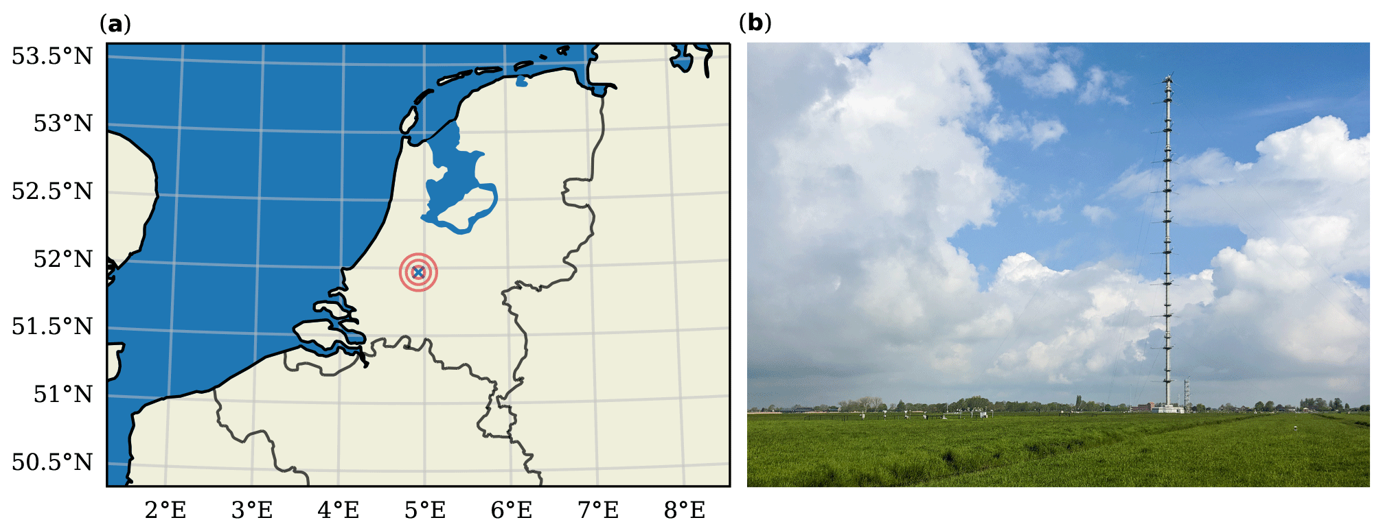
Figure 1Ruisdael Observatory, Cabauw, the Netherlands, where all of the observations in our dataset took place. In panel (a), the geographical location is marked with a cross, and the circles are the 5–15 km radii for satellite cloud-type extraction. A photograph of the 213 m high tower at the Cabauw site, with the BSRN station among other instruments in the bottom left, is shown in panel (b).
2.1 Surface solar irradiance observations
The surface solar irradiance station at Cabauw is part of the Baseline Surface Radiation Network (BSRN; Driemel et al., 2018), which has been operational since 2005. The BSRN station measures all components of the surface radiation balance. Observations are logged at a 1 Hz frequency, reprocessed to 1 min quality-controlled and validated data, and made available publicly on the PANGAEA data repository (Knap, 2022) along with instrument metadata; the station is maintained by station scientist Wouter Knap (KNMI). While a 1 min resolution is enough for many applications, in particular those concerned with the surface net radiation balance at longer timescales, much of the cloud-driven irradiance variability occurs at sub-minute scales. For the purpose of research into cloud-driven irradiance variability at these short timescales, a separate 10-year subset of solar irradiance at a 1 Hz resolution has been released (Knap and Mol, 2022) and is described here. This subset spans from February 2011 to December 2020. The three components are global horizontal irradiance (GHI) and diffuse irradiance (DIF), measured with Kipp & Zonen CM22 pyranometers, and direct normal irradiance (DNI), measured with a Kipp & Zonen CH1 pyrheliometer.
2.1.1 Sensor response time and resolved variability
The pyranometer and pyrheliometer instruments are thermopiles, meaning that there is a nonzero response time to variations in incoming radiation, i.e., the time it takes for the thermopile to adjust to changes in irradiance signal. Thus, the true resolved resolution is not 1 Hz, although whether or not this impact is noticeable depends on the magnitude and rate of change in irradiance variability. According to the manufacturer's specifications, the CH1 pyrheliometer has a 7 s (95 %) or 10 s (99 %) response time (Kipp & Zonen, 2001), whereas these values are 1.66 s (66 %) or 5 s (95 %) for the CM22 pyranometers (Kipp & Zonen, 2004). This results in a likely underestimation of variability at 1 Hz, but the exact extent of this underestimation is hard to quantify given the absence of solar irradiance measurements with fast-responding sensors at a similar location as well as the lack of measurements that are long enough to sample diverse weather conditions. Figure 2 illustrates the power spectral density (PSD) of a year of BSRN 1 Hz data. Tabar et al. (2014) present spectra (their Fig. 2) for 1 year of data from a semiconductor pyranometer (with a >1 Hz response time) that show an order of magnitude higher PSD at 1 Hz compared with 0.1 Hz, as in our Fig. 2. However, these data were collected in Hawaii, which is a very different geographical location and climate compared with Cabauw. Alternatively, 2 weeks of summer time 10 Hz irradiance observations from fast radiometers (Mol and Heusinkveld, 2022) show a steeper decline between 0.1 and 1 Hz than the BSRN data. This supports the idea that the true cloud-driven irradiance variability does not always extend towards 1 Hz and higher frequencies and that the slow response time often has no noticeable effect.

Figure 2Power spectral density of 1 year (2016) of 1 Hz BSRN data (GHI component). The 1 min spectrum is based on resampled 1 Hz data. As a reference, scaling is added to emphasize the steep decline after 0.1 Hz towards 1 Hz. An additional comparison is shown for the spectrum from a semiconductor radiometer deployed during the FESSTVaL (Field Experiment on submesoscale spatio-temporal variability in Lindenberg) campaign from 14 to 30 June 2021 near Berlin, Germany.
Based on the technical specifications of the pyranometer and pyrheliometer, we are at least confident that variability is resolved up to 0.1 Hz (10 s). This is also supported by van Stratum et al. (2023), who showed agreement between the BSRN dataset presented in this paper and irradiance spectra from semi-realistic large-eddy simulation up to 0.1 Hz (their Fig. 6). Given the uncertainty regarding how much of the true variability is resolved between 0.1 and 1 Hz, we advise analyses at 1 Hz only in combination with additional constraints, such as knowledge of cloud properties and their velocity, to estimate the fastest possible changes in irradiance. For example, in Mol et al. (2023), knowledge of wind speed, cloud size distributions, and cloud edge transparency were combined to utilize the data down to 1 Hz.
One last implication is that the slow response time slightly reduces the contrast in data. Ehrlich and Wendisch (2015) demonstrated a reconstruction technique of the true 1 Hz signal through deconvolution, essentially a sharpening technique, which is not a trivial exercise. We have not applied this here, as we cannot validate if it works reliably for our dataset, but we mention it as an option to anyone who might want to attempt to apply the method despite its challenges. The only preprocessing that we apply to the data, namely gap filling and quality control, is discussed in Sect. 3.1.
2.2 Supplementary irradiance data
2.2.1 Solar position and direct horizontal irradiance
Information about the Sun's position is important for quality control, data analysis, and interpretation of results. Calculations of the Sun's position (elevation and azimuth angle) are done using the Pysolar (https://github.com/pingswept/pysolar, last access: 16 May 2023) Python package at a 1 min resolution, linearly interpolated to 1 s. For the purposes of this research, the calculations are indistinguishable from highly accurate peer-reviewed code such as the Solar Position Algorithm (SPA; https://midcdmz.nrel.gov/spa/, last access: 16 May 2023). Using the solar elevation angle α (degrees above horizon, or as a zenith angle), we calculate the horizontal component of direct irradiance: DHI = DNI ⋅ sin(α). An alternative calculation is DHI = GHI − DIF, which (in the case of a good measurement setup) should be equal to DNI ⋅ sin(α) and is the basis for one of the checks in data quality control (discussed in Sect. 3.1).
2.2.2 Clear-sky irradiance and atmospheric composition
Clear-sky global horizontal irradiance (GHIcs) is the total downwelling horizontal solar irradiance in the absence of clouds. We use Copernicus Atmosphere Monitoring Service (CAMS) McClear version 3.5 (released in September 2022; Gschwind et al., 2019) as the GHIcs reference for our dataset. CAMS McClear includes corrections based on atmospheric composition reanalysis, such as aerosols and total column atmospheric water vapor. This allows us to define times when GHI exceeds GHIcs only through the effect of clouds as best we can, as opposed to simpler techniques that do not correct for aerosols and chemical composition. Atmospheric composition input for McClear is included in their publicly available dataset (https://www.soda-pro.com/web-services/radiation/cams-mcclear, last access: 16 May 2023), which we add to our dataset for context. The only further processing applied to these data is linear interpolation from 1 min to 1 s to match the irradiance observations.
2.3 Additional in situ measurements
2.3.1 Wind profiles from Cabauw
A 213 m high tower provides wind speed and direction measurements at 2, 10, 20, 40, 80, 140, and 200 m above ground level at a 10 min intervals (Wauben et al., 2010). Figure 1b shows the tower with respect to the BSRN site, which is a few hundred meters to the south. We apply no further processing to these data, apart from creating daily files from the monthly files. The original tower data (including temperature, visibility, and humidity) are shared publicly by the KNMI on their open-data platform: https://dataplatform.knmi.nl/dataset/cesar-tower-meteo-lb1-t10-v1-2 (last access: 16 May 2023).
2.3.2 NubiScope
To obtain detailed cloud cover observations for analysis, validation of satellite observations (Sect. 2.4), and irradiance-based sky-type classification (Sect. 3.3.2), we use the NubiScope located within a few meters of the BSRN instrumentation (Wauben et al., 2010). In 10 min, this instruments makes a hemispherical scan of the sky using infrared sensors to determine the cloud fraction and various categories of sky type. For validation and analyses purposes, we focused on a 3-year subset (2014–2016) of NubiScope data. If necessary, additional data (May 2008 to April 2017) are publicly available at https://dataplatform.knmi.nl/dataset/cesar-nubiscope-cldcov-la1-t10-v1-0 (last access: 16 May 2023). Again, we applied no further processing, apart from turning monthly files into daily files.
2.4 Satellite observations
The CLAAS-2 (CLoud property dAtAset using SEVIRI, Edition 2; Benas et al., 2017) satellite product provides cloud cover, cloud-top pressure (CTP), and cloud optical thickness (COT) every 15 min during daytime at an approximate spatial resolution of 20 km2 over Cabauw. We provide 3 years of satellite data (2014–2016) for both validation and cloud-type analyses, and the post-processing steps for these data are described in Sect. 3.2.1.
3.1 Quality control and completeness of irradiance data
One of the first steps in the processing is constructing daily files from the raw instrument data, which are occasionally missing a few seconds of information. In such cases, we apply linear gap filling between measurement points, after which we apply quality control and derive all other variables. Gap-filled data points are not flagged. Data quality control for the irradiance measurements is necessary to mask out station maintenance, malfunctioning instruments, or other cases of bad data, such as those caused by precipitation. Maintenance occurs on alternate days (Monday, Wednesday, and Friday) to ensure that the high BSRN quality standards are met, and it is the most common source of anomalous measurements. It is typically brief and only involves sensor cleaning, although sometimes instrumentation is disabled or replaced due to quality issues such that there are gaps of hours up to a few days. For the official 1 min BSRN dataset (Knap, 2022), all measurements during such periods are filtered. The 1 Hz version includes quality flags (“good” or “bad” data) derived from the official dataset, where good denotes that all three components (GHI, DNI, and DIF) are valid. The 1 Hz version includes the original measurements, and quality flags have to be applied to filter bad data; therefore, the user can decide on the strictness of filtering themselves. We independently determined data quality at the 1 Hz level by performing the following checks (which are the result of a trial-and-error process through manual data inspection):
-
The absolute rate of change in the DIF and DNI components with respect to clear sky between two consecutive measurement points (2 s) has to be below 5 % and 20 %, respectively.
-
The absolute rate of change in the GHI component with respect to clear sky between two consecutive measurement points has to be below 5 % for cloudy conditions and 20 % for sunny conditions. This leads to some false positives, which are reset if GHI and DHI changes are well correlated.
-
Invalid measurements are padded by 180 s before and after to be on the safe side.
-
The residuals ΔQabs = and ΔQrel = ⋅ have to be below 10 % and 20 W m−2 for a 15 min time frame, respectively. This time frame is necessary because the instruments are a few meters apart, which leads to a decorrelation of the individual components and larger residuals with decreasing timescales.
-
To be flagged as good quality, all three components have to pass the tests. If one or more components include missing or bad data, the data for that time are considered bad.
The implementation of these rules is outlined in the published processing code (see Sect. 5) and can be modified to adjust the strictness of the quality control. There are only minor differences between the custom quality flags based on the 1 Hz data and the official 1 min BSRN dataset flags. For all data during daytime (solar elevation angle above 0∘), 97.98 % of the flags are similar between the custom and official quality flags, 1.26 % are bad with respect to the custom flags but good with respect to the official flags, and 0.77 % are good with respect to the custom flags but bad with respect to the official flags. Most of these mismatches originate from just a few days, and the resulting data are otherwise in very close agreement, with the vast majority of data being of good quality. Figure 3 illustrates the data availability after (custom) quality control for the whole 1 Hz dataset and shows that most months and years have almost 100 % complete and good data for all three measured irradiance components. As proof of the data quality, Fig. 9 illustrates that DIF + DHI = GHI after quality control for every month of the year. The minor negative bias of DIF + DIR that is visible for some months is within a range of 0.3 %–0.6 %, which far exceeds the constraints imposed by the official BSRN standard. These residuals are deemed insignificant and have no implications for the use cases of this dataset, as these concern irradiance variability.

Figure 3BSRN Cabauw 1 Hz data availability per month of available years, during daylight (solar elevation angle above 0∘), after custom quality control. Numbers are rounded off percentages.
3.2 NubiScope and satellite processing
The NubiScope and satellite data are used as a validation dataset for irradiance-derived sky types (described in Sect. 3.3) and to provide observations of clouds and sky type for data analysis. Here, we describe the processing applied to the cloud observations as well as how the validation dataset was created.
3.2.1 Satellite processing
We classify cloud types using a simple cloud-top pressure (CTP) and cloud optical thickness (COT) categorization (see the International Satellite Cloud Climatology Project, ISCCP, algorithm description in NOAA, 2022, their Fig. 20). The nine cloud types are cumulus (Cu), stratocumulus (Sc), and stratus (St) for low-level clouds; altocumulus (Ac), altostratus (As), and nimbostratus (Ns) for mid-level clouds; and cirrus (Ci), cirrostratus (Cs), and cumulonimbus (Cb) for high-level clouds. Cu, Ac, and Ci are the optically thinnest clouds for each altitude, and St, Ns, and Cb the thickest; as the only exception in this list, Cb spans from low to high altitude. In this study, we used the abovementioned classification to group cloud conditions of various altitudes and optical thicknesses together in a more intuitive way, although analyses can be done on the input COT and CTP data rather than the derived cloud types. The main limitations are that both the cloud fraction and actual cloud optical thickness contribute to a higher reported optical thickness in a satellite pixel, which is a result of limited spatial resolution, and higher clouds can obscure lower clouds. The spatial satellite product is converted to a time series representative of the BSRN station by determining the most common cloud class within a 5, 10, or 15 km radius of Cabauw, as illustrated by the circles in Fig. 1a. A smaller radius is not possible due to satellite resolution (pixel area of ≈20 km2), and larger radii become unrepresentative for Cabauw. Cloud cover is derived by calculating the fraction of pixels with clouds within a given radius, which is likely an overestimation due to sub-pixel cloud fractions not always being 1. However, overall agreement with the NubiScope is not bad, as illustrated by the similar probability densities in Fig. 4. Correlation coefficients between the two only show marginal improvement between 10 and 15 km. The satellite-derived cloud cover overestimates the extremes at [0.0–0.1) and [0.9–1.0] compared to values bins of [0.1–0.2) and [0.8–0.9), and it does not have the nuances that the NubiScope can resolve. For r=5 km, there are only four pixels, so cloud cover from this is too coarse for most applications, but the dominant cloud type derived from this narrow area around Cabauw is expected to be most representative. This might change for high-altitude clouds at low solar elevation angles, for example, and may perhaps require more sophisticated approaches; therefore, we have included the original spatial satellite fields in our dataset.
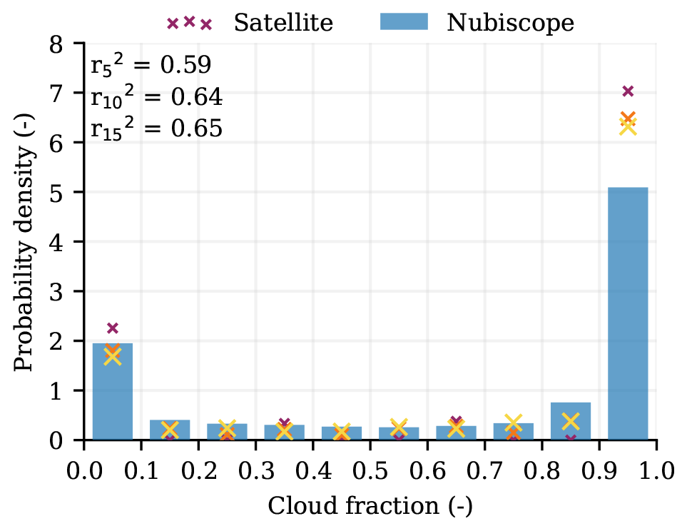
Figure 4Comparison of the cloud fraction derived from satellite to the ground-based NubiScope. The analysis is done for radii of 5, 10, and 15 km and shows the probability density for 10 bins with cloud fractions between 0 and 1. Satellite radii range from 5 km (dark, small) to 15 km (light, large), and are shown using the cross markers. Correlation coefficients are shown in the top left for each radius. Data range from January 2014 to December 2016 and are interpolated (using nearest-neighbor interpolation) to a common 5 min time axis.
3.2.2 Validation dataset
Employing the clear-sky and overcast classifications based on a combination of the NubiScope and satellite data, we derive a validation dataset to be used for statistical verification of sky types based on irradiance observations (Sect. 3.3.2). Because both instruments have their limitations, the idea is to only identify a situation as clear sky or overcast if both datasets are in agreement. The rest of the preprocessing involves interpolation to a common 1 min resolution grid, and we also mask out data if either of the two products is missing for given a given time. The validation dataset is provided in Mol et al. (2022) for all three radii, although we mostly use r=10 km, for the years 2014 to 2016. Disagreement between the two observational datasets is common, with the NubiScope being roughly 3 or 1.5 times more conservative with respect to classifying a sky type as clear or overcast, respectively. This is likely not only to do with the difference in the type of observation (ground-based versus remote sensing) but is also due to the fact that the NubiScope is a more sensitive instrument, as we illustrate in Fig. 4 and discuss in Sect. 3.2.1. In most cases, the NubiScope is more conservative; thus, both the clear-sky and overcast conditions are mostly controlled by what the NubiScope sees. Figure 8 illustrates this best, with the satellite and NubiScope differing with respect to the seasonal cycle for clear-sky conditions and with respect to yearly averages for both clear-sky and overcast conditions.
3.3 Irradiance classifications
The main addition to the core 1 Hz irradiance time series is the classification of measurements into various categories that describe the type of irradiance variability. We calculate two sets of classification types: one instantaneous classification to qualify a single measurement point and one more indirect classification to qualify the sky type based on longer time frames. First, we describe what the classifications represent and how they are calculated; we then outline how they are further processed to derive a wide range of interesting statistics about irradiance variability. Examples are shown in Figs. 5, 6, and 7, and the public dataset (Mol et al., 2022) includes similar quicklooks for all 10 years of the time series.
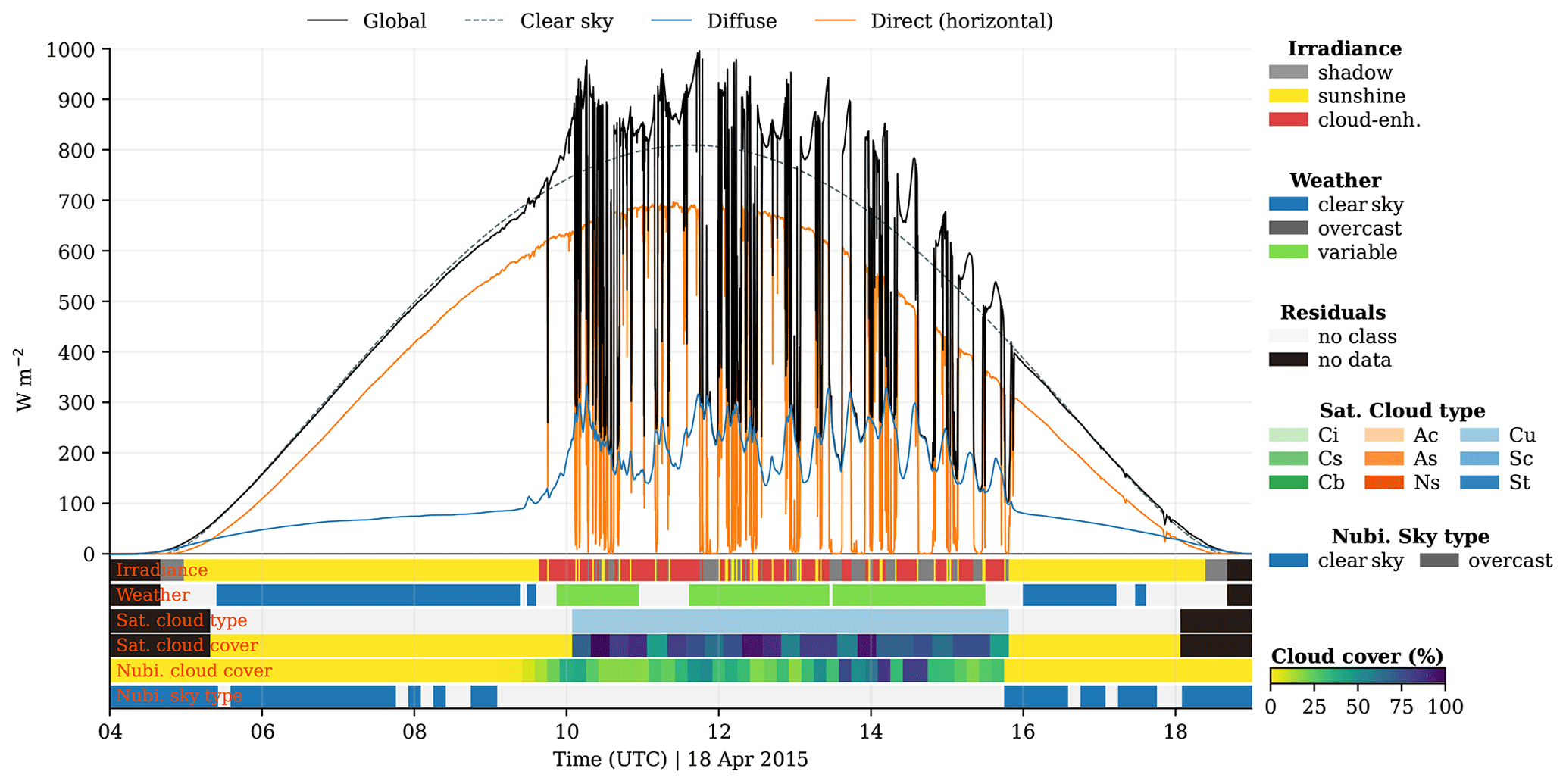
Figure 5Surface solar irradiance time series at 1 Hz, irradiance classifications, and cloud observations for 18 April 2015. The time series starts with clear-sky conditions and becomes highly variable with respect to surface irradiance due to scattered boundary layer clouds. The three measured irradiance components – global, diffuse, and direct horizontal irradiance – are shown together with modeled (CAMS McClear) clear-sky irradiance.

Figure 6Surface solar irradiance observations of a mostly overcast day (3 April 2015), with a similar layout to Fig. 5. The satellite and NubiScope observations indicate overcast conditions with mostly opaque mid- to high-level clouds (As or Cs), although there are brief periods of partially transparent clouds (Ac).
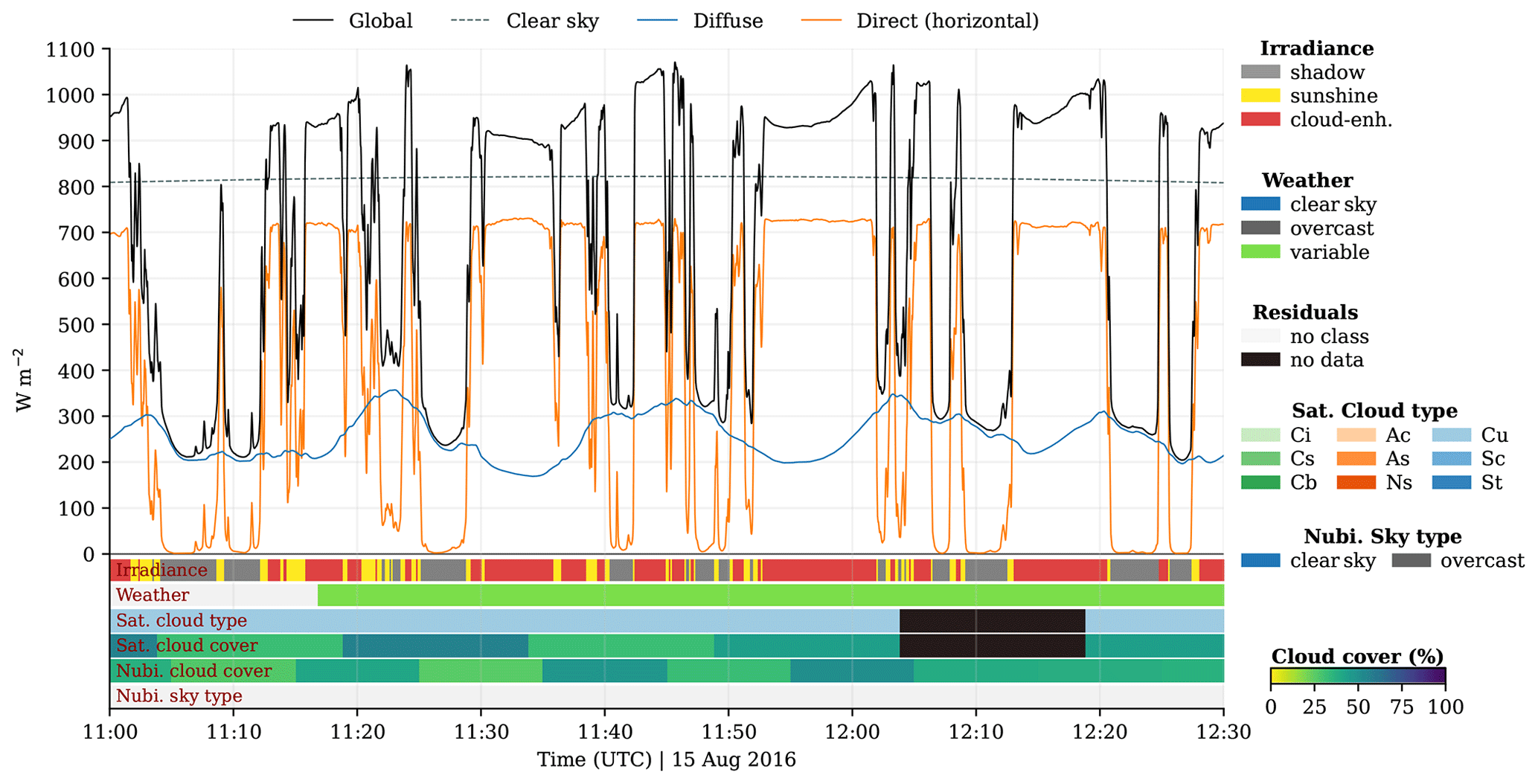
Figure 7Detailed example of cloud-driven irradiance variability. Similar to Fig. 5 but for 90 min on 15 August 2016.
3.3.1 Cloud shadow and enhancement
Broken cloud fields making patterns of cloud shadows and cloud enhancements are one of the most noticeable drivers of intra-day irradiance variability (e.g., Yordanov et al., 2015; Gueymard, 2017; Veerman et al., 2022). Cloud shadows occur when (most) direct irradiance is blocked, and cloud enhancement occurs when light scattered by clouds locally coincides with direct irradiance to increase global horizontal irradiance above clear-sky values. We define a shadow as a region where direct normal irradiance (DNI) is below 120 W m−2, which is the inverse of what the World Meteorological Organization (WMO) defines as sunshine (DNI ≥ 120 W m−2; WMO, 2014), as this is a straightforward implementation. Cloud enhancement requires a more careful approach. We define the occurrence of cloud enhancement, using a single measurement, as when the global horizontal irradiance (GHI) exceeds the reference clear-sky irradiance (GHIcs). In reality, observed GHI can still fluctuate noticeably under cloud-free conditions, and the GHIcs reference may not be perfect; therefore, there is some uncertainty in the detection for weak cases of cloud enhancement. To prevent false positives in the detection algorithm, we first apply an activation threshold defined by the GHI exceeding GHIcs by 1 % and 10 W m−2. Both a relative and absolute threshold are used, as clear-sky irradiance ranges from 100 to 103 W m−2 as function of the solar elevation angle (i.e., time of day). A value of 10 W m−2 is based on 1 % of the typical order of magnitude for clear-sky irradiance around noon for Cabauw. When the threshold is reached, adjacent measurements are also marked as “cloud enhancement” as long as they exceed GHIcs by 0.1 %. Edge cases at low solar elevation angles are removed by requiring the DNI to be at least 10 W m−2. All of these thresholds are chosen to enable us to capture all but the weakest of cloud enhancements, which are arguably not important. The residual third class is called “sunshine” and is based on the WMO definition of sunshine minus cloud enhancement. Detection criteria can be adjusted in the code and recalculated, or another level of filtering can be applied after classification through the derived event statistics (discussed in Sect. 3.4). Examples of the classifications are shown in the top color-coded bar beneath the time series in Figs. 5, 6, and 7.
3.3.2 Overcast, clear-sky, and variable irradiance
The second group of classifications represents the irradiance “weather” type, or sky type, based on irradiance data only. The weather types are clear sky and overcast for smooth and predictable surface irradiance, and a third class of “variable” irradiance represents pronounced and unpredictable 3D radiative effects to contrast the former two. The way that these classifications are derived is partially based on subjective thresholds and assumes good-quality clear-sky data; thus, we validate against satellite and ground-based cloud cover observations.
Table 1Skill scores for irradiance-based sky-type classifications compared to the validation dataset (satellite + NubiScope). Scores are based on a contingency table approach. POD is the probability of detection and FAR is the false alarm ratio.
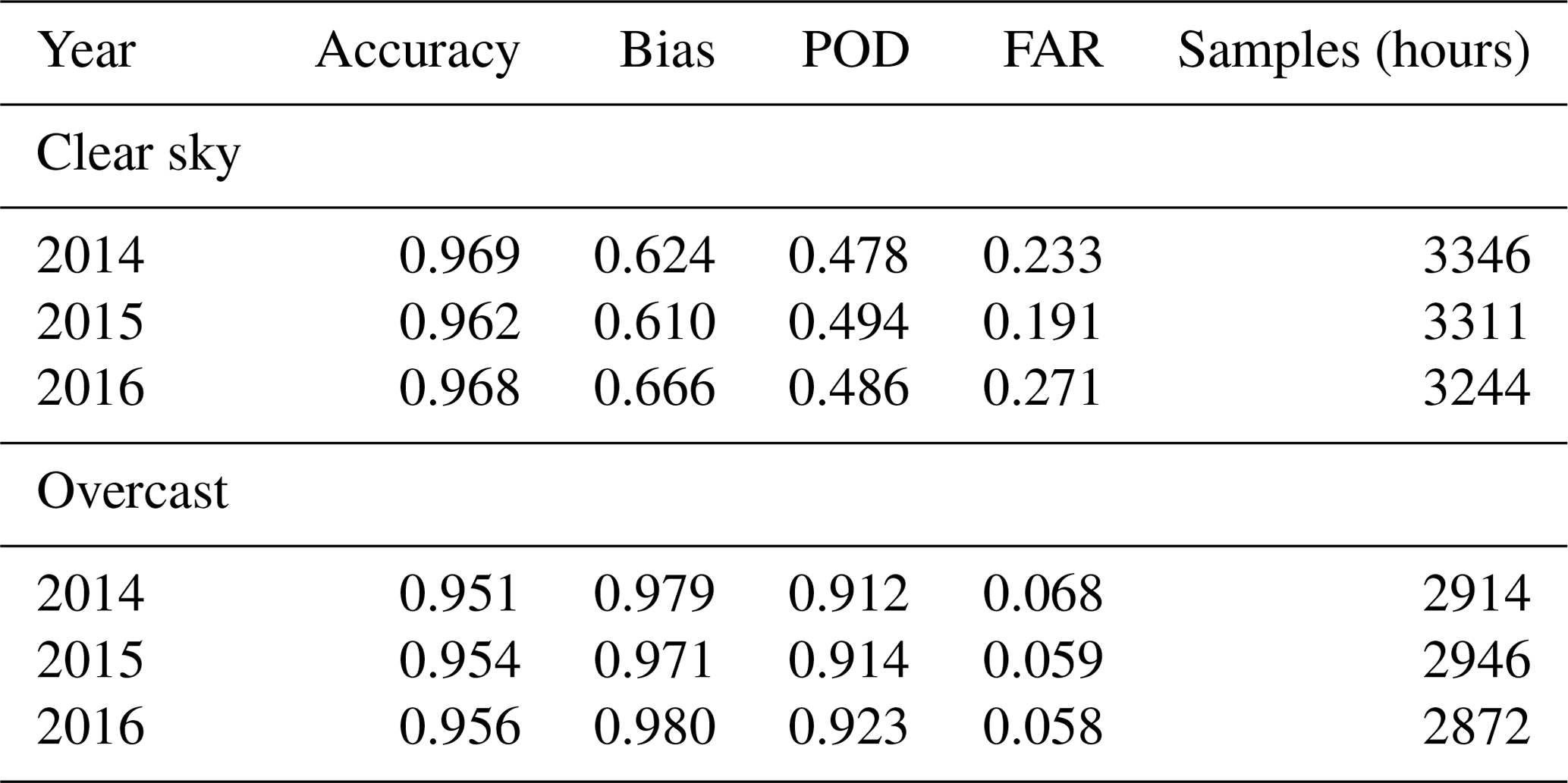
We classify those points in the time series for which GHI stays within 3 % or 5 W m−2 of GHIcs in a 15 min centered moving window, with a maximum standard deviation of the ratio within that window, as clear sky. This irradiance-based algorithm emphasizes smoothness, and thus predictability, more than exactly matching GHIcs, so as to not rely too much on CAMS McClear being perfectly accurate. Clear-sky conditions are uncommon, occurring between 5 % and 15 % of the time depending on the observational method (Fig. 8). Skill scores indicate that the irradiance-based classification misses almost half of the cases (probability of detection close to 50 %) and is generally too conservative (bias <1) with respect to the validation dataset (see Table 1). The negative bias against the validation dataset, which is not what Fig. 8 shows, is due to the skill scores only being calculated for cases in which there is agreement between the satellite and NubiScope, rather than for all available data in Fig. 8. The order of magnitude of occurrence is similar to what the validation dataset suggests, but the seasonal cycle is not reproduced, although seasonality between the irradiance classification and satellite alone is similar. For 2014 and 2015, the seasonal correlation to the NubiScope is also much better, but there were many cases in 2016 where the NubiScope saw thin cirrus (cloud cover < 5 %, 17, 18, 23, 24, and 25 August) rather than clear sky. In all of these cases, GHI < GHIcs, which is consistent with thin cirrus attenuating incoming solar radiation slightly; these instances are not part of the validation set due to disagreement between satellite and NubiScope measurements. It appears (from Table 1 and Fig. 10) that there is poor skill in the irradiance-based classification, although manual inspection of quicklooks gives a different impression and most of the bias shown in Fig. 10 appears to stem from cases with thin cirrus. If one wants to filter out the thin-cirrus cases, the classification threshold can be made more strict, thereby limiting cases to more true clear-sky conditions. Figure 6 shows a case with overall agreement between the NubiScope-, satellite-, and irradiance-based clear-sky classifications. We refer the reader to the public dataset (Mol et al., 2022) with time series quicklooks for many more examples.
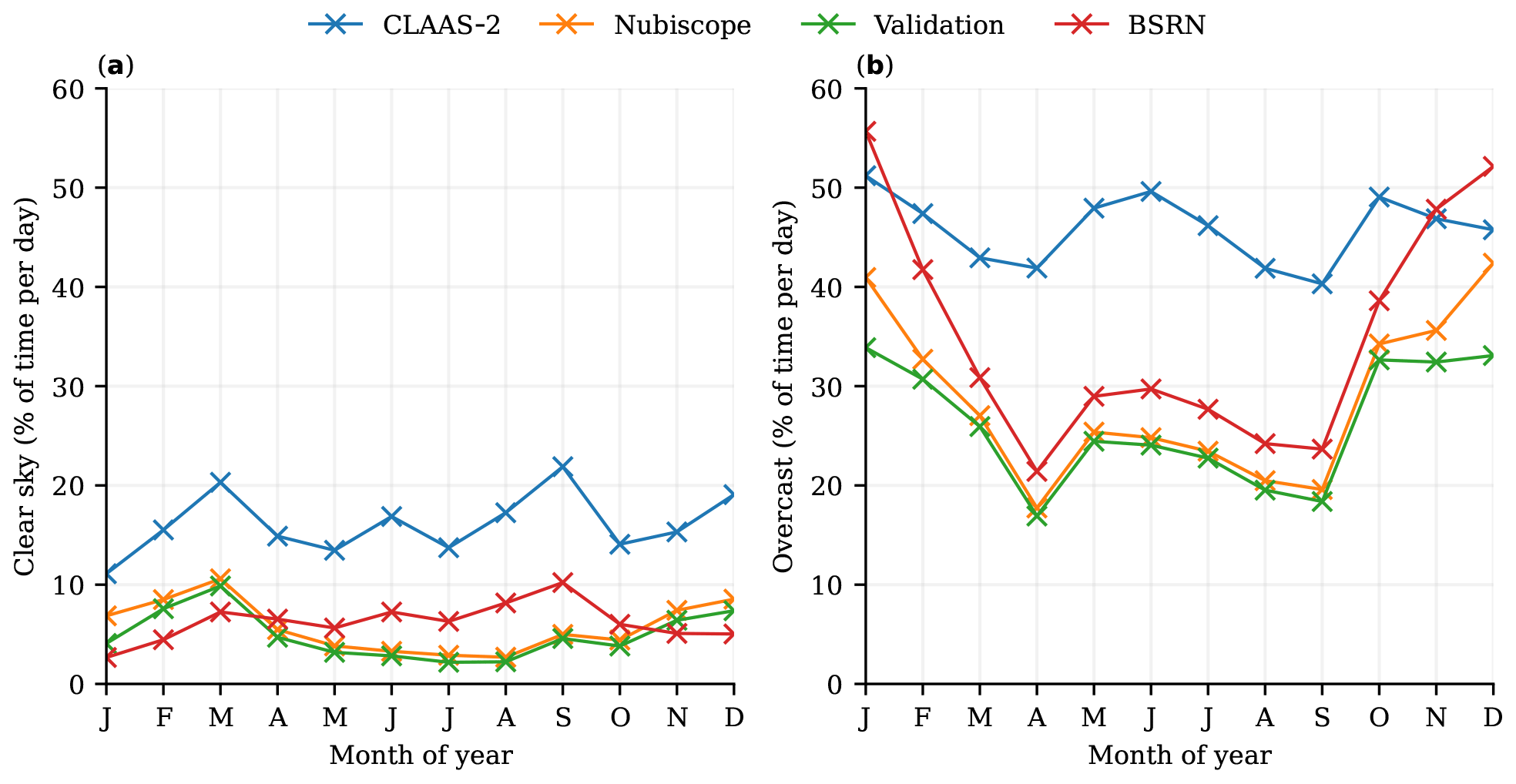
Figure 8Comparison of sky-type classifications based on satellite time series (r=10 km), NubiScope, and 1 Hz irradiance observations. The validation period is from 2014 to 2016, in units relative to available data during daylight (solar elevation angle α>0∘).
We define overcast weather as a period of 45 min during which the sum of DNI is below 1 % of GHIcs and the average is below 10 W m−2 (in order to catch rare edge cases). This class is indicative of continuous, optically thick, and persistent cloud cover, which is a common occurrence in the Netherlands (20 %–50 % of the time depending on the season), and it does well against the validation dataset. The probability of detection is high (92 %), with 6 % false alarms and only a slight negative bias of −1.7 %. Scores move slightly toward a positive (+2.6 %) or negative (−5.1 %) bias when shortening or lengthening the moving window to 15 and 60 min, respectively. Although a cloud cover of 100 %, as seen by the NubiScope and satellite, is classified as overcast in the validation dataset, cloud cover does not imply that the optical thickness is high enough to block all direct irradiance. This distinction is illustrated in Fig. 6, which shows good agreement for overcast conditions overall, although there is still some irradiance variability with 100 % cloud cover around 10:00 UTC. This example emphasizes our definition of overcast as smooth and predictable diffuse irradiance weather, as opposed to a sky type with 100 % cloud cover. The seasonal cycles between the irradiance-based sky type and NubiScope correlate well (Fig. 10), whereas the satellite yearly cycle is less pronounced.
Finally, the variable weather class, which is built upon the instantaneous classifications defined in Sect. 3.3.1, is defined as any 60 min window in which 10 transitions from a shadow to cloud enhancement or vice versa occur. It is indicative of weather associated with a characteristic bimodal distribution of irradiance, cloud enhancements, and at least a handful of large fluctuations in a short time frame, all of which current numerical weather prediction models cannot reproduce. This classification does well with respect to locating highly variable irradiance conditions, examples of which are shown in Figs. 5 and 7, and can, for example, be used to find case studies.
3.4 Event statistics
Within the classified irradiance time series, we call sections of cloud enhancements or shadows “events”. The 10 years of irradiance time series contain 184 447 cloud shadows and 186 685 cloud enhancement events. For every event, the start and end time are used to select complementary radiation and meteorological data, such that every cloud enhancement and shadow event can be characterized. Notable examples are statistics of event duration, maximum cloud enhancement strength, minimum direct irradiance “min(DNI)”, mean 200 m wind speed, dominant cloud type, maximum cloud-top height, and mean solar elevation angle. Event statistics such as these allow for the filtering of events according to additional criteria, e.g., comparing events of different magnitudes or finding the most extreme cases of cloud enhancement for a given cloud type. Event statistics for cloud shadows and enhancements are included in the public dataset (Mol et al., 2022).
3.5 Daily statistics
For case study selection or climatological overviews, we calculate daily statistics, which are mostly aggregates of irradiance and classification data. This statistic file is included in the public dataset. We use this to create figures, such as Figs. 3, 9, and 10, and to find specific case studies, as detailed in Table 2.
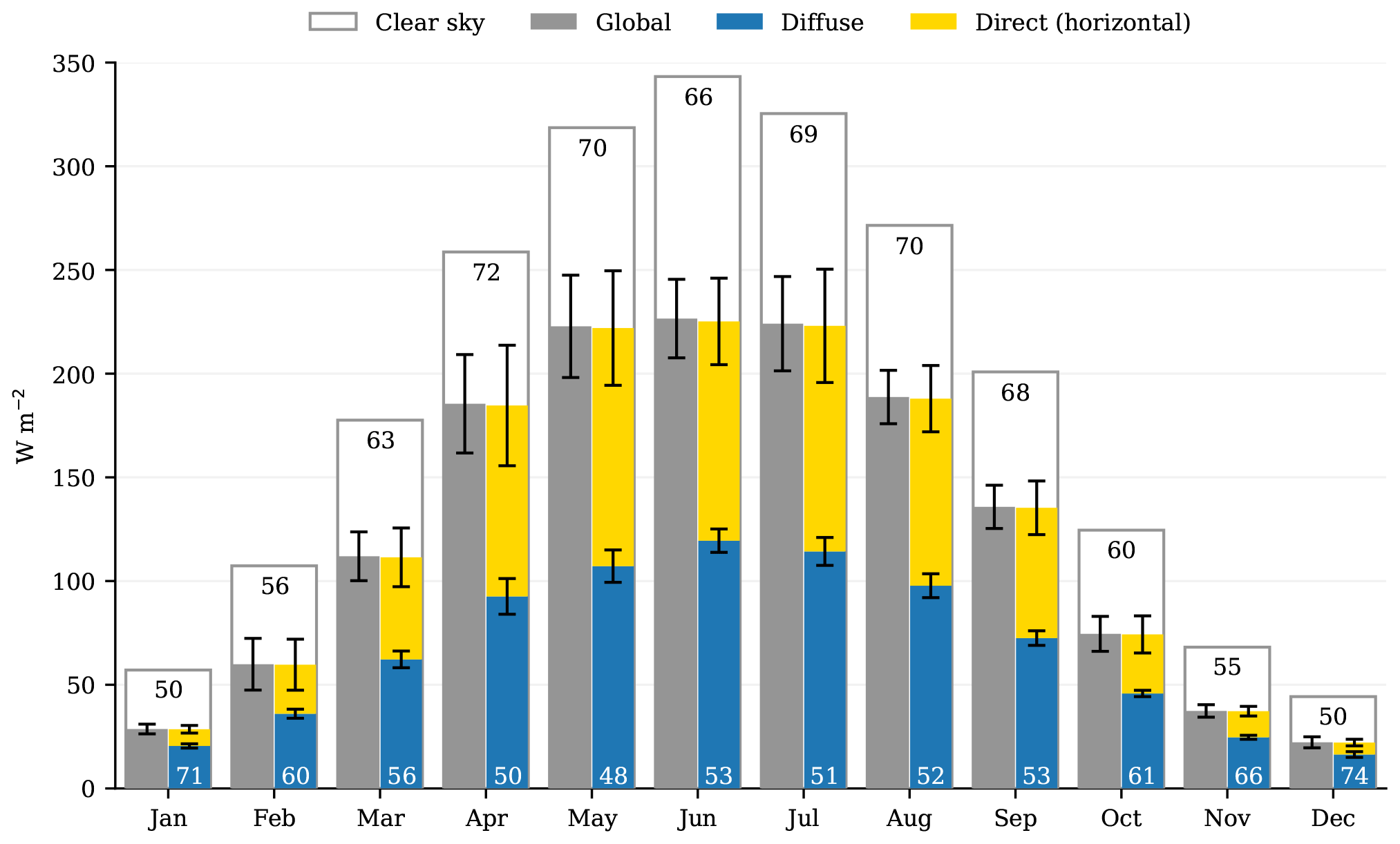
Figure 9Surface irradiance climate for the period from February 2011 to December 2020 based on the 1 Hz dataset of all three components. The numbers at the bottom indicate the percentage of diffuse irradiance (DIF) to global horizontal irradiance (GHI). The error bars indicate the year-to-year standard deviation for each component. The white bars encompassing the three components show the clear-sky irradiance (GHIcs) for each month, based on CAMS McClear, where the numbers at the top are the percentage of GHI compared with GHIcs. Only days with >95 % data completeness are included.
The following section provides some examples and (potential) use cases of the dataset, including previously completed work. Veerman et al. (2022) and Tijhuis et al. (2022) research 3D radiative transfer modeling approaches for cumulus case studies, where 1 Hz irradiance time series and statistics are used as validation. In Mol et al. (2023), we show how the spatiotemporal scales of cloud shadows and enhancements are described by power laws and driven by cloud size distributions, using the event statistics as described in Sect. 3.4.
Figures 9 and 10 give an overview of the seasonal and yearly variability in solar irradiance and its classifications that characterize the midlatitude climate of Cabauw. Figure 9 also partially serves as validation of the BSRN instrumentation, with the direct and diffuse components summing to the GHI, as should be the case. Figure 10 illustrates the typically overcast conditions during winter and the highly variable irradiance conditions during summer, with significant year-to-year variability.
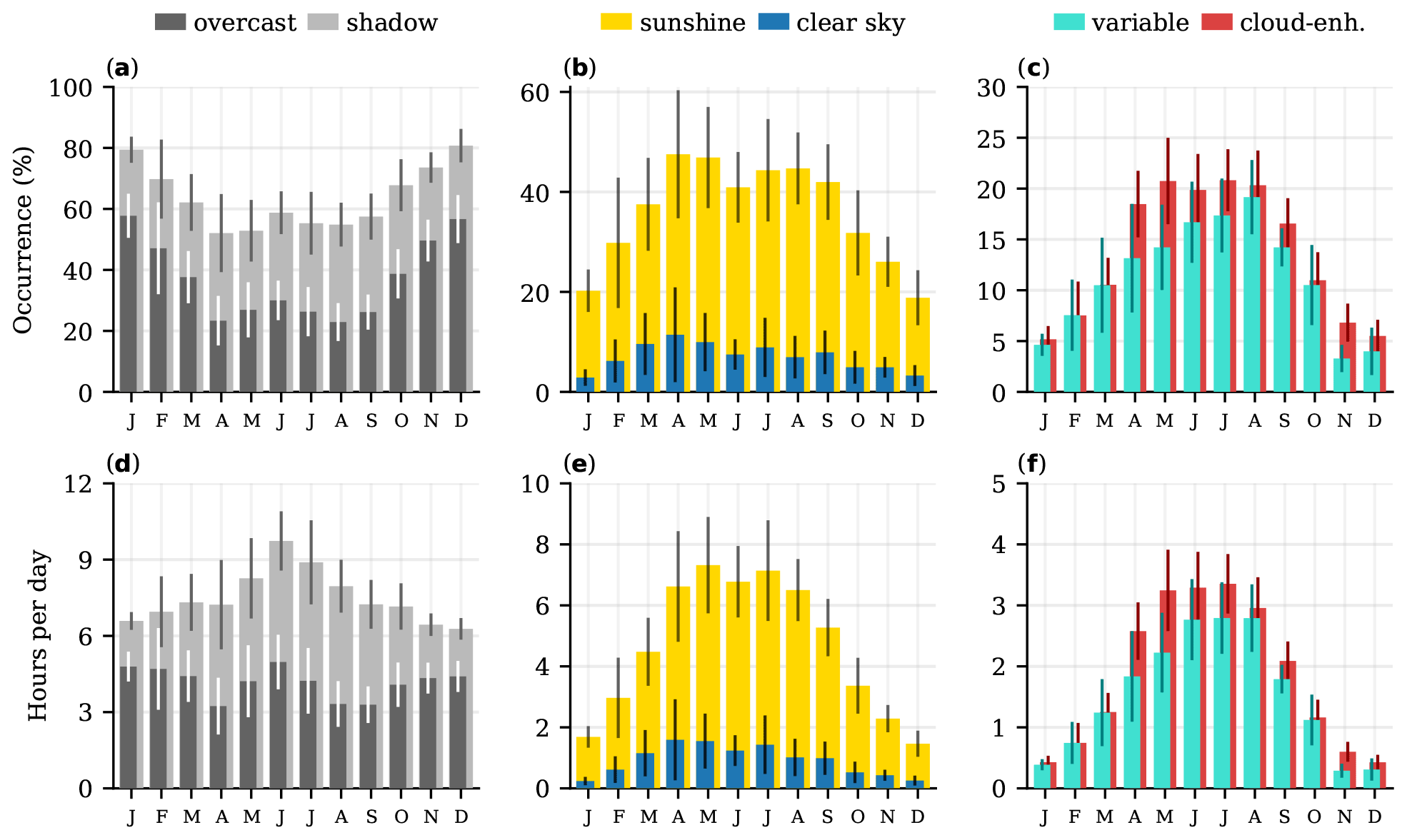
Figure 10The instantaneous and weather classification, with respect to the occurrence per month, showing the relative (a–c) and absolute (d–f) climatology of each classification throughout the year for all available data (February 2011 to December 2020). Here, sunshine also includes the portion marked as cloud enhancement, such that shadow + sunshine = 100 %. The reader is referred to Sect. 3.3 for the six classification definitions shown here. The relative occurrence is expressed as a percentage of daylight (solar elevation angle > 0∘), and the absolute occurrence is expressed in average hours per day. Error bars indicate the year-to-year standard deviation.
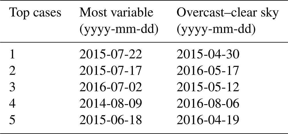
In order to find specific types of case studies for analysis, one can use either the event statistics or daily statistics to query and filter specific conditions. As an example, we use the daily statistics file and Python's Xarray to find case studies of the most variable irradiance throughout the day or specific cases where overcast conditions transition to clear sky (or vice versa), which have the potential for brief periods of strong variability and cloud enhancement. These example are shown in Table 2, and the code is publicly available (Sect. 5).
Table 2Examples of finding case studies using daily statistics. For a custom period (2014–2016), the table shows the top five cases for two example queries. The first is the absolute most variable weather with respect to irradiance. The second query is cases with at least 5 % overcast, variable, and clear sky, sorted by those with the most variability, which is a way to find case studies with overcast to clear-sky transitions.
The 1 Hz GHI, DIF, and DNI observations of the BSRN station at Cabauw are published on Zenodo (https://doi.org/10.5281/zenodo.7093164, Knap and Mol, 2022), Irradiance time series classifications, supplementary data, quality control, event and daily statistics, and satellite data are published as a separate, complementary dataset on Zenodo (https://doi.org/10.5281/zenodo.7462362, Mol et al., 2022). Satellite data for an area around Cabauw are taken from the CLAAS-2 open-access dataset described in Benas et al. (2017) (DOI: https://doi.org/10.5676/EUM_SAF_CM/CLAAS/V002, Finkensieper et al., 2016) and included in the previous dataset for 2014 to 2016. Moreover, the NubiScope data (Wauben et al., 2010), taken from the KNMI Data Platform (https://dataplatform.knmi.nl/dataset/cesar-nubiscope-cldcov-la1-t10-v1-0, KNMI, 2023), for the years 2014 to 2016 are also included. All code to reproduce the classifications from the irradiance observations, event and daily statistics, and figures presented in this paper is archived at https://doi.org/10.5281/zenodo.7851741 (Mol, 2023).
In this paper, we describe a high-resolution, 10-year-long observational dataset of detailed surface solar irradiance that is complemented with meteorological data. Using time series classification algorithms, we derive statistics about sky type and irradiance variability. We provide examples and use cases of this dataset to illustrate its potential, ranging from case study selection and model validation to fundamental insight into drivers of irradiance variability. With all data and processing code publicly available, the user is free to modify our classification algorithm to their liking and validate it against independent observations or to expand upon the large set of statistics already provided. Quicklooks for all available days from February 2011 to December 2020 are provided in order for the user to become familiar with the dataset contents and to get an impression of the many different types of weather conditions at Cabauw. We believe that this dataset is of great use in research into cloud-driven irradiance variability, and it provides a necessary validation reference for models that are starting to resolve the full spectrum of variability.
WBM performed the data analysis, produced the public datasets, and wrote the manuscript. WHK is the BSRN Cabauw station scientist and maintained and produced the original 1 Hz irradiance dataset. CCvH helped shape the manuscript and is the project PI. All authors contributed to the final paper.
The contact author has declared that none of the authors has any competing interests.
Publisher’s note: Copernicus Publications remains neutral with regard to jurisdictional claims in published maps and institutional affiliations.
Wouter B. Mol and Chiel C. van Heerwaarden have received funding from the Dutch Research Council (NWO; grant no. VI.Vidi.192.068).
This paper was edited by Tobias Gerken and reviewed by Tobias Gerken and one anonymous referee.
Benas, N., Finkensieper, S., Stengel, M., van Zadelhoff, G.-J., Hanschmann, T., Hollmann, R., and Meirink, J. F.: The MSG-SEVIRI-based cloud property data record CLAAS-2, Earth Syst. Sci. Data, 9, 415–434, https://doi.org/10.5194/essd-9-415-2017, 2017. a, b
Driemel, A., Augustine, J., Behrens, K., Colle, S., Cox, C., Cuevas-Agulló, E., Denn, F. M., Duprat, T., Fukuda, M., Grobe, H., Haeffelin, M., Hodges, G., Hyett, N., Ijima, O., Kallis, A., Knap, W., Kustov, V., Long, C. N., Longenecker, D., Lupi, A., Maturilli, M., Mimouni, M., Ntsangwane, L., Ogihara, H., Olano, X., Olefs, M., Omori, M., Passamani, L., Pereira, E. B., Schmithüsen, H., Schumacher, S., Sieger, R., Tamlyn, J., Vogt, R., Vuilleumier, L., Xia, X., Ohmura, A., and König-Langlo, G.: Baseline Surface Radiation Network (BSRN): structure and data description (1992–2017), Earth Syst. Sci. Data, 10, 1491–1501, https://doi.org/10.5194/essd-10-1491-2018, 2018. a
Durand, M., Murchie, E. H., Lindfors, A. V., Urban, O., Aphalo, P. J., and Robson, T. M.: Diffuse solar radiation and canopy photosynthesis in a changing environment, Agr. Forest Meteorol., 311, 108684, https://doi.org/10.1016/j.agrformet.2021.108684, 2021. a
Ehrlich, A. and Wendisch, M.: Reconstruction of high-resolution time series from slow-response broadband terrestrial irradiance measurements by deconvolution, Atmos. Meas. Tech., 8, 3671–3684, https://doi.org/10.5194/amt-8-3671-2015, 2015. a
Finkensieper, S., Meirink, J.-F., van Zadelhoff, G.-J., Hanschmann, T., Benas, N., Stengel, M., Fuchs, P., Hollmann, R., and Werscheck, M.: CLAAS-2: CM SAF CLoud property dAtAset using SEVIRI – Edition 2, Satellite Application Facility on Climate Monitoring [data set], https://doi.org/10.5676/EUM_SAF_CM/CLAAS/V002, 2016. a
Gristey, J. J., Feingold, G., Glenn, I. B., Schmidt, K. S., and Chen, H.: Surface Solar Irradiance in Continental Shallow Cumulus Fields: Observations and Large-Eddy Simulation, J. Atmos. Sci., 77, 1065–1080, https://doi.org/10.1175/JAS-D-19-0261.1, 2020. a, b
Gschwind, B., Wald, L., Blanc, P., Lefèvre, M., Schroedter-Homscheidt, M., and Arola, A.: Improving the McClear model estimating the downwelling solar radiation at ground level in cloud-free conditions – McClear-v3, metz, 28, 147–163, https://doi.org/10.1127/metz/2019/0946, 2019. a
Gueymard, C. A.: Cloud and albedo enhancement impacts on solar irradiance using high-frequency measurements from thermopile and photodiode radiometers. Part 1: Impacts on global horizontal irradiance, Sol. Energy, 153, 755–765, https://doi.org/10.1016/j.solener.2017.05.004, 2017. a, b, c, d
Helbig, M., Gerken, T., Beamesderfer, E. R., Baldocchi, D. D., Banerjee, T., Biraud, S. C., Brown, W. O. J., Brunsell, N. A., Burakowski, E. A., Burns, S. P., Butterworth, B. J., Chan, W. S., Davis, K. J., Desai, A. R., Fuentes, J. D., Hollinger, D. Y., Kljun, N., Mauder, M., Novick, K. A., Perkins, J. M., Rahn, D. A., Rey-Sanchez, C., Santanello, J. A., Scott, R. L., Seyednasrollah, B., Stoy, P. C., Sullivan, R. C., de Arellano, J. V.-G., Wharton, S., Yi, C., and Richardson, A. D.: Integrating continuous atmospheric boundary layer and tower-based flux measurements to advance understanding of land-atmosphere interactions, Agr. Forest Meteorol., 307, 108509, https://doi.org/10.1016/j.agrformet.2021.108509, 2021. a
Jakub, F. and Mayer, B.: A three-dimensional parallel radiative transfer model for atmospheric heating rates for use in cloud resolving models – The TenStream solver, J. Quant. Spectrosc. Ra., 163, 63–71, https://doi.org/10.1016/j.jqsrt.2015.05.003, 2015. a
Kipp & Zonen: CH1 Pyrheliometer Instruction Manual, https://www.kippzonen.com/Download/42/CH-1-Pyrheliometer-Manual-English (last access: 26 July 2022), 2001. a
Kipp & Zonen: CM22 precision pyranometer instruction manual, https://www.kippzonen.com/Download/55/CM-22-Pyranometer-Manual (last access: 26 July 2022), 2004. a
Kivalov, S. N. and Fitzjarrald, D. R.: Quantifying and Modelling the Effect of Cloud Shadows on the Surface Irradiance at Tropical and Midlatitude Forests, Bound.-Lay. Meteorol., 166, 165–198, https://doi.org/10.1007/s10546-017-0301-y, 2018. a, b
Knap, W.: Basic and other measurements of radiation at station Cabauw (2005-02 et seq), PANGAEA [data set], https://doi.org/10.1594/PANGAEA.940531, 2022. a, b
Knap, W. H. and Mol, W. B.: High resolution solar irradiance variability climatology dataset part 1: direct, diffuse, and global irradiance, Zenodo [data set], https://doi.org/10.5281/zenodo.7093164, 2022. a, b, c
KNMI: Cloud cover retrieved from infrared measurements at 10 minute intervals at CESAR observatory, KNMI [data set], https://dataplatform.knmi.nl/dataset/cesar-nubiscope-cldcov-la1-t10-v1-0, last access: 16 May 2023. a
Liang, X.: Emerging Power Quality Challenges Due to Integration of Renewable Energy Sources, IEEE T. Ind. Appl., 53, 855–866, https://doi.org/10.1109/TIA.2016.2626253, 2017. a
Lohmann, G. M.: Irradiance Variability Quantification and Small-Scale Averaging in Space and Time: A Short Review, Atmosphere, 9, 264, https://doi.org/10.3390/atmos9070264, 2018. a
Lohmann, G. M., Monahan, A. H., and Heinemann, D.: Local short-term variability in solar irradiance, Atmos. Chem. Phys., 16, 6365–6379, https://doi.org/10.5194/acp-16-6365-2016, 2016. a
Mercado, L. M., Bellouin, N., Sitch, S., Boucher, O., Huntingford, C., Wild, M., and Cox, P. M.: Impact of changes in diffuse radiation on the global land carbon sink, Nature, 458, 1014–1017, https://doi.org/10.1038/nature07949, 2009. a
Mol, W.: Code for 1 Hz solar irradiance processing and variability analyses, Zenodo [code], https://doi.org/10.5281/zenodo.7851741, 2023. a
Mol, W. and Heusinkveld, B.: Radiometer grid at Falkenberg and surroundings, downwelling shortwave radiation, FESSTVaL campaign, Universität Hamburg [data set], https://doi.org/10.25592/uhhfdm.10273, 2022. a
Mol, W. B., Knap, W. H., and van Heerwaarden, C. C.: High resolution solar irradiance variability climatology dataset part 2: classifications, supplementary data, and statistics, Zenodo [data set], https://doi.org/10.5281/zenodo.7462362, 2022. a, b, c, d, e, f
Mol, W. B., van Stratum, B. J. H., Knap, W. H., and van Heerwaarden, C. C.: Reconciling Observations of Solar Irradiance Variability With Cloud Size Distributions, 128, e2022JD037894, https://doi.org/10.1029/2022JD037894, 2023. a, b, c, d, e
NOAA: Climate Algorithm Theoretical Basis Document, Tech. Rep., https://ncei.noaa.gov/pub/data/sds/cdr/CDRs/Cloud_Properties-ISCCP/AlgorithmDescription_01B-29.pdf (last access: 16 May 2023), 2022. a
Pearcy, R. W. and Way, D. A.: Two decades of sunfleck research: looking back to move forward, Tree Physiol., 32, 1059–1061, https://doi.org/10.1093/treephys/tps084, 2012. a
Tabar, M. R. R., Anvari, M., Lohmann, G., Heinemann, D., Wächter, M., Milan, P., Lorenz, E., and Peinke, J.: Kolmogorov spectrum of renewable wind and solar power fluctuations, Eur. Phys. J. Spec. Top., 223, 2637–2644, https://doi.org/10.1140/epjst/e2014-02217-8, 2014. a, b, c
Tijhuis, M., van Stratum, B., van Heerwaarden, C., and Veerman, M.: An Efficient Parameterization for Surface Shortwave 3D Radiative Effects in Large-Eddy Simulations of Shallow Cumulus Clouds, ESS Open Archive [preprint], https://doi.org/10.1002/essoar.10511758.2, 2022. a
van Heerwaarden, C. C., Mol, W. B., Veerman, M. A., Benedict, I., Heusinkveld, B. G., Knap, W. H., Kazadzis, S., Kouremeti, N., and Fiedler, S.: Record high solar irradiance in Western Europe during first COVID-19 lockdown largely due to unusual weather, Communications Earth & Environment, 2, 37, https://doi.org/10.1038/s43247-021-00110-0, 2021. a
van Stratum, B., van Heerwaarden, C. C., and Vilà-Guerau de Arellano, J.: The Benefits and Challenges of Downscaling a Global Reanalysis with Doubly-Periodic Large-Eddy Simulations, ESS Open Archive [preprint], https://doi.org/10.22541/essoar.168167362.25141062/v1, 2023. a
Veerman, M. A., van Stratum, B. J. H., and van Heerwaarden, C. C.: A case study of cumulus convection over land in cloud-resolving simulations with a coupled ray tracer, Geophys. Res. Lett., 49, e2022GL100808, https://doi.org/10.1029/2022GL100808, 2022. a, b, c
Wauben, W., Bosveld, F., and Baltink, H. K.: Laboratory and Field Evaluation of the NubiScope Conference: WMO Technical Conference on Meteorological and Environmental Instruments and Methods of Observation, TECO-2010, WMO, Helsinki, https://library.wmo.int/pmb_ged/wmo-td_1546_en/1_7_Waubenetal_Netherlands.pdf (last access: 16 May 2023), 2010. a, b, c
WMO: Chapter 8 – Measurement of sunshine duration, https://library.wmo.int/index.php?lvl=notice_display&id=19664 (last access: 6 July 2022), 2014. a
Yang, D., Wang, W., Gueymard, C. A., Hong, T., Kleissl, J., Huang, J., Perez, M. J., Perez, R., Bright, J. M., Xia, X., van der Meer, D., and Peters, I. M.: A review of solar forecasting, its dependence on atmospheric sciences and implications for grid integration: Towards carbon neutrality, Renew. Sust. Energ. Rev., 161, 112348, https://doi.org/10.1016/j.rser.2022.112348, 2022. a
Yordanov, G. H.: A study of extreme overirradiance events for solar energy applications using NASA’s I3RC Monte Carlo radiative transfer model, Sol. Energy, 122, 954–965, https://doi.org/10.1016/j.solener.2015.10.014, 2015. a
Yordanov, G. H., Saetre, T. O., and Midtgård, O.: 100-millisecond Resolution for Accurate Overirradiance Measurements, IEEE J. Photovolt., 3, 1354–1360, https://doi.org/10.1109/JPHOTOV.2013.2264621, 2013. a
Yordanov, G. H., Saetre, T. O., and Midtgård, O.-M.: Extreme overirradiance events in Norway: 1.6 suns measured close to 60∘ N, Sol. Energy, 115, 68–73, https://doi.org/10.1016/j.solener.2015.02.020, 2015. a