An iterative labeling method for annotating marine life imagery

1 Introduction

Technologies for imaging the deep seafloor have evolved significantly over the last three decades (Durden et al., 2016). These technologies have enabled the study and monitoring of the spatiotemporal changes of marine life in the vast ocean space. They should ultimately enable us to conduct more efficient fishery independent surveys, yielding improved stock assessments and ecosystem-based management (Francis et al., 2007). Manned submersibles, Remotely Operated Vehicles (ROVs), Autonomous Underwater Vehicles (AUVs) (Singh et al., 2004b), towed vehicles (Taylor et al., 2008), and bottom-mounted and midwater cameras (Amin et al., 2017) have all contributed to an explosion of data in terms of our ability to obtain high-resolution, true-color (Kaeli et al., 2011) camera imagery underwater.

The reality, however, is that extracting actionable information from our large underwater image datasets remains a challenging task. The ability to process the data is not proportional to the rate at which the data is acquired, as traditional methods were resource-intensive in terms of manpower, time, and cost. Efforts are underway to analyze the imagery with various levels of automation using tools from machine learning for a variety of fisheries and habitat monitoring applications, including coral reefs (Singh et al., 2004a; Gleason et al., 2007; Purser et al., 2009; Chen et al., 2021), starfish (Clement et al., 2005; Smith and Dunbabin, 2007), scallops (Dawkins et al., 2017), and commercially important groundfish (Tolimieri et al., 2008).

In parallel, there have been significant developments in deep learning (Krizhevsky et al., 2012; Simonyan and Zisserman, 2014), which further propelled these efforts by truly leveraging the availability of large amounts of data. Multiple works have explored the use of standard deep convolutional neural networks for image segmentation and classification (Ramani and Patrick, 1992; Anantharajah et al., 2014; Boom et al., 2014; Cutter et al., 2015; Fisher et al., 2016; Marburg and Bigham, 2016; Sung et al., 2017; Kaveti and Singh, 2018; Wang et al., 2021). Reinforcement learning has been used to enhance underwater imagery to improve the performance of object detection networks, (Wang et al., 2023; yu Wang et al., 2023). These works have helped marine biologists analyze underwater imagery far more efficiently.

1.1 Generation of labeled underwater datasets

The remarkable success of deep learning techniques is primarily due to the availability of large labeled datasets. A number of public underwater image databases, such as FathomNet (Katija et al., 2021), EcoTaxa (Blue-Cloud, 2019), DeepFish (Saleh et al., 2020), WildFish++ (Zhuang et al., 2021), and BIIGLE 2.0 (Langenkämper et al., 2017), have come into existence in recent years. These works provide a platform and tools for annotating, uploading, and downloading annotated images, and sometimes also training or testing machine learning models. Generating labeled datasets by manually going through vast amounts of video and image streams is a time-consuming task. Several efforts have been initiated toward machine learning-assisted automation for annotating underwater datasets. CoralNet 1.0 (Chen et al., 2021) is a data repository that also deploys a feature extractor network pre-trained on a large collection of data to generate annotations of coral reefs automatically. (Zurowietz et al., 2018) propose a multi-stage method where an auto encoder network generates training proposals that are filtered by human observers and used to train a segmentation network, the results of which are further reviewed manually.

However, these annotation approaches require human experts with marine biology knowledge, which makes it difficult to generalize and scale to huge volumes of data. In fact, there are a large number of underwater image datasets available with no efficient means to label them. One such example is shown in Figure 1. The absence of well-labeled data is still a primary factor limiting the widespread use of machine learning techniques for marine science research.

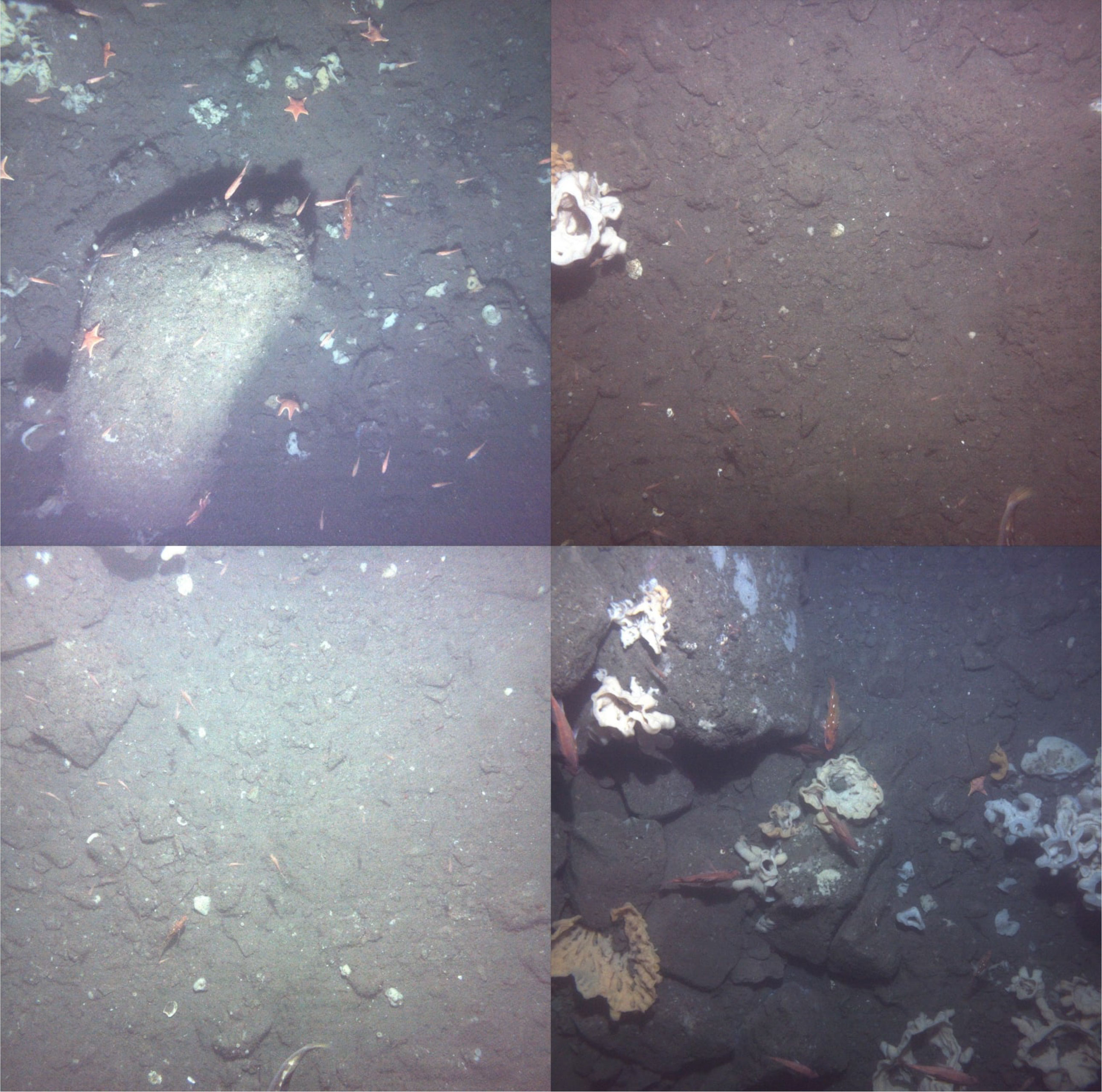
Figure 1 Underwater image samples from one of the datasets with no annotations. There are very large marine life related image datasets that are freely available but are not annotated. These would require significant efforts from experts in the field to label.

One simple solution is to utilize crowdsourcing platforms involving non-expert human users, such as Mechanical Turk (Crowston, 2012) and Zooniverse (Simpson et al., 2014) Crowdsourcing platforms are fairly inexpensive and highly efficient for the rapid generation of annotated datasets. But the results for specialized imagery, such as that associated with marine biology, are often mixed and unreliable. Our own experience has shown that some workers annotate images with randomly placed labels, which requires a prohibitive amount of time and effort spent approving or rejecting these results.

1.2 Performance enhancement on crowdsourcing platforms

Many human-machine collaboration methods have been proposed to improve the efficiency of human in-the-loop annotation. Branson et al. (2010) presents an interactive, hybrid human-computer method for image classification. Deng et al. (2014) focuses on multi-label annotation, which finds the correlation between objects in the real world to reduce the human computation time required for checking their existence in the image. Russakovsky et al. (2015) asks human annotators to answer a series of questions to check and update the predicted bounding boxes, while Wah et al. (2011) queries the user with binary questions to locate the part of the object. Vijayanarasimhan and Grauman (2008) incrementally updates the classifier by requesting multi-level annotations, ranging from full segmentation to a present/absent flag on the image. Kaufmann et al. (2011) and Litman et al. (2015) adapt different models from motivation theory and have studied the effect of extrinsic and intrinsic motivation on worker performance.

Some recent research has shown that when non-experts are trained and clearly instructed on the annotation protocol, they can produce accurate results (Cox et al., 2012; Matabos et al., 2017; Langenkämper et al., 2019), thus demonstrating the potential for combining citizen science with machine learning. Kaveti and Akbar (2020) designed an enhanced MTurk interface and added a guided practice test to achieve higher annotation accuracy. Bhattacharjee and Agrawal (2021) simplified complex tasks on MTurk by combining batches, dummy variables, and worker qualifications. Our work is most similar to LSUN (Yu et al., 2015), in that they hid ground truth labels in the task to verify worker performance and allowed multiple workers to label the same image for quality control.

Thus, we propose a human-in-the-loop annotation methodology that can label very large datasets automatically by combining machine learning with Mechanical Turk crowdsourcing. We utilize a unique iterative process with auto-approval that allows us to check the quality of the workers algorithmically, precisely, efficiently, and without any human intervention. We can also use the same techniques for converting historical expert annotations, as shown in Figure 2A, to quickly create labeled data sets for machine learning that are critically required for fisheries and ecosystem-based management applications.

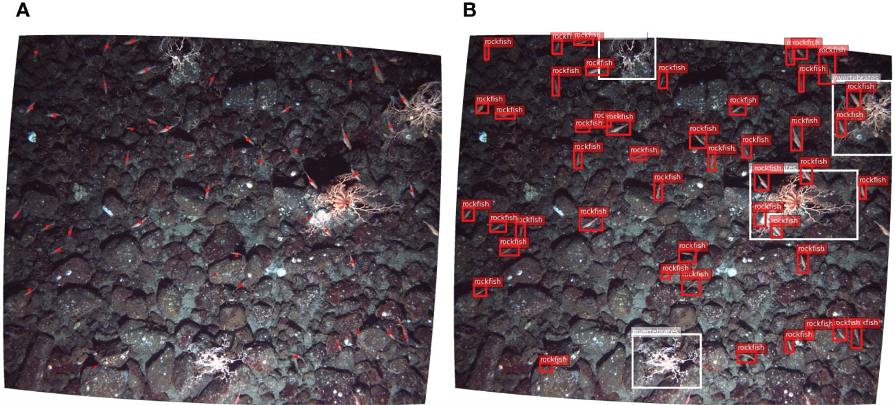
Figure 2 NOAA annotation ground truth (A) Underwater images annotated by NOAA marine biologists, with dot annotations on each object. (B) Extended dot annotations to bounding box labels with MTurk workers.

In contrast to LSUN (Yu et al., 2015), we only label once per object during the iterative labeling process if the category is not controversial. We define our task as working with individual objects in an image, as opposed to considering all the objects in an entire image. Additionally, we remove qualification tests and add tutorials to lower the barriers for workers to enter our tasks. In this way, we can provide the simplest form of the task to Mechanical Turk workers.

2 The iterative labeling process

The overview of our method for the iterated labeling process for underwater images is illustrated in Figure 3. The process begins by building an initial deep learning model for making bounding box predictions on a small subset of underwater images. These predictions are then published to a crowdsourcing platform with a well-designed assistive interface for validation. An auto-approval method filters out bad labels from the crowdsourcing platform. The filtered labels are added to the dataset and used for further training to generate new predictions. Therefore, we start with a small set of annotations and increase the number of annotations with each loop until all objects in all images have been labeled. Figure 4 shows an example of the predict-update loop for a single image.

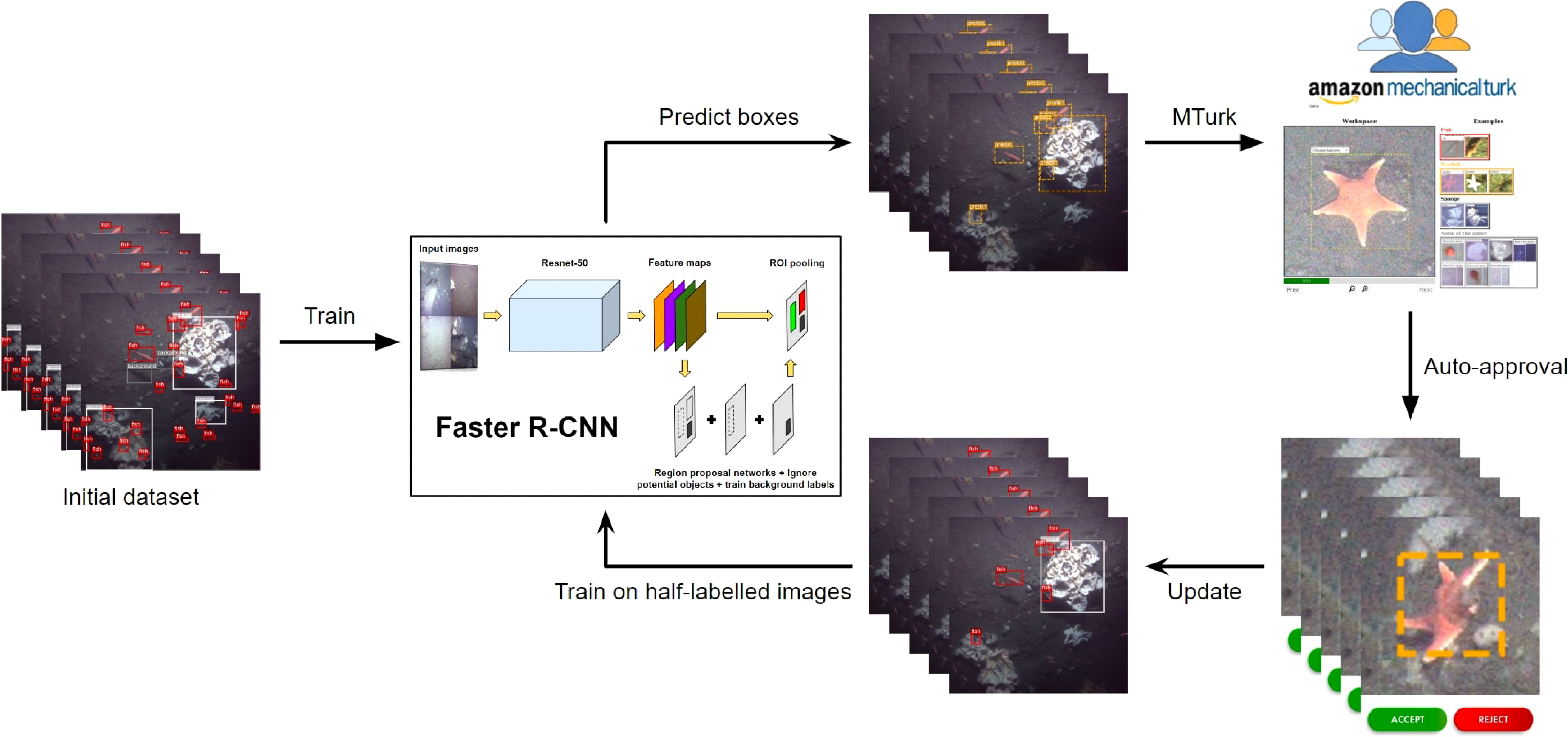
Figure 3 The complete iterative labeling process: We begin by training the initial dataset with Faster R-CNN (Ren et al., 2015) in order to obtain an initial model. Next, we use this initial model to predict objects in a new image set, and publish the prediction boxes to MTurk for correction. Auto-approval filters the labeling results. Then, we update the labels and train on half-labeled images to obtain a new model and prediction set for the next loop. Finally, we converge to a completely labeled dataset in 3-6 iterations.

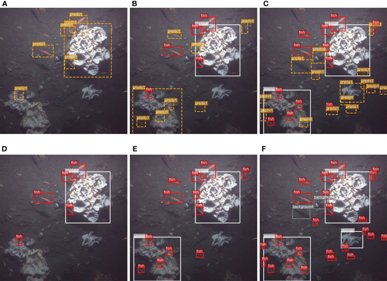
Figure 4 An example of the iterative labeling process. The orange dashed boxes represent the predictions of each loop. These prediction boxes are published to MTurk for correction. The updated labels, based on the MTurk results, are then used for the next iteration (A) Loop 1 predict, (B) Loop 2 predict, (C) Loop 3 predict, (D) Loop 1 update, (E) Loop 2 update, (F) Loop 3 update.

2.1 The initial model

We start with a small seed dataset labeled by marine biologists. This serves as our initial dataset, which we use to train our deep learning object detection model. The seed dataset should consist of different forms of the object that we are about to label. In our case, this data is not large enough to completely train a high accuracy model, but it is sufficient to make reasonable predictions to feed into the first iteration of our process.

As the iterative labeling process does not have real-time constraints, we chose Faster R-CNN (Ren et al., 2015) as the object detection network in combination with ResNet-50 (He et al., 2015) as the backbone network. Feature Pyramid Networks (Lin et al., 2016) were applied for multi-scale object detection. We built the network based on Detectron2 (Wu et al., 2019). We trained the object detection network on 2 RTX 2080 GPUs with a batch size of 2 for 60 epochs. Since the batch size is very small, group normalization (Wu and He, 2018) was used instead of batch normalization. Typically, we use less than 100 images for the initial dataset, and the initial data only takes a few hours to label.

After training the initial model, we utilize it to predict the learned object categories on new unlabeled image data. However, as there is no ground truth available for this data, we cannot be certain if these predictions are true positives. To address this issue, we enlist workers from Mechanical Turk to classify and correct the predictions.

2.2 Assistive annotation interface design

In this section, we describe the design and development of the user interface on MTurk used to facilitate the human-in-the-loop learning process. One of the key aspects of the interface is presenting the user with a convenient way to determine the accuracy of the deep learning model’s predictions, and to annotate them if they are correct. These correct object detections are then used as ground truth labels to continue training the deep learning model. The fundamental idea is that through a series of predict (using our algorithm), correct and update (with Mechanical Turk workers), and train (using our algorithm) loops, we will end up with a superior model.

The most common interface design for labeling object instances in images on MTurk requires workers to detect all objects in the image and draw bounding boxes for each object before moving on to the next image. This process can be cumbersome when there are a lot ($>$ 30) of instances per image to label and is especially challenging when the dataset consists of unique, specialized categories of objects. This can also affect the worker’s motivation to perform the task (Kaveti and Akbar, 2020). We have made a few novel design choices to construct our MTurk annotation interface, as described below. Figure 5 shows a snapshot of our assistive annotation interface.

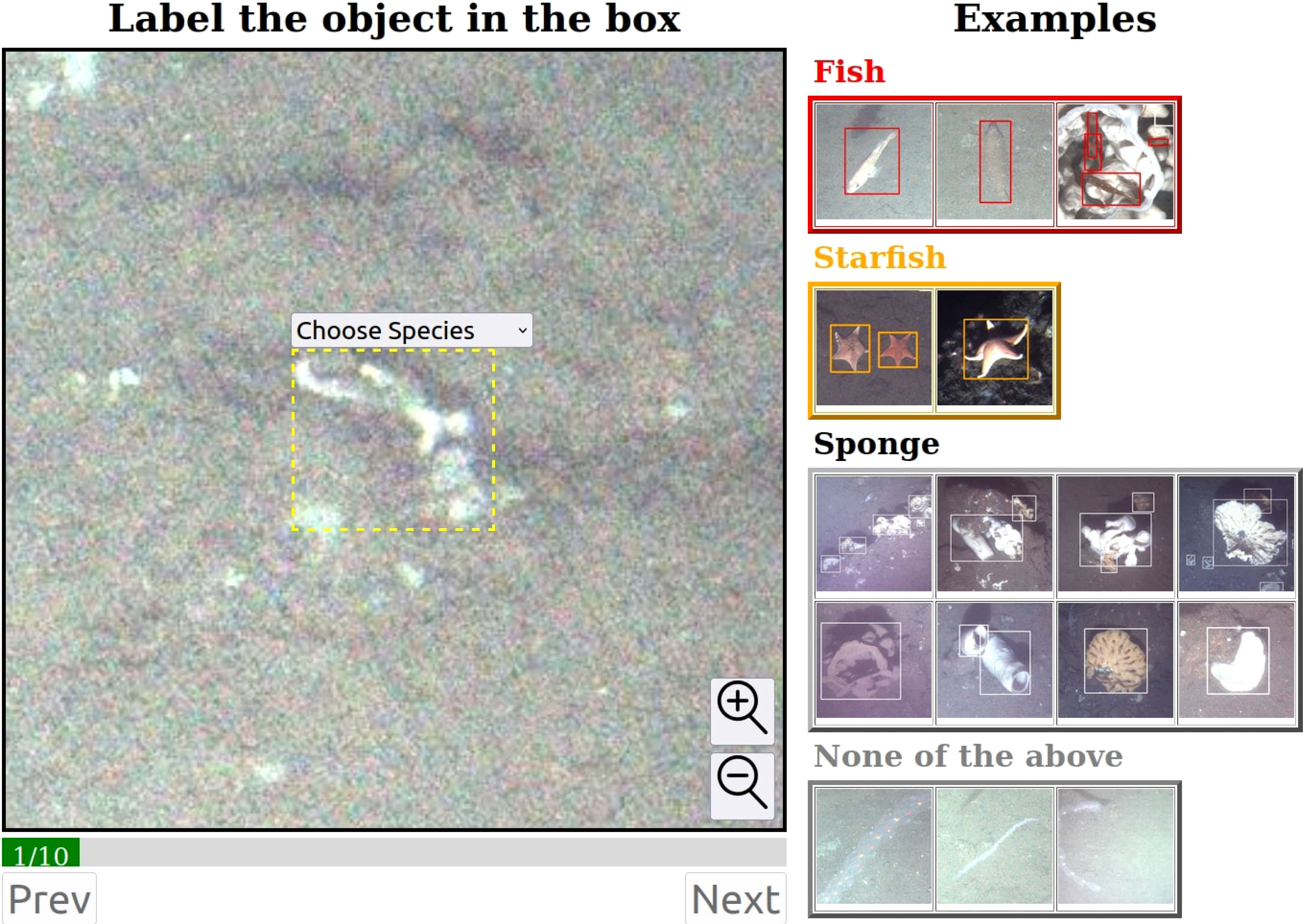
Figure 5 The Assistive Interface is designed to help MTurk workers by providing them with a tool to focus on a specific object. By simply identifying the species and fitting the bounding box, the labels’ reliability is significantly improved. The ground truth is hidden at the last task to implement auto-approval.

2.2.1 Tutorial/examples of annotations

One of the challenges of underwater datasets is that they contain unique and uncommon objects. Moreover, the workers on MTurk come from diverse backgrounds with variability in experience and expertise. To address this issue, we have dedicated a small portion of the interface to showcase a set of labeling examples for the various marine species encountered in the dataset. This helps to familiarize workers with the dataset and improve the quality of their labeling.

2.2.2 Labeling cues

Instead of asking workers to find all possible instances of categories in a raw image, we provide several labeling cues to make it easy for them. We show the predictions made by the deep learning model as a dashed bounding box. The workers are then asked to adjust it to tightly fit the object and choose the species from a dropdown menu. These features help correct localization and classification losses during supervision. Sometimes, the background in images can be mistakenly predicted as a species. To address this issue, we added a “None of the above” option to the species dropdown menu, which corresponds to the background.

2.2.3 UI controls

The images in our underwater dataset can contain 40-50 instances of relevant objects per image. Sometimes, these instances can be really small and occluded by other objects due to overlap, as shown in Figure 4. Therefore, we choose to zoom in and display each bounding box prediction individually, rather than showing all of the boxes at the same time. This allows workers to focus on a single object at a time, which is beneficial for labeling tiny objects and also improves user performance when adjusting the bounding boxes.

2.3 The auto-approval process

The biggest drawback of the MTurk platform is with respect to the quality control of workers. Although MTurk allows one to select workers based on certain criteria or through a test, requesters often end up spending a lot of time and resources reviewing annotation results. This negates the purpose of wanting to create a fully automated human-in-the-loop annotation process. Therefore, we have developed an auto-approval mechanism to assess how well workers are performing and to accept or reject annotations without any intervention.

The auto-approval is accomplished by randomly hiding ground truth tests in the labeling tasks. Each MTurk task consists of nine labeling tasks and one ground truth test task. The ground truth labels are obtained from a manual labeling, which comes from the initial and validation datasets. We compare the worker’s labeled bounding box to the ground truth bounding box, and compute the intersection over union (IOU) of the two bounding boxes. We accept the worker’s annotations only if the IoU score is higher than the threshold of 0.75. LSUN (Yu et al., 2015) proposes a similar method, using hidden ground truth data to validate the MTurk labeling results. However, they use the entire image as a labeling task, while we use every single object.

2.3.1 Double checking identifications

The incorrect classification of objects can lead to incorrect training. Therefore, even if a sub-task has passed the hidden ground truth test, we still need to double-check the class that is chosen. If the selected class is different from the predicted class, we add the sub-task to the republish list. Meanwhile, we change the class of the predicted box to the one selected by the current worker. This means that the class of the object is determined only if two consecutive workers choose the same category. Otherwise, the prediction box would be repeatedly republished under this mechanism. If an object is actually a background, it would be republished at least twice to fully determine that it is the background.

To get a sense of the efficiency and cost of the process, we examined one representative batch of tasks that was given to MTurk workers. In this batch, there were 4,583 tasks. Each task required 9 labels and 1 ground truth test, and cost three cents, which works out to a cent for three labels. On average, each task took 3 minutes and 5 seconds to complete, and our tasks are easy to complete. For the entire batch, it took about 6 hours to finish all the tasks. Out of the 4,583 tasks in this particular batch, 3,413 tasks were auto-approved as passed, while 1,170 were rejected.

2.4 Training on half-labeled images

In the first iteration, where the prediction is based on the initial model, not all object instances in the images will be discovered, and the accuracy of the predictions cannot be guaranteed. This is because the initial model is trained only on a small seed dataset, which is insufficient to fully train the model. These predictions are sent to MTurk for correction. The new bounding boxes are then used to supervise the training of our deep learning model, which in turn makes new and more accurate predictions. However, since the object labels of the images are incomplete, some issues arise in the training process. Therefore, we make modifications to the training phase, including feeding appropriate training data and loss functions to suit our iterative labeling process. The detailed changes to the loss function can be found in 2.4.4.

2.4.1 Modifications to Faster R-CNN to avoid negative mining of potential objects

During the training of an object detection model, if an object is not labeled in the images, it will be implicitly treated as a background class. This is especially true for algorithms such as SSD (Liu et al., 2015) and Faster R-CNN (Ren et al., 2015), which use negative hard sampling to train the background class. In SSD, the top N highest confidence predictions that do not match any ground truth are selected and trained as negative samples. Meanwhile, Faster R-CNN randomly selects a certain percentage of prediction boxes without matching ground truths as negative samples. However, this can cause serious issues with our training because if half of the objects in the image are not labeled, it will prevent the trained model from converging.

The solution to this issue is to identify unlabeled potential objects and avoid training them as negative samples. When the prediction confidence score of an anchor exceeds a specific threshold and there are no ground truth objects that match that prediction, it implies that the model thinks there may be a potential object at that spot. Therefore, this object should be ignored in the training process to be discovered later, as shown in Figure 6. In the Region Proposal Network (RPN) of Faster R-CNN, we mark all the prior anchors whose confidence score exceeds 0.5 without a ground truth label as “ignored”. We exclude them from being selected as negative samples for loss calculations and also prevent them from being selected to enter the next stage of the process, which is the region of interest (ROI) layer.

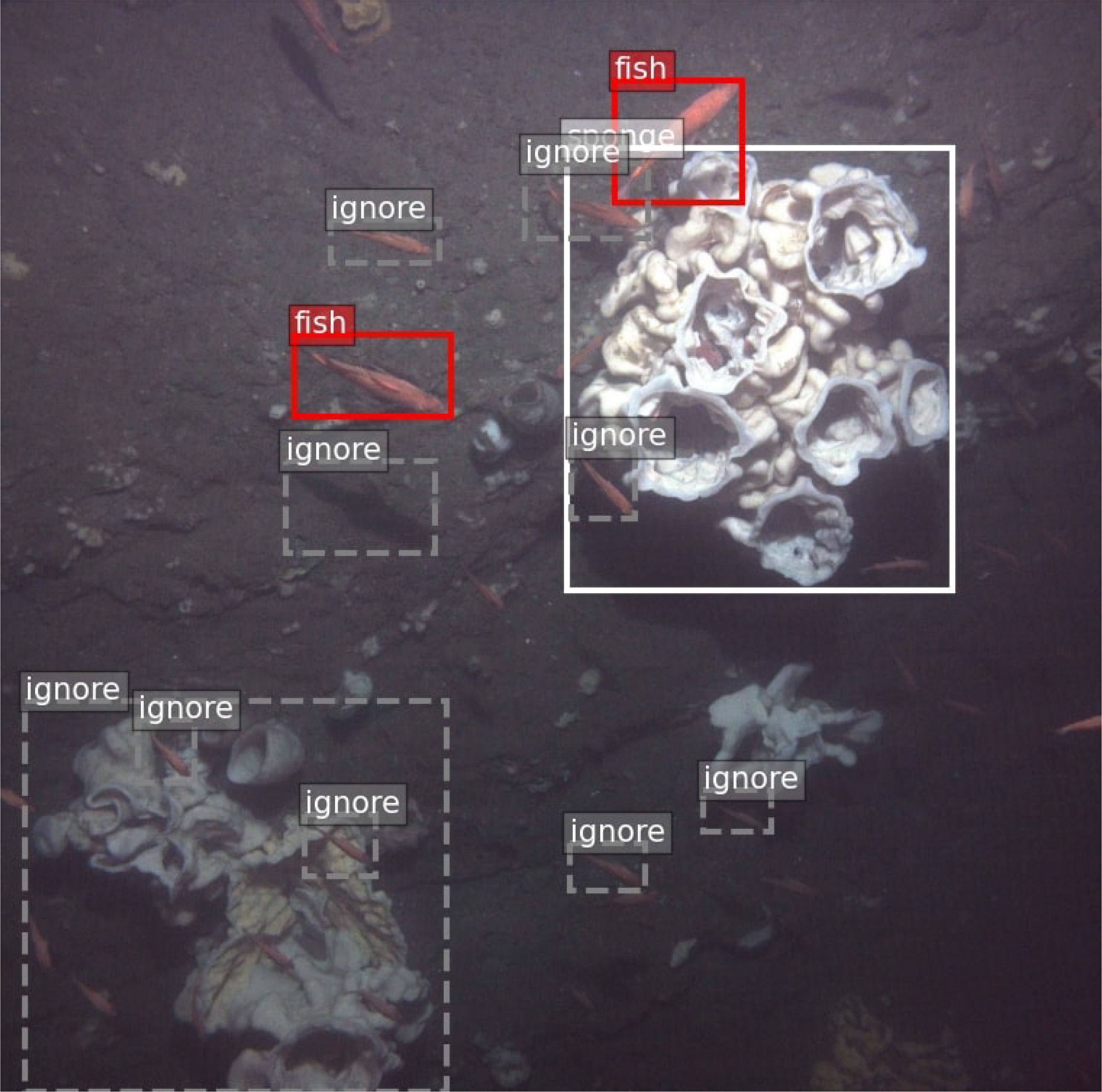
Figure 6 Ignoring potential objects: The dashed bounding boxes represent potential objects with a significant classification score that have not yet been verified and labeled. These unlabeled objects may be wrongly classified as negative samples during training iterations, leading to an incorrect model. To avoid this, we detect potential objects using a classification score threshold and exclude them from the training process.

2.4.2 Training background labels

In the previous section, we described how to avoid training potential true positive predictions as a background class. In this section, we discuss how to correctly train the false positive (background) class. During the iterative labeling process, some predictions are false positives and are corrected as “background” by the MTurk workers. These background labels can be used in the training process.

In the Region Proposal Network (RPN), instead of randomly selecting negative samples, the boxes that are updated as the “background” class from the MTurk auto-approval process should be trained. When the number of negative samples is significant, the probability of being trained as a potential object is very low. This is valuable because it increases the precision of our object detection model and avoids ignoring potential objects. We do not calculate the localization loss of background labels as they are negative samples, and their use ends with the RPN. Training background labels properly can reduce false positives, in other words, increasing the precision of the model.

2.4.3 Data augmentation

We also perform data augmentation to generate more training samples. All the images are put through the following transformations: a flip of the image horizontally and vertically, adjustments to brightness by scaling the intensity randomly between 0.8 and1.2, and a random scaling factor corresponding to 0.8 to 1.0 of the image size.

2.4.4 Loss function

Taking into account the above mentioned changes to the training phase, the loss function can be divided into four components:

•The classification loss, ${\displaystyle {\sum }_i{L}_{cls}(p_i,p_i^{*})}$, where the predicted labels have object class ground truths associated with them. ground truth bounding boxes are obtained from MTurk after auto-approval. $N$: RPN mini-batch size

•The classification loss ${\displaystyle {\sum }_j{L}_{cls}(p_j,p_j^{*})}$, where a background class ground truth box is associated with the predicted label. This ground truth is also obtained from MTurk after the auto-approved label is selected as back-ground.

•The classification loss ${\displaystyle {\sum }_k{L}_{cls}(p_k,p_k^{*})]}$, where the predicted box does not have any ground truth box associated with it but the prediction score with respect to an object class is less than 0.5. In this case we consider this as a negative sample.

•The regression loss $\lambda \frac{1}{N}{\displaystyle {\sum }_i{L}_{reg}(t_i,t_i^{*})}$ which is computed for the predicted labels which have object class ground truth boxes associated with them.

Putting all the components together the loss function can be written as

The classification loss is:

The localization loss is:

where $i$ is the index of an anchor in a mini-batch, whose ground truth is an object. $j$ is the index of an anchor, whose ground truth is a labeled background. $k$ is the index of an anchor, which has no ground truth and $p_k$ is lower than the ignore threshold. $p_{i,j,k}$ is the predicted probability of being an object. $p_{i,j,k}^{*}$ is the ground truth probability where 1 indicates that it is foreground. 0 means background. Here $p_i^{*}=1,p_{j,k}^{*}=0$. $t_i$ is a vector representing the 4 parameterized coordinates of the prediction bounding box. $t_i^{*}$ is the ground truth box associated with a positive anchor. $\lambda$ is the balancing parameter of object and localization loss.

3 Results and discussions

3.1 Labeling a ground truth dataset

We have a large dataset with dot annotations provided by NOAA marine biologists (Figure 2A). These annotations were made before the advent of machine learning techniques and are unsuitable for machine learning applications due to the absence of bounding boxes around the objects. However, this dataset is ideal for setting up, testing, and validating our efforts. We could then transfer to other datasets with completely unlabeled data, as we discuss in the next section.

We publish these dot labels to MTurk workers using our assistive interface (see Figure 5). The workers can extend the dot annotations to create tight and accurate bounding boxes with the help of the instructions. An example of the extended bounding boxes is shown in Figure 2B. We consider them as ground truth labels to validate the iterative labeling process.

We divided our dataset into two parts, using 51 images as the initial dataset and 632 images as our validation dataset (Table 1). We then applied our iterative labeling process to the remaining 9822 images.

Table 1 NOAA dataset with ground truth validation.

Table 1 shows the iterative labeling results. We ran six iterations to annotate the dataset. The initial dataset is very small (534 labels, 51 images), and the trained model is relatively poor (0.6 mAP). In the first loop, most of the rockfish were labeled, as these are easy for the deep learning model to identify. As the images were half-labeled, we chose to ignore the threshold of 0.5 to prevent training the model on rockfish with prediction scores over 0.5. As the loops iterated, the mAP and recall rate increased, enabling the trained model to detect more rockfish. In the final loop, the mAP and recall rate stopped growing, indicating that the model was unable to detect any more rockfish. We used this as a stopping mechanism for our iterations.

There are a reasonable number of rockfish that are very hard to detect. Typically, these are small and have low contrast (see Figure 7A). To help our algorithm cope with these issues, we crop the large-size image (2448 x 2050) into nine sub-images, each measuring 896 x 896. During prediction, we crop the image in the same way to maintain scale consistency. We also adjust the contrast of the images to perform data augmentation. In the end, about 82% of the rockfish are labeled correctly with very few false positives.

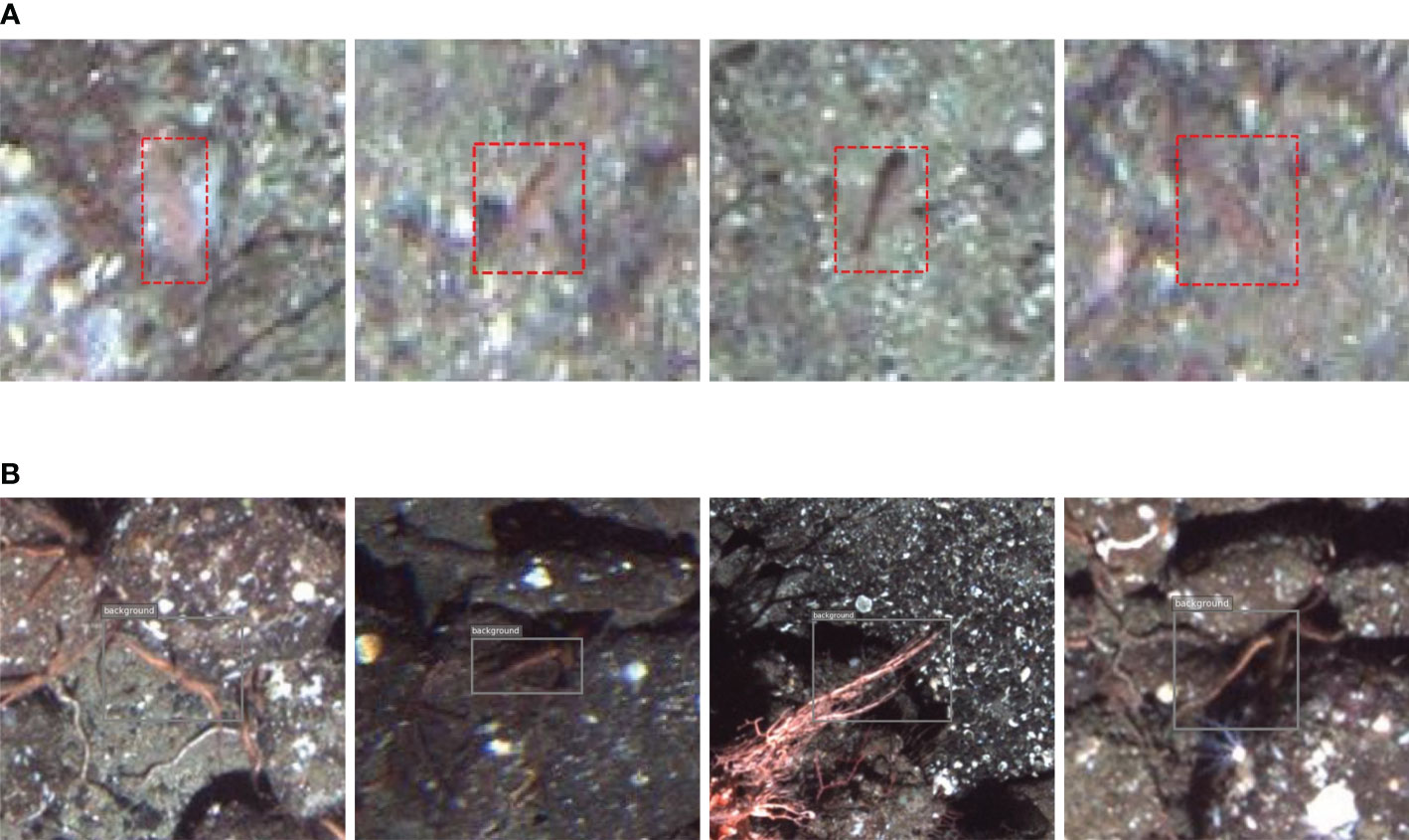
Figure 7 (A) Examples of rockfish that our algorithm missed (false negatives). Usually, these specimens are very small and have low contrast. (B) Examples of background labels (false positives) for rockfish. Usually, the false positives are either parts of starfish or other invertebrates. Training background labels properly can increase the precision of the model.

Along with rockfish labels, we also generate background labels to identify false positives. These false positives typically include starfish or invertebrates that resemble fish (see Figure 7B).

We should also point out that the NOAA dataset has been annotated to a greater level of taxonomic resolution, including coral, flatfish, groundfish, etc. The classification of the data to such levels uses very detailed markings and is an interesting and open problem beyond the scope of this work.

3.2 Labeling a dataset with sponges

Our second illustrative dataset, the Pacstorm dataset, contains three categories of marine organisms: fish, starfish, and sponge. In this case, we used 98 images as the initial dataset and 302 as our validation data. We ran the iterative labeling process on the remaining 3,568 images to generate labels (see Table 2).

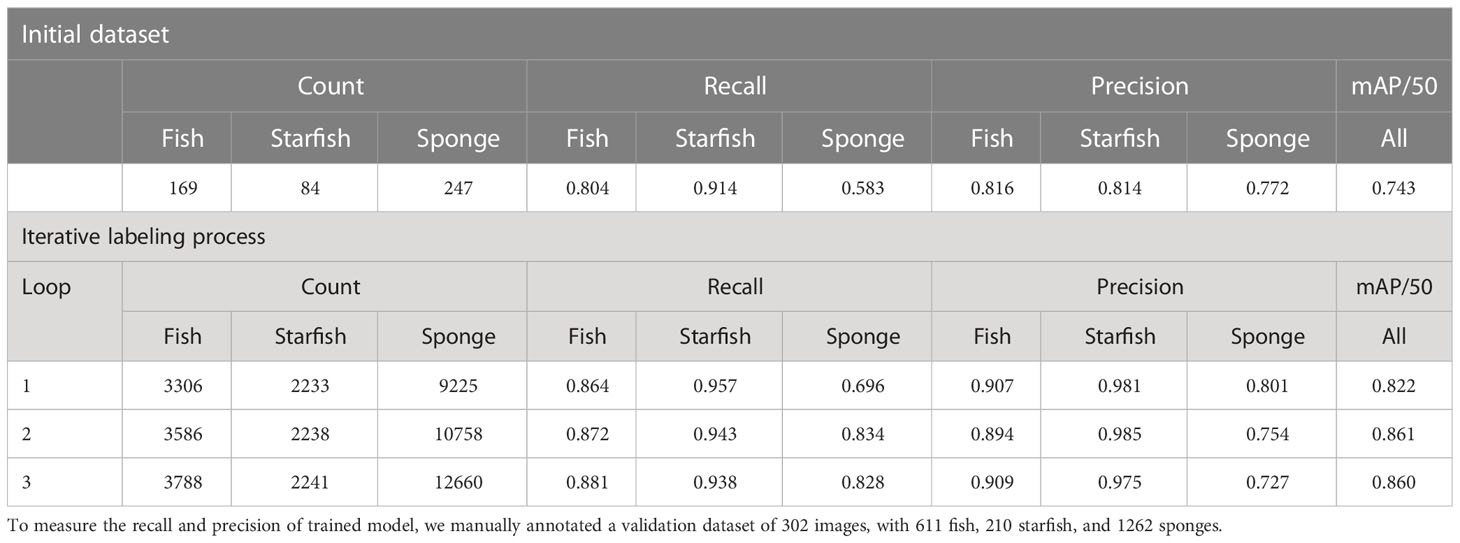
Table 2 The Pacstorm dataset which consists of fish, starfish and sponges.

In this dataset, fish and starfish are easy to identify and label, but sponges are far more challenging. The reasons for this are manifold. The sponges have many different forms (as shown in Figure 8A). Some sponges have a hole on top, while others do not. Some sponges look like white rocks, and others look like white dots. Sponges also have different colors; while most of them are white, some are brown, and dead sponges are black. The trickiest problem is that the sponges can group together (as shown in Figure 8B), making it hard to decide whether to annotate all of them with one label or annotate them separately. Some sponges are covered in mud, with only a small part of them exposed (as shown in Figure 8C). The variety of cases not only confuses the deep learning model but also the MTurk workers. When annotating the initial and validation dataset, these problems make it difficult to maintain consistency in labeling patterns for sponges.

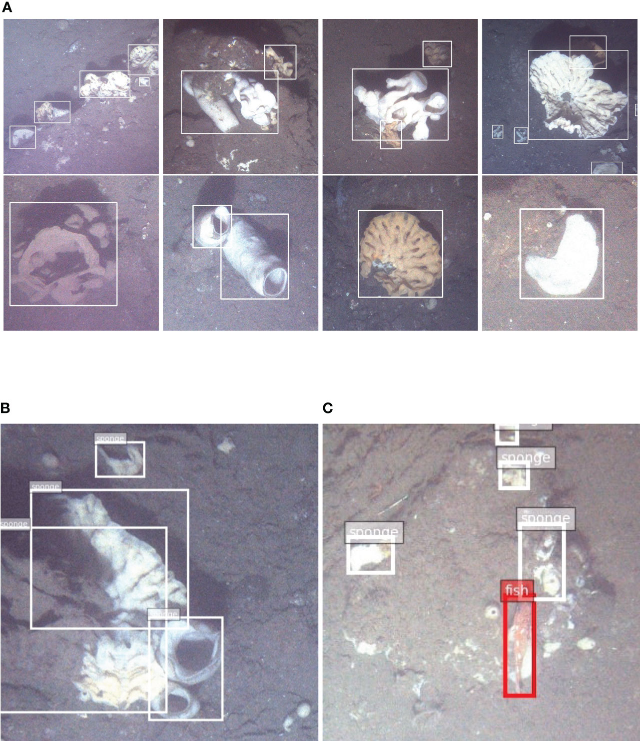
Figure 8 (A)Examples of different forms of sponges. Some sponges have a hole on top, while others do not. Some sponges look like white rocks, and others look like white dots. Sponges also come in different colors. While most of them are white, some are brown, and dead sponges are black. We presented these examples to the MTurk workers to help them identify the sponges. (B) Sometimes sponges are grouped together, which make it very hard to label them individually. (C) Some sponges are covered in mud, with only small part of them exposed. This make us hard to determine the labeling standard.

To overcome the problem of different shapes and colors, we presented a large number of sponge examples alongside the assistive annotation interface for worker training. By grouping the sponges together, we can avoid predicting small sponges within a large labeled sponge group.

In the final count, we labeled 12,660 sponges, 3,588 fish, and 2,241 starfish in 3,568 images (Table 2). The recall rate roughly shows the coverage of the iterative labeling process. In this case, about 90% of the fish and sponges were detected and labeled, and over 83% of the sponges were well-labeled. Additionally, we trained an efficient model with an mAP of about 0.86, corresponding to these labels.

4 Conclusion

In this paper, we present a method for rapidly labeling large underwater datasets. We demonstrate that this method is robust, effective, and efficient for annotating a large number of images containing difficult classes. We began with a small initial dataset and utilized an iterative labeling process that gradually generates bounding box annotations. Our method results in a dataset with high coverage of rockfish, starfish, and sponge annotations after only a few iterations.

We first obtained the NOAA dataset, which only had dot annotations. We utilized MTurk workers to extend the dots to bounding boxes with the help of an assistive labeling interface. Then, we used these annotations as ground truth to validate our approach. We applied the iterative labeling process to 9,822 images and labeled 82% of the rockfish.

Next, we applied the same process to the empty Pacstorm dataset that we wanted to label, which included the challenging sponge class. After three iterations, we were able to label 90% of the fish and starfish and 83% of the sponges.

Both datasets are freely available for other researchers to use via our website. A direct link to the website is available in the Data Availability Statement below. We hope that this data, as well as the algorithm, can serve as a benchmark for validating various machine learning methodologies for marine biology related applications.

Author's note

Author AP was employed under contract at NOAA by Lynker Technologies at the time of researching this study.

Data availability statement

The datasets presented in this study can be found in online repositories. The names of the repository/repositories and accession number(s) can be found below: https://fieldroboticslab.ece.northeastern.edu/resources/.

Author contributions

PK contributed to the main conceptual ideas and designed the study. ZZ implemented the proposed method and performed experimental analysis on the datasets. HS, MC, and AP supervised the project and gave valuable feedback on the results. AP, EF, and MC provided the underwater fisheries datasets used in this study. EF helped verify the annotations generated by the proposed method by comparing them with manual annotations. ZZ took the lead in writing the manuscript and PK wrote a few sections in the manuscript. All authors contributed to the article and approved the submitted version.

Conflict of interest

The authors declare that the research was conducted in the absence of any commercial or financial relationships that could be construed as a potential conflict of interest.

Publisher’s note

All claims expressed in this article are solely those of the authors and do not necessarily represent those of their affiliated organizations, or those of the publisher, the editors and the reviewers. Any product that may be evaluated in this article, or claim that may be made by its manufacturer, is not guaranteed or endorsed by the publisher.

References

Amin R., Richards B. L., Misa W. F. X. E., Taylor J. C., Miller D. R., Rollo A. K., et al. (2017). The modular optical underwater survey system (MOUSS) for in situ sampling of fish assemblages. Sensors (Basel Switzerland) 17, 1–8. doi: 10.3390/s17102309
Anantharajah K., Ge Z., McCool C., Denman S., Fookes C., Corke P., et al. (2014). “Local inter-session variability modelling for object classification,” in IEEE Winter Conference on Applications of Computer Vision. 309–316.
Bhattacharjee A., Agrawal M. (2021). Process design to use amazon mturk for cognitively complex tasks. IT Prof. 23, 56–61. doi: 10.1109/MITP.2020.2983395
Blue-Cloud (2019). Ecotaxa. Available at: https://blue-cloud.org/data-infrastructures/ecotaxa
Boom B., He J., Palazzo S., Huang P. X., Beyan C., Chou H.-M., et al. (2014). A research tool for long-term and continuous analysis of fish assemblage in coral-reefs using underwater camera footage. Ecol. Inf. 23, 83–97. doi: 10.1016/j.ecoinf.2013.10.006
Branson S., Wah C., Schroff F., Babenko B., Welinder P., Perona P., et al. (2010). Visual recognition with humans in the loop. in. Eur. Conf. Comput. Vision. doi: 10.1007/978-3-642-15561-1_32
Chen Q., Beijbom O., Chan S., Bouwmeester J., Kriegman D. J. (2021). “A new deep learning engine for coralnet,” in 2021 IEEE/CVF International Conference on Computer Vision Workshops (ICCVW). 3686–3695.
Clement R., Dunbabin M. D., Wyeth G. (2005). Towards robust image detection of crown-of-thorns starfish for autonomous population monitoring. Environ. Sci.
Cox T. E., Philippoff J., Baumgartner E. S., Smith C. M. (2012). Expert variability provides perspective on the strengths and weaknesses of citizen-driven intertidal monitoring program. Ecol. Appl. Publ. Ecol. Soc. America 22 (4), 1201–1212. doi: 10.1890/11-1614.1
Crowston K. (2012). “Amazon Mechanical turk: a research tool for organizations and information systems scholars,” in Shaping the future of ICT research (Berlin, Heidelberg: Springer Berlin Heidelberg), 210–221.
Cutter G. R., Stierhoff K., Zeng J. (2015). “Automated detection of rockfish in unconstrained underwater videos using haar cascades and a new image dataset: labeled fishes in the wild,” in 2015 IEEE Winter Applications and Computer Vision Workshops. 57–62.
Dawkins M., Sherrill L., Fieldhouse K., Hoogs A., Richards B. L., Zhang D. C., et al. (2017). “An open-source platform for underwater image and video analytics,” in 2017 IEEE Winter Conference on Applications of Computer Vision (WACV). 898–906.
Deng J., Russakovsky O., Krause J., Bernstein M. S., Berg A. C., Fei-Fei L. (2014). “Scalable multi-label annotation,” in Proceedings of the SIGCHI Conference on Human Factors in Computing Systems (New York, NY, USA: Association for Computing Machinery), 3099–3102.
Durden J. M., Schoening T., Althaus F., Friedman A., Garcia R. V., Glover A. G., et al. (2016). Perspectives in visual imaging for marine biology and ecology: from acquisition to understanding. Oceanogr. Mar. Biol. 54, 1–72. doi: 10.1201/9781315368597-2
Fisher R. B., Shao K.-T., Chen-Burger Y.-H. J. (2016). “Overview of the fish4knowledge project,” in Fish4Knowledge.
Francis R., Hixon M. A., Clarke M., Murawski S., Ralston S. (2007). Ten commandments for ecosystem-based fisheries scientists. Fisheries 32, 217–233. doi: 10.1577/1548-8446(2007)32[217:TCFBFS]2.0.CO;2
Gleason A. C. R., Reid R. P., Voss K. J. (2007). Automated classification of underwater multispectral imagery for coral reef monitoring. OCEANS 2007, 1–8. doi: 10.1109/OCEANS.2007.4449394
He K., Zhang X., Ren S., Sun J. (2015). “Deep residual learning for image recognition,” in 2016 IEEE Conference on Computer Vision and Pattern Recognition (CVPR). 770–778.
Kaeli J. W., Singh H., Murphy C., Kunz C. (2011). “Improving color correction for underwater image surveys,” in OCEANS’11 MTS/IEEE KONA. 1–6.
Katija K., Orenstein E. C., Schlining B., Lundsten L., Barnard K., Sainz G., et al. (2021). Fathomnet: a global image database for enabling artificial intelligence in the ocean. Sci. Rep. 12, 15914. doi: 10.1038/s41598-022-19939-2
Kaufmann N., Schulze T., Veit D. J. (2011). “More than fun and money. worker motivation in crowdsourcing - a study on mechanical turk,” in Americas conference on information systems.
Kaveti P., Akbar M. N. (2020). “Role of intrinsic motivation in user interface design to enhance worker performance in amazon mturk,” in Proceedings of the 13th ACM International Conference on PErvasive Technologies Related to Assistive Environments.
Kaveti P., Singh H. (2018). “Towards automated fish detection using convolutional neural networks,” in 2018 OCEANS - MTS/IEEE Kobe Techno-Oceans (OTO). 1–6.
Krizhevsky A., Sutskever I., Hinton G. E. (2012). Imagenet classification with deep convolutional neural networks. Commun. ACM 60, 84–90. doi: 10.1145/3065386
Langenkämper D., Simon-Lledó E., Hosking B., Jones D. O. B., Nattkemper T. W. (2019). On the impact of citizen science-derived data quality on deep learning based classification in marine images. PLoS One 14. doi: 10.1371/journal.pone.0218086
Langenkämper D., Zurowietz M., Schoening T., Nattkemper T. W. (2017). Biigle 2.0 - browsing and annotating large marine image collections. Front. Mar. Sci. 4. doi: 10.3389/fmars.2017.00083
Lin T.-Y., Dollár P., Girshick R. B., He K., Hariharan B., Belongie S. J. (2016). “Feature pyramid networks for object detection,” in 2017 IEEE Conference on Computer Vision and Pattern Recognition (CVPR). 936–944.
Litman L., Robinson J., Rosenzweig C. (2015). The relationship between motivation, monetary compensation, and data quality among us- and india-based workers on mechanical turk. Behav. Res. Methods 47, 519–528. doi: 10.3758/s13428-014-0483-x
Liu W., Anguelov D., Erhan D., Szegedy C., Reed S. E., Fu C.-Y., et al. (2015). “Ssd: single shot multibox detector,” in European Conference on Computer Vision (Cham: Springer International Publishing), 21–37.
Marburg A., Bigham K. (2016). “Deep learning for benthic fauna identification,” in OCEANS 2016 MTS/IEEE Monterey. 1–5.
Matabos M., Hoeberechts M., Doya C., Aguzzi J., Nephin J., Reimchen T. E., et al. (2017). Expert, crowd, students or algorithm: who holds the key to deep-sea imagery ‘big data’ processing? Methods Ecol. Evol. 8, 996–1004. doi: 10.1111/2041-210X.12746
Purser A., Bergmann M., Lundälv T., Ontrup J., Nattkemper T. W. (2009). Use of machine-learning algorithms for the automated detection of cold-water coral habitats: a pilot study. Mar. Ecol. Prog. Ser. 397, 241–251. doi: 10.3354/meps08154
Ramani N., Patrick P. H. (1992). “Fish detection and identification using neural networks-some laboratory results,” in IEEE Journal of Oceanic Engineering, Vol. 17. 364–368.
Ren S., He K., Girshick R. B., Sun J. (2015). “Faster r-cnn: towards real-time object detection with region proposal networks,” in IEEE Transactions on Pattern Analysis and Machine Intelligence, Vol. 39. 1137–1149.
Russakovsky O., Li L.-J., Fei-Fei L. (2015). “Best of both worlds: human-machine collaboration for object annotation,” in 2015 IEEE Conference on Computer Vision and Pattern Recognition (CVPR). 2121–2131.
Saleh A., Laradji I. H., Konovalov D. A., Bradley M., Vázquez D., Sheaves M. (2020). A realistic fish-habitat dataset to evaluate algorithms for underwater visual analysis. Sci. Rep. 10, 14671. doi: 10.1038/s41598-020-71639-x
Simonyan K., Zisserman A. (2014). “Very deep convolutional networks for large-scale image recognition,” in CoRR abs/1409. 1556.
Simpson R. J., Page K. R., Roure D. C. D. (2014). “Zooniverse: observing the world’s largest citizen science platform,” in Proceedings of the 23rd International Conference on World Wide Web.
Singh H., Armstrong R. A., Gilbes F., Eustice R. M., Roman C., Pizarro O., et al. (2004a). Imaging coral i: imaging coral habitats with the seabed auv. Subsurface Sens. Technol. Appl. 5, 25–42. doi: 10.1023/B:SSTA.0000018445.25977.f3
Singh H., Can A., Eustice R. M., Lerner S., McPhee N. M., Roman C. (2004b). “Seabed auv offers new platform for high-resolution imaging,” in Eos, Transactions Am. Geophys. Union Vol. 85. 289–296.
Smith D. V., Dunbabin M. D. (2007). “Automated counting of the northern pacific sea star in the derwent using shape recognition,” in 9th Biennial Conference of the Australian Pattern Recognition Society on Digital Image Computing Techniques and Applications (DICTA 2007). 500–507.
Sung M., Yu S.-C., Girdhar Y. A. (2017). “Vision based real-time fish detection using convolutional neural network,” in OCEANS 2017, Aberdeen. 1–6.
Taylor R., Vine N., York A., Lerner S., Hart D., Howland J. C., et al. (2008). “Evolution of a benthic imaging system from a towed camera to an automated habitat characterization system,” in OCEANS 2008. 1–7.
Tolimieri N., Clarke M., Singh H., Goldfinger C. (2008). Evaluating the seabed auv for monitoring groundfish in untrawlable habitat. Mar. Habitat Mapping Technol. Alska doi: 10.4027/mhmta.2008.09
Vijayanarasimhan S., Grauman K. (2008). “Multi-level active prediction of useful image annotations for recognition,” in NIPS.
Wah C., Branson S., Perona P., Belongie S. J. (2011). “Multiclass recognition and part localization with humans in the loop,” in 2011 International Conference on Computer Vision. 2524–2531.
Wang H., Sun S., Bai X., Wang J., Ren P. (2023). A reinforcement learning paradigm of configuring visual enhancement for object detection in underwater scenes. IEEE J. Oceanic Eng. 48, 443–461. doi: 10.1109/JOE.2022.3226202
Wang H., Sun S., Wu X., Li L., Zhang H., Li M., et al. (2021). “A yolov5 baseline for underwater object detection,” in OCEANS 2021, San Diego – Porto. 1–4.
Wu Y., He K. (2018). “Group normalization,” in International Journal of Computer Vision, Vol. 128. 742–755.
Wu Y., Kirillov A., Massa F., Lo W.-Y., Girshick R. (2019) Detectron2. Available at: https://github.com/facebookresearch/detectron2.
Yu F., Zhang Y., Song S., Seff A., Xiao J. (2015). Lsun: construction of a large-scale image dataset using deep learning with humans in the loop. ArXiv. bs/1506.03365. doi: 10.48550/arXiv.1506.03365
yu Wang H., Sun S., Ren P. (2023). “Meta underwater camera: a smart protocol for underwater image enhancement,” in ISPRS Journal of Photogrammetry and Remote Sensing. 462–481. Available at: https://www.sciencedirect.com/science/article/pii/S0924271622003227.
Zhuang P., Wang Y., Qiao Y. (2021). “Wildfish++: a comprehensive fish benchmark for multimedia research,” in IEEE Transactions on Multimedia, Vol. 23. 3603–3617.
Keywords: iterative labeling, active learning, Faster R-CNN, NOAA, Amazon MTurk, auto-approval, background label
Citation: Zhang Z, Kaveti P, Singh H, Powell A, Fruh E and Clarke ME (2023) An iterative labeling method for annotating marine life imagery. Front. Mar. Sci. 10:1094190. doi: 10.3389/fmars.2023.1094190
Received: 09 November 2022; Accepted: 03 May 2023;
Published: 26 May 2023.
Edited by:
Mark C. Benfield, Louisiana State University, United StatesReviewed by:
Shinnosuke Nakayama, Stanford University, United StatesPeng Ren, China University of Petroleum (East China), China
Copyright © 2023 Zhang, Kaveti, Singh, Powell, Fruh and Clarke. This is an open-access article distributed under the terms of the Creative Commons Attribution License (CC BY). The use, distribution or reproduction in other forums is permitted, provided the original author(s) and the copyright owner(s) are credited and that the original publication in this journal is cited, in accordance with accepted academic practice. No use, distribution or reproduction is permitted which does not comply with these terms.
*Correspondence: Zhiyong Zhang, zhang.zhiyo@northeastern.edu