Testing indicators for trend assessment of range and habitat of low-density cetacean species in the Mediterranean Sea

1 Introduction

The conservation of cetacean species is extremely challenging due to the large extent of their range and their highly dynamic migratory nature. The European Environmental Agency (EEA) Report (No 10/2020) states that “marine mammals (including cetaceans) are among the species with the highest proportion of unknown assessments (over 78%)”. Data deficiency is mainly due to the fact that most cetacean species inhabit remote offshore areas which are more difficult to monitor due to logistical reasons linked to both the organisation of surveys and political barriers as coordinating effort in areas overcoming socio-political borders requires a functional international cooperation. Moreover, the high costs generally required for carrying out regular large-scale surveys limit the ability to gather sufficient information, especially on rare species.

1.1 Low-density cetacean species conservation status in the Mediterranean Sea

In the Mediterranean Sea, Risso’s dolphin (Grampus griseus, Gg), long-finned pilot whale (Globicephala melas, Gm), and Cuvier’ beaked whale (Ziphius cavirostris, Zc), are considered low-density elusive species. Their assessment status under the IUCN Red list of threatened species recently changed from ‘Data Deficient’ to, respectively, ‘Endangered’ (Gg, Lanfredi et al., 2021), and ‘Vulnerable’ (Gm, Gauffier and Verborgh, 2021; Zc, Cañadas and Notarbartolo di Sciara, 2018). A distinct subpopulation of long-finned pilot whales, limited to the Strait of Gibraltar area, and listed as ‘Critically Endangered’, was also identified during the last assessment (Verborgh and Gauffier, 2021). The three species are listed in Annex IV of the EU Habitats Directive (HD, Directive 92/43/EEC) as species requiring a special protection regime across their natural range, both within and outside the Natura 2000 sites, to enable their Favourable Conservation Status (FCS) to be maintained or, where appropriate, restored, in their natural range. The core areas of their habitat must be identified, designated as Sites of Community Importance, included in the Natura 2000 network, and managed in accordance with their ecological needs. Moreover, Member States must regularly report to the EU on their conservation status. Cetaceans are also a target species of Descriptor 1 (Biodiversity) of the Marine Strategy Framework Directive (MSFD, Directive 2008/56/EC), which aims at achieving a Good Environmental Status (GES) of EU marine waters by establishing a common approach and objectives for the prevention, protection and conservation of the marine environment. Thus, information about the preferred habitats of cetacean species and the early detection of potential changes in their distribution is essential to identify needed conservation measures.

1.2 Overview of approaches for assessing range and habitat trends

Despite the fact that the HD focuses on the conservation status of the species (i.e., the effects), and the MSFD on eliminating the causes (i.e., the threats) through mitigation measures that will restore the GES (Palialexis et al., 2019), the HD and MSFD have strong synergies. Under the MSFD, Member States are required to establish threshold values for each species through regional or sub-regional cooperation and, for species covered by the HD, these values shall be consistent with the Favourable Reference Values (FRV) established under the HD. Both HD and MSFD directives require reporting every six years equivalent parameters/criteria for the assessment of the species conservation status such as ‘Range’ (i.e., HD ‘The natural range of the species is neither being reduced nor is likely to be reduced for the foreseeable future’; MSFD D1C4 ‘the species distributional range and, where relevant, the pattern, is in line with prevailing physiographic, geographic and climatic conditions’) and ‘Habitat’ (i.e., HD ‘There is, and will probably continue to be, a sufficiently large habitat to maintain its populations on a long-term basis’; MSFD D1C5 ‘The habitat for the species has the necessary extent and condition to support the different stages in the life history of the species’). Similarly, the EO1 assessment within the Barcelona Regional Sea Convention (UNEP-MAP, EO1) is based on the Common Indicators (CI) 3 (‘Species distributional range’) and 1 (‘Habitat distributional range’). The IUCN Guidelines for the assessment of the conservation status of threatened species also foresee the assessment based on the criteria A2c (‘A decline in Area Of Occupancy-AOO, Extent Of Occurrence-EOO and/or habitat quality’) and B (‘Geographic range’). Specifically, the AOO is defined as ‘the area contained within the shortest continuous imaginary boundary that can be drawn to encompass all the known, inferred or projected sites of present occurrence of a taxon, excluding cases of vagrancy’ (IUCN, 2001), where ‘Projected sites’ are considered as the sites spatially predicted on the basis of habitat maps or models (area of potential habitat, also called Extent of Suitable Habitat, ESH). A suspected decline in the AOO could consequently be estimated based on the reduction of suitable habitat. In addition, also the Reporting Guidelines of the Habitats Directive (2017) suggest to evaluate the FRV as the AOO, or as the potential range in relation to available suitable habitat (‘Ecological potential’, the potential extent of range considering physical and ecological conditions).

Within such legal requirements, Species Distribution Modelling (SDM) is a promising approach to support the assessment of cetacean species. Indeed, as long as the amount/quality of input data is reasonably adequate, SDM can be used to support regulatory decision-making for conservation, i.e., by informing on spatial prioritisation through the identification of biodiversity hotspots, important areas for vulnerable species, or valuable habitats, overcoming the problems related to coarse or incomplete knowledge (Franklin, 2010; Maiorano et al., 2019). Time series of comparable data with sufficient statistical power, coupled with standardised SDM analyses, can help identify changes from a reference period. A significant reduction in the extent or a shift of species geographical distribution can then be related to environmental variability, habitat conditions or changes in population size, or to the effect of anthropogenic pressures. Moreover, the comparison of the suitable habitat predicted through SDM with the distributional range observed indicate potential suitable areas that are not used by the species.

However, relevant indicators or threshold values for assessing species range and habitat have not yet been developed (Palialexis et al., 2019), and some recommendations were only recently provided through an international scientific cooperation to define indicators, assessment methods, and data requirements for the assessment of marine turtles under the MSFD (Girard et al., 2022). Moreover, despite an increasing research effort, a limited number of studies attempted so far to infer temporal changes in cetacean distributional range or habitat use, and the ‘trend’ criterion for these parameters/criteria is still considered ‘unknown’ for almost all cetacean species in the Mediterranean Sea (last HD report 2013-2018), likely due to the lack of comparable data and standard methodological approaches.

1.3 Aim of the study

The Fixed Line Transect monitoring Network (FLT Med Net) has been operating in the Mediterranean basin since 2007 collecting cetacean data along fixed trans-border transects regularly surveyed throughout the years. Using the dataset gathered across twelve years, this study aims to improve the knowledge on three low-density cetacean species of the Mediterranean basin Risso’s dolphin (Grampus griseus, Gg), long-finned pilot whale (Globicephala melas, Gm), and Cuvier’s beaked whale (Ziphius cavirostris, Zc), and evaluate potential approaches to support legislative requirements. In particular, using the dataset collected during the third HD six-years reporting cycle (2008-2012) as baseline, the study aims to assess potential changes in the range and habitat of the three species over the subsequent periods (short-term trend) testing four potential indicators: 1) Observed Distributional Range, ODR: changes in the extent of ODR detected within the area covered by monitoring effort; 2) Ecological Potential Range, EPR: change in the extent of Ecological Potential Range predicted by means of SDM; 3) Range Pattern: percentage of overlap, and shifts of ODR and EPR between the two time periods; 4) ODR vs EPR: changes in the proportion of observed distributional range vs the ecological potential range between the two periods. Overall, the study aims to test and evaluate such methodological approaches and indicators to contribute to the species assessment under the requirements of the main European nature legislative framework.

2 Material and methods

2.1 Study area

Cetacean monitoring was carried out from passenger ferries travelling along 11 trans-border transects, covering the Mediterranean Sea within the latitudes 43.6° N - 35.8° S and longitudes -5.5° E - 20.8° E, and connecting Italy, France, Spain, Greece, Tunisia and Morocco. These transects are included in the Fixed Line Transect Mediterranean Network (FLT Med Net, Arcangeli et al., 2019), and are representative of a large proportion of the Western-Mediterranean, the Adriatic Subregions, and two portion eastern and western of Ionian Sea in the Ionian-Central Mediterranean Subregion. Transects considered for the baseline period (2008-2012) covered the effort area shown in gridded grey in Figure 1. In the second period (2013-2019) monitoring was also extended to the area in light grey along the east Spanish coasts and Gibraltar Strait on Western Mediterranean, and in the Adriatic-eastern Ionian Sea.

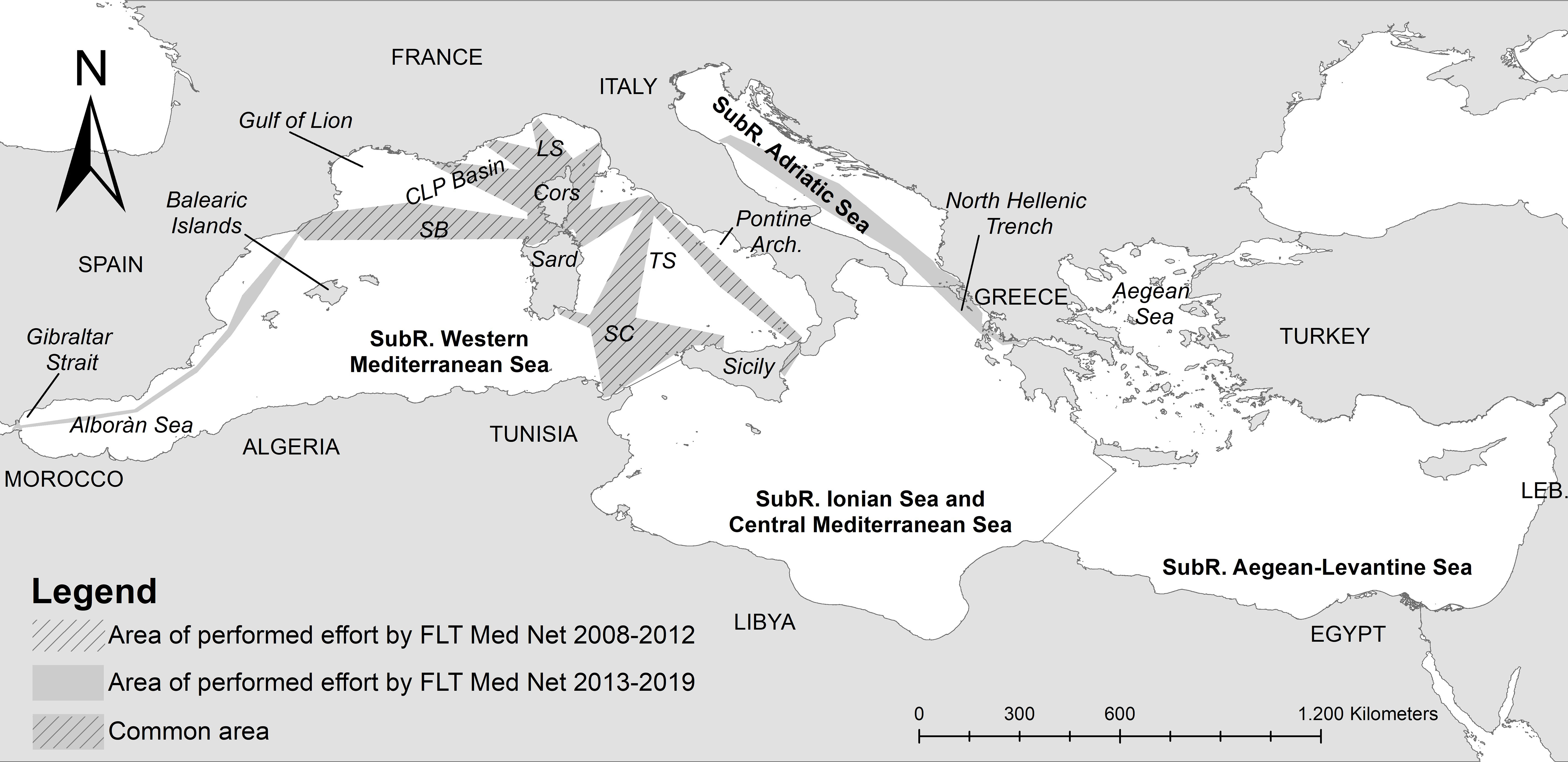
Figure 1 Study Area with the survey effort performed by the FLT Med Net during 2008-2012 (I baseline period, gridded grey only) and 2013-2019 (II period, plain grey). The four Mediterranean MSFD Subregions are shown in the figure: Western-Mediterranean (WMED), central-Mediterranean (Central MED), Adriatic, Aegean-Levantine Sea (downloaded from the European Environment Agency www.eea.europa.eu). LS, Ligurian Sea; CLP Basin, Corso-Ligurian-Provençal Basin; SB, Sardinian-Balearc Basin; TS, Tyrrhenian Sea; SC, Sardinian Channel.

2.2 Data collection

The monitoring activity was performed on a seasonal basis with at least three surveys per season along each sampling transect. Seasons were defined as winter (January to March), spring (April to June), summer (July to September) and autumn (October to December). Data on cetacean species were systematically collected following a standard protocol applied from large vessels (ISPRA, 2015) (FLT Net data, Supplementary Table 1). Ferries provided an observation point at 20−29 m above sea level and travelled at a mean speed in the range of 19−25 knots. Two experienced observers were positioned on the two sides of the command deck scanning both sides of the ship within an angle of 130° ahead in order to avoid re-counting the animals; observations were performed by naked eye and binoculars; binoculars and cameras were used to correctly identify the species and the number of animals. A dedicated GPS was used for automatically recording the survey track at the finest resolution, marking the beginning/ending points and the locations of cetacean sightings. Monitoring was carried out during daylight hours only in optimum weather conditions (≤3 on the Beaufort scale).

2.3 Data analysis

All the analyses performed for this study considered the sighting as the statistical unit, regardless of the number of animals within the sighted group. However, the mean group size was also examined to assess differences between the two periods. Data were analysed considering the different Mediterranean Subregions of the MSFD (https://www.eea.europa.eu/): Western Mediterranean (WMED), Ionian Sea and Central Mediterranean (Central MED), Adriatic, Aegean-Levantine Sea (Figure 1). As data were homogeneously collected within the same set of conditions, detection probabilities were assumed the same across all surveys and between the two survey periods.

2.3.1 Observed distributional range, ODR

As suggested by the HD Guidelines (DG ENV, 2017), the Kernel Density Estimator (KDE) was used to spatially generalize the distribution of the species occurrence and identify the extent and the core areas of species within the region covered by effort. After an initial testing, the KDE analysis was set with a resolution cell of 500 m and search radius of 50,000 m. The 95% isopleth was used to define the extent of ODR, calculated in km².

After calculating the area covered by the effort for each time-period (EffortArea), the proportion of species ODR inside the effort area was calculated per each Subregion and time-period. Then, the ODRs of the two periods were displayed and overlapped, and the temporal trend in the ODR extent was estimated as: Δ distribution = [(ODR/EffortArea_{(2nd period)} – ODR/EffortArea_{(1st period)}) x 100]. Following the OSPAR indicators for seals (Palialexis et al., 2019), threshold values were defined as: if index > 10% = increase, if index < -10% = decrease, otherwise = no change.

2.3.2 Ecological potential range, EPR

The changes in the EPR between the two periods were assessed based on projected sites of species occurrence using spatially predicted sites based on the habitat map models (also called Extent of Suitable Habitat) (IUCN Guidelines, 2001; IUCN, 2022). The following criteria were applied: i) use of adequate spatial resolution for the species knowing their range in the Mediterranean Sea, key variables, and appropriate model validation; ii) validation of suitable maps with independent datasets not used to build models; iii) estimate of the proportion of suitable habitat likely occupied by the species (within the area of effort).

Maximum Entropy (MaxEnt version 3.3.3, http://www.cs.princeton.edu/~schapire/maxent/) was applied to model the relationships between environmental predictors and the occurrence records and to build the Suitable Habitat Maps for each of species over the two periods. MaxEnt was chosen as it provided more consistent results than the most common modelling approaches (Arcangeli and Orasi, in prep), and it is generally considered more appropriate than other SDM methods for low presence records or deep divers or elusive species where the probability of detection is unknown. MaxEnt is a machine learning method commonly used in systems with restricted information based on a probability distribution with maximum entropy (the most spread out closest to uniform) subject to known constraints (Phillips et al., 2006). MaxEnt generates a probability distribution of suitable habitats over pixels in the grid starting from a uniform distribution and repeatedly improving the fit to the data. Since MaxEnt accounts for sampling biases via correction features that consider area of sampling effort used to generate pseudo‐absences points (‘background points’), a bias file of effort was built using the Minimum Convex Polygon (MCP) around the surveyed sites (Figure 1). The model was built based on heterogeneously distributed effort in the Western-Mediterranean Sea and Adriatic-eastern Ionian region, largely representing the variability of the environmental parameters in these areas and adequate for the species distribution and their known ranges. The projection was performed at a Mediterranean basin-wide scale, and the outputs were successively tested for reliability. Two dataset were used: 1) the dataset obtained from the systematic long-term monitoring along the FLT routes including the effort track lines to build the background file and sightings as presence points; 2) sighting data gathered by ORCA NGO during cruises in the Mediterranean basin (2016-2018), ACCOBAMS Survey Initiative at Mediterranean scale (2018), and local scale data from Ketos-MareCamp organisations (Catania Gulf – east Sicilian Ionian coast) as independent dataset for the validation of the model results. The preparation of data for modelling included: 1) a Bias file (background file) built as Minimum Convex Polygon (MCP) around the tracklines of effort; 2) presence data per each species with information on Species, Longitudes, and Latitudes; 3) environmental variables prepared as raster files with same scale, extension and resolution. Nine key predictor variables, known to be relevant for the biology of the species (e.g. Fullard et al., 2000; Moors-Murphy, 2014; Breen et al., 2020; Dede et al., 2022), were included in the model (i.e., Depth, Standard Deviation of Depth, Distance from the coast, Distance from seamount, Distance from Canyon, Slope, Aspect North, Aspect South, mean chlorophyll-a concentration - Chl-a, mean Sea Surface Temperature - SST) and used as proxies of the factors that could affect species presence and distribution. Depth and canyons were obtained from the GEBCO portal (GEBCO Compilation Group, 2020) while vector layer of seamounts was obtained from Würtz and Rovere (2015). Standard deviation of depth was derived with the Zonal statistic tool in ArcGIS, and the rasters of the Euclidean distances from the nearest features were computed using the Distance tool after projecting all rasters using the Universal Transverse Mercator coordinate system. Slope was derived from Depth through Spatial analysis tool in ArcGIS. The aspect parameter was derived from depth through the Slope tool and converted into two linear components to be included in the analysis: Aspect Easting (sine of the aspect value) and Aspect Northing (cosine of the aspect value). SST (°C) and Chl-a (mg/m-3) Aqua-MODIS high-resolution data were downloaded from NASA satellite data (https://oceancolor.gsfc.nasa.gov) on 4-km-grid cells and clipped to the study area. Seasonal composite rasters based on daily data were averaged for each of the two periods using the ‘Mosaic to new raster tool’ in ArcGIS. For the MaxEnt modelling, all the environmental layers were prepared in order to match to the same extension and resolution. After a preliminary test to verify correlation among variables, the standard deviation of depth was excluded as correlated with slope.

MaxEnt was run splitting the dataset into two periods using 2008-2012 as a reference baseline for comparison to the more recent 2013-2019 period (almost corresponding to the third and fourth HD reporting cycles). The effort area was consistent between the two periods, except for the Adriatic-eastern Ionian region, the Barcelona-Tanger route and the Strait of Gibraltar route, which were only surveyed during the second period (light grey area in Figure 1). Thus, two bias files were used to define the area from which to extract the background points. For each period, distinct MaxEnt models were run using the same settings and set of variables. After preliminary runs with different setting parameters, default recommended feature classes (hinge, linear, quadratic) and regularisation parameters (i.e., = 1) were used with 10,000 background points and maximum iterations up to 500 to reach convergence at a threshold of 0.00001. Duplicates were removed to reduce problems of pseudo-replication and spatial autocorrelation of samples. Random seeds bootstrap replication type over 34% test samples (Efron and Tibshirani, 1997) and 100 iterations were used to obtain a summary output and response curves with statistical indication on standard deviation and error bars. A Jackknife test was conducted to obtain alternative estimates of the variable contribution to the MaxEnt run. The logistic format was used to improve model calibration, displaying output maps that better highlight the continuum of differences in the suitable maps produced, so that large differences in output values correspond better to large differences in suitability (Phillips and Dudík, 2008). As suggested by Pearson et al. (2007), more than 15 presence points were used for each model (Figure 2 left): 86 presence points were used for Gg (N_1st period = 27; N_2nd period = 59), 68 for Gm (N_1st period = 16; N_2nd period = 52), 142 for Zc (N_1st period = 27; N_2nd period = 115). The descriptive power of each model was evaluated by the Area Under the receiver operating characteristic Curve, a threshold-independent metric of overall accuracy (AUC; Thorne et al., 2012), and by the ‘omission rate’, i.e., the proportion of test localities falling outside the prediction. The AUC metric determines model discriminatory power by comparing model sensitivity (i.e., true positives) against model specificity (i.e., false positives). The AUC values range from 0 to 1, with values below 0.5 indicating worse model predictions than random, and values over 0.5 indicating improved model precision. The output maps were visually inspected by expert judgement to check for overfitting problems and the general reliability of results. The suitable output maps of the whole study period were first visualised as continuous colour scheme of suitable-unsuitable prediction and then reclassified in binary suitable-unsuitable predictions under three threshold scenarios (i.e., Minimum training presence logistic threshold, Equal training sensitivity and specificity logistic threshold, Maximum training sensitivity plus specificity logistic threshold). The three thresholds were chosen among the most commonly used by MaxEnt (e.g., Merow et al., 2013), considering the balance between the proportional predicted area (proportion of pixels that are predicted as suitable for the species) and the extrinsic omission rate (proportion of test localities that fall into pixels not predicted as suitable for the species). The best threshold method was then chosen based on expert considerations, after visual inspection of the suitable maps, in order to include the area that likely reflects the range of the species, knowing the biology and ecology of the species, the confirmed sites of occurrence, and the species dispersal capability. An independent dataset of sighting data coming from different research projects (Supplementary Table 2; Figure 2 right) was also used to validate the predictive ability of the resulting binary maps.

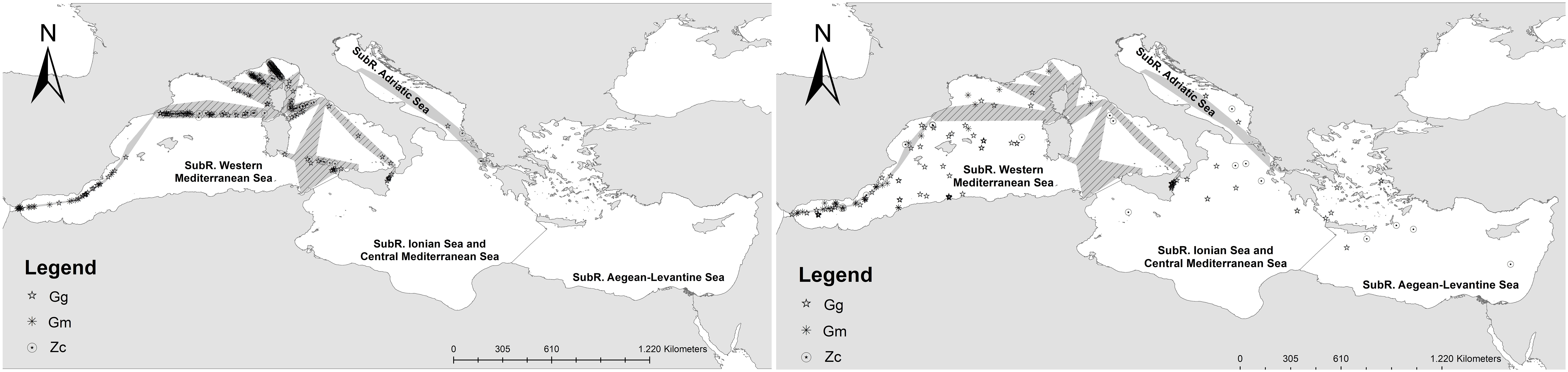
Figure 2 Dataset used for model building (left) and independent dataset used for validation (right).

To calculate the extent of suitable area (Ecological Potential Range, EPR), the output binary suitable-unsuitable predictions rasters were converted into polygon layers including the highest suitable class for each species and period and were then used to measure the EPR in km². Then, the percentage difference in the EPR between periods was calculated for each species as: [(EPR_{(2nd period)} - EPR_{(1st period)})/EPR_{(1st period)})].

2.3.3 Range pattern

The trend in distributional pattern was calculated in terms of shift either in the surface or in the centre of gravity (centroid) of range areas (ODR, EPR), assessing the: a) overlapping area between the two periods (for the ODR considering only the common effort area between the two periods); b) percentage of overlapping area compared to the first period calculated as [(Overlapping area/Area 1st period)*100] and c) direction and magnitude of shift in the centroids of the range area between the two periods (calculated through the geometric spatial zonal statistic in GIS).

2.3.4 Observed distributional range vs ecological potential range, ODR/EPR

The proportion of the suitable habitat effectively occupied by the species (ODR vs EPR) was calculated for each period considering only the areas covered by the effort identified by the MaxEnt bias files. Within these areas, the extent of suitable habitats (Ecological Potential Range, EPR) was estimated in km². The percentage proportion of the predicted EPR occupied by the species (ODR) was calculated as: [(ODR/EPR) * 100], and differences between periods were computed as: [(%_{(2nd period)} - %_{(1st period)})/%_{(1st period)})]

3 Results

During the twelve years between 2008 and 2019, the FLT Med Net covered almost 500,000 km of effort and recorded 296 sightings of Gg (86), Gm (68) and Zc (142). Group sizes of the species were not significantly different between the two periods, but they differed among species: Gg groups were composed by a mean of 5 individuals (5.7 ± 5.1 SD_{1st period}/4.7 ± 4.3 SD_{2nd period}), while Gm groups were generally larger (7.0 ± 9.5 SD_{1st period}/7.0 ± 6 SD_{2nd period}), and Zc smaller (mean group size of 1.67 ± 1.0 SD _{1st period}/1.87 ± 1.2 SD_{2nd period}).

3.1 Observed distributional range, ODR

The area covered by the effort was the largest in the WMED Subregion, while very limited in the Central MED during the first period (i.e., eastern Sicily), and increased during the second thanks to the inclusion of new Adriatic routes covering also the Northern Hellenic Trench (Figure 1). No effort was performed in the Aegean-Levantine Subregion (Table 1).

Table 1 Distribution and extent (in km²) of the area of effort per each Mediterranean Subregion, extent of observed species range calculated within the 95% KDE isopleth, and percentage of overlap between observed species range and effort area.

Between 10 to 37% of the effort area overlapped with the species observed range (ODR) in the WMED. In the Central MED instead, 99% of the effort area overlapped with Gg ODR during the first period (i.e., in the eastern Sicily), and a limited percentage with the ODR of Zc (2%) during the second period (i.e., in the Northern Hellenic Trench). In the Adriatic, 7% of the effort area intercepted the Gg ODR in the southern part.

ODR areas were mostly located in the northern part of the WMED Subregion for all the species (Figure 3) with ODR for Gg also located in the westernmost MED, the Tyrrhenian-Sardinian channel and the southern Adriatic, Gm in the westernmost MED, and Zc in the eastern Ionian (i.e., Northern Hellenic Trench). In the northern area, the ODR generally overlapped between the two periods, with a tendency to shift towards offshore in the Sardinian-Balearic basin for all the three species, and in the Ligurian Sea for Gg (Figure 3, left).

Figure 3 Core areas highlighted by the 95% KDE isopleth within the area covered on effort during the two periods (in grey), used to define the Observed Distributional Range, ODR (Gg left, Gm centre, Zc right).

Considering only the common area of effort between the two periods, the trend calculated over the ODR extents revealed an expansion in all the three species with a significant delta index >10% for Gg (+16%).

3.2 Ecological potential range, EPR

Based on AUCs, validation data, and well-known sites of species presence, model outputs showed strong predictive skill at the basin wide scale. The ROC plots exhibited high average AUCs for both training and test datasets and small Standard Deviation and overfitting values for all models (Table 2), which indicates consistency and reliability. In general, performance of the prediction maps of the second period was higher compared to those of the first period when validated by the independent dataset collected during the same period. Performance was also higher for prediction maps for Gm2 (over 90% of correct prediction), while performance of Gg and Zc maps was fair-good in the WMED Subregion only (over 70% of correctly predicted sites).

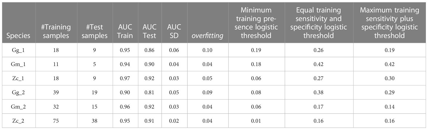
Table 2 MaxEnt Results for the first and second periods considered.

In general, the areas of suitable habitats highlighted by the MaxEnt output maps were consistent with previous knowledge on the species (Figure 4) with the highest incongruence noted for the Gm_2 prediction in the Aegean-Levantine Subregion. Standard Deviations were generally low (<0.4), especially for the unsuitable areas. However, uncertainty was highest in general in the Aegean-Levantine Subregion and in the central and southern areas of the Central MED Subregion for the Gg_1 and Zc_2 outputs.

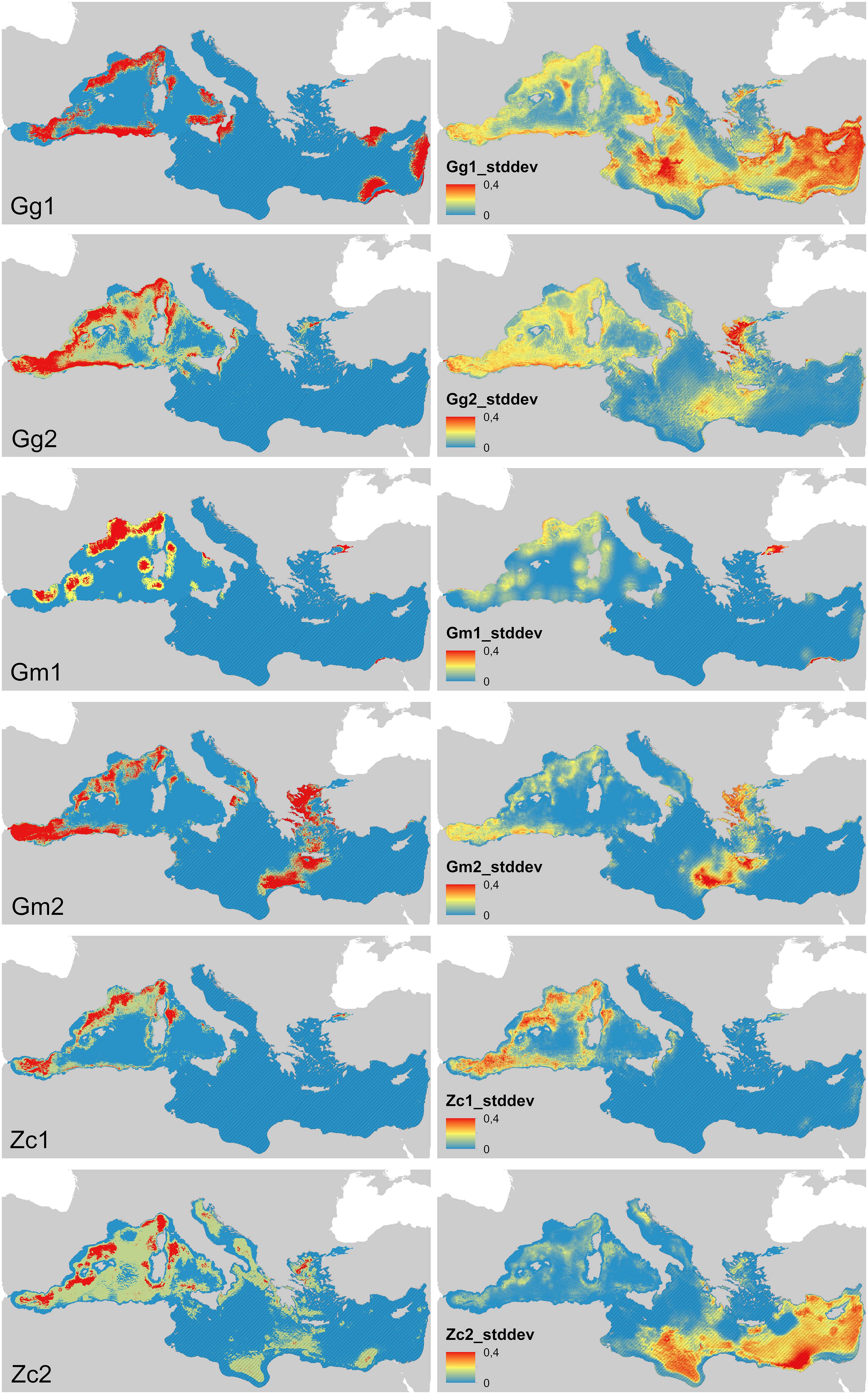
Figure 4 Output of the Suitable Habitats predicted based on 2008-2012 (Gg_1, Gm_1, Zc_1) and 2013-2019 (Gg_2, Gm_2, Zc_2) FLT Med Net data (left) with the relative Standard Deviation (right). The partition of suitable habitat is shown under three threshold scenarios defined by: ‘Equal training sensitivity and specificity logistic threshold’ (red), ‘Minimum training presence logistic’ and ‘Maximum training sensitivity plus specificity logistic threshold’ (values in Table 2). Blue colour displays the predicted unsuitable habitat. Striped lines identify the Subregions where the prediction must be considered with caution as based on limited or no effort.

The ‘Minimum training presence’ threshold produced binary maps restricted to the most suitable habitat only excluding a large number of presence sights. The values identified through the ‘Equal training sensitivity and specificity’ and ‘Maximum training sensitivity plus specificity’ thresholds resulted similar (Table 2), but the first approach was chosen as being more conservative and was then used to define the EPR.

Some differences in the EPRs were found between the two periods (Table 3) in the WMED, where the EPR of Gg decreased by almost -7%, while Gm increased by 57% and Zc by 4%. Results for the other Subregions were not reliable as they were based on very small probability of presence in those areas (<5000 km²).

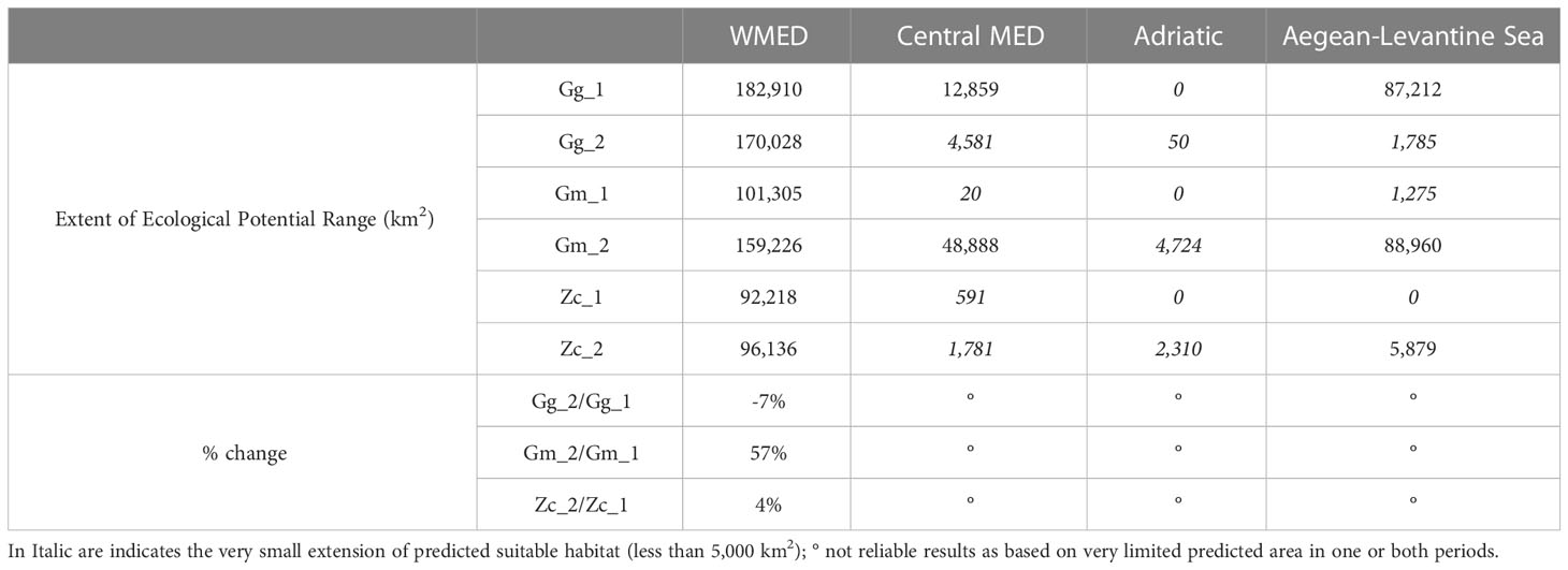
Table 3 Extent area of potential range (EPR, km²), based on Equal sensitivity plus sensitivity logistic threshold and percentage of change in the extent of suitable area (2008-2012: Gg_1, Gm_1, Zc_1; 2013-2019: Gg_2, Gm_2, Zc_2).

In general, Distance from Canyon, Chl-a, and depth were the most important predictors for all the three species, followed by seamount distance and SST, but only for Gm and Zc (Table 4). Chl-a was the most important parameter for the definition of Gg habitats, either as percent contribution or permutation importance, in both periods, followed by canyon distance during the first period and depth during the second. Distance from Canyon was the most relevant parameter for Gm during the first period, while Chl-a strongly contributed during the second period, followed by the distance from seamounts. Chl-a and distance from canyon were the most significant parameters also for Zc during the first period, while depth and distance from seamounts were the parameters that most affected the distribution of the species during the second period.

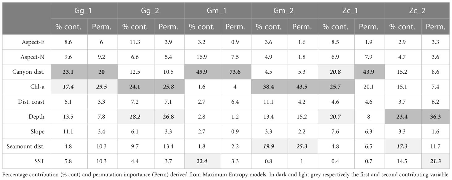
Table 4 Measures of environmental variables contribution to the ecological models for the target species.

3.3 Range pattern

In addition to the investigated changes in the extent of range areas, the analysis of spatial pattern revealed some shifts in the location of the main range areas. Indeed, the percentage of overlapping spanned 40-70% for ODR for the three species reaching the maximum overlap for Zc, and 30-50% for EPR. The location of overlapping areas for ODR (Figure 3) and EPR (Figure 5) showed the permanence over the time of some well-known areas for the three species.

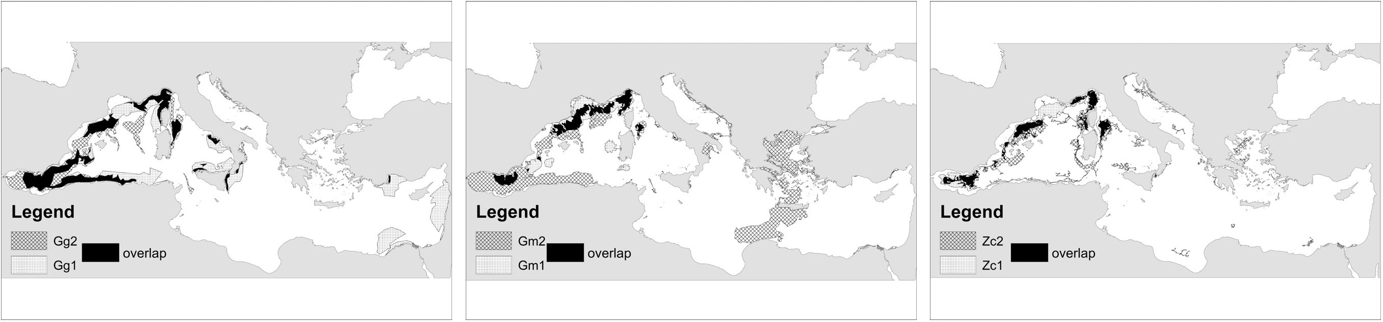
Figure 5 Overlap of EPRs over the two periods. Points EPR of the first period, strips EPR second period, and in black the overlapping areas.

In particular for Gg, some well-known areas of the WMED were predicted in both periods (e.g., Alboran Sea, Balearic Sea, Corso-Ligurian-Provençal basin, several spots in Tyrrhenian Sea including the Pontine Archipelago, and eastern Sicily). The offshore waters of the Gulf of Lion were no longer identified as the most suitable during recent years, while some new areas emerged (Figures 4, 5). A general reduction of suitable habitat was identified in the Pontine Archipelago and around the Sicilian coasts. Other widespread spots of potential suitable habitat appeared dispersed in the WMED from the recent model. Outside the more reliable area of the WMED, some suitable areas with higher uncertainty emerged in the eastern Mediterranean basin such as the southern Türkish, the northern Aegean during the more recent period and the coasts between Lebanon and Egypt.

Suitable Gm habitats were predicted in the WMED Subregion, in the Alboran Sea and along the continental shelf of Balearic, Gulf of Lion and the Corso-Ligurian-Provençal basin. A small area was highlighted in the Pontine Archipelago, and other patch areas were predicted around Sardinia Island. During the second period, new ODR areas were identified over the Alboran Sea and the Strait of Gibraltar due to the added effort in this region which intercepted the known important areas for the species identified by the large EPR. Outside the WMED, the large prediction stretching from the Aegean to Libya seems unreliable given the current knowledge on the species distribution.

Some well-known suitable areas were highlighted in both periods for Zc in the WMED such as the Alboran Sea, Ligurian Sea, northern Tyrrhenian Sea, and Balearic Sea. In the Central MED and Adriatic Subregions, the Hellenic Trench, northern Ionian Sea, and southern Adriatic Sea were predicted during the second period only with higher uncertainty.

A shift of centroids’ core areas between the two periods was detected for the ODR and the EPR predicted over the WMED Subregion (Figure 6). The shift on EPR for the other Subregions or at all MED scale was not considered as based on a very limited predicted area in one or both periods (Table 3).

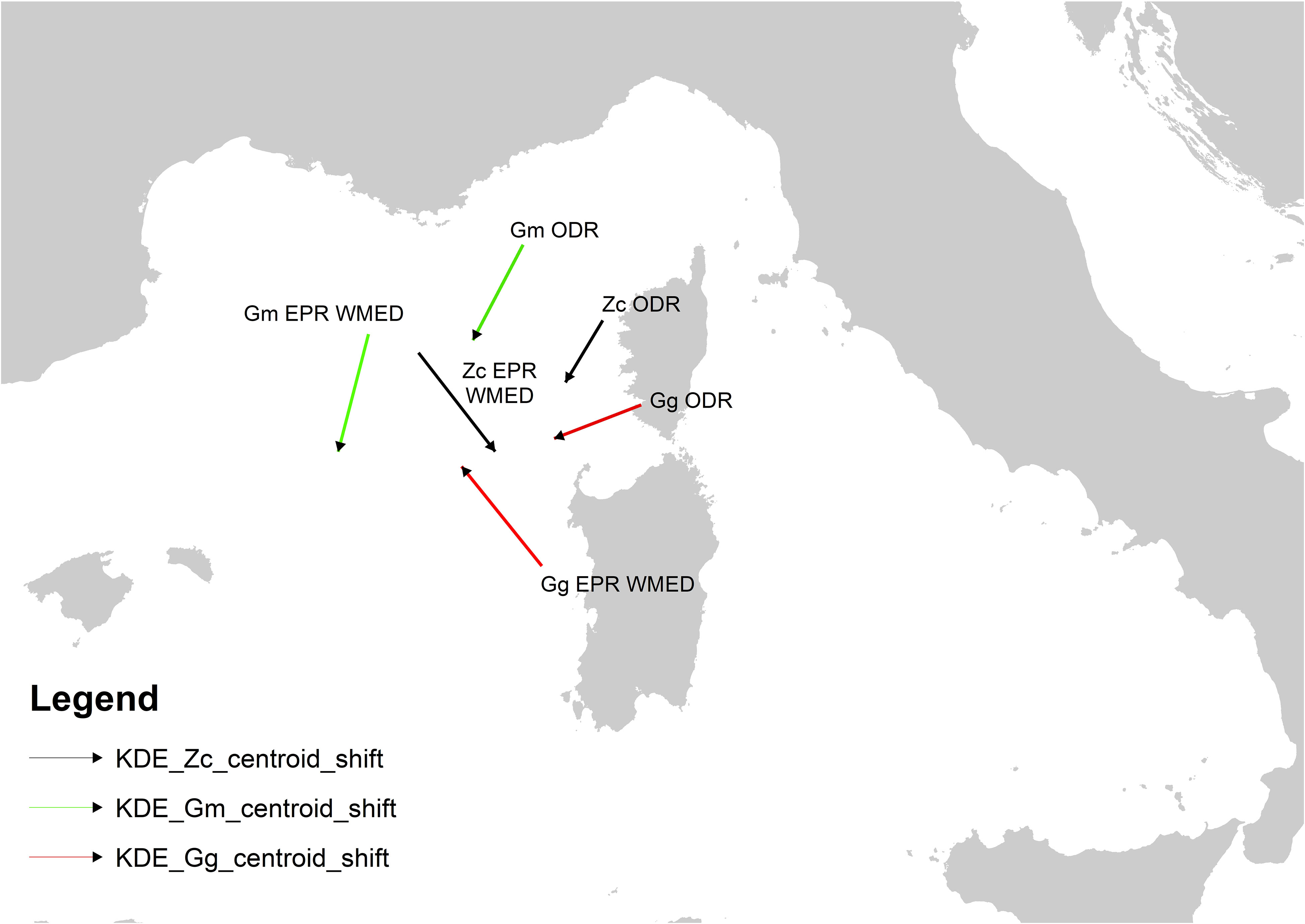
Figure 6 Direction and magnitude shift of the centroids of the distributional area respectively of ODR, and EPR WMED. Gg red, Gm green, Zc black lines.

3.4 Observed distribution range vs ecological potential range, ODR/EPR

Results showed that all the species regularly occur in almost the same areas or in a smaller proportion of their ecological potential habitat during both periods (ODR equal or smaller than EPR), with the only exception of Gg, whose ODR in the second period was larger than the EPR (Table 5, SM Figure 1). In the WMED, the proportion of suitable habitat effectively occupied by the species ranged between 62% for Gm_1 and 158% of Gg_2. No significant changes were detected in the proportion of occupied vs potential habitat over the two periods for the Zc (-1%), while for Gg and Gm increased this proportion by 59% and 46% respectively. Limited area was predicted for Gg and Zc in the Central MED, effectively occupied by the Zc by 50%, while the Gg was recorded largely outside the predicted potential area. Gm was never detected either in the surveyed areas of the Central MED or in the Adriatic Subregions. The spatial pattern of observed and predicted potential areas showed large overlap, but with some local differences (SM Figure 1). Both the areas of observed and predicted range of Gg in the northern part of the WMED expanded mainly towards offshore waters and stretched in patchy suitable areas in the centre. However, the shift in ODR detected in the more recent years in the western portion of the Corso-Ligurian-Provençal basin brought Gg outside predicted suitable areas. A contraction in suitable areas was instead detected in the south Tyrrhenian, where the species was no longer present, while new areas emerged in the Sardinian channel. A suitable area was confirmed in eastern Sicily in both periods. Gm observed range was almost similar across periods in the northern WMED, except for an enlargement towards offshore waters in the Sardinia-Balearic basin, which almost corresponded with the predicted potential range despite the latter being more scattered and fragmented during the more recent years. On the other side, a relevant area potentially suitable for Gm was revealed in both periods not overlapping any ODR in the central Tyrrhenian Sea. No noteworthy changes in observed and predicted range were detected for Zc in the northern part of WMED, while a new area emerged in the Sardinian channel both for the observed and predicted range.

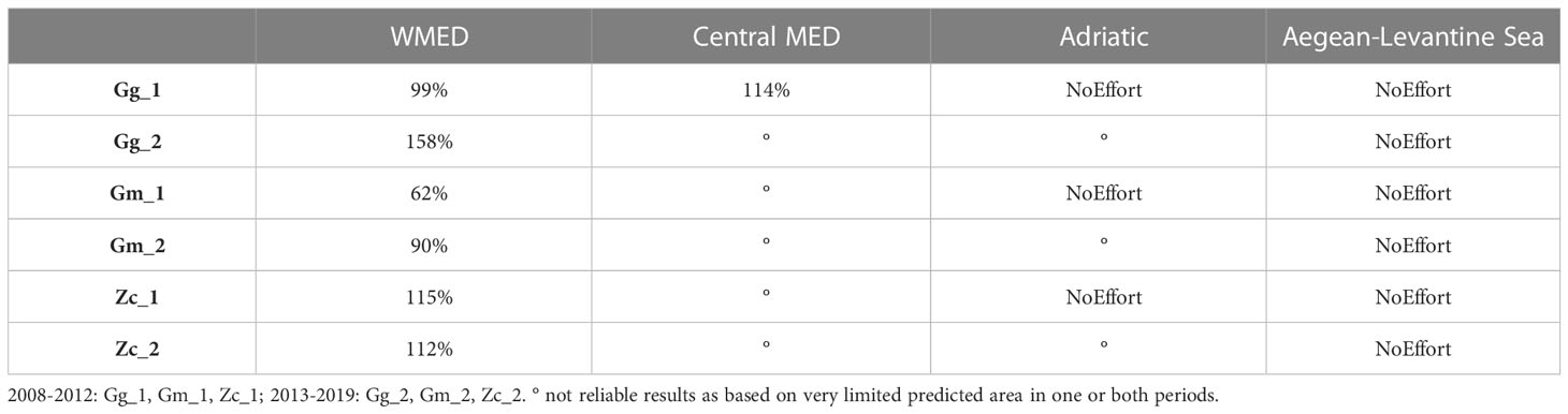
Table 5 Percentage of the extent of Real Distribution (km², 95% KDE isopleth) over the Ecological Potential Range (km², based on Equal sensitivity plus sensitivity logistic threshold) calculated within the area performed on effort.

4 Discussion

4.1 Sampling strategy

The sampling strategy of the FLT Med Net was set in order to homogeneously cover large portions of the Mediterranean basin, with regular monitoring of the sampled areas during all the seasons (Arcangeli et al., 2019). A recent study revealed that sampling designed along multiple fixed ferry routes detected more species and were able to recover known patterns in species richness and distribution at smaller sample sizes better than unconstrained sampling points (Boyse et al., 2023). Results of this study confirm that the sampling design of the FLT Med Net proved adequate for catching the known distribution of the species, providing high modelling performance, and allowing trends analysis even for rare or elusive cetacean species such as Risso’s dolphin, long-finned pilot whale and Cuvier’s beaked whale. This was particularly the case for the WMED Subregion, and especially during recent years when new monitored transects also covered the westernmost portion of the basin, the Alboran sea and the Strait of Gibraltar area (roughly 80% of WMED covered by the effort). In the Adriatic Subregion, the effort strategy resulted in coverage of almost the whole region although with still some uncertainty in the northernmost area, as also assessed by Zampollo et al. (2022). The Central MED was instead only represented by the effort in the eastern Sicilian coast and the Greek Ionian portion, and no effort was performed in the Aegean-Levantine Subregion, which leaves open opportunities for improvement. Indeed, an adequate proportion of the effort area intercepted the main distributional range and suitable habitats of Gg, Gm and Zc in the WMED Subregion (between 10-37% for the observed distributional range, over 46% of the predicted ecological range), and a more limited proportion in the Central MED and Adriatic Subregions, in correspondence with some known important areas for Gg (i.e., eastern Sicily. e.g., ACCOBAMS, 2021) and Zc (i.e., Northern Hellenic Trench, e.g., Frantzis et al., 2003). Therefore, in the WMED the sampling design of FLT Net proved to be adequate to intercept the ecological variability of the area, producing reliable results also outside the area of effort, whereas more transects are instead required to improve reliability in understudied Subregion (e.g., Central and Aegean-Levantine Subregions). Moreover, as the distributional range and habitat use of species varies seasonally, the seasonal based temporal resolution of sampling strategy allowed including the potential seasonal displacement of the species and thus the entire species range. The approach was also effective in terms of monitoring costs vs. acquired information, and these methods and indicators are suitable to be replicated across all seas.

4.2 Main findings on species distributional range and habitat

Most of the Observed Distributional Range (ODR) of the species highlighted by the Kernel analysis and the Ecological Potential Range (EPR) predicted on the basis of suitable habitat modelling were consistent with previous knowledge on the species, especially for the WMED Subregion, further confirming the importance of the north-western Mediterranean for Gg, Gm and Zc (ACCOBAMS, 2021). Consistency in these areas was also found across periods, with a general enlargement in the areas of distribution, and a shift towards more offshore areas in the Sardinian-Balearic basin for the three species, and in the Ligurian Sea for Gg. Outside the WMED, some known important areas for Zc such as the Ionian Sea and the deep Hellenic Trench were predicted, even if for a limited extent, during the second period only, when monitoring effort was added in the Adriatic-eastern Ionian region. Higher uncertainties or unreliable areas were revealed, as expected, in unsurveyed areas of the Central or the Aegean-Levantine Subregion.

Findings of this study on both ODR and EPR of Risso’s dolphin (Gg) confirmed the permanence across the two investigated periods of some well-known important areas for the species in the WMED Subregion. The species is mostly found in the Western-Mediterranean Sea from the Alborán Sea, including deep offshore waters (Cañadas et al., 2002; Cañadas et al., 2005), to the south of the Provençal basin, with high values along the Algerian coast and the Balearic Islands (ACCOBAMS, 2021; Lanfredi et al., 2021). However, findings of this study no longer identified the offshore areas of the Gulf of Lion as most suitable during recent years, while highlighting new distributional areas in the offshore waters of the Sardinian-Balearic basin and Ligurian Sea. The species was considered favoured by the proximity of the continental slope, primarily in the north-western basin (Bearzi et al., 2011), with a very specialised niche and a habitat spatially restricted on the upper part of the continental slope (Praca and Gannier, 2008). A high fidelity for the Provencal continental slope, without strong seasonal pattern in abundance (Laran et al., 2010; Laran et al., 2017), and a transient use of the offshore area was also confirmed on a long-term basis between 1989-2012 by Labach et al. (2015). Nonetheless, during recent years Gg was sighted in more offshore environments than previously reported in literature (ACCOBAMS, 2021). This is also in line with the trend observed by Azzellino et al. (2016), who reported a significant decrease in Gg abundance between the early ‘90s and 2014 in coastal and continental slope areas of the Ligurian Sea, with stable occurrence in pelagic areas. The result was assumed as a loss of coastal group or a shift in animal distribution (Azzellino et al., 2016). Moreover, apart from the more defined sites, widespread spots of potential suitable habitats appeared dispersed in the WMED in the current study. A general reduction of suitable areas was also detected in the Pontine Archipelago, and around the Sicilian coasts and Ionian Sea, where only a portion of suitable habitat persisted eastern of Sicily and Taranto Gulfs where strong side fidelity was found by other studies (e.g., Monaco et al., 2016; Carlucci et al., 2020a; Cipriano et al., 2022). Relatively large groups of Risso’s dolphins were reported further east in the southern Adriatic and Ionian Seas and the deep Hellenic Trench from ASI visual surveys, but no sightings were reported from acoustic surveys (ACCOBAMS, 2021) in line with the uneven prediction produced by this study. During the first period, some suitable areas emerged in correspondence of the Türkish Mediterranean, Palestinian and Israeli coasts consistent with the few contemporary reports (Öztürk et al., 2011; Kerem et al., 2012). The absence of effort in this area prevents any conclusion on whether or not the predicted reduction reflects a true species negative trend. The few encounters of Gg in mixed-species groups with striped dolphins and short-beaked common dolphins in the deep waters of the semi-closed Gulf of Corinth (e.g., Frantzis and Herzing, 2002; Frantzis et al., 2003), and for the unique stranding record in the 2012 in the Marmara Sea (Dede et al., 2013) appear to confirm the minor prediction in these areas.

Findings of this study confirmed some of the existing knowledge on the long-finned pilot whale (Gm). The species is known to be found almost exclusively in the WMED (Verborgh et al., 2016; ACCOBAMS, 2021) with a strong preference for deep pelagic waters. Relative higher densities were reported in the Strait of Gibraltar and Alboran Sea (Cañadas et al., 2005; De Stephanis et al., 2008) and lower in Balearic and Corso-Ligurian-Provençal Seas (Raga and Pantoja, 2004; Gómez de Segura et al., 2006; Azzellino et al., 2008; Praca and Gannier, 2008). The ACCOBAMS survey of 2018 (ACCOBAMS, 2021) also observed larger groups of Gm in the Alborán Sea, along the coast of Morocco and in the Gulf of Lion, and relatively smaller pods in the Ligurian Sea. The species was never recorded in the central Tyrrhenian Sea (Arcangeli et al., 2013; Arcangeli et al., 2017), but a stable pod has been recurrently sighted in the Pontine Archipelago since 1995 (Mussi et al., 2000). In accordance with the literature, the ODR in this study for Gm was exclusive of the WMED, but with a tendency to shift towards offshore waters during recent years, especially in the Sardinian-Balearic basin. Suitable habitats were also mostly predicted in the Alboran Sea and along the continental shelf of the Balearic Archipelago, Gulf of Lion and the Corso-Ligurian-Provençal basin with a similar shifting trend towards offshore as the Observed Range. Smaller areas were predicted in the Pontine Archipelago, supporting the stable presence reported by Mussi et al. (2000), and around Sardinia Island. In the Tyrrhenian Sea instead, a relevant potentially suitable area was highlighted during both periods, although no sightings have been reported either from this study or by literature (e.g. Arcangeli et al., 2017). Further investigation could be directed to determine whether anthropogenic activities or other pressures are operating there as limiting factors for the species. During the second period, a reliable enlargement of suitable habitat was predicted in the WMED Subregion, especially over the Alboran Sea and the Strait of Gibraltar, most likely as a result of the new added monitored transects representative of the westernmost part of the basin and intercepting the Strait of Gibraltar sub-population (Verborgh and Gauffier, 2021). A large Ecological Potential area stretching from Gibraltar towards the northern African coast was indeed predicted by this study in the second period, consistent with the ACCOBAMS (2021) sightings of large pods and by some reported strandings in Morocco (Bayed, 1996; Masski and De Stephanis, 2018), Algeria (Boutiba, 1994; Bouslah, 2012) and Northern Tunisia (Attia El Hili et al., 2010; Karaa et al., 2012). The species was never detected either in the Central MED and in the Adriatic Subregions, and no EPR was predicted here, while the large prediction stretching from the Aegean to Libya seems unreliable given the current knowledge on the species distribution.

Known habitats of Cuvier’s beaked whale (Zc) were highlighted by the study in the WMED Subregion, while the south Adriatic and Hellenic Trench of the eastern Ionian Sea were only predicted during the second period likely due to the effort performed in those areas that allowed including some environmental features not considered by the environmental variability of the WMED effort area only. Zc is considered to inhabit both the western and eastern basins of the Mediterranean Sea (Podestà et al., 2016), and this species is mostly found in canyon areas in the Ionian Sea, the Hellenic Trench, the deep southern Adriatic Sea (Frantzis et al., 2003; Carlucci et al., 2020b), the central Tyrrhenian Sea (Gannier, 2015; Arcangeli et al., 2016), the Balearic and the Alborán Seas (Cañadas and Vázquez, 2014; Cañadas et al., 2018), and the Ligurian Sea (Moulins et al., 2007; Azzellino et al., 2008; Tepsich et al., 2014). The ACCOBAMS survey of 2018 confirmed the existing knowledge on the basin wide presence of the species and at the same time showed how Zc occur in relatively small patches at low densities (ACCOBAMS, 2021). In accordance with literature, this study highlighted the importance in particular in the WMED of the Alboran Sea, the central Tyrrhenian Sea and Ligurian Sea and also a permanent area of suitable habitat in correspondence with the Spanish-French continental slope coast and stretching offshore. However, despite being recognised by some studies (Raga and Pantoja, 2004; Gannier and Epinat, 2008; Praca and Gannier, 2008; Podestà et al., 2016; Arcangeli et al., 2017) and the records of the Accobams survey (ACCOBAMS, 2021), this latter area was not considered among the important areas for the species. This discrepancy could indicate either an underrepresentation of scientific literature or a minor occupancy of Ecological Potential habitat for the species.

4.3 Interpretation of trends

In general, the persistence over time of presence and suitable habitat of Gg, Gm and Zc in the WMED confirmed the importance of this Subregion for the species. However, the changes in the extent (whichever a contraction or expansion) and the shift highlighted on both the observed distribution and the suitable areas indicate changes in spatial distribution of the species across time periods (Table 6). This could be the result of exploitation of new potential suitable areas or an adaptation forced by existing pressures or changes in the distribution of habitat over time. In particular Gg enlarged the proportion of occupied area over the ecological potential by almost 50% distributing also outside the predicted suitable areas (i.e., in the Corso-Ligurian-Provençal basin). In addition, the new areas that emerged in the centre of the Sardinian Balearic basin or eastern Corsica coast, together with the contraction of the areas in the south Tyrrhenian Sea and around the Sicilian coasts, revealed changes that need further investigation. Moreover, results highlight a concurrent enlargement of the area of distribution of Gm and Zc, even if for a minor extent, that is not yet reported by other studies. If confirmed, this would be a signal of a general tendency towards a more dispersed distribution that surely deserves attention.

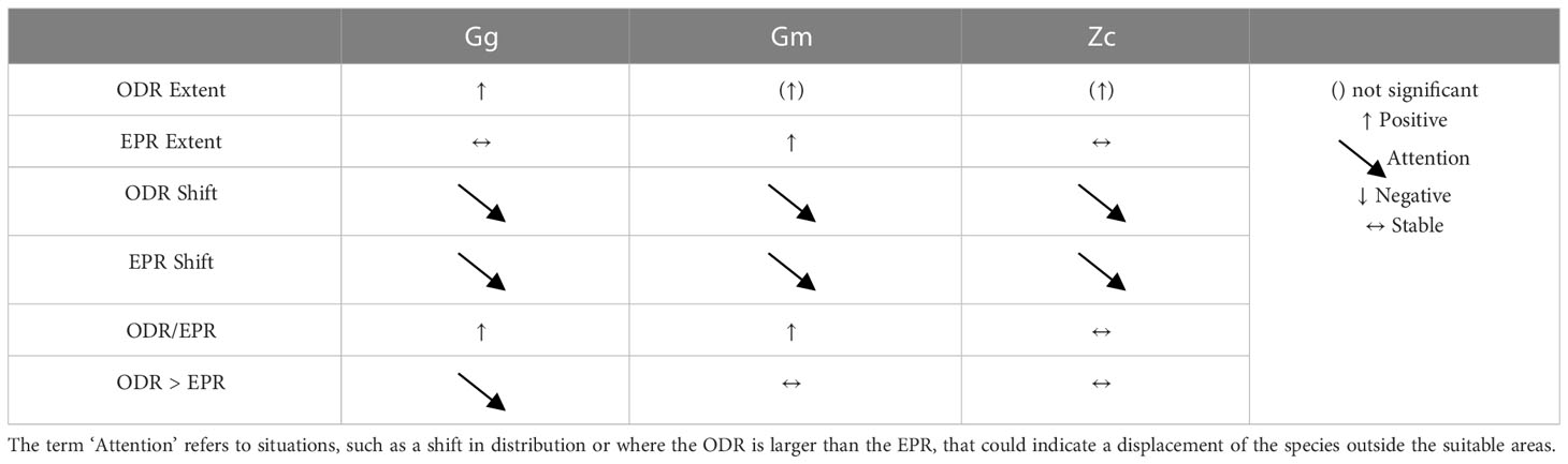
Table 6 Summary results on assessed trends for the WMED Subregion.

4.4 Methodological approach and indicators

The indicators here tested helped to describe the main consistencies or changes in short-term range trends between periods. Results highlighted the advantages and weaknesses of each indicator and of the approach tested.

The Observed Distributional Range (ODR) indicator has the advantage of preventing difference biases by data processing, analysis settings or approximations and is closely related to the real observed distribution of the species. On the other hand, results are only representative of the area where the effort is performed, introducing the need for specific planning of the sampling design of the data collection if used as representation of species distributional range. Spatially extensive surveys covering the whole range of species would deliver an adequate baseline for detecting ODR, but they are cost-expensive and may lack the temporal resolution needed to detect the natural species variability avoiding output linked to occasional or seasonal fluctuations. Continuous local scale surveys could provide long-term series but lose the spatial representativeness. Local and large scale surveys could be merged to increase the spatial representation of outputs providing that appropriate metric is used to match data collected with different methodologies. Time extensive large-scale monitoring data collected in sampled areas spatially representative of regional ecological conditions could represent a suitable balance and can be used as an index of the real species range. A prior assessment of the ecological variability representativeness of monitored transects is needed to avoid bias in underrepresented regions.

With regard to the methods to represent the distributional range, if compared to the species occurrence mapped in a 10 x10 km² grid as suggested by HD and MSFD, the Kernel density smoother proved to be a feasible tool to spatially generalize the distribution of species and define the area where the species is found. It is adaptable to the spatial scale (grain) and resolution of data through the adjustment of search radius and cell size resolution while still remaining relatively simple to apply. Moreover, when using high quality spatial data as those of this study, the use of KDE could be considered as more accurate than other coarser methods such as grid of occurrence or the Minimum Convex Polygon used by some EU Member States. Other approaches such as the Kriging could also apply to the same purpose and are worth exploring.

Finally, care must be taken when calculating the trend in the extent of ODR in cases when the monitored area changed between time periods. In this study, the trend was calculated as percentage of change of ODR vs Extent of Effort (i.e., it was normalised by the Effort), and the percentage of change didn’t vary if considering the entire effort areas for each period or the common area only. However, the second approach was chosen as more conservative. Indeed, a change in the investigated area could produce a bias if, for example, an area completely outside, or, vice versa, in the core of the species range, is surveyed during one period only. Given the long-term monitoring required by the legislative framework at the large-range spatial scale needed for cetacean species, changes in the monitored areas over time could occur for example in the case of new organisations or countries joining an international effort. This aspect should be carefully considered, and the trend detected should be investigated with a conservative approach within the common effort area only.

The Ecological Predicted Range (EPR) based on sites of known occurrences and extrapolated through habitat maps models proved to be able to generalize the spatial distribution of the species also outside the area of effort providing meaningful outputs especially in the WMED Subregion where sampling was spatially representative of regional ecological conditions. Results of this study further confirm that sampling effort must be designed in order to assure representativeness of the regional ecological variability, and the SDM outputs in not surveyed regions (e.g., as in the case of the Aegean-Levantine basin in this study) should be taken with caution. In addition, predictions and extrapolations should be validated whenever possible by independent datasets as soon as new data become available. Results of this study indicate a general correspondence of trends detected in the Observed and Predicted Range both in terms of shifts (e.g., towards offshore areas in the Western-Mediterranean Subregion for all the species) and extent of areas (e.g., enlargement recorded for Gm in both ODR and EPR). These results confirm the potential for using the EPR to indirectly determine the AOO as suggested by the IUCN Guidelines (IUCN, 2001). However, some differences were also detected such as the new areas detected by the ODR in the Sardinia channel for Gg that were not predicted by the EPR in the corresponding period. Thus, careful consideration is needed to correctly discriminate the meaning of the range predicted on the basis of SDM to investigate the species conservation status, as the Potential Range does not always correspond to the actual distributional range of the species. Output must be carefully validated and adjusted using the estimated proportion of ODR/EPR as suggested by IUCN (2001).

On the other hand, Suitable Habitat Maps can be directly used to define the extent, trend and pattern of the suitable habitats to answer the parameter/criteria ‘Habitat’ for the species (e.g., for HD and MSFD). By including information on the main ecological factors that drive their distribution, these models can also be used to investigate the “Habitat conditions” requirement if the pressures are added to the models.

Provided SDMs accurately reflect potential ranges, EPR can also be used to compare the Observed versus the Potential Range (IUCN, 2001; IUCN, 2022) as they indicate the area of occupied habitat and describe unoccupied habitats of suitable quality allowing the long-term survival of the species (DG ENV, 2017). If appropriate data are available, the comparison between the Observed and the Potential Range can also help to identify potential suitable areas that are not used by the species due to the influence of anthropogenic pressures or other limiting factors. Alternatively, EPR can also be used to determine if the species is pushed outside of the preferred suitable habitat as a consequence of a pressure, change in the distribution of habitat or the exploitation of new resources. Trend in the ratio between Observed vs Potential range could then be used to correlate the detected changes with other environmental or anthropogenic parameters and/or assess the effectiveness of mitigation measures.

5 Conclusions

Our results highlighted the strengths and weaknesses of the analysed indicators and approach as summarised in Table 7. In general, the ODR based on known occurrence can underestimate the real occupied range and needs to be referred to the area of effort, but it can still be used as an index to detect trends. Conversely, the EPR could be larger than the occupied range in presence of limiting factors, either environmental or anthropological, or even smaller in the case of pressures that force the species outside the ecological niche so that careful validation of output is required. Therefore, the parallel use of complementary indicators, such as the Observed and Ecological Potential Range, may be preferable to using a single indicator to disclose the significance of a change.

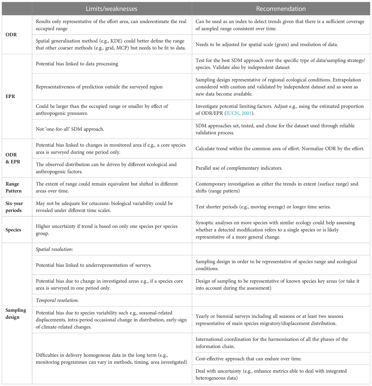
Table 7 Summary of limits/weaknesses of the indicators and approach tested, and recommendations.

Based on our results, we also recommend the contemporary investigation of the Range Pattern as either the trends in extent (surface range) and shifts (range pattern). In this study, for example, the enlargement of the Observed surface Range could have been interpreted as positive, but it was associated with a shift towards offshore less suitable or unsuitable areas which instead deserve attention. Moreover, synoptic analyses performed on more species with similar ecology are suggested to assess whether a detected modification refers to just a single species or is likely representative of a more general change.

This study tested and discussed the most common approaches for assessing six-year trends, as required by the HD and MSFD, on range and habitat of rare cetacean species using the longest dataset available at large scale in the Mediterranean Sea. It should be noted that the comparison between two six-year periods may not be adequate to highlight biological and ecological trends for such long-lived species as cetaceans. Biological variability could indeed be revealed under different time scales, and further investigation, such as a moving average of shorter periods or longer time series, might be necessary to confirm the usefulness of the six-year time frames required by the legislative framework or to propose more appropriate time periods.

Overall, our analyses also contribute to assess the most effective methods to evaluate the Range and Habitat indicators in compliance with the international legislative requirements of, among others, the HD, MSFD, and Barcelona Convention.

Data availability statement

The data analysed in this study were collected by several organisations participating in the FLT Med Net. Each organisation owns the data collected. Requests to access these datasets should be directed to the data owners listed in Supplementary Table 1.

Ethics statement

Ethical review and approval were not required for this study as the research was conducted solely by non-invasive collection of visual record from a passenger ferry. Animals were not approached by the vessel, and data were collected in passive mode approach.

Author contributions

AA conceptualisation of theoretical framework, design of methodology, performed formal analysis, writing and editing of the manuscript. AO Methodology for spatial distribution modelling. MA, LD, and PT contributed in the conceptualisation of theoretical framework; Data Curation; Writing - Review & Editing. IC, LB, OG-G, MG, AS, MV, and LC Data Curation, Writing - Review & Editing. RC contributed to the conceptualisation of the theoretical framework, Review & Editing. FA Help manage and supervise the project. All authors contributed to the article and approved the submitted version.

Funding

The project was conducted within the FLT Med monitoring Network programme runs with self-found by the partners and was partially funded during the years by a number of projects such as MEDSEALITTER, Interreg Marittimo IT-FR SicomarPLUS, France MSFD, Pelagos France. The analyses performed for this study were conducted in the framework of the Life CONCEPTU MARIS Action A2 (NAT/IT/001371).

Acknowledgments

The authors would like to thank students and interns from the CETASMUS program and Accademia del Leviatano, all the observers that helped collecting the data and in particular the people that greatly helped with the logistic coordinating over time such as Miriam Paraboschi, Giuliana Pellegrino, Marine Roul. A special thanks to all the Ferry companies participating in the programme and hosting the researchers onboard and in particular Corsica-Sardinia Ferries, Grimaldi lines, Minoan, Tirrenia and Baleària. A special thanks to C. Pizzutti and Paul Kyprianou for their constant support. The authors are grateful for the availability of data used as independent dataset for the validation of the models, and in particular to Clara Monaco (Ketos-Marecamp), Sally Hamilton (ORCA) and ACCOBAMS.

Conflict of interest

The authors declare that the research was conducted in the absence of any commercial or financial relationships that could be construed as a potential conflict of interest.

Publisher’s note

All claims expressed in this article are solely those of the authors and do not necessarily represent those of their affiliated organizations, or those of the publisher, the editors and the reviewers. Any product that may be evaluated in this article, or claim that may be made by its manufacturer, is not guaranteed or endorsed by the publisher.

Supplementary material

The Supplementary Material for this article can be found online at: https://www.frontiersin.org/articles/10.3389/fmars.2023.1116829/full#supplementary-material

References

ACCOBAMS (2021). Estimates of abundance and distribution of cetaceans, marine mega-fauna and marine litter in the Mediterranean Sea from 2018-2019 surveys. Eds. Panigada S., Boisseau O., Canadas A., Lambert C., Laran S., McLanaghan R., Moscrop A. (Monaco: ACCOBAMS - ACCOBAMS Survey Initiative Project), 177.
Arcangeli A., Aissi M., Atzori F., Azzolin M., Campana I., Carosso L., et al. (2019). Fixed line transect mediterranean monitoring network (FLT med net), an international collaboration for long term monitoring of macro-mega fauna and main threats fixed line transect mediterranean monitoring network. Biol. Mar. Mediterr 26 (1), 400–401.
Arcangeli A., Campana I., Bologna M. A. (2017). Influence of seasonality on cetacean diversity, abundance, distribution and habitat use in the western Mediterranean Sea: implications for conservation. Aquat. Conserv: Mar. Freshw. Ecosyst. 27 (5), 995–1010. doi: 10.1002/aqc.2758
Arcangeli A., Campana I., Marini L., MacLeod C. D. (2016). Long-term presence and habitat use of cuvier's beaked whale (Ziphius cavirostris) in the central tyrrhenian Sea. Mar. Ecol. 37 (2), 269–282. doi: 10.1111/maec.12272
Arcangeli A., Marini L., Crosti R. (2013). Changes in cetacean presence, relative abundance and distribution over 20 years along a trans-regional fixed line transect in the central tyrrhenian Sea. Mar. Ecol. 34, 112–121. doi: 10.1111/maec.12006
Attia El Hili H., Cozzi B., Salah C. B., Podestà M., Ayari W., Amor N. B., et al. (2010). A survey of cetaceans stranded along the northern coast of Tunisia: recent findings (2005–2008) and a short review of the literature. J. Coast. Res. 26 (5), 982–985. doi: 10.2112/JCOASTRES-D-09-00010.1
Azzellino A., Airoldi S., Gaspari S., Lanfredi C., Moulins A., Podestà M., et al. (2016). “Risso's dolphin, grampus griseus, in the Western ligurian Sea: trends in population size and habitat use,” in Advances in marine biology, vol. 75 . Eds. Di Sciara G.N., Podestà M., Curry B. E. (London, United Kingdom: Academic Press), 205–223.
Azzellino A., Gaspari S., Airoldi S., Nani B. (2008). Habitat use and preferences of cetaceans along the continental slope and the adjacent pelagic waters in the western ligurian Sea. Deep-Sea Res. Part I 55, 296–323. doi: 10.1016/j.dsr.2007.11.006
Bayed A. (1996). “First data on the distribution of cetaceans along the Moroccan coasts,” in European Research on cetaceans-10. proceedings of the X annual conference of the European cetacean society. Ed. Evans P. G. H. (Lisbon, Portugal: European Research on Cetaceans) 10, 106.
Bearzi G., Reeves R. R., Remonato E., Pierantonio N., Airoldi S. (2011). Risso's dolphin grampus griseus in the Mediterranean Sea. Mamm. Biol. 76 (4), 385–400. doi: 10.1016/j.mambio.2010.06.003
Bouslah Y. (2012). Bilan actuel des échouages de cétacés sur le littoral occidental algérien (Oran, Algeria: Université d’Oran).
Boutiba Z. (1994). Bilan de nos connaissances sur la présence des cétacés le long des côtes algériennes. Mammalia 58 (4), 613–622. doi: 10.1515/mamm.1994.58.4.613
Boyse E., Beger M., Valsecchi E., Goodman S. J. (2023). Sampling from commercial vessel routes can capture marine biodiversity distributions effectively. Ecol. Evol. 13 (2), e9810. doi: 10.1002/ece3.9810
Breen P., Pirotta E., Allcock L., Bennison A., Boisseau O., Bouch P., et al. (2020). Insights into the habitat of deep diving odontocetes around a canyon system in the northeast Atlantic ocean from a short multidisciplinary survey. Deep-Sea Res. Part I: Oceanographic Res. Papers 159 (February), 103236. doi: 10.1016/j.dsr.2020.103236
Cañadas A., Sagarminaga R., Garcıa-Tiscar S. (2002). Cetacean distribution related with depth and slope in the mediterranean waters off southern spain. Deep Sea Res. Part I Oceanogr. 49 (11), 2053–2073. doi: 10.1016/S0967-0637(02)00123-1
Cañadas A., Sagarminaga R., De Stephanis R., Urquiola E., Hammond P. S. (2005). Habitat preference modelling as a conservation tool: proposals for marine protected areas for cetaceans in southern spanish waters. Aquat. Conserv. 15 (5), 495–521. doi: 10.1002/aqc.689
Cañadas A., De Soto N. A., Aissi M., Arcangeli A., Azzolin M., B-Nagy A., et al. (2018). The challenge of habitat modelling for threatened low density species using heterogeneous data: the case of cuvier’s beaked whales in the Mediterranean. Ecol. Indic. 85, 128–136. doi: 10.1016/j.ecolind.2017.10.021
Cañadas A., Notarbartolo di Sciara G. (2018). Ziphius cavirostris (Mediterranean subpopulation) Vol. 2018 (The IUCN Red List of Threatened Species).
Cañadas A., Vázquez J. A. (2014). Conserving cuvier’s beaked whales in the alboran Sea (SW mediterranean): identification of high density areas to be avoided by intense man-made sound. Biol. Conserv. 178, 155–162. doi: 10.1016/j.biocon.2014.07.018
Carlucci R., Baş A. A., Liebig P., Renò V., Santacesaria F. C., Bellomo S., et al. (2020a). Residency patterns and site fidelity of grampus griseus (Cuvier 1812) in the gulf of taranto (northern Ionian Sea, central-eastern Mediterranean Sea). Mammal Res. 65 (3), 445–455. doi: 10.1007/s13364-020-00485-z
Carlucci R., Cipriano G., Santacesaria F. C., Ricci P., Maglietta R., Petrella A., et al. (2020b). Exploring data from an individual stranding of a cuvier's beaked whale in the gulf of taranto (Northern Ionian Sea, central-eastern Mediterranean Sea). J. Exp. Mar. Biol. Ecol. 533, 151473. doi: 10.1016/j.jembe.2020.151473
Cipriano G., Carlucci R., Bellomo S., Santacesaria F. C., Fanizzi C., Ricci P., et al. (2022). Behavioral pattern of risso’s dolphin (Grampus griseus) in the gulf of taranto (Northern Ionian Sea, central-Eastern Mediterranean Sea). J. Mar. Sci. Eng. 10, 175. doi: 10.3390/jmse10020175
Dede A., Öztürk A. A., Tonay A. M., Uğur Ö., Gönülal O., Öztürk B. (2022). Cetacean sightings in the finike seamounts area and adjacent waters during the surveys in 2021. J. Black Sea Mediterr. Environ. 28 (2), 221–239.
Dede A., Tonay A. M., Bayar H., Öztürk A. A. (2013). First stranding record of a risso’s dolphin (Grampus griseus) in the marmara Sea, Turkey. J. Black Sea/Mediterranean Environ. 19 (1), 121–126.
De Stephanis R., Verborgh P., Pérez S., Esteban R., Minvielle-Sebastia L., Guinet C. (2008). Long-term social structure of long-finned pilot whales (Globicephala melas) in the strait of Gibraltar. Acta Ethologica 11, 81–94. doi: 10.1007/s10211-008-0045-2
DG Environment (2017). Reporting under article 17 of the habitats directive: explanatory notes and guidelines for the period 2013-2018. Brussels, 188.
Efron B., Tibshirani R. (1997). Improvements on cross-validation: the 632+ bootstrap method. J. Am. Stat. Assoc. 92 (438), 548–560. doi: 10.1080/01621459.1997.10474007
Franklin J. (2010). Mapping species distributions: spatial inference and prediction (UK: Cambridge University Press).
Frantzis A., Alexiadou P., Paximadis G., Politi E., Gannier A., Corsini-Foka M. (2003). Current knowledge of the cetacean fauna of the Greek seas. J. Cetacean Res. Manage. 5 (3), 219–232.
Frantzis A., Herzing D. L. (2002). Mixed-species associations of striped dolphins (Stenella coeruleoalba), short-beaked common dolphins (Delphinus delphis), and risso's dolphins (Grampus griseus) in the gulf of Corinth (Greece, Mediterranean Sea). Aquat. Mammals 28 (2), 188–197.
Fullard K. J., Early G., Heide-JØrgensen M. P., Bloch D., Rosing-Asvid A., Amos W. (2000). Population structure of long-finned pilot whales in the north Atlantic: a correlation with sea surface temperature? Mol. Ecol. 9 (7), 949–958. doi: 10.1046/j.1365-294X.2000.00957.x
Gannier A. (2015). Cuvier’s beaked whale (Ziphius cavirostris) diving behavior as obtained by visual observation methods and consequences in terms of visual detection during surveys. Sci. Rep. Port-Cros Natl. Park 29, 127–134.
Gannier A., Epinat J. (2008). Cuvier’s beaked whale distribution in the Mediterranean Sea: results from small boat surveys 1996–2007. J. Mar. Biol. Assoc. United Kingdom 88 (6), 1245–1251. doi: 10.1017/S0025315408000428
Gauffier P., Verborgh P. (2021). Globicephala melas (Inner Mediterranean subpopulation) Vol. 2021 (The IUCN Red List of Threatened Species). doi: 10.2305/IUCN.UK.2021-3.RLTS.T198785664A198787672.en
GEBCO Bathymetric Compilation Group (2020). The GEBCO_2020 grid - a continuous terrain model of the global oceans and land (UK: British Oceanographic Data Centre, National Oceanography Centre, NERC). doi: 10.5285/a29c5465-b138-234d-e053-6c86abc040b9
Girard F., Girard A., Monsinjon J., Arcangeli A., Belda E. J., Cardona L., et al. (2022). Toward a common approach for assessing the conservation status of marine turtle species within the European marine strategy framework directive. Front. Mar. Sci. 9, 1–22. doi: 10.3389/fmars.2022.790733
Gómez de Segura A., Crespo E. A., Pedraza S. N., Hammond P. S., Raga J. A. (2006). Abundance of small cetaceans in waters of the central Spanish Mediterranean. Mar. Biol. 150 (1), 149–160. doi: 10.1007/s00227-006-0334-0
ISPRA (2015). Fixed line transect using ferries as platform of observation-monitoring protocol. technical annex I of the agreement for FLT med monitoring net. Available at: https://www.isprambiente.gov.it/files2021/progetti/technical-annex-i_monitoring-protocol_2015.pdf.
IUCN (2001). IUCN red list categories and criteria: version 3.1 (Gland, Switzerland and Cambridge, U.K: IUCN Species Survival Commission. IUCN).
IUCN Standards and Petitions Committee (2022). Guidelines for using the IUCN red list categories and criteria. version 15. prepared by the standards and petitions committee. Available at: https://www.iucnredlist.org/documents/RedListGuidelines.pdf.
Karaa S., Bradai M. N., Jribi I., Hili H. A. E., Bouain A. (2012). Status of cetaceans in Tunisia through analysis of stranding data from 1937 to 2009. DeG 76 (1), 21–29. doi: 10.1515/mamm.2011.100
Kerem D., Hadar N., Goffman O., Scheinin A., Kent R., Boisseau O., et al. (2012). Update on the cetacean fauna of the Mediterranean levantine basin. Open Mar. Biol. J. 6 (1), 6–27. doi: 10.2174/1874450801206010006
Labach H., Dhermain F., Bompar J. M., Dupraz F., Couvat J., David L., et al. (2015). Analysis of 23 years of risso’s dolphins photo-identification in the north-Western Mediterranean Sea, first results on movements and site fidelity. Sci. Rep. Port-Cros Natl. Park 29, 263–266.
Lanfredi C., Arcangeli A., David L., Holcer D., Rosso M., Natoli A. (2021). Grampus griseus (Mediterranean subpopulation) (The IUCN Red List of Threatened Species) 2021. doi: 10.2305/IUCN.UK.2021-.RLTS.T16378423A190737150.en
Laran S., Joiris C., Gannier A., Kenney R. D. (2010). Seasonal estimates of densities and predation rates of cetaceans in the ligurian Sea, northwestern Mediterranean Sea: an initial examination. J. Cetacean Res. Manage 11 (1), 31–40.
Laran S., Pettex E., Authier M., Blanck A., David L., Dorémus G., et al. (2017). Seasonal distribution and abundance of cetaceans within French waters-part I: the north-Western Mediterranean, including the pelagos sanctuary. Deep Sea Res. Part II: Topical Stud. Oceanography 141, 20–30. doi: 10.1016/j.dsr2.2016.12.011
Maiorano L., Chiaverini L., Falco M., Ciucci P. (2019). Combining multi-state species distribution models, mortality estimates, and landscape connectivity to model potential species distribution for endangered species in human dominated landscapes. Biol. Conserv. 237, 19–27. doi: 10.1016/j.biocon.2019.06.014
Masski H., De Stephanis R. (2018). Cetaceans of the Moroccan coast: information from a reconstructed strandings database. J. Mar. Biol. Assoc. United Kingdom 98 (5), 1029–1037. doi: 10.1017/S0025315415001563
Merow C., Smith M. J., Silander J. A. Jr. (2013). A practical guide to MaxEnt for modeling species' distributions: what it does, and why inputs and settings matter. Ecography 36 (10), 1058–1069. doi: 10.1111/j.1600-0587.2013.07872.x
Monaco C., Ibáñez J. M., Carrión F., Tringali L. M. (2016). Cetacean behavioral responses to noise exposure generated by seismic surveys: how to mitigate better? Ann. Geophysics 59 (4), S0436–S0436. doi: 10.4401/ag-7089
Moors-Murphy H. B. (2014). Submarine canyons as important habitat for cetaceans, with special reference to the gully: a review. Deep-Sea Res. Part II: Topical Stud. Oceanography 104, 6–19. doi: 10.1016/j.dsr2.2013.12.016
Moulins A., Rosso M., Nani B., Würtz M. (2007). Aspects of the distribution of cuvier's beaked whale (Ziphius cavirostris) in relation to topographic features in the pelagos sanctuary (north-western Mediterranean Sea). J. Mar. Biol. Assoc. United Kingdom 87 (1), 177–186. doi: 10.1017/S0025315407055002
Mussi B., Miragliuolo A., Dıaz Lopez B. (2000). “Social structure and male parental care in a long finned pilot whale (Globicephala melas) pod off ventotene island (southern tyrrhenian Sea, Italy),” in European Research on cetaceans 14: fourteenth annual conference of the European cetacean society. Eds. Evans P. G. H., Pitt-Aiken R., Rogan E. (Cork: European Cetacean Society), 141–145.
Öztürk A. A., Tonay A. M., Dede A. (2011). Strandings of the beaked whales, risso’s dolphins, and a minke whale on the Turkish coast of the Eastern Mediterranean Sea. J. Black Sea/Mediterr. Environ. 17, 269–274.
Palialexis A., Connor D., Damalas D., Gonzalvo J., Micu D., Mitchel I., et al. (2019). Indicators for status assessment of species, relevant to MSFD biodiversity descriptor (Luxembourg: Publications Office of the European Union).
Pearson R. G., Raxworthy C. J., Nakamura M., Townsend Peterson A. (2007). Predicting species distributions from small numbers of occurrence records: a test case using cryptic geckos in Madagascar. J. biogeography 34 (1), 102–117. doi: 10.1111/j.1365-2699.2006.01594.x
Phillips S. J., Dudík M. (2008). Modelling of species distributions with maxent: new extensions and a comprehensive evaluation. Ecography 31, 161–175. doi: 10.1111/j.0906-7590.2008.5203.x
Phillips S., Dudik M., Schapire R. (2006) Una breve guía didáctica sobre MaxEnt. Available at: http://www.cs.princeton.edu/~schapire/maxent/tutorial/tutorial-in-spanish.doc (Accessed 4 June 2008).
Podestà M., Azzellino A., Cañadas A., Frantzis A., Moulins A., Rosso M., et al. (2016). “Cuvier's beaked whale, ziphius cavirostris, distribution and occurrence in the Mediterranean Sea: high-use areas and conservation threats,” in Advances in marine biology, vol. 75. (London, United Kingdom: Academic Press), 103–140.
Praca E., Gannier A. (2008). Ecological niches of three teuthophageous odontocetes in the northwestern Mediterranean Sea. Ocean Sci. 4 (1), 49–59. doi: 10.5194/os-4-49-2008
Raga J. A., Pantoja J. (2004). Proyecto mediterráneo. zonas de especial interés para la conservación de los cetáceos en el mediterráneo español (Madrid: Ministerio de Medio Ambiente. Organismo Autónomo Parques Nacionales).
Tepsich P., Rosso M., Halpin P. N., Moulins A. (2014). Habitat preferences of two deep-diving cetacean species in the northern ligurian Sea. Mar. Ecol. Prog. Ser. 508, 247–260. doi: 10.3354/meps10851
Thorne L. H., Johnston D. W., Urban D. L., Tyne J., Bejder L., Baird R. W., et al. (2012). Predictive modeling of spinner dolphin (Stenella longirostris) resting habitat in the main hawaiian islands. PloS One 7 (8), e43167. doi: 10.1371/journal.pone.0043167
Verborgh P., Gauffier P. (2021). Globicephala melas (Strait of Gibraltar subpopulation) Vol. 2021 (The IUCN Red List of Threatened Species). doi: 10.2305/IUCN.UK.2021-3.RLTS.T198787290A198788152.en
Verborgh P., Gauffier P., Esteban R., Giménez J., Cañadas A., Salazar-Sierra J. M., et al. (2016). Conservation status of long-finned pilot whales, globicephala melas, in the Mediterranean Sea. Adv. Mar. Biol. 75, 173–203. doi: 10.1016/bs.amb.2016.07.004
Würtz M., Rovere M. (2015). Atlas of the Mediterranean seamounts and seamount-like structures (Gland, Switzerland: IUCN), 276.
Keywords: monitoring, conservation, habitat modeling, Risso’s dolphin, long-finned pilot whale, Cuvier’s beaked whale, habitat directive 92/43/EEC, MSFD Descriptor 1
Citation: Arcangeli A, Atzori F, Azzolin M, Babey L, Campana I, Carosso L, Crosti R, Garcia-Garin O, Gregorietti M, Orasi A, Scuderi A, Tepsich P, Vighi M and David L (2023) Testing indicators for trend assessment of range and habitat of low-density cetacean species in the Mediterranean Sea. Front. Mar. Sci. 10:1116829. doi: 10.3389/fmars.2023.1116829
Received: 05 December 2022; Accepted: 04 May 2023;
Published: 25 May 2023.
Edited by:
Lance Garrison, National Oceanic and Atmospheric Administration (NOAA), United StatesReviewed by:
Francisco Ramírez, Spanish National Research Council (CSIC), SpainAndreas Palialexis, European Commission, Joint Research Centre (JRC), Italy
Taiki Adachi, University of St Andrews, United Kingdom
Copyright © 2023 Arcangeli, Atzori, Azzolin, Babey, Campana, Carosso, Crosti, Garcia-Garin, Gregorietti, Orasi, Scuderi, Tepsich, Vighi and David. This is an open-access article distributed under the terms of the Creative Commons Attribution License (CC BY). The use, distribution or reproduction in other forums is permitted, provided the original author(s) and the copyright owner(s) are credited and that the original publication in this journal is cited, in accordance with accepted academic practice. No use, distribution or reproduction is permitted which does not comply with these terms.
*Correspondence: Antonella Arcangeli, antonella.arcangeli@isprambiente.it