the Creative Commons Attribution 4.0 License.
the Creative Commons Attribution 4.0 License.
 | 24 May 2023
Moho depths beneath the European Alps: a homogeneously processed map and receiver functions database
Konstantinos Michailos
György Hetényi
Matteo Scarponi
Josip Stipčević
Irene Bianchi
Luciana Bonatto
Wojciech Czuba
Massimo Di Bona
Aladino Govoni
Katrin Hannemann
Tomasz Janik
Dániel Kalmár
Rainer Kind
Frederik Link
Francesco Pio Lucente
Stephen Monna
Caterina Montuori
Stefan Mroczek
Anne Paul
Claudia Piromallo
Jaroslava Plomerová
Julia Rewers
Simone Salimbeni
Frederik Tilmann
Piotr Środa
Jérôme Vergne
We use seismic waveform data from the AlpArray Seismic Network and three other temporary seismic networks, to perform receiver function (RF) calculations and time-to-depth migration to update the knowledge of the Moho discontinuity beneath the broader European Alps. In particular, we set up a homogeneous processing scheme to compute RFs using the time-domain iterative deconvolution method and apply consistent quality control to yield 112 205 high-quality RFs. We then perform time-to-depth migration in a newly implemented 3D spherical coordinate system using a European-scale reference P and S wave velocity model. This approach, together with the dense data coverage, provide us with a 3D migrated volume, from which we present migrated profiles that reflect the first-order crustal thickness structure. We create a detailed Moho map by manually picking the discontinuity in a set of orthogonal profiles covering the entire area. We make the RF dataset, the software for the entire processing workflow, as well as the Moho map, openly available; these open-access datasets and results will allow other researchers to build on the current study.
- Article
(16637 KB) - Full-text XML
-
Supplement
(12040 KB) - BibTeX
- EndNote


The European Alps orogen, formed by the convergence between the European and African plates (e.g., Schmid et al., 2004; Handy et al., 2010), is a unique and complex geological formation. We examine the spatial variability of the crustal thickness beneath the broader European Alpine region with homogeneous processing of a large amount of seismic waveform data. To do that, we use teleseismic passive seismic imaging techniques to map the Mohorovičić interface (Moho). The knowledge of Moho depth variations can help provide new clues on open questions on the present-day structure of the Alps and potentially on reconstructions of its geological history, especially 3D geodynamic modeling.
The Moho interface separates the crust from the uppermost mantle representing a significant change in chemistry, physical properties, and seismic velocities. The Moho interface was initially identified by Mohorovičić (1910) who examined the travel times of regional earthquakes and observed that seismic velocities increase discontinuously with depth. Seismologists typically define the Moho as a sharp vertical change in wave speeds, with P-wave velocities below the Moho typically exceeding 8 km s−1, and above the Moho being less than ∼7 km s−1. Given that the continental Moho interface is a sharp discontinuity at relatively large depths, imaging it would require costly and strong controlled sources. The receiver function technique (RFs, Langston, 1977), however, is a low-cost tool for determining Moho depths. RFs show the response of the crust and upper mantle below the receivers to teleseismic waveforms, which undergo propagation mode conversion at sharp discontinuities such as the Moho (Langston, 1977; Vinnik, 1977). By combining RFs with time-to-depth migration techniques (e.g., common conversion point stacking technique; Yuan et al., 1997; Kosarev et al., 1999; Zhu, 2000; Ryberg and Weber, 2000) we can obtain precise Moho depth estimates.
The crustal structure in the broader Alps region has been investigated with active-source experiments (e.g., Roure et al., 1990; Blundell et al., 1992; Pfiffner et al., 1997), local earthquake tomography (e.g., Diehl et al., 2009), receiver function studies (e.g., Kummerow et al., 2004; Lombardi et al., 2008; Zhao et al., 2015; Colavitti and Hetényi, 2022), a combination of published controlled source seismic (CSS) and receiver function measurements (e.g., Waldhauser et al., 1998; Di Stefano et al., 2011; Spada et al., 2013), and ambient noise studies (e.g., Molinari et al., 2020; Nouibat et al., 2022). Global crustal models give estimates of the Moho depths in the vicinity of the European Alps, however, their results are generally of low-resolution (e.g. Mooney et al., 1998; Meier et al., 2007; Laske et al., 2013). Grad and Tiira (2009) compiled the first Moho depth map for the whole European plate by combining various different models and datasets from previous surveys. Artemieva and Thybo (2013) similarly derived a model of the crustal structure of Europe and the North Atlantic region by compiling a large number of existing RF studies and seismic refraction profiles (EUNAseis). Molinari and Morelli (2011)'s EPcrust model is also based on RF and active seismic refraction profiles but additionally incorporates geological priors, and earthquake and ambient noise-based surface wave studies. Waldhauser et al. (1998) constructed an interpolated 3D map of the Moho in the Alpine region, using a compilation of CSS data. RF studies in the European Alps are relatively sparse. For example, Lombardi et al. (2008) calculated a number of RFs for the region around the western European Alps with limited coverage due to the sparse distribution of permanent seismometers. RF profiles from high-resolution campaign experiments have also provided local insights into the Moho structure, for example, the TRANSALP profile in the central eastern Alps revealed a southward dip of the European Moho followed by a step-up towards the Adriatic Moho (Kummerow et al., 2004). Spada et al. (2013) calculated RFs and combined data from active seismic studies to compute a Moho depth map that covers the Apennines and part of the European Alps but is limited towards the east. Generally, previous studies provide reliable local, regional, or plate-wide information, at respectively decreasing resolution, and are not easily or not at all combinable to achieve consistent Moho depth information around a geodynamic target such as the Alps and neighboring regions.
Despite the numerous previous active and passive seismic studies, the spatial variability of the Alps' crustal thickness is still not precisely known. This is mainly due to the limited number of seismometers and their highly heterogeneous spacing. The AlpArray Seismic Network (AASN; Hetényi et al., 2018a), which spanned the broader European Alpine region and was operational from early 2016 until mid-2019 (see Fig. 1), consisted of more than 600 three-component broadband seismometers with a nominal station spacing of ∼50 km, providing unprecedented network coverage and high-quality seismic waveform data. Large passive seismic deployments like the AASN are ideal for high-quality 3D geophysical imaging and therefore provide us with a unique opportunity to image the crustal thickness beneath the European Alps in a consistent and homogeneous way.
Previous studies based on AASN, for example, ambient noise tomography (Lu et al., 2020; Nouibat et al., 2022), teleseismic body wave tomography (Paffrath et al., 2021), discontinuity imaging with receiver functions and related methods (Bianchi et al., 2021; Monna et al., 2022; Colavitti and Hetényi, 2022; Kind et al., 2021), or AlpArray supplementary data, for instance, EASI (Hetényi et al., 2018b; Molinari et al., 2020) or SWATH-D (Sadeghi-Bagherabadi et al., 2021; Jozi Najafabadi et al., 2022; Mroczek et al., 2023), have produced high-resolution local images of the crustal structure and thickness beneath the European Alps. However, most of these studies have been limited in their geographic scope which left unresolved regions. To date, a detailed analysis of the Moho topography for the broader European Alps region using the AASN waveform data has not been made.
In this paper, we report on the activities of the AlpArray Receiver Function working group. The group's main goal was to take advantage of the unprecedented seismic data coverage of the AASN and release a high-quality RF dataset and a detailed new Moho map for the European Alps. We use receiver functions and time-to-depth migration in a spherical coordinate system to image the crustal thickness beneath the broader European Alpine region. We also examine the spatial variability of the crustal structures. The codes used for the calculations, the receiver function traces, and the new Moho map are made available.
2.1 Seismic network
We use continuous raw seismic waveform data from the AASN (Hetényi et al., 2018a) that operated from January 2016 until April 2019 and together with permanent networks covered the broader European Alpine region (inverted triangles in Fig. 1). The main goal for the deployment of AlpArray was to provide an updated image of the crust and mantle structure beneath the European Alps orogen (e.g., Hetényi et al., 2018a).
We complement the AASN and permanent networks with data from temporary seismic deployments such as the Eastern Alpine Seismic Investigation (EASI; Hetényi et al., 2018b), the China–Italy–France Alps seismic transect (CIFALPS; Zhao et al., 2015, 2016) and the Pannonian–Carpathian–Alpine Seismic Experiment (PACASE; Hetényi et al., 2019) to expand the coverage and density of the seismometers. The EASI seismic network deployed 55 broadband seismometers along a north–south transect from the Bohemian Massif to the Adriatic coast (triangles in Fig. 1) from late 2014 until late 2015. The CIFALPS also deployed 55 broadband seismometers along a WSW-ENE transect across the southwestern Alps (squares in Fig. 1) for 13 months (2012–2013). The PACASE seismic network continued operating over 100 temporary broadband seismometers from AASN until 2022 and deployed over 50 additional temporary sites in Slovakia, Hungary, and southern Poland, to the east of the AASN (diamonds in Fig. 1).
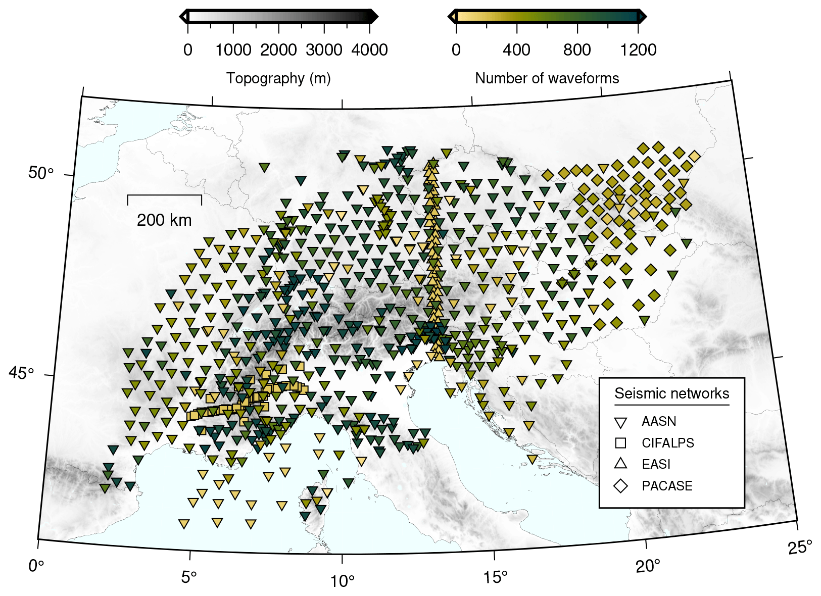
Figure 1Distribution of three-component broadband seismometers of the AlpArray Seismic Network (AASN), the China–Italy–France Alps seismic transect (CIFALPS), the Eastern Alpine Seismic Investigation (EASI), and the Pannonian–Carpathian–Alpine Seismic Experiment (PACASE) used in this study (Hetényi et al., 2018a, b; Zhao et al., 2016; Hetényi et al., 2019). Seismic stations from AASN including the permanent stations, CIFALPS, EASI, and PACASE are respectively shown as inverted triangles, squares, triangles, and diamonds and are colored according to the number of waveforms used (Z-N-E component triplets).
2.2 Teleseismic events
Figure 2 shows the epicenters of the 1687 teleseismic earthquakes that we use for the receiver function calculations. We selected teleseismic events with M>5.5 and epicentral distance, Δ, between 30 and 90∘. These epicentral distances and earthquake magnitude ranges were used to avoid the upper mantle triplications and regional and core phases. We exclude earthquakes with large magnitudes M>8.5 because their waveforms have long and complex source-time functions that can also be contaminated with signals from large aftershocks. In our case, this threshold only discarded one earthquake (M=8.6 earthquake that took place off the west coast of northern Sumatra in April 2012 and was recorded by the CIFALPS seismic network).
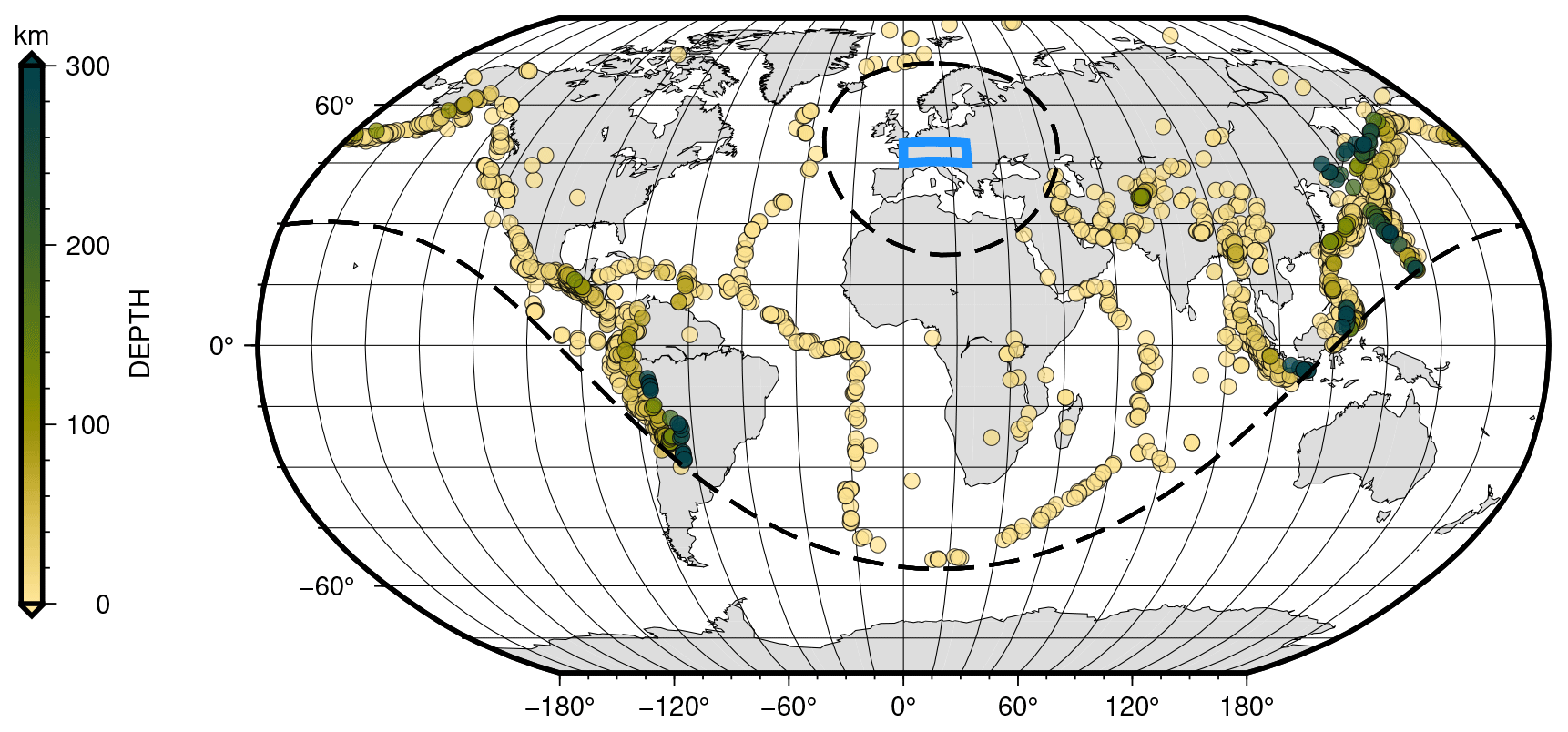
Figure 2Distribution of teleseismic events used in this study shown as circles colored according to hypocentral depths (USGS catalog; https://earthquake.usgs.gov/earthquakes, last access: October 2022). The study area is shown by the blue box. Dashed black lines show the 30 and 90∘ epicentral distance from the center of the study area.
The steps to calculate the receiver functions (RFs) and to perform the time-to-depth RF migration are summarized in the processing workflow shown in Fig. 3 and described in more detail below. The codes used for this analysis are open access (see the Code availability section for details).
3.1 Receiver function calculations
We first cut continuous seismic waveform data around the theoretical P-wave arrival times (120 s before and after) of the teleseismic events (1687 events in total) from all available seismic stations. We downsample the cut waveforms to 20 samples per second. We discard any incomplete trace or any incomplete Z-N-E triplet. This provides us with 521 762 Z-N-E waveform triplets in total.
We then rotate the horizontal components into true N and E components based on the alignment stated in the station metadata (i.e., azimuth and dip values of each channel stored in the inventory file). This step is particularly crucial for the randomly oriented horizontal components of free-fall ocean bottom seismometers of the AlpArray Seismic Network in the Ligurian Sea.
Following Hetényi et al. (2018b), we apply a first quality-control (QC) step that will help us remove anomalous traces. Particularly, this step includes the calculation of two signal-to-noise parameters: (1) the ratio between peak amplitude to background noise amplitude, and (2) the ratio between peak amplitude and background noise root mean square (rms). We also calculate the rms value of all the available seismic traces for each teleseismic event and use the median rms value for that event, median(rms). Then we discard any trace with an rms that does not meet the following criteria for that event:
where c1 and c2 are sensitivity parameters and equal to 10 and 0.1, respectively. The c1 and c2 values are based on empirically defined values (for more details, see Hetényi, 2007). This quality control ensures that we discard noisy waveforms or waveforms that contain biases introduced by local noise or problems with the seismometers. We apply this quality-control step to all three (Z-N-E) component seismograms separately.
The horizontal seismogram components are then rotated to the radial (R) and transverse (T) components, using the theoretical back-azimuth value, ϕ. This step helps to isolate the energy from the direct P wave and the converted S waves.
At this stage, we apply a second quality-control step to ensure that we keep traces with strong signals (i.e., large amplitudes). To do this, we use an algorithm based on observing changes in the amplitudes of the seismic traces within two moving time windows (i.e., ratio of short-term average, STA, to long-term average, LTA, algorithm; Allen, 1978) that is most commonly used in earthquake detection applications (e.g., Michailos et al., 2019, 2021). We apply a low-pass filter of 1 Hz to the radial component waveforms and use STA and LTA values of 3 and 50 s, respectively. We keep the waveform traces that have STA LTA ratio values larger than 2.5 and discard traces with weak signals.
Prior to the deconvolution, we (1) trim the 240 s long radial and vertical component traces 40 s before and 60 s after the P arrival, (2) remove the mean, and (3) taper the traces using a 15 s Hann window at both ends to avoid filter artifacts. We then apply a second-order 0.05–1 Hz Butterworth bandpass filter that eliminates the noisiest frequencies.
We use the iterative time-domain deconvolution approach of Ligorría and Ammon (1999) with 200 iterations to remove the effect of source-time functions. In this approach, spikes are added iteratively to the trial RF that is convolved with a Gaussian with a half width of 1 Hz. The convolution of the series of Gaussian spikes with the vertical component approximates the radial component. The predicted final radial components have high cross-correlation values (RF fit values; see Figs. A1 and A2) when compared to the observed radial traces. We chose the approach of Ligorría and Ammon (1999) among other available approaches (e.g., Gurrola et al., 1994, 1995; Park and Levin, 2000; Helffrich, 2006) based on its stability (see discussion in Lombardi et al., 2008). It should also be noted, however, that for high-quality datasets, most deconvolution methods work well, and the advantages of one method over another are insignificant (e.g., Ligorría and Ammon, 1999).
We then apply the last quality control to the calculated RFs, similar to Hetényi et al. (2015), Singer (2017), Hetényi et al. (2018b), Scarponi et al. (2021), that is based on the signal-to-noise ratio and the amplitude of the direct wave signal. For the first part of this quality control, we calculate (1) the rms of the noise from 30 to 10 s before the P-wave arrival (rmsnoi), and (2) the rms of the signal between 2 and 30 s after the P arrival (rmssig). We keep the RFs that meet the following criteria:
In addition, we require that (1) the timing of the maximum amplitude peak should be between 0 and 2 s and that (2) its amplitude should be positive and have a value between 0.05 to 0.8. The first criterion ensures that the dominant arrival is either the direct wave, expected to appear at t=0 s in Z-R RF, or the conversion at the sediment–basement interface. The second requirement on the amplitude value also helps to discard seismic traces with incorrect gain values or deconvolution artifacts (e.g., Hetényi, 2007). We discard RF traces with overly large rms values (threshold equal to 0.07; Fig. A3) which represent the top ∼2 % the traces. The results are not sensitive to the choice of this threshold; however, the chosen value enables us to discard the noisiest RF traces that are expected to mostly affect and contaminate our final migrated images.
As the last check, we visually inspected the RF traces (radial components) plotted versus their back azimuths from each individual seismic station. This final step ensures that we identify and discard any traces with low-quality results.
Figure 3Workflow summarizing the processing steps followed for (a) the receiver function calculations and (b) for the time-to-depth migration. These steps are described in detail in Sect. 3.
3.2 Common conversion point stacking
To examine the spatial variability of crustal structures, we use the common conversion point (CCP) stacking techniques that take advantage of dense arrays of seismic stations to provide images of discontinuities in the crust and upper mantle (e.g., Yuan et al., 1997; Kosarev et al., 1999; Ryberg and Weber, 2000; Zhu, 2000).
For each seismic trace, we backtrace the ray paths for S waves, assuming the theoretical P-arrival slowness. This is equivalent to assuming that all energy in the seismic trace has resulted from direct P–S conversions at horizontal boundaries. Because the study region is characterized by very significant topography and includes stations below sea level and on mountain tops, we take into account the elevation of each seismic station. Given that our study area spans approximately 2000 km, we also take into account Earth's sphericity by implementing a new CCP stacking code in a spherical coordinate system. This way the obtained profiles and maps should represent structures closer to reality.
For the time-to-depth migration, we use EPcrust (Molinari and Morelli, 2011), a 3D P- and S-wave reference velocity model based on a selection of previous geological and geophysical studies (e.g., surface-waves velocity models, active seismic experiments, receiver functions, noise correlations, and geological assumptions), that covers the entire study region. We opt to use EPcrust instead of a global 1D model (i.e., iasp91 velocity model; Kennett and Engdahl, 1991) in order to include the local structure variations within the study area. In regions with thick sedimentary layers, such as the Pannonian Basin or Po Plain, the absence of a sedimentary layer in the iasp91 model provides phase arrival times with significant time shifts. At the same time, both higher-resolution Vp and Vs models are only locally or sub-regionally available in the Alpine region. but none of these models cover the entire study area. Therefore, we have chosen to use EPcrust instead of compiling an ad hoc composite velocity model from various locally available models to ensure internally consistent results.
The grid spacing of EPcrust is 0.5∘ in latitude and longitude and consists of three layers in depth (i.e., sedimentary, upper crust, and lower crust). We use a linear interpolation method that allows us to estimate P- and S-wave velocities at any given point within the velocity model. For the depths below the EPcrust Moho, we use the velocity values of the lower crust in order to avoid mismigration with mantle velocities when the observed Moho conversion phase is later than expected from EPcrust. Conversions from below the Moho will be mismigrated, which in the context of this study focusing on Moho depth, is not of concern. We then define a 3D spherical migration grid spaced 0.05∘ in latitude and longitude and at 0.5 km in depth. Within this grid, we calculate the theoretical ray paths with a smaller, 0.25 km increment, taking into account the station elevation information. The P- and S-wave velocities along the ray paths are sampled from the interpolated EPcrust velocity model. We back-project the converted wave amplitudes of the receiver functions along these theoretical ray paths and stack them within the defined 3D spherical migration grid. This 3D grid of stacked RF amplitudes, therefore, highlights any increase or decrease in seismic velocity with depth, which primarily represents structures associated with sharp velocity changes such as the Moho interface.
4.1 Receiver functions
We obtain 112 205 quality-controlled RFs in total. Figure 4 depicts the number of RFs at each seismic station. As a general rule, we expect that there will be more RFs at stations that have longer operational times or have high-quality waveforms (e.g., stations located on bedrock). Consequently, seismic stations in southern France, the Po Basin, the Pannonian Basin, the OBS deployment in the Ligurian Sea, and the CIFALPS and EASI deployments have relatively low numbers of RFs compared to other stations because of shorter deployment times, the presence of sedimentary strata, which cause higher noise levels on the horizontal components, and because of high noise levels on the horizontal components of OBS. Furthermore, reverberations within the sedimentary layer or the water layer for OBS can obscure the Moho phase and make the RF difficult to interpret.
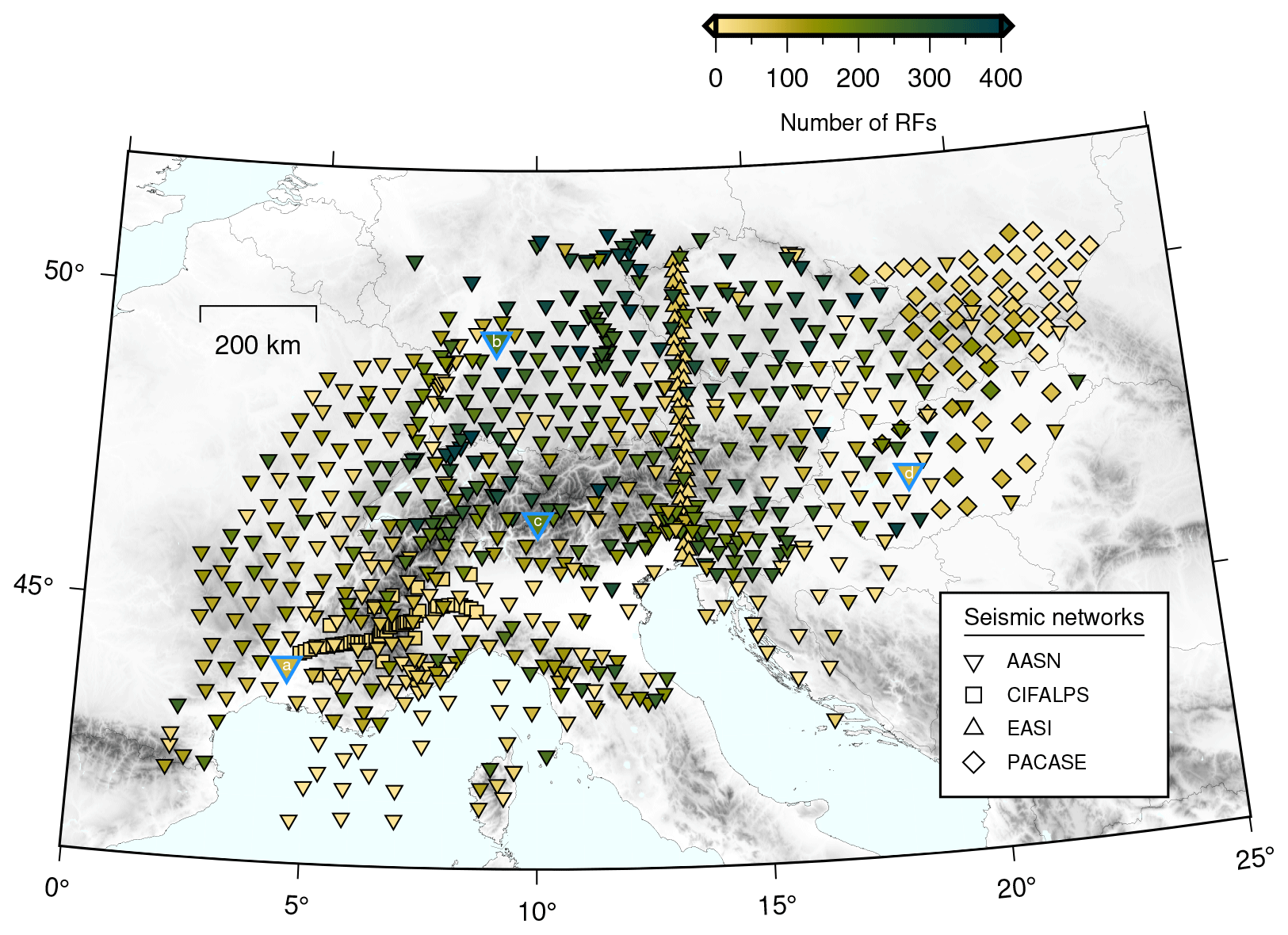
Figure 4Map showing the number of receiver functions calculated for each seismic station. Seismic stations from AASN including the permanent stations, CIFALPS, EASI, and PACASE are respectively shown as inverted triangles, squares, triangles, and diamonds and are colored according to the number of receiver functions available (see color scale). The seismic stations with blue edges marked with a, b, c, and d indicate the four stations from which we plot the receiver function stacks in Fig. 5.
We plot the calculated RFs as a function of their back-azimuth values for each station (see examples in Fig. 5) to observe any differential times, amplitudes, and polarities of the phases that may contain additional information on the inclination of the discontinuities (e.g., Cassidy, 1992). This kind of graph also helps in providing an indication of the quality of the dataset (i.e., how easily identifiable is the Ps-Moho phase, what is the total back-azimuthal coverage, how does the variation of the sharpness of the Ps-Moho phase for different back azimuths look, and is there a dipping Moho interface). Systematic variations of the timing and amplitude can indicate the presence of dipping boundaries, 360∘ periodicity, or the effect of anisotropy, and 180∘ periodicity for horizontal anisotropy (e.g., Cassidy, 1992; Levin and Park, 1997; Savage et al., 2007).
In Fig. 5, we show RFs at four different seismic stations that are located in different geologic environments in the broader European Alpine region (i.e., foreland/Molasse basin, the high Alpine region, and the Pannonian Basin) and that have a varying number of RFs due to their respective operational times during the AASN deployment. The back-azimuthal coverage is generally continuous with some gaps for the southerly and westerly directions. The amplitude of the direct P-wave is variable, presumably due to changes in the angle of incidence (i.e., epicentral distances) correlated with back azimuth. We observe sharp P and Ps-Moho phases for all seismic stations at around 0–2 and 2.5–4 s, respectively. For seismic stations located in regions with thick sedimentary layers (e.g., Pannonian Basin; Fig. 5d), these phase arrivals appear with a ca. 1–1.5 s of delay in time, similar to what Kalmár et al. (2019) observed. The delay of the initial P phase is caused by interference with the conversion at the sediment–basement interface, while the delay of the Moho phase should simply be a travel time effect, which can be corrected by a velocity model including sedimentary layer information. Seismic stations with relatively fewer RF traces (Fig. 5a) nevertheless have clear high-quality signals of comparable quality to those with longer operational times (Fig. 5b and c).
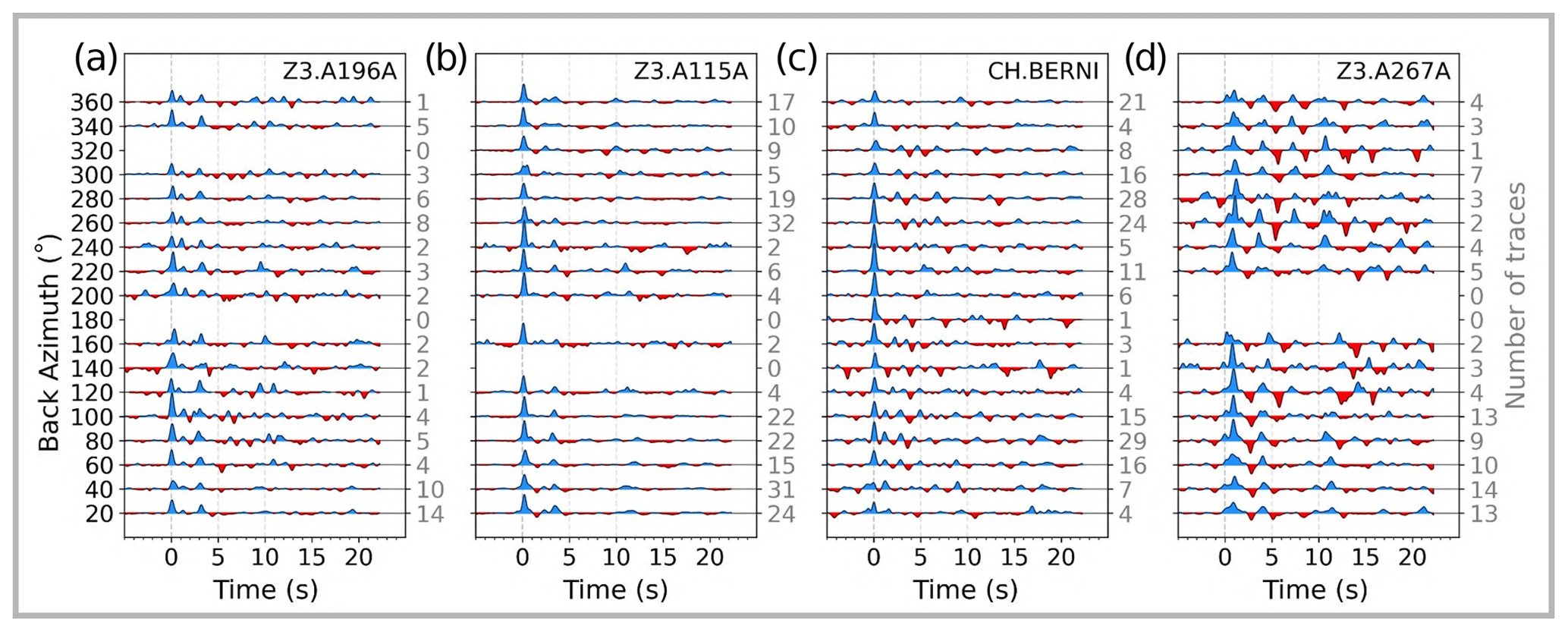
Figure 5Receiver function stacks from selected seismic stations plotted versus back azimuth. We apply a normal moveout correction and stack the traces in 20∘ wide back-azimuth bins. The number of traces contributing to each stack is shown on the right side of each panel. Dashed vertical lines indicate time delays at 0, 5, and 10 s from the P wave arrival time. Panels (a) and (b) show the RFs from two seismic stations Z3.A196A and Z3.A115A in the European foreland/Molasse Basin region. Panel (c) depicts the RFs from station CH.BERNI in the high Alpine region, and panel (d) shows station Z3.A267A in the Pannonian Basin.
4.2 Receiver function migration
To assess the coverage, we compare the station spacing with the horizontal offset of the piercing points. The lateral offset between the station location and the piercing points at the Moho is roughly half the Moho depth. Hence for a Moho ranging from ca. 22–25 km depth (beneath the Pannonian Basin) to ca. 55–60 km (beneath the Alps), the corresponding range of horizontal offsets of the piercing points is about 11–30 km. Since the nominal station spacing is 50 km, over most of the network the piercing points of neighboring stations are not significantly overlapping. We calculate the piercing points, using the EPcrust velocity model, at 35 km depth as a compromise between areas of expected shallower and deeper Moho depths (Fig. 6). The piercing points are well distributed and do not leave major gaps in coverage – with the exception of some seismic stations in the Po Basin, in the Pannonian Basin, and the OBS stations in the Ligurian Sea where the coverage is less dense due to either short operational times or the strong-quality criteria applied.
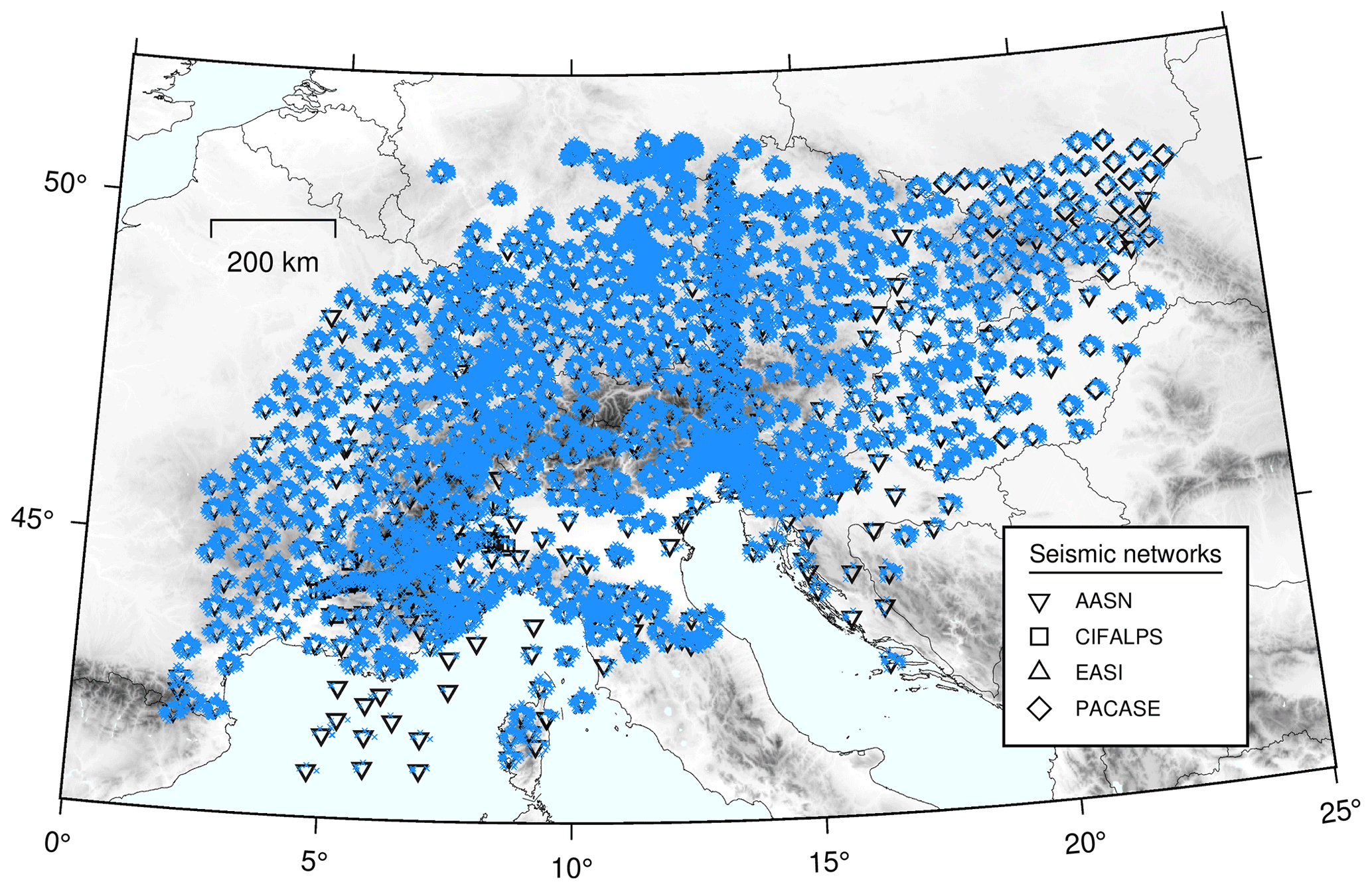
Figure 6Map depicting the piercing points (blue crosses) at 35 km depth computed for each seismic station (inverted triangles) using the EPcrust velocity model (Molinari and Morelli, 2011). The size of the crosses is based upon a Fresnel volume estimate of ∼9 km for a typical frequency of 1 Hz.
Having calculated a 3D grid of stacked migrated RF amplitudes, we are able to extract 2D migrated receiver-function cross-sections at any location within our study region. Figure 7 shows the crustal structure along three cross-sections. Namely, cross-section (A–A′) is located beneath the western Alps collocated with the CIFALPS deployment to benefit from high station density, cross-section (B–B′) beneath the central Alps, and cross-section (C–C′) beneath the Pannonian Basin and the eastern Alps. In cross-section A–A′, we observe strong migrated amplitude signals from the European Moho, which dips gently to the east–northeast. The European Moho (EU in Fig. 7) starts from depths of approximately 30 km in the west reaching gradually depths of ca. 50–55 km. The signal then weakens at around 3–3.5∘ distance along cross-section A–A′, and for the rest of the cross-section, the Adriatic Moho (AD in Fig. 7) is generally harder to interpret. The crustal geometry in cross-section A–A′ is in good agreement with the result of Zhao et al. (2015) who used the CIFALPS seismic data and Monna et al. (2022) who jointly inverted P and S receiver functions using AASN seismic data. In cross-section B–B′, we also observe strong amplitudes for the European Moho (∼30 km in the northwest that gently dips down to ∼55 km beneath the Alps). The Adriatic Moho is a bit easier to identify, with respect to cross-section A–A′, with depths of around 30 km (around 4∘ in B–B′). Farther southeast, the B–B′ profile continues through the Po Basin (PB in Fig. 7) where the signal is harder to interpret, as the Moho no longer appears as a continuous interface; possibly this is caused by interference from multiples of the sediment–basement interface, but also there are fewer high-quality RFs available for this area. Finally cross-section C–C′ starts from the Po Basin where again no clear continuous interface is visible; the whole section is harder to interpret than previous ones, especially beneath the eastern Alps. The Adriatic Moho at offsets 1–3∘ is between 35 and 40 km deep. Farther northeast, the European Moho lies between 25 and 30 km depth beneath the Vienna Basin and past the western Carpathians (VB and WC in Fig. 7).

Figure 7Migrated receiver-function cross-sections in spherical coordinates along lines A–A′ (top panel), B–B′ (middle panel), and C–C′ (lower panel) as marked in the inset map. Note that cross-section D–D′ is shown in Fig. 9. White and gray diamonds represent the manually determined certain and uncertain Moho picks, respectively. For comparison, the solid black and dashed black lines depict the Moho depths calculated by Grad and Tiira (2009) and Spada et al. (2013), respectively. EU: European Moho, AD: Adriatic Moho, PB: Po Basin, VB: Vienna Basin, and WC: West Carpathians. All cross-sections are smoothed and filtered and have no vertical exaggeration, profile curvature represents real Earth sphericity. The inset map shows the location of seismic stations used with inverted blue triangles. Solid lines indicate the cross-section locations with tracks every 1∘ distance.
4.3 Moho depth map
To compile the new Moho depth map, we manually pick Moho depths on 21 equally spaced cross-sections along the meridians (3–23∘) and another 10 equally intercepting cross-sections along the parallels (43–50∘). Refer to the Supplement for all cross-sections and manually defined picks. We determine the Moho depth picks based on the strength and continuity of the amplitude signal. We assign the picks on the maximum of the signal. In cases where the signal appears to be unclear (weaker signal) or not completely continuous, we assign uncertain Moho depth picks. For examples where the signal is double (overlapping Moho discontinuities), we choose to pick the shallower signal. Double signals might be associated with underthrusted lower crustal slivers or subduction (e.g., Spada et al., 2013; Hetényi et al., 2018b; Mroczek et al., 2023); therefore picking the shallower Moho ensures the bottom of a continuous crustal stack is picked.
This analysis provides us with a dense grid of Moho depths in the broader European Alpine region (Fig. 8a). We interpolate the Moho depth points using a linear interpolation method to obtain a continuous image of the Moho depth distribution (Fig. 8b). We also test interpolating (1) the Moho depth picks separately for each plate (i.e., European, Adriatic, and Ligurian) and (2) using only the certain Moho depth picks (excluding uncertain) and obtained very similar patterns (Figs. A4 and A5). The plate boundaries are taken from Spada et al. (2013)'s Moho map, although in some locations our migrated RF profiles point to slightly different plate limit positions. Moho depths vary from ∼30 to ∼60 km in the broader European Alpine region, with the deepest values (>50 km) observed near the highest topography of the Alps close to the plate boundary between the European and Adriatic plates. The majority of the European plate has Moho depths of around 30 km, which is typical for the continental crust in western Europe. We are able to estimate very few Moho depth picks in the Ligurian Sea and no picks in the Adriatic Sea due to the lack of deployed stations.
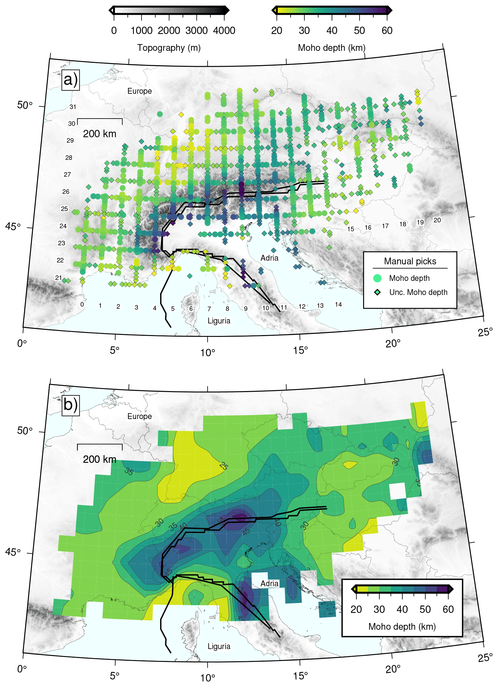
Figure 8(a) Map showing the spatial variations of Moho depths for the broader European Alpine region. Circles and diamonds with black edges depict certain and uncertain manually picked Moho depths, respectively. Numbers indicate the names of the cross-sections that are used for making the Moho picks (see manually determined Moho picks for each cross-section in the Supplement). Thick black lines depict the plate boundaries between the European, Adriatic, and Ligurian plates adapted from Spada et al. (2013). (b) Contoured distribution of all Moho depths. Empty boxes depict regions where the interpolation method did not provide any results.
We present new RF migrated profiles and a new Moho depth map uniformly derived for the broader European Alpine region, based on receiver functions and time-to-depth migration calculations of seismic waveform data from four temporary seismic networks (i.e., AASN, EASI, CIFALPS, and PACASE) and permanent stations. Starting from continuous data, we apply a series of systematic processing steps (see Fig. 3) and calculate an unprecedented number of high-quality RFs that allow us to image the variations of Moho depth in the Alpine region and its forelands in great detail.
5.1 Comparison with previous Moho depth models
Our Moho depth estimates and migrated images are comparable with and generally supported by the results from previous studies in the region (e.g., Grad and Tiira, 2009; Spada et al., 2013), with some differences which we attribute to a more complete spatial data coverage and the different approaches used. In general, our Moho estimates are relatively shallower in the European plate and relatively deeper in the Adria plate when compared to the two previous studies (Fig. A6; Grad and Tiira, 2009; Spada et al., 2013). The main differences are located along the tectonic plate boundaries, especially along the Ivrea-Verbano zone where estimates around the protruding Ivrea geophysical body cause large differences. This is mostly due to differences in the coverage of seismic stations and the respective method of interpolation. Denser arrays can provide a higher local resolution for the Moho (e.g., 5 km spacing of IvreaArray; Scarponi et al., 2021). When all quantified Moho depth differences are considered (Fig. A7), our Moho depth estimates are on average 0.6 km deeper than those of Spada et al. (2013) and 0.4 km shallower than those of Grad and Tiira (2009). The standard deviation of the difference distribution – which includes the high values mentioned above – is respectively 7.6 and 6.4 km.
In profile A–A′ of Fig. 7, our deepening Moho signal and picks of the European plate can be followed to 3.25∘ distance at least, while that of Grad and Tiira (2009) starts transitioning to a shallower depth at 2.75∘ distance (∼50 km to the west), and that of Spada et al. (2013) features a sharper jump at around 3.1∘ distance. On the Adria side, the Moho depth estimates of the three models differ, which is expected given the complexity related to the shallow intruding Ivrea geophysical body that requires more detailed analyses (e.g., Scarponi et al., 2021). In profile B–B′, the situation at the Europe–Adria limit is somewhat similar to that in profile A–A′. Our European Moho signal and picks can be tracked until 3.7∘ distance, while Grad and Tiira (2009)'s estimates become shallower already at 3∘ distance (70 km to the NW), and Spada et al. (2013)'s jump is at 3.5∘ distance. The continuity of the European Moho signal beneath Adria in both profiles in our images could be explained by the teleseismic waves imaging this zone from below, while a good portion of Spada et al. (2013)'s dataset is from active seismic imaging from above, hence determining the shallower discontinuity. In that sense, defining the boundary between two plates in a collision zone goes beyond the task of tracing a line on a map, and it requires 3D analysis and the representation of overlapping Mohos, something that was done by Spada et al. (2013) in some regions. From a geodynamic perspective, this is not surprising, as during collisional processes, different layers of the lithosphere decouple from each other, may deform independently from each other, and also imbricate between plates. In profile C–C′, the three Moho models show fewer differences, estimated at ∼5 km and locally at 10 km in depth. The largest difference at around 4∘ distance reveals a shallower Moho in our model compared to Grad and Tiira (2009), which could reflect a thinner crust in the transition zone of the easternmost Alps to the Pannonian Basin.
5.2 Comparison of RF migrated profiles using different velocity models
To examine the influence of the laterally heterogeneous velocity model used for migration, we compare migrated profiles using two different velocity models (i.e., iasp91 and EPcrust in our case). For this comparison, we choose a cross-section along the EASI profile. By doing this, we are also able to compare our results to the previous study of Hetényi et al. (2018b). Figure 9 depicts the migrated cross-section images from north to south along the EASI seismic network using the EPcrust velocity model (top panel) and the global 1D iasp91 velocity model (lower panel). Although the overall pattern is the same, there are significant differences of more than 5 km in the absolute inferred Moho depth that are mostly due to the absence of a sedimentary layer in the iasp91 model (depths of <5 km). In addition, these images are also in good agreement with the results of Grad and Tiira (2009), Spada et al. (2013), and Hetényi et al. (2018b) to the first order. A notable zone of difference is the root of the Alps, between 3.5 and 4∘ distance (Fig. 9), where Hetényi et al. (2018b) interpreted the Moho as the bottom of a broad velocity gradient, while the two other models relied mostly on active seismic data and interpreted the top of that zone. Further discussion would require more detailed processing, such as RF multiples, initiated in Hetényi et al. (2018b) and continued in Mroczek and Tilmann (2021).

Figure 9Comparison between migrated receiver-function cross-sections along the EASI seismic network (cross-section D–D′ in Fig. 7) calculated using the EPcrust velocity model (top panel) and iasp91 velocity model (lower panel). The solid, dashed, and dotted lines show the Moho depths estimated by Grad and Tiira (2009) that is a compilation of Moho depths, Spada et al. (2013) who used a modified iasp91 velocity model for the migration calculations, and Hetényi et al. (2018b) who utilized EPcrust for migration, respectively. Stripes between the panels highlight the location of the orogenic root, where Hetényi et al. (2018b) interpreted the Moho at the bottom of a broad velocity-gradient imaged by teleseismic waves from below (represented by dots), while other studies (e.g., Spada et al., 2013) interpreted the Moho using controlled-source waves reflecting from the top of this gradient.
5.3 Limitations
The semi-automatic workflow used here includes strict quality criteria that discard almost of the available seismic waveforms. This order of magnitude of discarded waveforms is comparable to other receiver-function studies (e.g., Hetényi et al., 2018b; Scarponi et al., 2021; Kalmár et al., 2021). However, by using these strict quality criteria, (1) we ensure that our final results are less likely to be contaminated by low-quality RFs traces, and (2) we are able to automatically process a large number of seismic waveforms and simplify manual inspections that would be extremely time-consuming. We note that these quality-control criteria and the frequency band used are tuned for identifying crustal structures and that other applications of RFs may require adjusted selections.
Despite the high density of seismic waveform data available, we emphasize that our Moho depth estimates have limitations and uncertainties that are inherently difficult to assess. For example, the Moho depth estimates can contain errors associated (1) with the quality and consistency of the manual Moho picks and (2) with the inherited uncertainties from the EPcrust velocity model used for migration (e.g., see differences in Moho depths in Fig. 9). Furthermore, we have solely focused on direct Ps conversions and have not investigated either multiples or illumination directions for effects of dip or anisotropy (e.g., Bianchi and Bokelmann, 2014; Bianchi et al., 2021). Ultimately, a major source of depth uncertainty is the 3D variability of the real seismic wave speed structure with respect to the three-layer, 0.5∘ distance resolution EPcrust model. This and lower success in the RF quality control makes picks and interpretations particularly vulnerable in areas of sedimentary basins, and we would recommend closer (re)analyses for studies focusing on those areas. Extending the analysis by including the crustal multiples (e.g., PpSs, PpPs) is a potential future direction that would allow an estimate of Moho depth without assuming a fixed ratio over local to regional scales. For fully 3D Vs structure inversion based on RFs, we refer to Colavitti and Hetényi (2022).
Continuous seismic data from the seismic networks used in this study can be found at the European Integrated Data Archive (EIDA; http://www.orfeus-eu.org/data/eida/; EIDA, 2022) with the following network codes: Z3 (AlpArray Seismic Network: AlpArray Seismic Network, 2015, https://doi.org/10.12686/ALPARRAY/Z3_2015); XT (EASI: AlpArray Seismic Network, 2014, https://doi.org/10.12686/alparray/xt_2014), BW (BayernNetz Department of Earth and Environmental Sciences Geophysical Observatory University of Munchen, 2001, https://doi.org/10.7914/SN/BW); CH (Swiss Seismological Service, SED, 1983, https://doi.org/10.12686/SED/NETWORKS/CH), GR (German Regional Seismic Network (GRSN): Federal Institute for Geosciences and Natural Resources BGR, 1976, https://doi.org/10.25928/mbx6-hr74), IV (Istituto Nazionale di Geofisica e Vulcanologia, INGV, 2005, https://doi.org/10.13127/SD/X0FXNH7QFY), MN (the Mediterranean Network: MedNet Project Partner Institutions, 1990, https://doi.org/10.13127/SD/fBBBtDtd6q); NI (North-East Italy Broadband Network: OGS, Istituto Nazionale di Oceanografia e di Geofisica Sperimentale and University of Trieste, 2002, https://doi.org/10.7914/SN/NI), OE (Austrian Seismic Network: ZAMG – Zentralanstalt für Meterologie und Geodynamik, 1987, https://doi.org/10.7914/SN/OE), OX (North-East Italy Seismic Network: Istituto Nazionale di Oceanografia e di Geofisica Sperimentale – OGS, 2016, https://doi.org/10.7914/SN/OX), FR (RESIF and other broadband and accelerometric permanent networks in metropolitan France: RESIF, 1995, https://doi.org/10.15778/RESIF.FR), SI (Province Südtirol: https://www.fdsn.org/networks/detail/SI/; International Federation of Digital Seismograph Networks, 2022), SL (Seismic Network of the Republic of Slovenia: Slovenian Environment Agency, 1990, https://doi.org/10.7914/SN/SL), ST (Trentino Seismic Network: Geological Survey-Provincia Autonoma di Trento, 1981, https://doi.org/10.7914/SN/ST), and YP (CIFALPS: Zhao et al., 2016, https://doi.org/10.15778/RESIF.YP2012). PACASE data are archived at the EIDA node at LMU with the network code ZJ (Hetényi et al., 2019, https://doi.org/10.7914/SN/ZJ_2019) and are embargoed until 30 June 2025.
The following datasets are freely available in a Zenodo repository with the following DOI: https://doi.org/10.5281/zenodo.7695125 (Michailos et al., 2023). Firstly, we include all the downloaded seismic waveform data (ZNE components; 120 s before and after the theoretical P-wave arrival) prior to RF calculation apart from those from the PACASE seismic network that are under embargo. Secondly, we include the receiver functions calculated here (both radial and transverse components). The repository also contains the plots, in PNG format, of the stacked receiver functions from all the seismic stations used here. Finally, we also include (1) the Moho depth picks information shown in the main article's Fig. 8a, (2) details of the teleseismic earthquakes, and (3) a list of all the seismic stations we use in three separate CSV format files.
All codes used for this work are actively developed on GitHub at the following repository: https://github.com/kemichai/rfmpy (last access: May 2023) and https://doi.org/10.5281/zenodo.7937575 (Michailos, 2023). A tutorial for calculating RFs and time-to-depth migration for a subset of the data used is also available on the following website: https://rfmpy.readthedocs.io/en/latest/tutorial.html (last access: May 2023). The codes developed here are mostly based on open-source software like ObsPy (Beyreuther et al., 2010; Krischer et al., 2015) and EQcorrscan (Chamberlain et al., 2018). We use GMT (Wessel et al., 2019) for creating maps, Matplotlib (Hunter, 2007) for graphs, and the Scientific Color Maps (Crameri, 2021) for color scales.
We start from continuous seismic waveform data that cover the broader European Alps region, calculate RFs and perform 3D time-to-depth migration calculations in a spherical coordinate system. In particular, we calculate 112 205 RFs in total at 708 different seismic stations. The RF traces are freely available (see the Data availability section for details). We also compile a new homogeneously derived Moho depth map of the broader European Alps.
We have developed codes in Python for RF calculations and CCP stacking in spherical coordinates that are open-access, documented, and tested on GitHub. The codes are actively developed, and we welcome any code improvements or suggestions and error reports from the community. A tutorial for calculating RFs and time-to-depth migrations for a subset of our data is also available (see Code availability section).
We anticipate that this high-quality and homogeneously calculated RF dataset, along with the new Moho depth map of the European Alps, can provide helpful information for interdisciplinary imaging and modeling studies investigating the geodynamics of the European Alps orogen and its forelands (e.g., joint inversions with other datasets).
This appendix contains seven supporting figures that are referred to in the main paper.
Figure A1 depicts the spatial distribution of the cross-correlation, cc, values between predicted and observed radial waveforms at the 708 different seismic stations used here.
Figure A2 illustrates these cc values as a function of epicentral distance, event magnitude, and depth.
Figure A3a shows the sorted RMS values of each individual RF trace calculated here along with the threshold we set to discard noisy RFs.
Figure A3b presents the seismic stations from which the RF traces were discarded.
Figures A4 and A5 show two separate tests that we use to ensure that the interpolating method used gives stable results. Figure A4 presents the contoured distribution of the Moho depths for each plate separately (i.e., European, Adriatic, and Ligurian) in map view. Figure A5 depicts the contoured distribution of the Moho depths only using certain Moho depth picks (excluding uncertain ones) in map view.
Finally, Figs. A6 and A7 provide a quantitative comparison of our Moho depth estimates with those from previous studies.
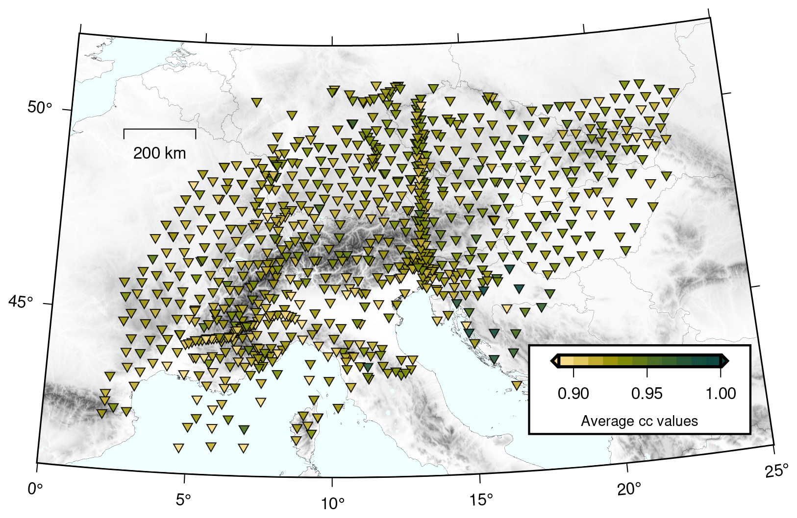
Figure A1Spatial distribution of average RF fit values (i.e., cross-correlation, cc, value between predicted and observed RF spikes) on each seismic station. Seismic stations are depicted as inverted triangles and colored according to their cc values (see color scale).

Figure A2RF fit values (cross-correlation values between predicted and observed RF spikes) versus the event-receiver distance (degrees), the earthquake's magnitude, and the earthquake's hypocentral depth (km).

Figure A3(a) Distribution of sorted RMS values calculated on each individual RF trace. The horizontal red continuous line indicates the threshold chosen above which we discard RFs (2472 in total) and exclude them from the time-to-depth migration calculations. (b) Map showing the distribution of the RFs that we exclude from the time-to-depth migration calculations. The triangles are colored according to the number of RFs discarded as a percentage of all the RFs calculated for each seismic station. Seismic stations with no RFs removed are depicted as inverted white triangles.

Figure A4Contoured distribution of Moho depths separated for each plate (i.e., European, Adriatic, and Ligurian). Empty boxes depict regions where the interpolation method did not provide any results.
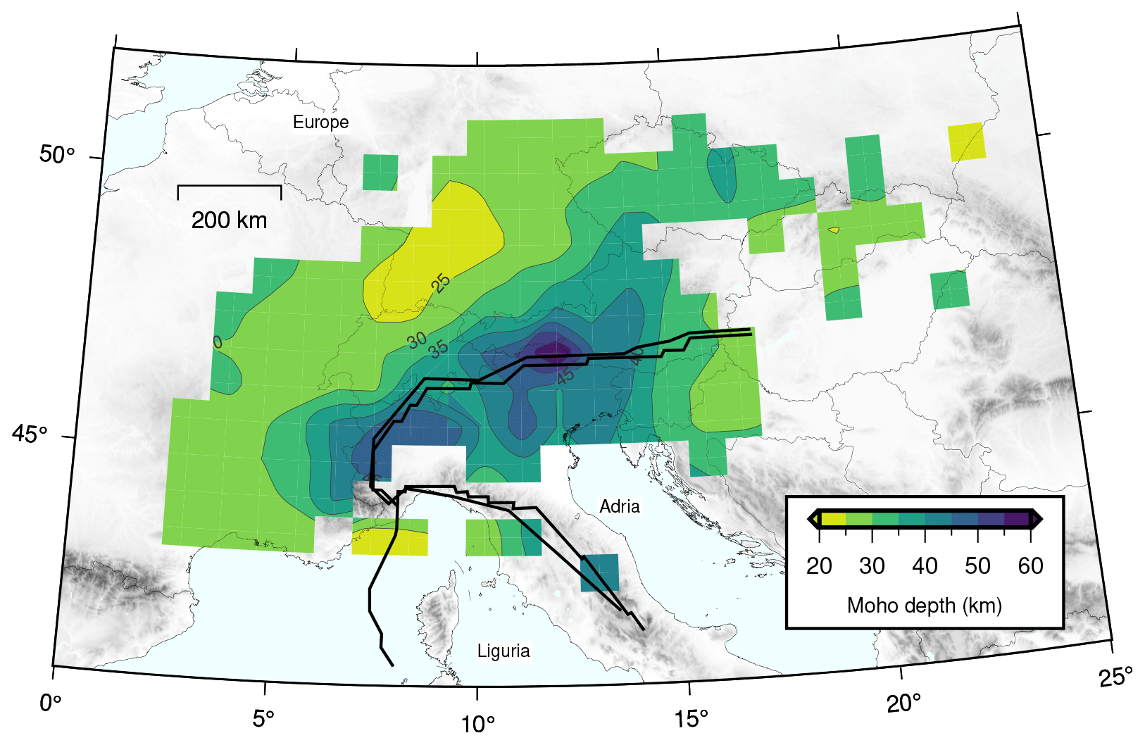
Figure A5Contoured distribution of certain Moho depth picks (excluding uncertain picks). Empty boxes depict regions where the interpolation method did not provide any results.
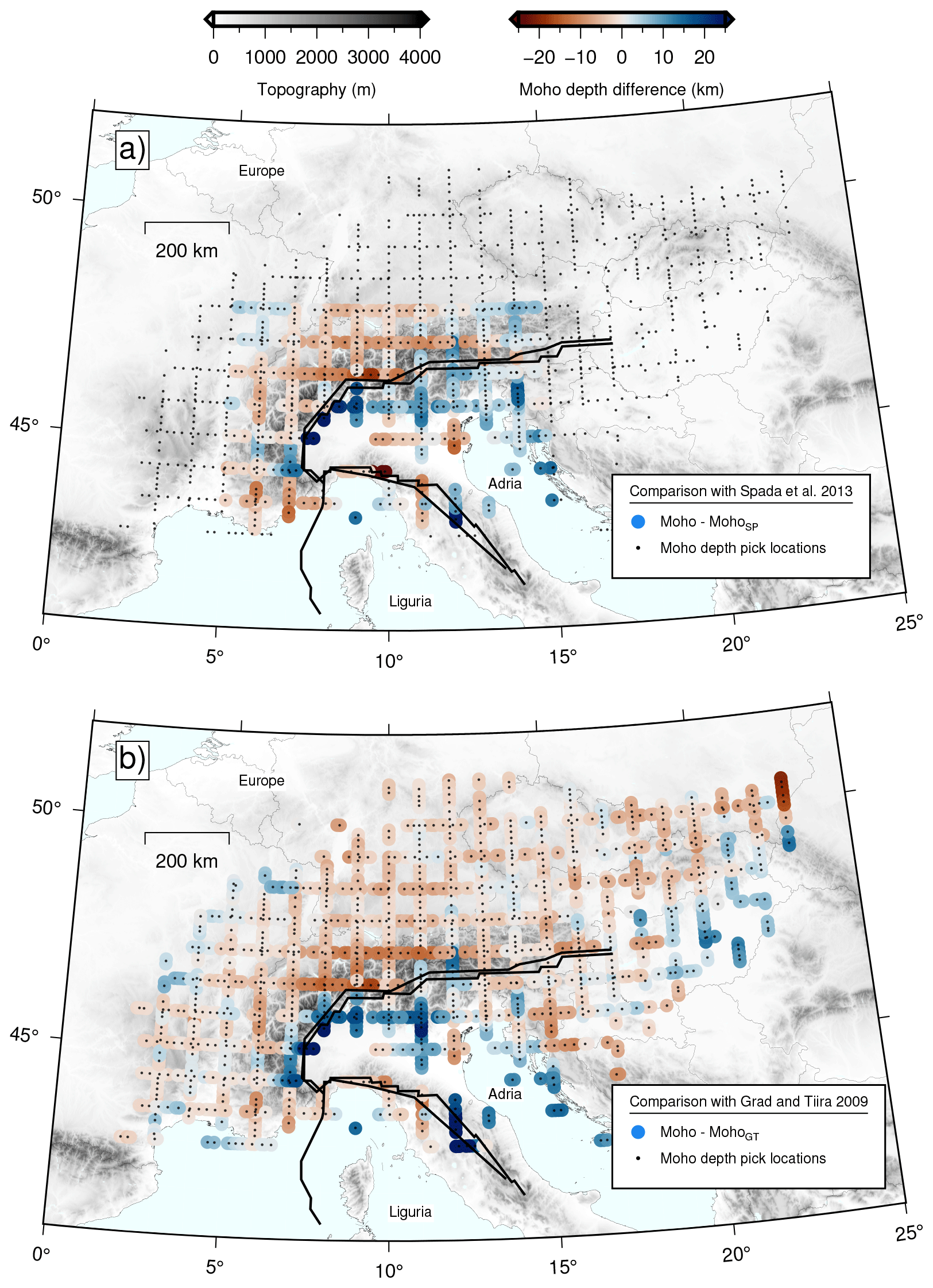
Figure A6Maps showing the spatial distribution of the differences in Moho depth estimates between our estimates, the locations of which are shown as black dots, and those of (a) Spada et al. (2013) and (b) Grad and Tiira (2009).
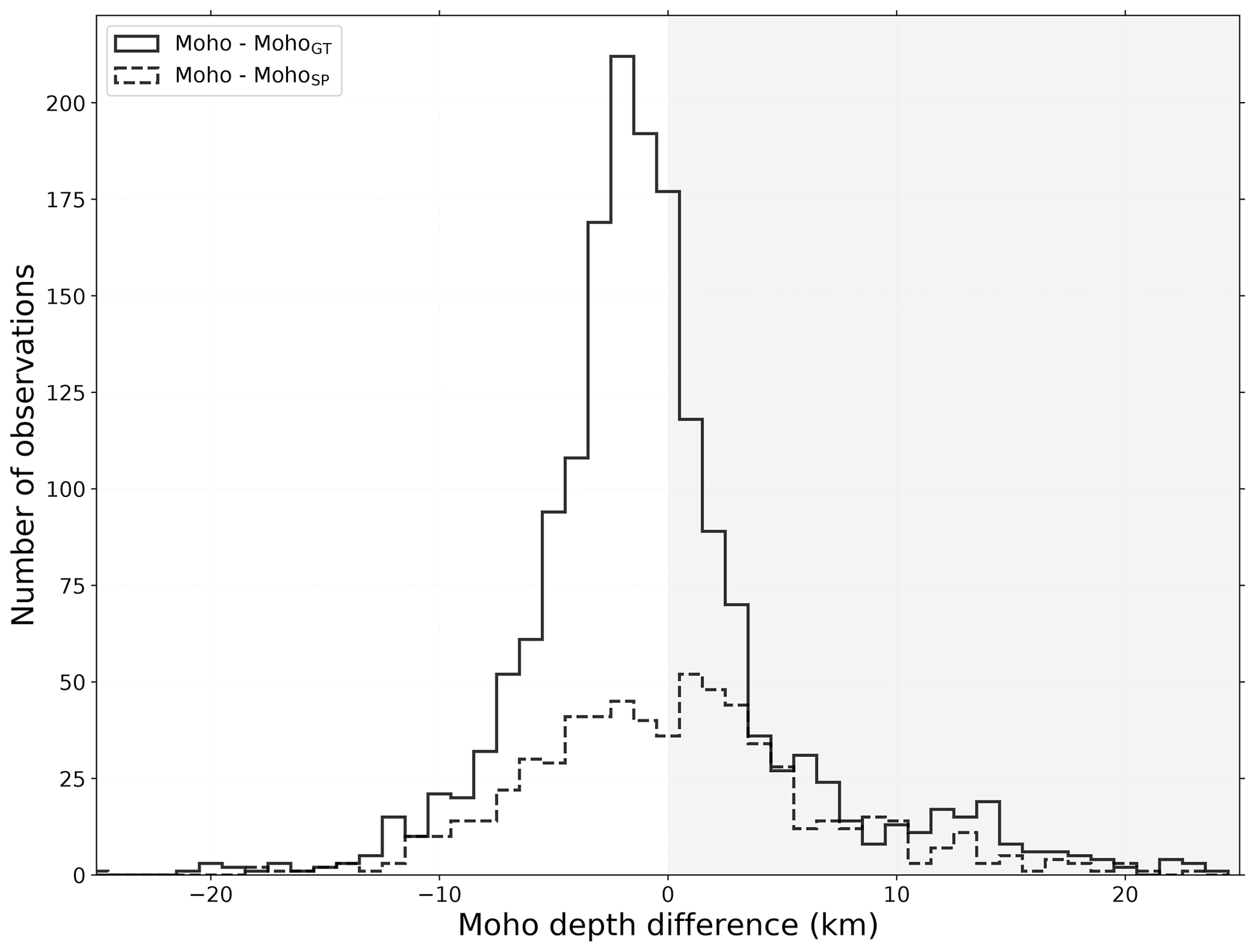
Figure A7Histogram depicting the difference between our Moho depth estimates and those of Spada et al. (2013) and of Grad and Tiira (2009). The gray-shaded background highlights the measurements for which our Moho estimates are relatively deeper than those of the two previous studies. The average value of the difference between our Moho depth estimates and those of Spada et al. (2013) is 0.6±7.6 km (median = 0.2 km) and km (median km) with those of Grad and Tiira (2009).
The supplement related to this article is available online at: https://doi.org/10.5194/essd-15-2117-2023-supplement.
The AlpArray-PACASE team: Yongki Aiman, Götz Bokelmann, Clément Estève, Erik Grafendorfer, Richard Kramer, Yang Lu (Department of Meteorology and Geophysics, University of Vienna, Vienna, Austria), Hana Kampfová-Exnerová, Peter Kolinsky, Jiri Kvapil, Cédric Legendre, Luděk Vecsey, Helena Žlebčíková (Institute of Geophysics, Czech Academy of Sciences, Prague, Czech Republic), Jörg Ebbing, Amr El-Sharkawy, Thomas Meier, Janina Stampa (Christian Albrechts Universität, Kiel, Germany), Wolfgang Friederich, Marcel Paffrath (Ruhr-University Bochum, Institute of Geology, Mineralogy and Geophysics, Bochum, Germany) Mark Handy, Emanuel Kästle (Freie Universität Berlin, Berlin, Germany), Boris Kaus (Institute of Geosciences, Johannes Gutenberg University Mainz, Mainz, Germany), Michael Korn (University Leipzig, Institute of Geophysics and Geologie, Leipzig, Germany), Andreas Rietbrock (Department of Geophysics, Karlsruhe Institute of Technology, Karlsruhe, Germany), Georg Rümpker (Institute of Geosciences, Goethe-University Frankfurt, Frankfurt, Germany), Antje Schlömer, Joachim Wassermann (Ludwig-Maximilians-Universität, München, Germany), Christine Thomas (Institute for Geophysics, University of Münster, Münster, Germany), István Bozsó, Eszter Szűcs, Bálint Süle, Viktor Wesztergom (Institute of Earth Physics and Space Science, Sopron, Hungary), Csenge Czanik, Barbara Czecze, Máté Timkó, Zoltán Wéber (Kövesligethy Radó Seismological Observatory, Institute of Earth Physics and Space Science, Budapest, Hungary), Somayeh Abdollahi (Department of Seismic Lithospheric Research, Institute of Geophysics Polish Academy of Sciences, Warszawa, Poland), Maciej Mendecki, Dariusz Nawrocki (University of Silesia in Katowice, Institute of Earth Sciences, Faculty of Natural Sciences, Poland), Miroslav Bielik, Kristian Csicsay, Lucia Fojtíková, Dominika Godová, Miriam Kristeková, Jan Vozár (Earth Science Institute, Slovak Academy of Sciences, Bratislava, Slovakia), Josef Kristek (Faculty of Mathematics, Physics, and Informatics, Comenius University in Bratislava, Bratislava, Slovakia), and Juraj Papčo (Department of Theoretical Geodesy, Faculty of Civil Engineering, Slovak University of Technology, Bratislava, Slovakia)
KM led the investigation, developed the codes, and performed the analyses. GH provided initial ideas for the research and guidance. MS also contributed to developing the codes. KM performed the visualization and wrote the original paper draft. Subsequent drafts received reviews and edits from all the co-authors. Further to this, co-authors IB, FL, FT, StM, GH, JV, AP, PŚ, JP, DK, JS, MDB, AG, FPL, and SiS have contributed in downloading different seismic waveform data used here. All authors have read and approved the final version of the paper.
The contact author has declared that none of the authors has any competing interests.
Publisher's note: Copernicus Publications remains neutral with regard to jurisdictional claims in published maps and institutional affiliations.
Konstantinos Michailos was supported by the Swiss National Science Foundation project OROG3NY on which György Hetényi was the principal investigator (grant no. PP00P2_187199). We are grateful to the operators of the permanent seismic networks that make their data available through the European Integrated Data Archive (EIDA). The authors would like to thank all members of the AlpArray Seismic Network team and the AlpArray-EASI working group and field team: Rafael Abreu, Ivo Allegretti, Maria-Theresia Apoloner, Coralie Aubert, Ludwig Auer, Sacha Barman, Maxime Berc, Simon Besançon, Didier Brunel, Marco Capello, Adriano Cavaliere, Claudio Chiarabba, Jérôme Chèze, John Clinton, Glenn Cougoulat, Wayne Crawford, Luigia Cristiano, Tibor Czifra, Stefania Danesi, Romuald Daniel, Anke Dannowski, Iva Dasović, Anne Deschamps, Jean-Xavier Dessa, Cécile Doubre, Ezio D’alema, Sven Egdorf, Laura Ermert, Tomislav Fiket, Kasper Fischer, Sigward Funke, Domenico Giardini, Pascal Graf, Katalin Gribovszki, Gidera Gröschl, Stefan Heimers, Davorka Herak, Marijan Herak, Marcus Herrmann, Stefan Hiemer, Hans Huber, Johann Huber, Dejan Jarić, Yan Jia, Peter Jordakiev, Hélène Jund, Edi Kissling, Stefan Klingen, Bernhard Klotz, Paula Koelemeijer, Heidrun Kopp, Edith Korger, Krešo Kuk, Lothar Kühne, Dietrich Lange, Jürgen Loos, Sara Lovati, Deny Malengros, Lucia Margheriti, Xavier Martin, Marco Massa, Francesco Mazzarini, Irene Molinari, Milena Moretti, Helena Munzarová, Laurent Métral, Anna Nardi, Anne Obermann, Patrick Ott, Jurij Pahor, Damiano Pesaresi, Daniel Petersen, Davide Piccinini, Thomas Plenefisch, Silvia Pondrelli, Catherine Péquegnat, Ehsan Qorbani, Roman Racine, Miriam Reiss, Meysam Rezaeifar, Joachim Ritter, Marc Régnier, Korbinian Sager, Marco Santulin, Werner Scherer, Detlef Schulte-Kortnack, Stefano Solarino, Daniele Spallarossa, Kathrin Spieker, Angelo Strollo, Gyöngyvér Szanyi, Robert Tanner, Martin Thorwart, Stefan Ueding, Massimiliano Vallocchia, René Voigt, Christian Weidle, Gauthier Weyland, Stefan Wiemer, Sacha Winterberg, Felix Wolf, David Wolyniec, Thomas Zieke, Martina Čarman, Vesna Šipka, Mladen Živčić, and Saulė Žukauskaitė. We would also like to thank the members of the AlpArray-PACASE field team: Petr Jedlicka, Josef Kotek, Luděk Vecsey, Zoltán Gráczer, Bálint Süle, Kristián Csicsay, Marianna Bognár, Florian Fuchs, Petr Kolinsky, Gerrit Hein, Artemii Novoselov, Sven Schippkus, Erik Grafendorfer, Yang Lu, Yongki Aiman, Richard Kramer, Antje Schlömer, Joachim Wassermann, Weronika Materkowska, Maciej Mendecki, Agnieszka Bracławska, and Szymon Orynski.
This research has been supported by the Swiss National Science Foundation (grant no. PP00P2_187199 “OROG3NY”); the National Research, Development, and Innovation Fund, Hungary (grant nos. K141860 and PD142953); the National Science Centre, Poland (agreement no. UMO-2019/35/B/ST10/01628); and the Grant Agency of the Czech Republic (GACR; grant no. 21-25710S).
This paper was edited by Kirsten Elger and reviewed by two anonymous referees.
Allen, R. V.: Automatic earthquake recognition and timing from single traces, B. Seismol. Soc. Am., 68, 1521–1532, 1978. a
AlpArray Seismic Network: Eastern Alpine Seismic Investigation (EASI) – AlpArray Complimentary Experiment, AlpArray Working Group. Other/Seismic Network [data set], https://doi.org/10.12686/ALPARRAY/XT_2014, 2014. a
AlpArray Seismic Network: AlpArray Seismic Network (AASN) temporary component, AlpArray Working Group. Other/Seismic Network [data set], https://doi.org/10.12686/alparray/z3_2015, 2015. a
Artemieva, I. M. and Thybo, H.: EUNAseis: A seismic model for Moho and crustal structure in Europe, Greenland, and the North Atlantic region, Tectonophysics, 609, 97–153, https://doi.org/10.1016/j.tecto.2013.08.004, 2013. a
Beyreuther, M., Barsch, R., Krischer, L., Megies, T., Behr, Y., and Wassermann, J.: ObsPy: A Python Toolbox for Seismology, Seismol. Res. Lett., 81, 530–533, https://doi.org/10.1785/gssrl.81.3.530, 2010. a
Bianchi, I. and Bokelmann, G.: Seismic signature of the Alpine indentation, evidence from the Eastern Alps, J. Geodynam., 82, 69–77, https://doi.org/10.1016/j.jog.2014.07.005, 2014. a
Bianchi, I., Ruigrok, E., Obermann, A., and Kissling, E.: Moho topography beneath the European Eastern Alps by global-phase seismic interferometry, Solid Earth, 12, 1185–1196, https://doi.org/10.5194/se-12-1185-2021, 2021. a, b
Blundell, D. J., Freeman, R., Mueller, S., and Button, S.: A continent revealed: The European Geotraverse, structure and dynamic evolution, Cambridge University Press, 1992. a
Cassidy, J. F.: Numerical experiments in broadband receiver function analysis, B. Seismol. Soc. Am., 82, 1453–1474, https://doi.org/10.1785/BSSA0820031453, 1992. a, b
Chamberlain, C. J., Hopp, C. J., Boese, C. M., Warren‐Smith, E., Chambers, D., Chu, S. X., Michailos, K., and Townend, J.: EQcorrscan: Repeating and Near‐Repeating Earthquake Detection and Analysis in Python, Seismol. Res. Lett., 89, 173–181, https://doi.org/10.1785/0220170151, 2018. a
Colavitti, L. and Hetényi, G.: A new approach to construct 3-D crustal shear-wave velocity models: method description and application to the Central Alps, Acta Geod. Geophys., 57, 529–562, https://doi.org/10.1007/s40328-022-00394-4, 2022. a, b, c
Crameri, F.: Scientific colour maps, Zenodo [data set], https://doi.org/10.5281/zenodo.5501399, 2021. a
Department of Earth and Environmental Sciences, Geophysical Observatory, University of Munchen: BayernNetz, International Federation of Digital Seismograph Networks [data set], https://doi.org/10.7914/SN/BW, 2001. a
Diehl, T., Kissling, E., Husen, S., and Aldersons, F.: Consistent phase picking for regional tomography models: Application to the greater Alpine region, Geophys. J. Int., 176, 542–554, https://doi.org/10.1111/j.1365-246X.2008.03985.x, 2009. a
Di Stefano, R., Bianchi, I., Ciaccio, M. G., Carrara, G., and Kissling, E.: Three-dimensional Moho topography in Italy: New constraints from receiver functions and controlled source seismology, Geochem. Geophys. Geosyst., 12, 1–15, https://doi.org/10.1029/2011GC003649, 2011. a
EIDA: European Integrated Data Archive, EIDA [data set], http://www.orfeus-eu.org/data/eida/, last access: October 2022. a
Federal Institute for Geosciences and Natural Resources BGR: German Regional Seismic Network (GRSN), BGR [data set], https://doi.org/10.25928/MBX6-HR74, 1976. a
Geological Survey-Provincia Autonoma di Trento: Trentino Seismic Network, International Federation of Digital Seismograph Networks [data set], https://doi.org/10.7914/SN/ST, 1981. a
Grad, M. and Tiira, T.: The Moho depth map of the European Plate, Geophys. J. Int., 176, 279–292, https://doi.org/10.1111/j.1365-246X.2008.03919.x, 2009. a, b, c, d, e, f, g, h, i, j, k, l, m
Gurrola, H., Minster, J. B., and Owens, T.: The Use of Velocity Spectrum For Stacking Receiver Functions and Imaging Upper Mantle Discontinuities, Geophys. J. Int., 117, 427–440, https://doi.org/10.1111/j.1365-246X.1994.tb03942.x, 1994. a
Gurrola, H., Baker, G. E., and Minster, J. B.: Simultaneous time‐domain deconvolution with application to the computation of receiver functions, Geophys. J. Int., 120, 537–543, https://doi.org/10.1111/j.1365-246X.1995.tb01837.x, 1995. a
Handy, M. R., M. Schmid, S., Bousquet, R., Kissling, E., and Bernoulli, D.: Reconciling plate-tectonic reconstructions of Alpine Tethys with the geological-geophysical record of spreading and subduction in the Alps, Earth-Sci. Rev., 102, 121–158, https://doi.org/10.1016/j.earscirev.2010.06.002, 2010. a
Helffrich, G.: Extended-Time Multitaper Frequency Domain Cross-Correlation Receiver-Function Estimation, B. Seismol. Soc. Am., 96, 344–347, https://doi.org/10.1785/0120050098, 2006. a
Hetényi, G.: Evolution of deformation of the Himalayan prism: From imaging to modelling, PhD thesis, École Normale Supérieure–Université Paris-Sud XI, 2007. a, b
Hetényi, G., Ren, Y., Dando, B., Stuart, G. W., Hegedűs, E., Kovács, A. C., and Houseman, G. A.: Crustal structure of the Pannonian Basin: The AlCaPa and Tisza Terrains and the Mid-Hungarian Zone, Tectonophysics, 646, 106–116, https://doi.org/10.1016/j.tecto.2015.02.004, 2015. a
Hetényi, G., Molinari, I., Clinton, J., Bokelmann, G., Bondár, I., Crawford, W. C., Dessa, J.-X., Doubre, C., Friederich, W., Fuchs, F., Giardini, D., Gráczer, Z., Handy, M. R., Herak, M., Jia, Y., Kissling, E., Kopp, H., Korn, M., Margheriti, L., Meier, T., Mucciarelli, M., Paul, A., Pesaresi, D., Piromallo, C., Plenefisch, T., Plomerová, J., Ritter, J., Rümpker, G., Šipka, V., Spallarossa, D., Thomas, C., Tilmann, F., Wassermann, J., Weber, M., Wéber, Z., Wesztergom, V., and Živčić, M.: The AlpArray Seismic Network: A Large-Scale European Experiment to Image the Alpine Orogen, Surv. Geophys., 39, 1009–1033, https://doi.org/10.1007/s10712-018-9472-4, 2018a. a, b, c, d
Hetényi, G., Plomerová, J., Bianchi, I., Kampfová Exnerová, H., Bokelmann, G., Handy, M. R., and Babuška, V.: From mountain summits to roots: Crustal structure of the Eastern Alps and Bohemian Massif along longitude 13.3∘ E, Tectonophysics, 744, 239–255, https://doi.org/10.1016/j.tecto.2018.07.001, 2018b. a, b, c, d, e, f, g, h, i, j, k, l, m
Hetényi, G., Plomerová, J., Bielik, M., Bokelmann, G., Csicsay, K., Czuba, W., Meier, T., Šroda, P., Wéber, Z., Wesztergom, V., and Žlebčíková, H.: Pannonian-Carpathian-Alpine Seismic Experiment, International Federation of Digital Seismograph Networks [data set], https://doi.org/10.7914/SN/ZJ_2019, 2019. a, b, c
Hunter, J. D.: Matplotlib: A 2D Graphics Environment, Computing in Science & Engineering, 9, 90–95, https://doi.org/10.1109/MCSE.2007.55, 2007. a
International Federation of Digital Seismograph Networks: SI: Province Südtirol, FDSN [data set], https://www.fdsn.org/networks/detail/SI/, October 2022. a
Istituto Nazionale di Geofisica e Vulcanologia, INGV: Rete Sismica Nazionale (RSN), INGV [data set], https://doi.org/10.13127/SD/X0FXNH7QFY, 2005. a
Istituto Nazionale di Oceanografia e di Geofisica Sperimentale – OGS: North-East Italy Seismic Network, FDSN [data set], https://doi.org/10.7914/SN/OX, 2016. a
Jozi Najafabadi, A., Haberland, C., Le Breton, E., Handy, M. R., Verwater, V. F., Heit, B., and Weber, M.: Constraints on Crustal Structure in the Vicinity of the Adriatic Indenter (European Alps) From Vp and Vp / Vs Local Earthquake Tomography , J. Geophys. Res.-Sol. Ea., 127, 1–22, https://doi.org/10.1029/2021jb023160, 2022. a
Kalmár, D., Hetényi, G., and Bondár, I.: Moho depth analysis of the eastern Pannonian Basin and the Southern Carpathians from receiver functions, J. Seismol., 23, 967–982, https://doi.org/10.1007/s10950-019-09847-w, 2019. a
Kalmár, D., Hetényi, G., Balázs, A., and Bondár, I.: Crustal Thinning From Orogen to Back‐Arc Basin: The Structure of the Pannonian Basin Region Revealed by P‐to‐S Converted Seismic Waves, J. Geophys. Res.-Sol. Ea., 126, 1–24, https://doi.org/10.1029/2020JB021309, 2021. a
Kennett, B. L. N. and Engdahl, E. R.: Traveltimes for global earthquake location and phase identification, Geophys. J. Int., 105, 429–465, https://doi.org/10.1111/j.1365-246X.1991.tb06724.x, 1991. a
Kind, R., Schmid, S. M., Yuan, X., Heit, B., Meier, T., and the AlpArray and AlpArray-SWATH-D Working Groups: Moho and uppermost mantle structure in the Alpine area from S-to-P converted waves, Solid Earth, 12, 2503–2521, https://doi.org/10.5194/se-12-2503-2021, 2021. a
Kosarev, G., Kind, R., Sobolev, S. V., Yuan, X., Hanka, W., and Oreshin, S.: Seismic Evidence for a Detached Indian Lithospheric Mantle Beneath Tibet, Science, 283, 1306–1309, https://doi.org/10.1126/science.283.5406.1306, 1999. a, b
Krischer, L., Megies, T., Barsch, R., Beyreuther, M., Lecocq, T., Caudron, C., and Wassermann, J.: ObsPy: A bridge for seismology into the scientific Python ecosystem, Computational Science and Discovery, 8, 0–17, https://doi.org/10.1088/1749-4699/8/1/014003, 2015. a
Kummerow, J., Kind, R., Oncken, O., Giese, P., Ryberg, T., Wylegalla, K., and Scherbaum, F.: A natural and controlled source seismic profile through the Eastern Alps: TRANSALP, Earth Planet. Sc. Lett., 225, 115–129, https://doi.org/10.1016/j.epsl.2004.05.040, 2004. a, b
Langston, C. A.: Corvallis, Oregon, crustal and upper mantle receiver structure from teleseismic P and S waves, B. Seismol. Soc. Am., 67, 713–724, https://doi.org/10.1785/BSSA0670030713, 1977. a, b
Laske, G., Masters, G., Ma, Z., and Pasyanos, M.: Update on CRUST1.0 – A 1-degree global model of Earth's crust, EGU General Assembly 2013, 7–12 April 2013, Vienna, Austria, EGU2013-2658, Geophys. Res. Abstr., 15, 2658, 2013. a
Levin, V. and Park, J.: P-SH conversions in a flat-layered medium with anisotropy of arbitary orientation, Geophys. J. Int., 131, 253–266, https://doi.org/10.1111/j.1365-246X.1997.tb01220.x, 1997. a
Ligorría, J. P. and Ammon, C. J.: Iterative deconvolution and receiver-function estimation, B. Seismol. Soc. Am., 89, 1395–1400, https://doi.org/10.1785/BSSA0890051395, 1999. a, b, c
Lombardi, D., Braunmiller, J., Kissling, E., and Giardini, D.: Moho depth and Poisson's ratio in the Western-Central Alps from receiver functions, Geophys. J. Int., 173, 249–264, https://doi.org/10.1111/j.1365-246X.2007.03706.x, 2008. a, b, c
Lu, Y., Stehly, L., Brossier, R., and Paul, A.: Imaging Alpine crust using ambient noise wave-equation tomography, Geophys. J. Int., 222, 69–85, https://doi.org/10.1093/gji/ggaa145, 2020. a
MedNet Project Partner Institutions: Mediterranean Very Broadband Seismographic Network (MedNet), Istituto Nazionale di Geofisica e Vulcanologia (INGV) [data set], https://doi.org/10.13127/SD/FBBBTDTD6Q, 1990. a
Meier, U., Curtis, A., and Trampert, J.: Global crustal thickness from neural network inversion of surface wave data, Geophys. J. Int., 169, 706–722, https://doi.org/10.1111/j.1365-246X.2007.03373.x, 2007. a
Michailos, K.: rfmpy (rfmpy-v0.0.1-alpha), Zenodo [code], https://doi.org/10.5281/zenodo.7937575, 2023. a
Michailos, K., Smith, E. G. C., Chamberlain, C. J., Savage, M. K., and Townend, J.: Variations in seismogenic thickness along the central Alpine Fault, New Zealand, revealed by a decade's relocated microseismicity, Geochem. Geophys. Geosyst., 20, 470–486, https://doi.org/10.1029/2018GC007743, 2019. a
Michailos, K., Carpenter, N. S., and Hetényi, G.: Spatio-Temporal Evolution of Intermediate-Depth Seismicity Beneath the Himalayas: Implications for Metamorphism and Tectonics, Front. Earth Sci., 9, 859, https://doi.org/10.3389/feart.2021.742700, 2021. a
Michailos, K., Hetényi, G., Scarponi, M., Stipčević, J., Bianchi, I., Bonatto, L., Czuba, W., Di Bona, M., Govoni, A., Hannemann, K., Janik, T., Kalmár, D., Kind, R., Link, F., Lucente, F. P., Monna, S., Montuori, C., Mroczek, S., Paul, A., Piromallo, C., Plomerová, J., Rewers, J., Salimbeni, S., Tilmann, F., Środa, P., and Vergne, J.: European Alps Receiver Function Database, Zenodo [data set], https://doi.org/10.5281/zenodo.7695125, 2023. a
Mohorovičić, A.: Potres od 8.X.1909, Godišnje izvješće Zagrebačkog meteorološkog opservatorija za godinu 1909, 9/4, 1–56, 1910. a
Molinari, I. and Morelli, A.: EPcrust: A reference crustal model for the European Plate, Geophys. J. Int., 185, 352–364, https://doi.org/10.1111/j.1365-246X.2011.04940.x, 2011. a, b, c
Molinari, I., Obermann, A., Kissling, E., Hetényi, G., and Boschi, L.: 3D crustal structure of the Eastern Alpine region from ambient noise tomography, Results in Geophysical Sciences, 1–4, 100006, https://doi.org/10.1016/j.ringps.2020.100006, 2020. a, b
Monna, S., Montuori, C., Frugoni, F., Piromallo, C., and Vinnik, L.: Moho and LAB across the Western Alps (Europe) from P and S receiver function analysis, J. Geophys. Res.-Sol. Ea., 127, e2022JB025141, https://doi.org/10.1029/2022jb025141, 2022. a, b
Mooney, W. D., Laske, G., and Masters, T. G.: CRUST 5.1: A global crustal model at 5∘ × 5∘, J. Geophys. Res.-Sol. Ea., 103, 727–747, https://doi.org/10.1029/97jb02122, 1998. a
Mroczek, S. and Tilmann, F.: Joint ambient noise autocorrelation and receiver function analysis of the Moho, Geophys. J. Int., 225, 1920–1934, https://doi.org/10.1093/gji/ggab065, 2021. a
Mroczek, S., Tilmann, F., Pleuger, J., Yuan, X., and Heit, B.: Investigating the Eastern Alpine–Dinaric transition with teleseismic receiver functions: Evidence for subducted European crust, Earth Planet. Sc. Lett., 609, 118096, https://doi.org/10.1016/j.epsl.2023.118096, 2023. a, b
Nouibat, A., Stehly, L., Paul, A., Schwartz, S., Bodin, T., Dumont, T., Rolland, Y., and Brossier, R.: Lithospheric transdimensional ambient-noise tomography of W-Europe: implications for crustal-scale geometry of the W-Alps, Geophys. J. Int., 229, 862–879, https://doi.org/10.1093/gji/ggab520, 2022. a, b
OGS (Istituto Nazionale di Oceanografia e di Geofisica Sperimentale) and University of Trieste: North-East Italy Broadband Network, International Federation of Digital Seismograph Networks [data set], https://doi.org/10.7914/SN/NI, 2002. a
Paffrath, M., Friederich, W., Schmid, S. M., Handy, M. R., and the AlpArray and AlpArray-Swath D Working Group: Imaging structure and geometry of slabs in the greater Alpine area – a P-wave travel-time tomography using AlpArray Seismic Network data, Solid Earth, 12, 2671–2702, https://doi.org/10.5194/se-12-2671-2021, 2021. a
Park, J. and Levin, V.: Receiver functions from multiple-taper spectral correlation Estimates, B. Seismol. Soc. Am., 90, 1507–1520, https://doi.org/10.1785/0119990122, 2000. a
Pfiffner, O., Lehner, P., Heitzmann, P., Mueller, S., and Steck, A.: Deep structure of the Swiss Alps, Birkhäuser, Basel, 380 pp., 1997. a
RESIF: RESIF-RLBP French Broad-band network, RESIF-RAP strong motion network and other seismic stations in metropolitan France, RESIF – Réseau Sismologique et géodésique Français [data set], https://doi.org/10.15778/RESIF.FR, 1995. a
Roure, F., Polino, R., and Nicolich, R.: Early Neogene deformation beneath the Po plain: constraints on the post-collisional Alpine evolution, edited by: Roure, F., Heitzmann, P., and Polino, R., Mémoires, Société Géologique de France, Paris, 309–322, 1990. a
Ryberg, T. and Weber, M.: Receiver function arrays: a reflection seismic approach, Geophys. J. Int., 141, 1–11, https://doi.org/10.1046/j.1365-246X.2000.00077.x, 2000. a, b
Sadeghi-Bagherabadi, A., Vuan, A., Aoudia, A., and Parolai, S.: High-Resolution Crustal S-wave Velocity Model and Moho Geometry Beneath the Southeastern Alps: New Insights From the SWATH-D Experiment, Front. Earth Sci., 9, 641113, https://doi.org/10.3389/feart.2021.641113, 2021. a
Savage, M. K., Park, J., and Todd, H.: Velocity and anisotropy structure at the Hikurangi subduction margin, New Zealand from receiver functions, Geophys. J. Int., 168, 1034–1050, https://doi.org/10.1111/j.1365-246X.2006.03086.x, 2007. a
Scarponi, M., Hetényi, G., Plomerová, J., Solarino, S., Baron, L., and Petri, B.: Joint Seismic and Gravity Data Inversion to Image Intra-Crustal Structures: The Ivrea Geophysical Body Along the Val Sesia Profile (Piedmont, Italy), Front. Earth Sci., 9, 671412, https://doi.org/10.3389/feart.2021.671412, 2021. a, b, c, d
Schmid, S. M., Fügenschuh, B., Kissling, E., and Schuster, R.: Tectonic map and overall architecture of the Alpine orogen, Eclogae Geologicae Helvetiae, 97, 93–117, https://doi.org/10.1007/s00015-004-1113-x, 2004. a
Singer, J.: Tectonics of the Bhutan Himalaya: New Insights from Seismic Tomographic Images of the Lithosphere, PhD thesis, ETH Zurich, 2017. a
Slovenian Environment Agency: Seismic Network of the Republic of Slovenia, International Federation of Digital Seismograph Networks [data set], https://doi.org/10.7914/SN/SL, 1990. a
Spada, M., Bianchi, I., Kissling, E., Agostinetti, N. P., and Wiemer, S.: Combining controlled-source seismology and receiver function information to derive 3-D Moho topography for Italy, Geophys. J. Int., 194, 1050–1068, https://doi.org/10.1093/gji/ggt148, 2013. a, b, c, d, e, f, g, h, i, j, k, l, m, n, o, p, q, r, s
Swiss Seismological Service (SED) At ETH Zurich: National Seismic Networks of Switzerland, ETH Zürich. Other/Seismic Network [data set], https://doi.org/10.12686/SED/NETWORKS/CH, 1983. a
Vinnik, L. P.: Detection of waves converted from P to SV in the mantle, Phys. Earth Planet. In., 15, 39–45, https://doi.org/10.1016/0031-9201(77)90008-5, 1977. a
Waldhauser, F., Kissling, E., Ansorge, J., and Mueller, S.: Three-dimensional interface modelling with two-dimensional seismic data: the Alpine crust-mantle boundary, Geophys. J. Int., 135, 264–278, https://doi.org/10.1046/j.1365-246X.1998.00647.x, 1998. a, b
Wessel, P., Luis, J. F., Uieda, L., Scharroo, R., Wobbe, F., Smith, W. H., and Tian, D.: The Generic Mapping Tools Version 6, Geochem. Geophys. Geosyst., 20, 5556–5564, https://doi.org/10.1029/2019GC008515, 2019. a
Yuan, X., Ni, J., Kind, R., Mechie, J., and Sandvol, E.: Lithospheric and upper mantle structure of southern Tibet from a seismological passive source experiment, J. Geophys. Res.-Sol. Ea., 102, 27491–27500, https://doi.org/10.1029/97JB02379, 1997. a, b
ZAMG – Zentralanstalt für Meterologie und Geodynamik: Austrian Seismic Network, International Federation of Digital Seismograph Networks [data set], https://doi.org/10.7914/SN/OE, 1987. a
Zhao, L., Zheng, T., Zhu, R., Wang, Q., Paul, A., Guillot, S., Aubert, C., Dumont, T., Schwartz, S., Solarino, S., Malusà, M. G., and Salimbeni, S.: First seismic evidence for continental subduction beneath the Western Alps, Geology, 43, 815–819, https://doi.org/10.1130/G36833.1, 2015. a, b, c
Zhao, L., Paul, A., and Solarino, S.: Seismic network YP: CIFALPS temporary experiment (China-Italy-France Alps seismic transect), RESIF - Réseau Sismologique et géodésique Français [data set], https://doi.org/10.15778/RESIF.YP2012, 2016. a, b, c
Zhu, L.: Crustal structure across the San Andreas Fault, southern California from teleseismic converted waves, Earth Planet. Sc. Lett., 179, 183–190, https://doi.org/10.1016/S0012-821X(00)00101-1, 2000. a, b