the Creative Commons Attribution 4.0 License.
the Creative Commons Attribution 4.0 License.
 | 11 Nov 2022
Quality control and error assessment of the Aeolus L2B wind results from the Joint Aeolus Tropical Atlantic Campaign
Benjamin Witschas
Alexander Geiß
Christian Lemmerz
Fabian Weiler
Uwe Marksteiner
Stephan Rahm
Andreas Schäfler
Oliver Reitebuch
Since the start of the European Space Agency's Aeolus mission in 2018, various studies were dedicated to the evaluation of its wind data quality and particularly to the determination of the systematic and random errors in the Rayleigh-clear and Mie-cloudy wind results provided in the Aeolus Level-2B (L2B) product. The quality control (QC) schemes applied in the analyses mostly rely on the estimated error (EE), reported in the L2B data, using different and often subjectively chosen thresholds for rejecting data outliers, thus hampering the comparability of different validation studies. This work gives insight into the calculation of the EE for the two receiver channels and reveals its limitations as a measure of the actual wind error due to its spatial and temporal variability. It is demonstrated that a precise error assessment of the Aeolus winds necessitates a careful statistical analysis, including a rigorous screening for gross errors to be compliant with the error definitions formulated in the Aeolus mission requirements. To this end, the modified Z score and normal quantile plots are shown to be useful statistical tools for effectively eliminating gross errors and for evaluating the normality of the wind error distribution in dependence on the applied QC scheme, respectively. The influence of different QC approaches and thresholds on key statistical parameters is discussed in the context of the Joint Aeolus Tropical Atlantic Campaign (JATAC), which was conducted in Cabo Verde in September 2021. Aeolus winds are compared against model background data from the European Centre for Medium-Range Weather Forecasts (ECMWF) before the assimilation of Aeolus winds and against wind data measured with the 2 µm heterodyne detection Doppler wind lidar (DWL) aboard the Falcon aircraft. The two studies make evident that the error distribution of the Mie-cloudy winds is strongly skewed with a preponderance of positively biased wind results distorting the statistics if not filtered out properly. Effective outlier removal is accomplished by applying a two-step QC based on the EE and the modified Z score, thereby ensuring an error distribution with a high degree of normality while retaining a large portion of wind results from the original dataset. After the utilization of the described QC approach, the systematic errors in the L2B Rayleigh-clear and Mie-cloudy winds are determined to be below 0.3 m s−1 with respect to both the ECMWF model background and the 2 µm DWL. Differences in the random errors relative to the two reference datasets (Mie vs. model is 5.3 m s−1, Mie vs. DWL is 4.1 m s−1, Rayleigh vs. model is 7.8 m s−1, and Rayleigh vs. DWL is 8.2 m s−1) are elaborated in the text.


Following the launch of the European Space Agency's (ESA) fifth Earth Explorer mission, Aeolus, on 22 August 2018, the world's first Doppler wind lidar (DWL) in space, the Atmospheric LAser Doppler INstrument (ALADIN), has been delivering global, vertically resolved wind profiles from the ground up to the lower stratosphere (European Space Agency, 2008; Reitebuch, 2012; Kanitz et al., 2019; Parrinello, 2022). The main objective of the Aeolus mission is the improvement in the numerical weather prediction (NWP) by filling observational gaps in the global wind data coverage, especially over the oceans, at the poles and in the tropics (Andersson, 2018; Stoffelen et al., 2005, 2020; Straume et al., 2020). This objective was already reached in 2020 when several weather services started the operational assimilation of Aeolus wind observations, which became possible by the identification and corrections of two major error sources that degraded the wind data quality during the first year of the mission (Kanitz et al., 2020; Reitebuch et al., 2020; Reitebuch, 2022). First, a dedicated calibration procedure was implemented to account for dark current fluctuations on the Aeolus detectors (“hot” pixels), thereby reducing large wind biases in certain altitude ranges (Weiler et al., 2021a). Second, wind biases that were caused by temperature gradients across the primary telescope mirror were diminished by a correction scheme using instrument housekeeping data and model-equivalent winds from the European Centre for Medium-Range Weather Forecasts (ECMWF; Rennie and Isaksen, 2020; Weiler et al., 2021b; Rennie et al., 2021). Extensive impact assessments, carried out by the ECMWF, the German Weather Service (DWD), and the United Kingdom's Met Office, demonstrated that Aeolus provides a statistically significant improvement in short- and long-range forecasts up to 9 d, particularly in the tropical upper troposphere and lower stratosphere and in the polar troposphere (Rennie and Isaksen, 2020; Rennie et al., 2021; Cress and Martin, 2022; Halloran, 2022). In July 2022, more than half a year after the end of the nominal mission lifetime in November 2021, Aeolus was still proving useful for NWP, although the positive impact of the wind data has roughly halved since 2019, which is mainly due to the declining atmospheric return signal and thus increasing random wind error.
The accuracy and precision of the Aeolus wind data, which are included in the Level-2B (L2B) product, has been evaluated in the context of numerous calibration and validation (Cal/Val) activities. These studies include model comparisons (Martin et al., 2021; Chen et al., 2021) and the validation of the Aeolus wind product against ground-based and airborne instruments (Zuo et al., 2022; Wu et al., 2022; Liu et al., 2022; Bedka et al., 2021; Iwai et al., 2021; Baars et al., 2020). Within this international effort, the German Aerospace Center (Deutsches Zentrum für Luft- und Raumfahrt, DLR) has carried out four airborne validation campaigns after the launch in 2018, deploying the ALADIN Airborne Demonstrator (A2D) and the 2 µm DWL. The WindVal-III (Lux et al., 2020a) and AVATAR-E (Aeolus VAlidation Through Airborne LidaRs in Europe) campaigns (Witschas et al., 2020) covered central Europe in November 2018 and May 2019 during the early stages of the mission. The North Atlantic and polar region around Iceland was targeted with the AVATAR-I campaign in September 2019 (Lux et al., 2022), 3 months after the switch to the second flight model (FM) laser (FM-B; Lux et al., 2020b). Finally, the AVATAR-T (Aeolus VAlidation Through Airborne LidaRs in the Tropics) campaign was conducted around the Cabo Verde archipelago in September 2021 as part of the Joint Aeolus Tropical Atlantic Campaign (JATAC; Fehr, 2022).
Precise assessment of the Aeolus wind errors requires a thorough quality control (QC) of the L2B data to be compliant with the Mission Requirements Document (MRD; European Space Agency, 2016). It defines the random wind error as the standard deviation of a Gaussian error distribution with respect to the reference (true) wind speed. To this end, the removal of outliers is crucial for the outcome of the statistical analysis. Most QC schemes applied in the aforementioned validation studies rely, in addition to the validity flag, on the estimated error (EE). Both parameters are provided in the Aeolus L2B wind product. However, the maximum EE threshold above which wind data are excluded from the statistics is mostly subjectively derived by visual inspection of the data and not consistent among the different studies. For instance, Wu et al. (2022) rejected Rayleigh-clear winds with EE larger than 8 m s−1 and Mie-cloudy winds with EE larger than 4 m s−1, whereas Liu et al. (2022) chose threshold values of 7 and 5 m s−1, respectively. A more differentiated QC scheme was applied by Rennie and Isaksen (2020), who used EE threshold values for the Rayleigh-clear winds from 8.5 to 12 m s−1, depending on the pressure level. This QC scheme was also adopted by Chou et al. (2022), for their validation of the L2B wind product over northern Canada and the Arctic.
The statistical characteristics of the EE, which are primarily determined by the signal-to-noise ratio (SNR) of the atmospheric return signal, have been varying over the course of the mission. Unlike the Mie EE, the Rayleigh-clear EE also depends on the geographical location, as it considers the noise caused by solar background radiation, which varies over the orbit. The variability in the number of rejected winds based on a fixed EE threshold for long time periods or large geographical areas and the inconsistent use of QC criteria make the validation results from different Cal/Val teams, campaigns, instruments, and models difficult to compare. Therefore, a more detailed treatment of different QC schemes and how they affect the resulting statistics is necessary for comparable validation results and for a more objective assessment of the Aeolus wind data quality. Moreover, it is an important aspect with regards to the operational data assimilation in NWP centres and allows for a more rigorous error characterization of the Aeolus winds.
This paper aims to raise the awareness to the influence of the chosen QC schemes on the validation results, particularly when using the L2B EE. It also demonstrates the usefulness of specific statistical tools for the purpose of outlier removal and the assessment of normality, which are necessary to retrieve the Aeolus wind errors in accordance with the MRD. The presented methods are applied in the context of the AVATAR-T validation campaign in 2021 by comparison against the ECMWF model background winds and the 2 µm DWL wind data. The specifics of the campaign and available datasets are outlined in Sect. 2, together with a description of the L2B Rayleigh-clear and Mie-cloudy EE and their temporal evolution over the past 3 years. The model comparison in Sect. 3 serves as an example to introduce the reader to the detailed treatment of the Aeolus wind data in terms of QC and error assessment. In particular, the modified Z score (Sect. 3.2) and normal quantile plots (Sect. 3.4) are discussed as powerful tools for removing gross errors and assessing the normality of the wind error distribution, respectively. In addition, the impact of the QC settings on the results from the model comparison is elaborated (Sect. 3.5). In Sect. 4, the statistical methods are then applied to the comparison of Aeolus wind observations against 2 µm DWL data. After a summary and discussion of the results (Sect. 5), the paper concludes with an outlook for future studies of the L2B wind error characteristics in Sect. 6.
The present study concentrates on the FM-B phase of the Aeolus mission, i.e. the period following the switchover from the first (nominal) laser FM-A to the second (redundant) laser FM-B from June 2019 until August 2022. The switch was necessary due to a large decrease in the ultraviolet emitted energy of the FM-A (Lux et al., 2020b, 2021) and a corresponding decline in atmospheric return signal levels. The FM-B provided a higher emitted energy (67 mJ compared to 65 mJ after the FM-A switch-on in 2018) and significantly slower power degradation, thus ensuring a high SNR of the backscatter return and, consequently, lower random error in the wind observations. However, despite the stable laser energy, which was even increased to more than 90 mJ by several laser adjustments, the atmospheric signal levels decreased by almost 70 % over the 3 years following the switchover, leading to a degrading precision of the Aeolus data. The root cause analysis of the decline in the atmospheric return signal was still ongoing as of the writing of this paper. Laser-induced contamination, laser-induced damage, and bulk darkening of the instrument's optics are the most probable causes, in addition to clipping losses at the instrument field stop.
The studied FM-B phase contained two DLR airborne validation campaigns. The AVATAR-I campaign in September 2019 took place at the beginning of the FM-B period when the atmospheric signal levels were close to their maximum. Details on the AVATAR-I campaign objectives, research flights, and validation results against A2D wind data are presented in Lux et al. (2022). The main part of the paper will, however, focus on the wind data from the tropical campaign AVATAR-T, which will be introduced in the next section, followed by a discussion of the L2B EE and how it has evolved between the two campaigns.
2.1 The AVATAR-T campaign
Delayed by more than 1 year due to the COVID-19 pandemic, the AVATAR-T campaign was carried out from 6 September to 28 September 2021 on the island of Sal, Cabo Verde. It further extended the existing datasets of A2D and 2 µm DWL observations under different atmospheric conditions, especially under the influence of the Saharan Air Layer (SAL) dust-laden air masses and tropical wind systems offshore of West Africa. AVATAR-T was DLR's contribution to the international JATAC project, supported by ESA, which combined several airborne participants, including the French SAFIRE Falcon 20 aircraft and the NASA DC-8 (based on the U.S. Virgin Islands), with a number of ground-based instruments located in Mindelo on the island of São Vicente. In the framework of AVATAR-T, a total of 11 research flights were dedicated to satellite underpasses, of which six flights were performed along the ascending orbit in the evening hours. Adding up the lengths of the Aeolus measurement swaths covered by the DLR Falcon aircraft during the underflights, the overall track length for which wind data are available for validation purposes is close to 11 000 km.
Table 1Overview of the Aeolus underflights of the Falcon aircraft in the frame of the AVATAR-T campaign in September 2021 and the wind observations performed with the 2 µm DWL along the Aeolus measurement track.
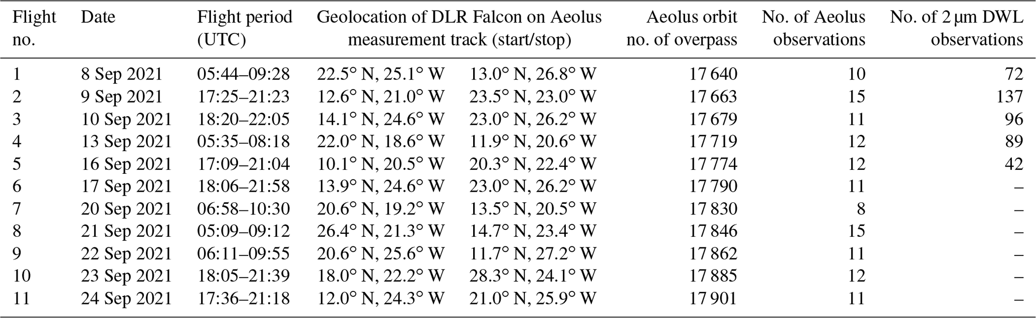
An overview of the 11 underpasses is provided in Table 1, including the geolocations of the start and end points of the respective sampled segment of the Aeolus path and the number of Aeolus and 2 µm DWL observations. While the number of 2 µm DWL observations corresponds to the number of wind profiles with a horizontal averaging length of about 8.8 km (one scanner revolution), one Aeolus observation is spread over a nominal horizontal averaging length of about 87 km. The latter is also referred to as basic repeat cycle (BRC) and can, in principle, contain multiple wind profiles, especially for the Mie channel, where the signals are typically averaged over 10 to 15 km, as a consequence of the grouping algorithm in the L2B processor (Rennie et al., 2020). Over the course of the campaign, the optical alignment of the 2 µm DWL was progressively degraded by the large temperature and humidity fluctuations in the aircraft during and between the flights, resulting in a significant reduction in the data coverage and, ultimately, operational failure toward the end of the campaign. Nevertheless, high-quality wind measurements were obtained from the first five underflights.
The colocated wind data served to assess the quality of the Aeolus wind product under the tropical atmospheric conditions in autumn 2021 with the goal to optimize the operational settings and to refine the retrieval algorithms for the operational phase of Aeolus and beyond. At that stage of the mission, the atmospheric path signal level, as measured with the Rayleigh channel, had decreased by around 50 % with respect to the signal levels detected during the AVATAR-I campaign in September 2019. The degradation in SNR was, however, partly mitigated by lower solar background levels in the tropics compared to the North Atlantic region, which also markedly influences the Rayleigh wind error (Rennie et al., 2021). The same is true for the Rayleigh-clear EE, as will be discussed in the following section.
2.2 The L2B EE and its temporal evolution
The horizontal line-of-sight (HLOS) wind error estimate is included in the Aeolus L2B product and calculated differently for the Rayleigh and Mie channels given the different measurement techniques for deriving the wind from the Doppler frequency shift. The Rayleigh channel relies on the double-edge technique (Chanin et al., 1989; Garnier and Chanin, 1992; Flesia and Korb, 1999; Gentry et al., 2000), where the shift in the broadband Rayleigh backscatter spectrum relative to the emitted spectrum is determined from the signal intensities that are transmitted through two bandpass filters (A and B). The filters are realized by sequential Fabry–Pérot interferometers (FPIs), with adequate spectral width and spacing with respect to each other, for obtaining high spectral sensitivity to small frequency shifts of a few megahertz. The temporal evolution of the filter parameters over the mission also allows insights into the instrument's alignment (Witschas et al., 2022b).
According to the L2B Algorithm Theoretical Basis Document (ATBD; Rennie et al., 2020), the EE for the Rayleigh HLOS wind speed is computed from the uncertainty in the Rayleigh spectrometer response R, which is defined as the contrast between the transmitted signals A and B, as follows:
The total signal that is incident on the Rayleigh detector (A+B), after being corrected for the solar background and the detector noise, is also referred to as the useful signal. The error in the Rayleigh response σR is related to the respective SNR values of filters A and B, which are provided in the L1B product and account for the Poisson noise of both the signal and the solar background. The latter is subtracted to obtain the atmospheric signal levels only. The response error is then given as follows (Rennie et al., 2020):
with
being the noise terms for the two FPI filters. The response error is converted to the Rayleigh HLOS wind speed EE σHLOS, R by considering the sensitivity of the Rayleigh spectrometer and the projection angle with the horizontal axis θ, i.e. the off-nadir angle of the instrument (θ≈37∘), as follows:
Assuming, without the loss of generality, that A=B, it can be followed from Eqs. (2) and (3) that
Hence, the Rayleigh EE scales with the reciprocal square root of the useful signal on the detector. Before launch, it was intended to include additional parameters in the HLOS wind EE computation for the Rayleigh channel to account for the (local) sensitivities of the derived LOS wind speed to atmospheric temperature and pressure, which influence the Rayleigh response (Dabas et al., 2008), and to the scattering ratio. However, these additional terms, which are formulated in the ATBD, are not considered in the current algorithm (up to baseline 14) due to the lack of dynamic values as an input for the respective error contributions. Furthermore, the noise that is introduced by the detector and read-out electronics is not accounted for in the EE calculation, although its contribution is not negligible in the case of low atmospheric signal levels, i.e. later in the mission. Consequently, the Rayleigh-clear EE is governed by the Poisson noise of the measured signal and the solar background. Note that it is foreseen that additional noise terms for the EE calculation will be included in future processor versions and, hence, reprocessed datasets.
The wind speed determination in the Mie channel is based on the fringe-imaging technique (McKay, 2002), where a linear interference pattern (fringe) is produced by a Fizeau interferometer and vertically imaged onto a detector. The Doppler frequency shift then manifests as a spatial displacement of the fringe peak position which changes approximately linearly with the frequency of the incident light. The peak position, which is referred to as the Mie response, is currently calculated by a Nelder–Mead downhill simplex algorithm (Nelder and Mead, 1965) to optimize a Lorentzian line shape fit of the signal distribution across the Mie channel detector (Mie Core algorithm; Reitebuch et al., 2018). The Mie channel EE is then related to the precision of the Mie response and is approximated from the solution error covariance of the fit algorithm, as described in the ATBD (Rennie et al., 2020). The covariance matrix is calculated from the partial derivatives of the Lorentzian line shape function with respect to four different fit parameters (peak position, peak height, peak width, and peak offset). An additional correction factor for each detector pixel accounts for the obscuration of the telescope primary mirror by the tripod that bears the secondary mirror (Tan et al., 2008). The error in the Mie response σM, i.e. the peak position error, is one element of the covariance matrix and can be converted to the Mie HLOS wind speed EE σHLOS, M as follows:
where λ is the laser wavelength, and m describes the Mie response slope, which is determined from a dedicated instrument calibration mode. Thus, the Mie EE is not directly linked to the atmospheric signal levels but rather depends on the signal distribution across the Mie detector and how well the peak from the imaged fringe resembles a Lorentzian line shape. The Mie signal distribution is, however, influenced by the broadband Rayleigh signal that is incident on the Fizeau interferometer and modifies the signal distribution, depending on its strength relative to the Mie peak and the illumination conditions. Moreover, since the fringe is coarsely resolved by only 16 pixels on the Mie detector (European Space Agency, 2008), the fit precision for the determination of its centroid position varies slightly, depending on how the fringe intensity is distributed among adjacent pixels (pixelation effect). The definitions of the L2B EE for the Rayleigh-clear and Mie-cloudy winds suggest that the values in the L2B product do not fully account for all error sources that affect the wind measurement in the two channels. It is also implied that the EE has been varying over the mission lifetime, as the atmospheric signal levels have been declining.
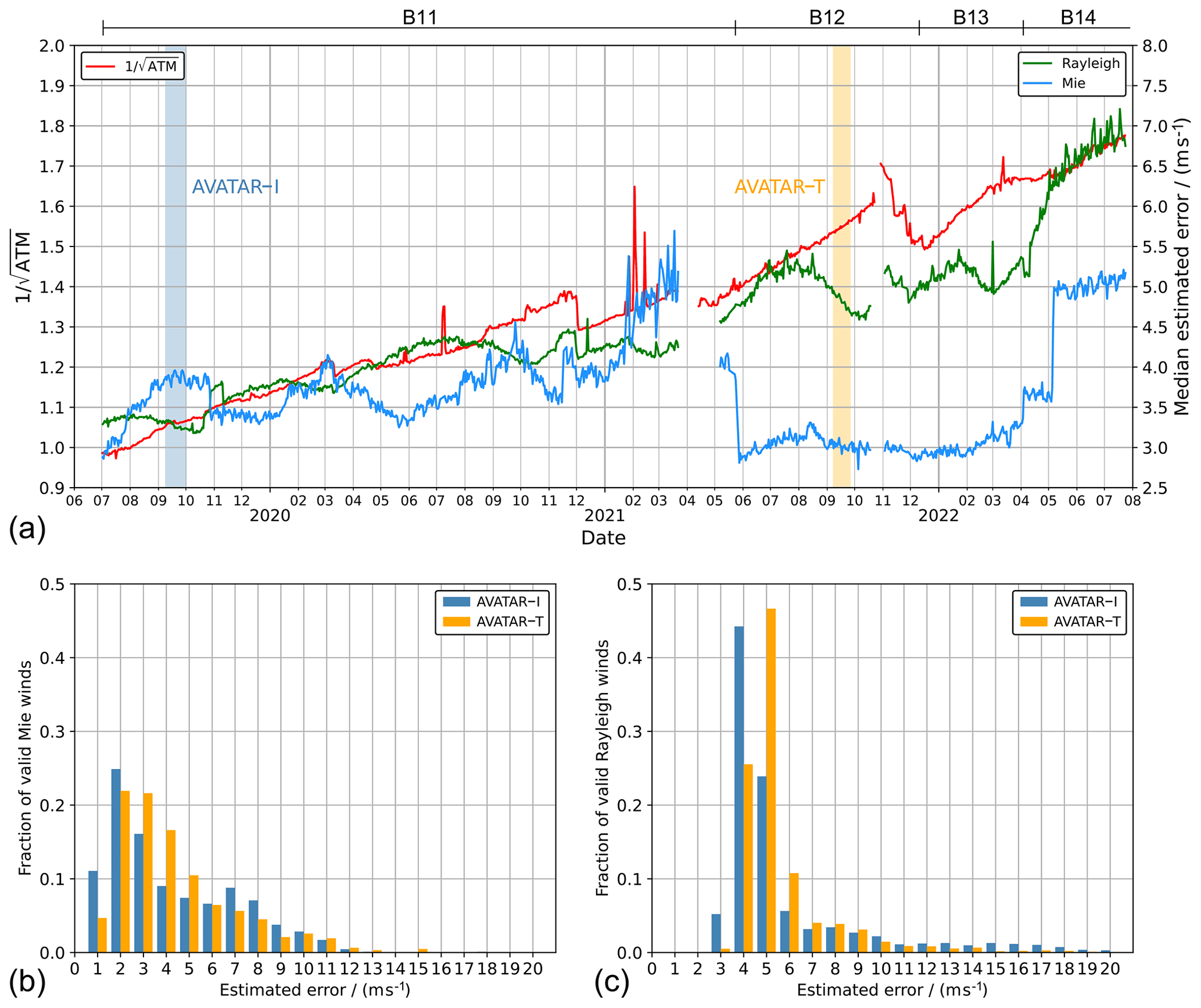
Figure 1Temporal evolution of the reciprocal square root of the of the atmospheric signal level () (red), normalized to the value from 26 July 2019, and the L2B Rayleigh-clear (green) and Mie-cloudy EE (blue) during the FM-B period (median per day). The baselines of the L2B product from which the data were extracted are indicated by the horizontal bars on the top of the plot. The lower panels depict the distribution of the Mie (b) and Rayleigh EE (c) for the periods and locations of the two DLR validation campaigns AVATAR-I (blue) and AVATAR-T (orange). The campaign periods are indicated by blue- and orange-shaded stripes in panel (a).
The temporal evolutions of the Rayleigh and Mie EE over the FM-B period are depicted in Fig. 1a. The green and blue curves represent the daily median of the global wind data extracted from the L2B product (baselines 11 to 14). The instrument was switched off for several weeks in March/April 2021 and October 2021, following two so-called Failure Detection Isolation And Recovery (FDIR) events, resulting in data gaps. The red line describes the long-term trend of the reciprocal square root of the atmospheric useful signal (), as measured with the Rayleigh channel under clear-sky conditions at about 10 km altitude, and normalized to the beginning of the FM-B period. The signal levels dropped by about 70 % between July 2019 and July 2022 ( increased from 1.0 to ), while intermittent signal increases can be attributed to instances in which the laser energy was boosted by special operations, e.g. in December 2020 and November 2021. The Rayleigh EE evolution roughly follows the trend of in accordance with Eq. (4), which assumes Poisson noise to be the dominant noise source (Reitebuch et al., 2018). The seasonal modulation of the Rayleigh EE is caused by the change in solar background noise, which adds to the shot noise of the signal and which is largest in the Northern Hemisphere summer, with secondary maxima in the Southern Hemisphere summer. The evolution of the Mie-cloudy EE is less affected by the signal trend and rather driven by the data processing algorithms and related settings which were modified several times over the FM-B period. Most notably, it was drastically reduced from around 4 to 3 m s−1 with the release of processor baseline 12 in May 2021. The latter involved a change in the L1B processor to ensure the correct summation of the raw Mie signals after dark current subtraction, without setting negative values to zero, leading to an improved fringe centroid computation and, in turn, a smaller random error and EE of the Mie winds. In early May 2022, the threshold settings of the Mie Core algorithm were relaxed to obtain more valid Mie winds of reasonable quality at the expense of more outliers with high EE, hence increasing the median to around 5 m s−1.
The variability in the EE also becomes obvious when comparing its distribution for two datasets from different periods and geographical locations. Figure 1b shows the histograms of the Mie EE that was extracted from the L2B product for the 10 Aeolus underflights of the AVATAR-I campaign in the North Atlantic in September 2019 (blue bars) and for the 11 underflights of the AVATAR-T campaign in the tropics in September 2021 (orange bars). For the latter dataset, the portion of Mie winds with EE ranging from 3 to 6 m s−1 is significantly larger than for the AVATAR-I dataset, which, however, contains more Mie winds with EE smaller than 3 m s−1 and larger than 6 m s−1. Regarding the Rayleigh channel (Fig. 1c), the EE distribution has shifted towards higher values in accordance with the overall trend shown in Fig. 1a, although the impact of the atmospheric signal decrease between the two campaigns on the EE was partially compensated by the smaller detrimental influence of the solar background in the tropics compared to the higher latitudes and the fact that the range bin thickness was set to be larger (750 compared to 500 m during AVATAR-I).
Given the change in the EE distributions over the FM-B period, the rejection of wind results by using a (fixed) EE threshold as QC would lead to different portions of winds from the respective dataset to be validated and, hence, misleading results when comparing and interpreting the statistics of error distributions for the two campaigns. Therefore, it is crucial to consider the influence of different EE thresholds on the validation results and to find alternative schemes for the QC of the Aeolus data.
The investigation of different QC schemes will be presented based on the statistical comparison of L2B wind results against model background winds from the 11 underflight legs of the AVATAR-T campaign, as summarized in Table 1. The model background wind data, which serve as the reference, are contained in the Aeolus auxiliary meteorological file (AUX_MET). It includes vertical profiles (137 pressure levels) of ECMWF operational model fields from a short-range forecast run of up to 12 h at TCo 1279 (for triangular–cubic-octahedral) resolution (∼9 km grid) along the predicted ground track of Aeolus for both nadir and off-nadir pointing (Rennie et al., 2020). Note that the model wind data are independent of the Aeolus winds, as they are produced before assimilation of the latter (Aeolus winds were assimilated in the previous model runs, though). The AUX_MET data (zonal and meridional wind components) were averaged onto the L2B grid by means of a weighted aerial interpolation algorithm (Marksteiner, 2013), which was also applied for the harmonization of the L2B and A2D datasets in previous airborne campaigns (Lux et al., 2018, 2020a, 2022). This procedure allows for a direct comparison of each L2B wind observation (O) against the averaged model background (B), resulting in so-called “observation minus background” (O-B) statistics (Rennie et al., 2021; Marseille et al., 2022).
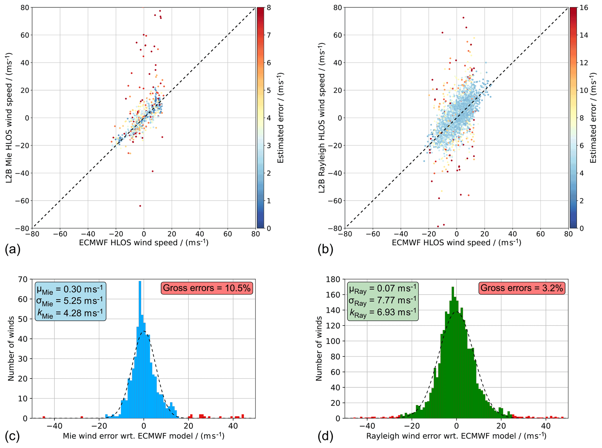
Figure 2Scatterplots comparing the L2B Mie-cloudy (a) and Rayleigh-clear (b) wind results against ECMWF model winds from the 11 underflights of the AVATAR-T campaign. The colour-coding describes the L2B EE of the wind results. The statistical parameters without and with outlier removal, using the modified Z score, are given in Table 2. (c, d) Histograms of the respective wind errors (L2B minus ECMWF model) in bins of 1 m s−1. The red bars indicate gross errors, as identified by the modified Z score. The dashed lines represent Gaussian fits of the error distributions after outlier removal. The statistical parameters after outlier removal are given in the insets.
3.1 Systematic and random wind error
The statistical results from the model comparison without applying any QC are depicted in Fig. 2 for the Mie-cloudy (Fig. 2a, c) and the Rayleigh-clear wind results (Fig. 2b, d). The scatters in the top plots are colour-coded according to the respective EE value that is assigned to each wind result. Overall, the L2B wind results show good agreement with the model background winds from the ECMWF; however, there are quite a few wind results with large departures from the model, particularly for the Mie channel. Those winds are very often, but not always, associated with a large EE. The bottom plots represent the histograms, or probability density functions (PDFs), of the respective (O-B) wind errors, i.e. L2B minus ECMWF model. The histograms are nearly Gaussian distributed, when excluding the large outliers that are indicated by the red bars and whose identification will be discussed below. The main output of the analysis is the three statistical parameters that are listed in the inset boxes. The systematic wind error, or mean bias, with respect to the ECMWF model background is calculated as follows:
It represents the mean of the wind speed differences between Aeolus and the model, with n being the number of comparable winds after the exclusion of outliers.
The random error is given in terms of the standard deviation, as follows:
Additionally, the scaled median absolute deviation (scaled MAD) is derived as follows:
The scaled MAD is more resilient to outliers in the dataset and thus a more robust measure of the wind error variability than the standard deviation. In case the analysed data are normally distributed, the standard deviation and scaled MAD are identical.
The definitions given here are in line with the those stated in the Aeolus MRD, which assumes that the wind error with respect to other wind observations or the model background can be described by a Gaussian distribution, whose centre and width represent the accuracy and precision of the Aeolus winds. This is justified by the fact that the wind error is dominated by Poisson-distributed photon noise on the detectors, particularly for the Rayleigh channel. For the Mie channel, deficiencies in the signal analysis (Mie Core algorithm) give rise to gross errors which additionally contribute to the error distribution, as will be pointed out in Sect. 3.3. Nevertheless, after sorting out the gross errors, the assumption of a Gaussian distribution is also valid for the Mie channel.
3.2 Modified Z score for outlier detection
Data can be screened for outliers by calculating the modified Z score1 for each wind observation. It describes its distance from the median, measured in units of the scaled MAD, as follows (Iglewicz and Hoaglin, 1993):
with k denoting the scaled MAD, as introduced in Eq. (7). Since the median and the scaled MAD are more robust to outliers compared to the mean and standard deviation, the modified Z score is a valuable tool for data screening, even if the distribution is far from Gaussian and/or the dataset is small. Iglewicz and Hoaglin (1993) recommended that modified Z scores with an absolute value greater than 3.5 are to be labelled as outliers. However, thresholds of 3 or even smaller are also used in literature, depending on the convention for defining outliers (Tripathy, 2013; Sandbhor and Chaphalkar, 2019).
Table 2Statistical comparison of the Aeolus L2B Mie-cloudy and Aeolus L2B Rayleigh-clear winds against the ECMWF model background winds for all underflights performed during the AVATAR-T campaign. The corresponding scatterplots and histograms are shown in Figs. 2 and 3, respectively. The statistics are derived after the adaptation of the ECMWF model data to the respective L2B measurement grids. The statistical parameters are given without and with the removal of outliers according to the modified Z score (|Zm|>3.5).
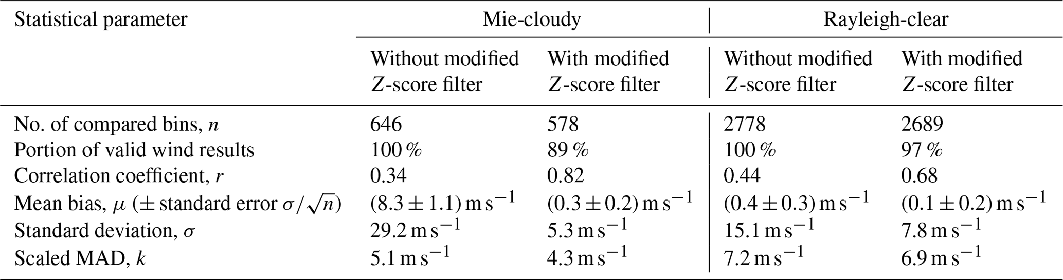
Following the recommendation from Iglewicz and Hoaglin (1993), the (O-B) wind errors with respect to the ECMWF model background were filtered based on the modified Z score, i.e. wind results for which |Zm| is greater than 3.5 were removed from the dataset. For the Mie-cloudy winds, 10.5 % outliers (68 out of 646 wind results) were identified in this manner, while the portion is much smaller for the Rayleigh-clear winds (89 outliers out of 2778 wind results; ≈3.2 %). The outlier removal has a significant impact on the derived statistical parameters (see Table 2), especially for the Mie channel. Since most of the Mie wind outliers are positively biased, the systematic error is as high as 8.3 m s−1 if no QC is applied, but it is reduced to 0.3 m s−1 by the outlier rejection based on the modified Z score. At the same time, the standard deviation is drastically decreased from 29.2 to 5.3 m s−1. The impact on the scaled MAD is much smaller (5.1 to 4.3 m s−1) because it is less prone to outliers, as described above. Regarding the Rayleigh statistics, the biggest effect of the outlier removal is observed for the standard deviation, which is reduced from 15.1 to 7.8 m s−1, while the mean bias (0.4 to 0.1 m s−1) and the scaled MAD (7.2 to 6.9 m s−1) are only slightly affected. The reason is the much more homogeneous distribution of outliers outside of the nearly Gaussian distribution as opposed to the Mie winds (see Fig. 2c and d), so that the rejection of winds with |Zm|>3.5 mainly leads to a narrowing of the error distribution without changing its centre of mass.
Note that the Z-score filter is sufficiently relaxed to avoid the rejection of wind observations that might be due to extreme wind occurrences. Taking the scaled MAD values for the Mie and Rayleigh winds before applying the filter (5.1 and 7.2 m s−1, respectively) and considering that the median of the wind speed differences is close to zero, only wind results that deviate by more than ≈18 m s−1 (Mie) or ≈25 m s−1 (Rayleigh) from the model are considered to be outliers. This is well above typical model errors that are caused by deficiencies in terms of parametrization and resolution and can, in extreme cases, like in highly convective regions, exceed 10 m s−1 (Rennie et al., 2021).
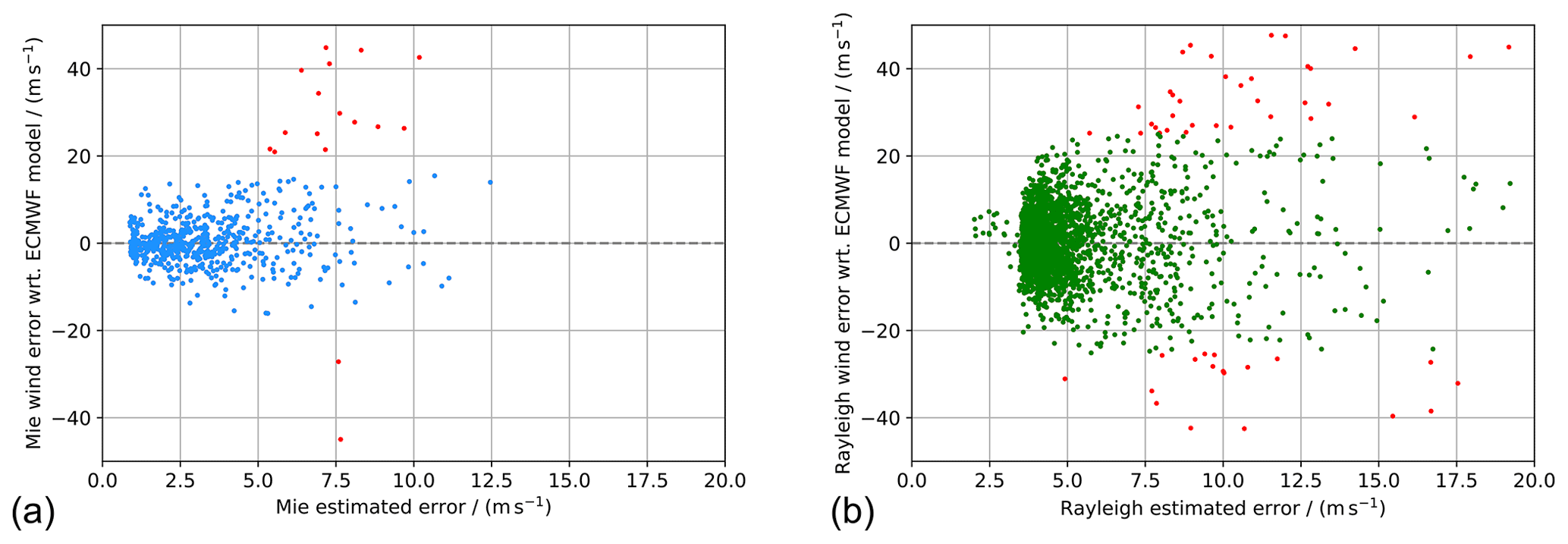
Figure 3L2B Mie-cloudy (a) and Rayleigh-clear (b) wind error with respect to the ECMWF model background winds vs. the L2B EE for the 11 underflights of the AVATAR-T campaign. The red data points represent outliers, as identified by the modified Z score (|Zm|>3.5). Note that there are many more Mie outliers with errors greater than ±50 m s−1.
The differences in the outlier distributions also become obvious when plotting the (O-B) wind error against the EE of the respective wind product (Fig. 3). At higher EE, the number of winds with larger error with respect to the model increases, as expected. However, while the larger Rayleigh wind errors are almost evenly distributed, there is a preponderance of Mie outliers with a positive bias relative to the model background. Note that the Mie data include many more outliers with errors greater than ±50 m s−1, which are not displayed in Fig. 3a for the sake of readability. One of these extreme outliers, with a wind error of 146 m s−1, has an EE of only 5.6 m s−1. This outlier would spoil the Mie statistics at a moderate EE threshold of 5.6 m s−1, unless an additional QC scheme, such as the modified Z score, is applied to the dataset. Conversely, there are several winds with a small error, with respect to the model, but high EE. Some of these low-error winds are, however, non-physical results and merely part of the random wind distribution around the reference model wind, especially for the Rayleigh channel (see also Fig. 2a and b).
3.3 Mie gross errors
Outliers that are not represented by a Gaussian distribution can be referred to as gross errors and are usually caused by data transmission or instrument failure. In the case of the Aeolus Mie-cloudy winds, gross errors generally originate from the false detection of a Mie fringe by the Mie Core algorithm, especially at weak particulate backscatter signals when the Rayleigh background or other noise sources may produce a small peak on the Mie detector, which is then erroneously registered as a fringe. This results in non-physical wind speeds with large departures from the actual wind, depending on the position of the peak, which is also determined by the illumination conditions of the Fizeau interferometer and thus by the telescope obscuration along the orbit. As shown in Fig. 3a, such gross errors are not reliably assigned an adequately large EE to be filtered out accordingly by common QC methods.
Experience with conventional observation systems and associated instrument and retrieval QC settings in operational meteorological analysis suggest that the rate, or probability, of gross errors present in the analysis (after QC) should not exceed a few percent to avoid deterioration of the NWP skill (Lorenc and Hammon, 1988). This is also important to prevent random wind estimates that are, by coincidence, close to the true wind from influencing the analysis. Consequently, in addition to specifying the required wind random error for the Mie and Rayleigh winds in different altitude ranges, the Aeolus MRD contains a gross error requirement, which states that the probability of gross errors shall be less than 5 % within a wind speed range of 6 times the random error requirement (6σ), while no gross errors shall be present outside of this wind speed range (European Space Agency, 2016). The gross error requirement is only applicable to the Mie channel, whereas it is already covered by the random error requirement for the Rayleigh channel, where the noise sources are assumed to be purely Gaussian.
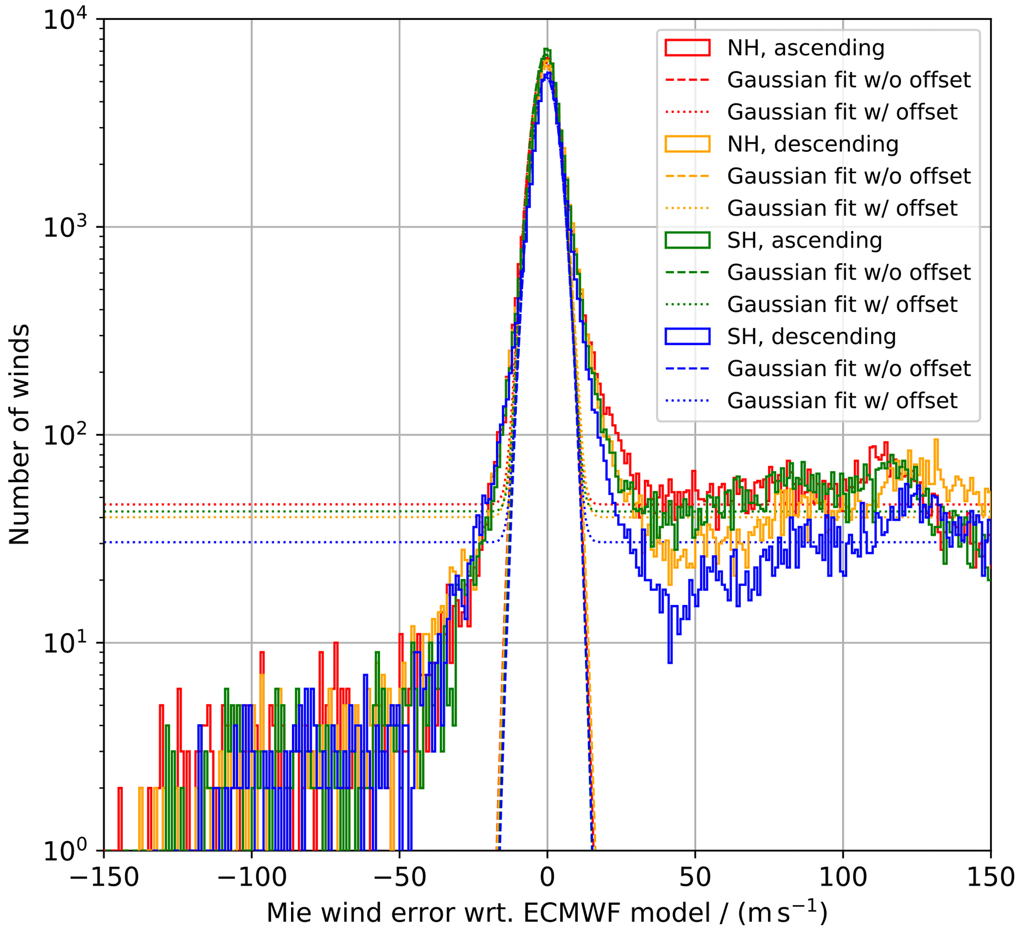
Figure 4Histograms of the L2B Mie-cloudy wind error against ECMWF model background data from the period between 20 and 25 March 2022 for the Northern/Southern hemispheres and ascending/descending orbits. The dashed and dotted lines represent Gaussian fits without and with offset, respectively.
Before launch, it was assumed that the Mie gross errors are uniformly distributed so that, in principle, the increase in random error caused by the gross errors within the 6σ range is less than 5 % (European Space Agency, 2016). However, analysis of the Mie-cloudy wind data after launch revealed a strongly asymmetric distribution of gross errors, with a predominance of positively biased winds, as shown in the previous section. This fact becomes even more obvious when regarding larger datasets. Figure 4 depicts histograms of the (O-B) Mie wind error (in logarithmic scale) from 5 d of data (from 20 through 25 March 2022), subdivided into four groups depending on the geographical location (Northern and Southern hemispheres, NH/SH) and the orbital node of the satellite (ascending and descending). Gaussian fits without and with an offset term are represented as dashed and dotted lines for each data subset, respectively. Due to the complex gross error distribution, which differs among the subsets and features multiple local maxima along the wind error range, the contribution of non-Gaussian errors cannot be approximated by a simple analytic function, e.g. by a constant offset, as assumed before launch, or by a linear relationship. Therefore, the use of a Gaussian fit with offset is not considered useful to describe the Mie wind error distribution including gross errors, as opposed to the pre-launch assumptions. Instead, QC should be performed such that the resulting wind error distribution is as close to a Gaussian distribution (without offset) as possible. However, when using this approach, one accepts the inclusion of non-physical wind observations that, by chance, fall within the Gaussian distribution. A convenient method to assess to what extent a given dataset follows a Gaussian distribution is provided by normal quantile plots which are introduced in the next section.
3.4 Normal quantile plots
Normal quantile plots are a graphical tool for evaluating whether or not a dataset is approximately normally distributed (Chambers et al., 1983). They represent a special case of quantile–quantile plots (QQ plots), where the probability distribution of observed (empirical) data are compared to a specified theoretical distribution by plotting their quantiles against each other. A linear pattern of the scattered points suggests that the measured distribution is reasonably described by the theoretical, e.g. Gaussian, distribution, while departures from a straight line indicate deviations from normality. Usually, a reference line is added to the plot which passes through the first (Q25) and third quartiles (Q75) of the distributions, denoting the values that cut off the first and last quarter of the data when it is sorted in ascending order. The residuals from this reference line are then a measure of the non-normality. The residuals can be measured either in quantiles or in units of the quantity plotted by considering the mean and standard deviation of the sample distribution. A normal quantile plot can be interpreted less ambiguously than a histogram, and the shape of the curve allows conclusions to be drawn about the skewness and kurtosis of the distribution.

Figure 5Normality check of the Rayleigh-clear wind error distribution from the ECMWF model comparison based on the AVATAR-T dataset for two different QC approaches. (a, b) Histograms of the Rayleigh wind error with respect to the ECMWF model background (a) after QC based on an EE threshold of 10 m s−1 and after QC based on the modified Z score (|Zm|>3.5). The vertical dashed lines indicate the first and third quartiles of the given (sample) distribution (Q25s; Q75s) and the theoretical normal distribution used for comparison (Q25n; Q75n). The corresponding parameters are also visualized as horizontal and vertical dashed lines (quartile lines) in the normal quantile plots for the two QC approaches plotted in panels (c) and (d), respectively. The quartile reference line (red), which is defined by the intersection points of the quartile lines, is used to calculate the residual quantiles which are depicted in panels (e) and (f).
The use of a normal quantile plot is demonstrated using the example from Sect. 3.1, i.e. the validation of L2B Rayleigh-clear winds against ECMWF model background data from the AVATAR-T campaign (see Fig. 2b and d). Two different QC schemes were applied to study their influence on the normality of the resulting wind error distribution. The first QC corresponds to the widely used approach where L2B winds for which the EE exceeds a certain value are filtered out. Here, a threshold of 10 m s−1 was chosen, which is slightly larger than the most commonly used value of 8 m s−1, but is regarded as an appropriate threshold given the increased noise levels during the campaign compared to the start of the FM-B and elevated EE of the Rayleigh winds accordingly (see Fig. 1). The second QC is based on the modified Z score, discarding those winds for which |Zm|>3.5. The corresponding histograms are displayed in Fig. 5a and b, with the red bars indicating the data that are removed by the respective QC scheme. While the EE approach rejects 5.5 % of the wind results across the entire wind error range, the QC that relies on the modified Z score (by design) only removes data from the far edges of the distribution. As a consequence, the normal quantile plot for the second approach, which is depicted in Fig. 5d, shows smaller departures from the reference line compared to the EE approach (Fig. 5c). The residuals from the reference line are plotted in the bottom row of Fig. 5, revealing large deviations from normality for the first QC scheme, particularly on the edges. The flipped S-shape of the curve suggests a so-called heavy-tailed distribution of the wind errors, i.e. the existence of large outliers. In other words, the QC scheme based on the EE threshold does not completely remove all the Rayleigh gross errors, so that the resulting (O-B) wind error distribution is not Gaussian, as it is required for a proper assessment of the L2B wind error according to the MRD. In contrast, when using the modified Z score for QC, the wind error distribution (O-B) shows much higher normality with residuals smaller than 1σ (see the grey-shaded area in Fig. 5f), while retaining a higher fraction of valid winds (close to the median) in the dataset.
Although the modified Z score is a useful technique for increasing the normality of a given dataset, it should be noted that the choice of the Z score threshold is crucial. If the chosen limit is too small, e.g. |Zm|>2, then a significant portion of the wings of the error distribution is cut off, resulting in a light-tailed distribution which manifests as an S-shaped curve in the normal quantile plot and, hence, decreased normality. For the model comparison of Rayleigh-clear winds, a Z score limit ranging from 3.0 to 3.5 was found to yield a high degree of normality, which is in accordance with the recommendation by Iglewicz and Hoaglin (1993). Concerning the Mie-cloudy winds, the situation is more complicated due to the pronounced asymmetry in the gross error distribution which even affects the outlier-robust median and scaled MAD and, hence, the modified Z score. Therefore, the combination of an EE threshold and a modified Z-score filter is suggested as a reasonable QC approach, as will be elaborated on in Sect. 4. Prior to that, the influence of various QC settings on the statistical results of the model comparison is presented in the following section.
3.5 Influence of the QC on the validation results
The evaluation of the Aeolus wind data quality is predicated on the determination of the systematic (accuracy) and random error (precision) of the wind results in the L2B data product. These key parameters are described by the mean bias μ (Eq. 6) and standard deviation σ (Eq. 7) with respect to the reference instrument or model data. The scaled MAD k (Eq. 8) is sometimes calculated as an additional measure of the wind precision, although it is not compliant with the random error definition that is formulated in the MRD. Note that, in case of a normally distributed (O-B) wind error, the scaled MAD is identical to the standard deviation, and a distinction between the two parameters is obsolete. In this sense, the degree of deviation between k and σ is another measure of non-normality.
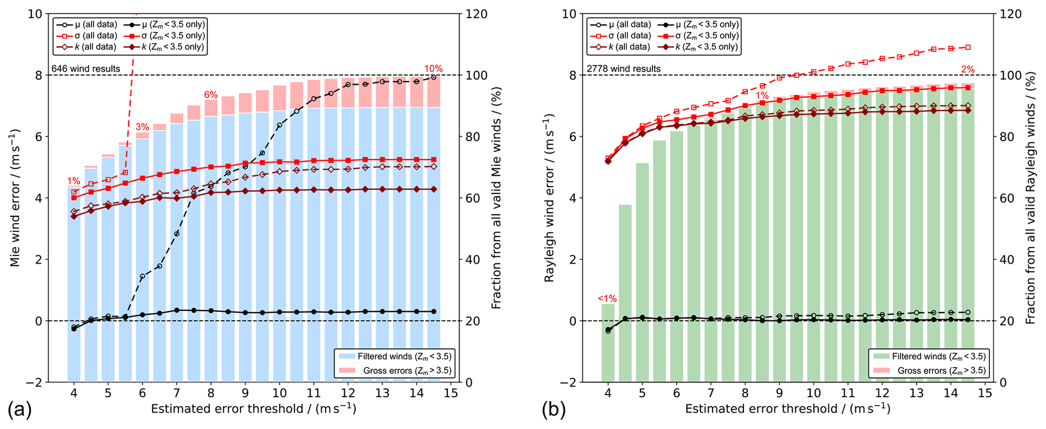
Figure 6Results from the statistical comparison of L2B Mie-cloudy (a) and Rayleigh-clear winds (b) against ECMWF model background wind data from the AVATAR-T campaign, depending on the EE threshold without and with outlier removal based on the modified Z score. The bar plots depict the portion of filtered winds after QC (|Zm|<3.5; blue and green bars) and gross errors (|Zm|>3.5; red bars) from all wind results that are flagged valid in the L2B product and pass the specified EE threshold. The portion of gross errors is indicated above the bars. The dashed lines and open symbols refer to the statistical results (mean bias μ, standard deviation σ, and scaled MAD k) without removing the gross errors from the datasets, while the solid lines represent the statistical parameters after QC based on the modified Z score.
The statistical parameters are strongly influenced by the applied QC approach and related threshold settings, which also determine the fraction of wind results (with validity flag = 1) that are discarded from the original dataset. For the purpose of summarizing the impact of the chosen QC settings on the validation results, a combined bar and line graph was developed, as depicted in Fig. 6, for the error assessment of the Mie-cloudy and Rayleigh-clear winds against the ECMWF model background data from the AVATAR-T campaign. The diagram intends to give an overview of the most relevant statistical parameters (μ, σ, k, and fraction of valid winds that is considered in the statistics) dependent on the chosen EE threshold. The x axis denotes the EE threshold up to which winds results are retained in the dataset. The left y axis refers to the plotted lines which describe the mean bias (circles), standard deviation (squares), and scaled MAD (diamonds). The statistical parameters are calculated for two cases, i.e. without and with the additional application of a modified Z-score filter (|Zm|<3.5), represented by the dashed and solid lines, respectively. The bar chart, referring to the right y axis, indicates the percentage of valid data that are included in the statistical analysis, whereby the red columns specify the portion of wind results that are rejected by the modified Z-score filter. Note that the L2B product also contains Rayleigh-clear winds with EE >15 m s−1 (≈3 %), reaching even EE values beyond 100 m s−1, so that the columns in Fig. 6b do not reach 100 %, as opposed to the Mie-cloudy winds depicted in Fig. 6a, where the maximum EE is 14.7 m s−1.
The plot in Fig. 6a demonstrates that the QC based on the EE threshold rejects almost 40 % of the valid Mie winds at a threshold of 4 m s−1 (which is often used in validation studies), while this portion is reduced to less than 20 % when the threshold is relaxed to 6 m s−1. At the same time, multiple large outliers are added to the analysed dataset, including the one with 146 m s−1 mentioned before, and strongly affect the mean bias (from 0.1 to 1.4 m s−1) and standard deviation (from 4.5 to 12.9 m s−1), while the scaled MAD is only slightly increased from 3.7 to 4.0 m s−1. Consequently, solely using the EE as a QC parameter implies that either a large portion of data is discarded or several Mie gross errors are included in the dataset that distort the statistics. In both cases, the validation results become less significant, especially if the original dataset is already small, e.g. in ground-based campaigns with only a few Aeolus overpasses to be analysed.
A solution to this problem is offered by the modified Z-score filter, which sorts out the gross errors and hence permits higher EE thresholds. Using a threshold of 6 m s−1 and removing the aforementioned outliers by a subsequent QC step based on the modified Z score (|Zm|<3.5) retains 80 % of all valid winds in the dataset, while ensuring robust statistical parameters (μ=0.2 m s−1, σ=4.6 m s−1, and k=3.9 m s−1). The latter are changed to some extent when the EE threshold is further increased up to a point where all valid Mie winds pass the first QC step and only the modified Z-score filter takes effect, rejecting ≈10 % of the data which are identified as gross errors. The resulting values (μ=0.3 m s−1, σ=5.3 m s−1, and k=4.3 m s−1) represent the statistics shown in Fig. 2c and Table 2.
Regarding the Rayleigh-clear wind results, the impact of an additional Z-score filter is less striking, owing to the much more homogeneous distribution of the outliers, as explained in the previous sections. At a typical EE threshold of 8 m s−1 (Witschas et al., 2020), about 90 % of all valid winds pass the first QC step, including less than 1 % of outliers. The latter hardly affect the statistical parameters. The systematic error changes from 0.10 to 0.03 m s−1, while the standard deviation and the scaled MAD decrease from 7.5 to 7.0 m s−1 and from 6.7 to 6.6 m s−1 upon the application of the modified Z-score filter, respectively. When the EE threshold is more and more relaxed, eventually switching off the EE-based QC, the influence of 3 % of outliers in the dataset becomes more pronounced, so that the modified Z-score filter is also useful for the Rayleigh winds, reducing the mean bias from 0.43 to 0.07 m s−1, the standard deviation from 15.1 to 7.8 m s−1, and the scaled MAD from 7.2 to 6.9 m s−1 (see also Table 2).
To conclude, the modified Z score is an effective method to discard gross errors from the L2B data that are detrimental to the validation results, thus enabling higher EE thresholds and, in turn, larger portions of valid winds to be included in the statistical analysis. This is particularly true for the Mie-cloudy winds, where extreme (mainly positively biased) outliers with small EE may occur in the dataset, which, if not properly rejected, lead to a strongly skewed wind error distribution. The choice of the Z score limit, however, remains arbitrary and may have a non-negligible influence on the statistical results, depending on the actual dataset that is used for the validation of the L2B winds. For the model comparison discussed above, the statistical parameters change by less than 7 % if the Z score limit is reduced from 3.5 to 3.0. The largest influence is found for the Rayleigh standard deviation, which decreases to 7.3 m s−1 (compared to 7.8 m s−1 for a Z score limit of 3.5), as the portion of outliers accounts for 4.5 % (compared to 3.2 %).
The statistical methods introduced in Sect. 3 will now be exemplarily applied in an Aeolus validation study based on the 2 µm DWL, which was deployed during the AVATAR-T campaign aboard the DLR Falcon aircraft. Thanks to a double-wedge scanner, the 2 µm DWL is capable of measuring the range-resolved three-dimensional wind vector with a mean accuracy of ≈0.1 m s−1 and a mean precision of better than 1 m s−1 (Weissmann et al., 2005; Witschas et al., 2017). For comparing the 2 µm DWL winds to the L2B wind data, the measured wind vector is projected onto the Aeolus HLOS axis, while averaging procedures are performed to account for the different horizontal and vertical resolutions of the 2 µm DWL (≈8.8 km; 100 m) and Aeolus (≈87 km for Rayleigh and 10 km for Mie; 0.25 to 2 km), as explained in Witschas et al. (2020). The 2 µm DWL delivered high-quality wind observations during the first five AVATAR-T underflights (see Sect. 2.1), enabling the validation of 563 Rayleigh-clear and 162 Mie-cloudy winds in case no further QC in addition to the validity flag is applied.
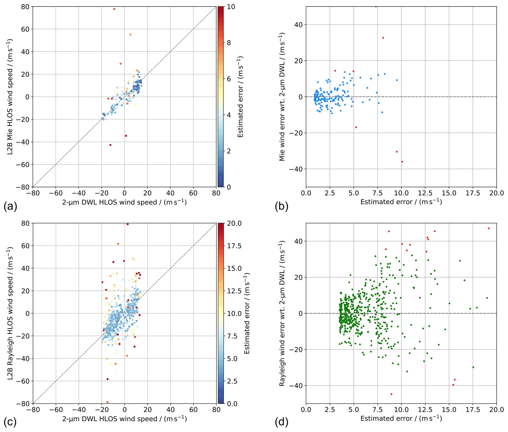
Figure 7(a) Scatterplots comparing the L2B Mie-cloudy wind results against 2 µm DWL winds (projected onto the horizontal viewing direction of Aeolus) from the 11 underflights of the AVATAR-T campaign. The colour-coding describes the L2B EE of the wind results. (b) Mie-cloudy wind error with respect to the 2 µm DWL winds vs. the L2B EE. The red data points represent outliers as identified by the modified Z score (|Zm|>3.5). The bottom panels (c) and (d) depict the corresponding plots for the L2B Rayleigh-clear wind results.
The results of the statistical comparison are shown in Fig. 7. In analogy to Fig. 2, the scatterplots in Fig. 2a and c depict the correlation of the Mie-cloudy and Rayleigh-clear winds against 2 µm DWL wind data, respectively, with the colour-coding describing the EE. Scatters with a larger departure from the 1:1 line in most cases exhibit a high EE, suggesting that the latter parameter is a decent proxy for the wind data quality. However, there are also several outliers with comparatively small EE and several Aeolus wind results with good agreement to the 2 µm DWL but large EE. The presence of outliers, as defined by a modified Z score exceeding 3.5, is visualized in Fig. 2b and d for the two receiver channels. Out of a total number of 11 Mie outliers, five are not displayed in the graph because the departures are greater than +50 m s−1, again demonstrating the strongly skewed wind error distribution for the Mie channel. The number of Rayleigh wind errors with |Zm|>3.5 (27) accounts for around 5 % of all valid wind results, with a small preponderance of positive deviations from the 2 µm wind speeds.

Figure 8Same as Fig. 6 but for the statistical comparison of L2B Mie-cloudy (a) and Rayleigh-clear winds (b) against 2 µm DWL wind data. The EE thresholds that are deemed reasonable for providing robust statistical results are highlighted by orange frames (see also Fig. 9).
The influence of the previously discussed QC schemes (EE threshold in combination with modified Z score) on the key statistical parameters is illustrated in Fig. 8. In accordance with the model comparison shown in Fig. 6, the systematic and random error in the Aeolus L2B wind results with respect to the 2 µm DWL wind data increase as the EE threshold is relaxed, whereby larger departures are evident without the application of an additional modified Z-score filter (dashed lines), as expected. The percentage of outliers that are identified by the modified Z score is comparable to the validation against the ECMWF model background (Mie is ≈7 %; Rayleigh is ≈3 %). This result confirms the fact that the Mie-cloudy winds do not fulfil the gross error requirement formulated in the MRD (Sect. 3.3), since the contribution of non-Gaussian error sources is larger than 5 %. Moreover, there exist multiple gross errors outside of the 6σ range ( m s−1), including wind results with departures from the 2 µm DWL winds of more than 50 m s−1, as mentioned above. Therefore, it is recommended to refine the Aeolus L1B and L2B processors, i.e. the Mie Core algorithm threshold settings, in order to eliminate all gross outliers outside of the 6σ range and, hence, to avoid an overestimation of the Mie random error.
Interestingly, the EE thresholds at which the portion of winds that are considered in the statistics (blue and green bars in Fig. 8) exceeds 80 % differ from the results of the model comparison for the Mie and the Rayleigh channel. In the latter case, EE thresholds of at least 6 m s−1 are necessary to reach the 80 % mark for both channels (Fig. 6). In contrast, it would, in principle, be sufficient to choose an EE threshold of 4.5 m s−1 for the Mie winds, whereas the EE threshold for the Rayleigh winds has to be as high as 8.5 m s−1 when comparing them against the 2 µm DWL data. This can presumably be explained with the spatial overlap of the 2 µm DWL wind with the data of the two channels. Since the heterodyne detection lidar primarily measures winds from particulate backscatter (aerosols and clouds), it mainly covers regions where high-quality Mie winds are expected. Thus, a large portion of valid Mie winds that overlap with the 2 µm DWL wind data show low EE. Nevertheless, thanks to its high sensitivity, the 2 µm DWL is also capable of measuring winds in regions with scattering ratios as low as 1.01, and hence, there is a high availability of Rayleigh-clear winds. Since areas with low cloud coverage are targeted for the Aeolus underflights for the purpose of high wind data coverage, there are more Rayleigh-clear than Mie-cloudy winds to be validated by the 2 µm DWL. Most of the Rayleigh winds overlapping with the 2 µm DWL data coverage, however, stem from extended aerosol layers in the lower troposphere, including the planetary boundary layer (PBL) in the lowermost 2 km with shorter-range bins (500 compared to 750 m). This region is characterized by increased EE values owing to the attenuated molecular backscatter and thus reduced SNR. Higher-quality Rayleigh winds with low EE, which are prevalent in the middle and upper troposphere in clear-sky conditions (scattering ratio of well below 1.01), are underrepresented in the validation dataset so that a higher EE threshold is necessary to obtain the same portion of valid Rayleigh winds as for the model comparison.
These considerations emphasize the importance of a comprehensive statistical analysis for assessing the Aeolus wind errors. Depending on the characteristics of the reference instrument (data coverage, resolution, etc.), the EE threshold has to be chosen such that a significant portion, e.g. 80 %, of the wind data is included in the statistics. This is particularly true if the wind data quality is evaluated over longer time periods, given the long-term variability in the EE (Fig. 1).
Following this criterion, the Rayleigh EE threshold was set to 8.5 m s−1 for the validation against the 2 µm DWL data, resulting in a mean bias of μ=0.2 m s−1, standard deviation of σ=8.8 m s−1, and scaled MAD of k=7.3 m s−1, if no further QC is applied. When removing outliers by means of the modified Z score, which account for 1.1 % of the data, the parameters are changed to m s−1, σ=8.2 m s−1, and k=7.2 m s−1, respectively. Note that, if the EE threshold was relaxed further, the random error would significantly increase to more than 10 m s−1, which is in contrast to the model comparison where it remains almost constant at around 8 m s−1. The reason is most likely the fact that the Rayleigh-clear wind results with higher EE that were validated by the 2 µm DWL are largely located in dust-laden areas, including the PBL, where the shorter-range bin thickness leads to lower SNR in addition to the attenuation by aerosols. This topic is discussed in more detail by Witschas et al. (2022a).
Apart from the portion of wind data that passes the QC, other criteria should be considered for selecting an appropriate EE threshold. For instance, as pointed out in Sect. 3.5, the difference between σ and k represents a good measure of the non-normality of the wind error distribution. Hence, the EE threshold could be chosen such that the deviation between the two parameters is, for instance, below 1 m s−1. This condition is fulfilled when applying the QC settings for the Rayleigh winds given above (EE threshold is 8.5 m s−1 and modified Z-score filter with a limit of 3.5).
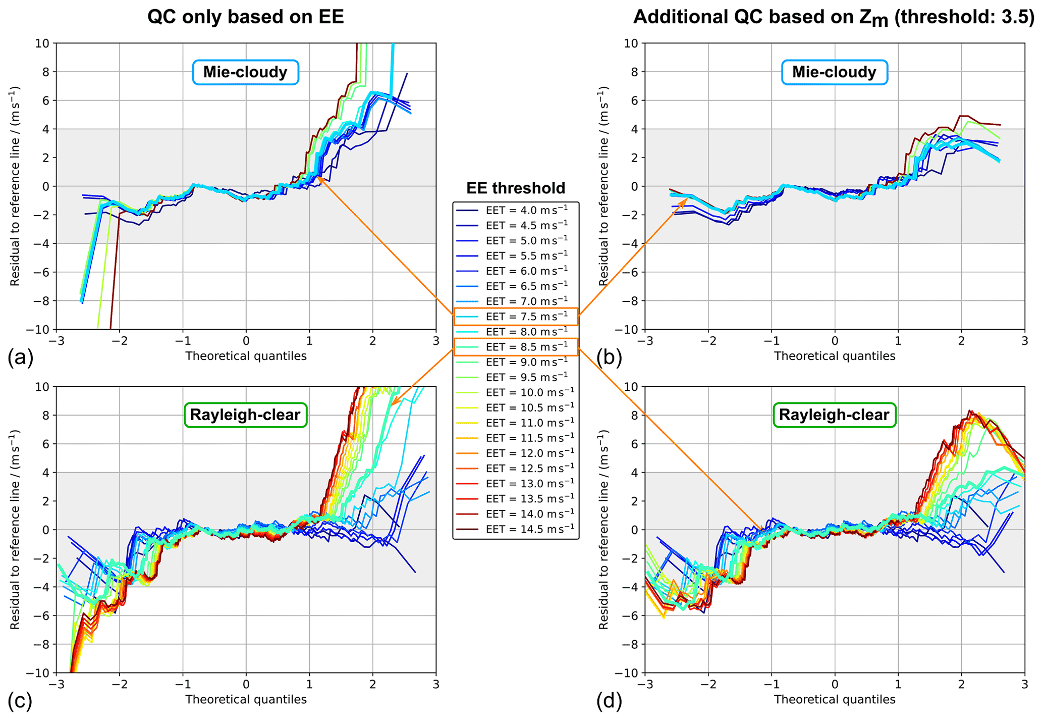
Figure 9Residual L2B Mie-cloudy (a, b) and Rayleigh-clear wind speed errors (c, d) after subtraction of the quartile reference line from the normal quantile plot based on the comparison to 2 µm DWL wind data from the AVATAR-T campaign. The residuals are calculated for different EE thresholds (EETs), as indicated by the colour scale. In panels (a) and (c), no additional outlier removal was applied, whereas the plots in panels (b) and (d) are obtained after additional QC, based on the modified Z score (|Zm|>3.5). The curves corresponding to the EE thresholds that are deemed reasonable to provide robust statistical results (Mie is 7.5 m s−1; Rayleigh is 8.5 m s−1) are plotted by thick lines.
The EE threshold for the Mie-cloudy winds was set to 7.5 m s−1, since this setting provides a large portion of valid wind results to be included in the statistics (88 %), while yielding very similar statistical results compared to smaller thresholds down to 5 m s−1, provided that additional filtering of outliers based on the modified Z score is applied. The suitability of the chosen EE thresholds is verified and visualized by normal quantile plots in Fig. 9, which depict the residuals to the reference line, as introduced in Sect. 3.4, that are, however, given in absolute wind speeds instead of quantiles, i.e. units of the standard deviation. The higher the EE threshold, the larger the departures from normality are, especially if no modified Z-score filter is applied (left column). When a two-step QC is used (right column), the Mie wind error exhibits rather small residuals which, however, exceed 4 m s−1 at EE thresholds beyond 8 m s−1. As for the Rayleigh channel, using a combination of EE threshold (8.5 m s−1) and a subsequent modified Z-score filter keeps the residuals below 4 m s−1 (grey-shaded area) within the first two theoretical quantiles, i.e. the 4σ range, including ≈95.5 % of the data that are left after applying the EE filter.
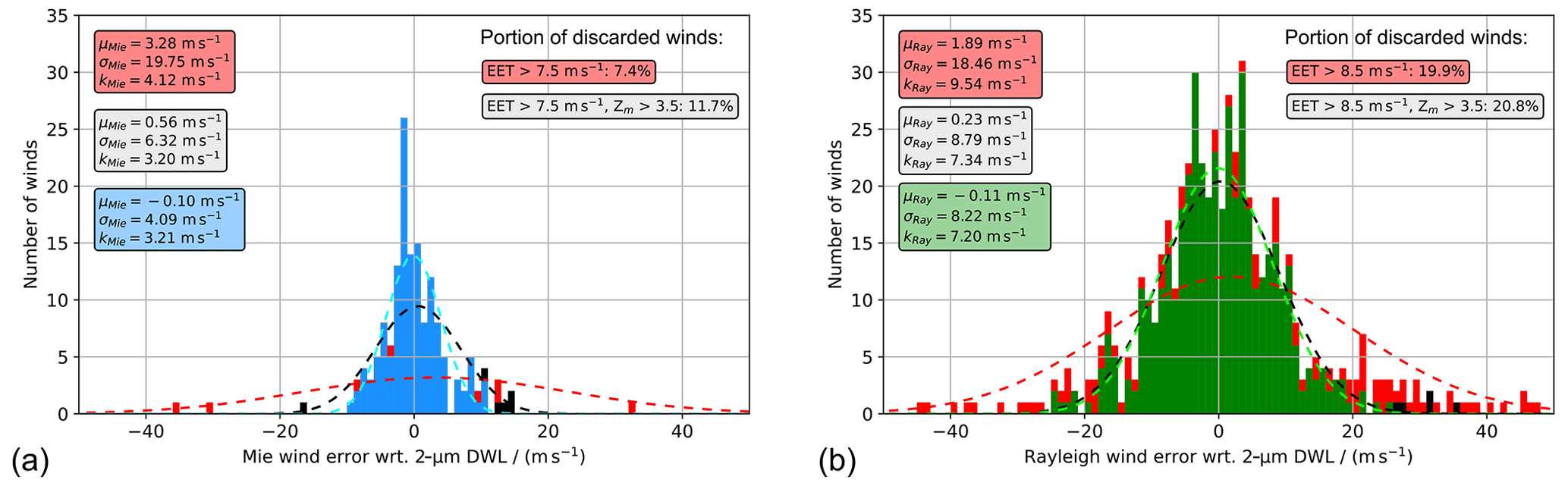
Figure 10Histograms of the Mie-cloudy (a) and Rayleigh-clear (b) wind errors with respect to the 2 µm DWL wind data acquired during the AVATAR-T campaign. The blue and green columns denote the histogram after discarding winds with EE >7.5 m s−1 (Mie) and EE >8.5 m s−1 (Rayleigh) and subsequent application of a QC based on the modified Z score (threshold of 3.5). The red columns indicate the winds that are filtered out by the EE threshold, while the black columns describe wind data that are additionally filtered out by the modified Z score. The statistical parameters given in the boxes refer to the three different subsets (red – all data; grey – EE filter only; blue/green – EE filter plus modified Z-score filter).
Finally, the PDFs of the Mie and Rayleigh wind errors are presented in Fig. 10, indicating those wind results that are filtered out by the EE threshold (red bars) and those that are additionally filtered out by the modified Z score (black bars). The statistical results that are provided in the boxes refer to the different subsets without QC (red), one-step QC, using solely the EE threshold (grey), and two-step QC, additionally applying the modified Z-score filter (blue/green). As discussed in Sect. 3, extreme gross errors in the Mie data drastically distort the statistics (μ=3.3 m s−1; σ≈20 m s−1) if they are not discarded from the dataset, while the EE threshold alone still retains a few positively biased outliers. The combined QC ensures robust statistics ( m s−1; σ=4.1 m s−1) based on 143 out of 162 Mie-cloudy wind results (88 %). The portion of valid Rayleigh winds that are included in the statistics after the two-step QC is slightly smaller but still close to 80 % (445 out of 563). Comparison of the histograms in Fig. 10b also illustrates how the QC increases the degree of normality by removing the thick tails of the Rayleigh-clear wind error distribution.
Table 3Statistical comparison of the Aeolus L2B Mie-cloudy and Rayleigh-clear winds against the 2 µm DWL winds for the first five underflights performed during the AVATAR-T campaign. The corresponding scatterplots and histograms are shown in Figs. 7 and 10, respectively. The statistics are derived after the adaptation of the 2 µm DWL wind data to the respective L2B measurement grids and applying an EE threshold filter (Mie is 7.5 m s−1; Rayleigh is 8.5 m s−1) and without and with an additional QC step based on the modified Z score (threshold is 3.5).
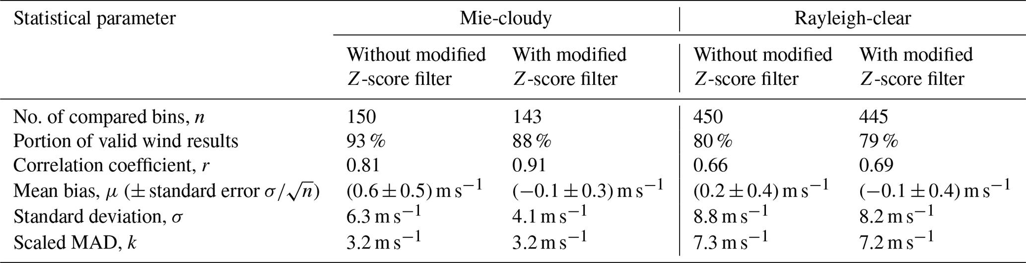
The statistical parameters derived from the 2 µm DWL validation study are summarized in Table 3. Comparing the results to those from the validation against the ECMWF model background data (Table 2), it is confirmed that both the Mie-cloudy and the Rayleigh-clear winds show a small systematic error of less than 0.3 m s−1 and thus fulfil the mission requirement, provided that the two-step QC is performed. The mean bias values with respect to the two reference datasets agree with each other within their respective standard errors (). However, the model comparison yields a larger random error in the Mie winds (σ=5.3 m s−1 compared to 4.1 m s−1), whereas the Rayleigh wind random error is determined to be smaller (7.8 m s−1 compared to 8.2 m s−1) than for the validation against the 2 µm DWL. These discrepancies can be partly explained by the fact that, unlike the ECMWF model background data, the 2 µm DWL wind data are only available in regions with significant particle backscatter from aerosols or clouds. Consequently, the Mie-cloudy wind results that overlap with the 2 µm DWL data are likely to be derived from high-SNR signals and are thus of high quality. In contrast, the Rayleigh-clear winds overlapping with the 2 µm DWL are expected to be noisier for the reasons stated above. However, when the model comparison discussed in Sect. 3 is restricted to those Aeolus wind results that were also validated by the 2 µm DWL (not shown), then the statistical results are not reproduced but rather lie between those illustrated in Figs. 6 and 8. This suggests that, in addition to the restricted overlap of the Aeolus data with the 2 µm DWL winds, spatial representativeness contributes to the deviations in the validation results. Moreover, discrepancies between the 2 µm DWL and model background wind data can result from model deficiencies that are caused by imperfect parameterization or too low resolution. Errors in the model background, i.e. before the assimilation of Aeolus winds, are found to be especially large in convective areas in the tropics, exceeding even 10 m s−1 on several occasions (Rennie et al., 2021). Finally, the QC for the model comparison did not use the EE and was only based on the modified Z score. However, if a two-step QC approach with similar EE thresholds as for the 2 µm DWL comparison was taken for the model comparison, then the statistical results would not differ much, as they rapidly converge when the EE threshold is relaxed beyond 8 m s−1 (see Fig. 6).
The present work underlines the necessity of a careful statistical analysis when assessing the Aeolus wind data quality and points out that QC of the wind results should not solely rely on static thresholds for the EE which is reported in the L2B product, as it has been highly variable over the course of the mission and depends on the geographical location. The EE of the Rayleigh-clear winds only considers the SNR, while other noise terms, e.g. related to the detector and read-out electronics, and the influence of temperature, pressure, or scattering ratio are not (yet) accounted for. The Mie-cloudy EE is calculated from the solution error covariance of the fit algorithm which determines the position of the Mie fringe. The signal distribution across the Mie detector is modified by the broadband Rayleigh signal and depends on the illumination conditions along the orbit. Together with the Lorentz fit routine, this gives rise to erroneous peak detection and thus non-physical wind speeds, especially in case of weak particulate backscatter signals, which are not adequately described by a sufficiently high EE. The resulting Mie gross errors are not evenly distributed but predominantly have a positive bias with respect to the reference wind data. Consequently, additional QC steps are required to filter out these outliers to ensure meaningful statistics in accordance with the definitions stated in Aeolus MRD. The modified Z score is introduced and demonstrated to be a valuable tool to identify and to sort out outliers stemming from non-Gaussian error sources, especially for small datasets, whereby a threshold ranging from 3.0 to 3.5 is recommended to obtain a wind error distribution with a high degree of normality. The latter can be evaluated by analysing normal quantile plots, whose interpretation is easier and less ambiguous than histograms, and this allows conclusions about the skewness and kurtosis of the distribution. In conclusion, a two-step QC based on the EE and modified Z score with individually derived thresholds is proposed to facilitate the comparability of validation results and to reduce the influence of the EE, which does not fully incorporate all relevant error sources for Aeolus.
The statistical methods were tested for the validation of Aeolus winds against ECMWF model background data and during the AVATAR-T campaign within the frame of the JATAC around the Cabo Verde archipelago in September 2021. Utilization of the modified Z score ensures that outliers, which are not assigned a large EE, are discarded from the analysis, while keeping a large portion of the original data. The approach, however, entails that non-physical wind results which, by chance, show small departures from the reference are retained as well. This circumstance is less critical for the Rayleigh-clear winds, as the fraction of outliers identified by the modified Z score is less than 5 %. The portion of Mie outliers is about twice as large, which means that the gross error requirement is not fulfilled.
A combined bar and line graph can be used to illustrate the dependence of the key statistical parameters (systematic and random error, portion of valid data, and outliers) on a chosen EE threshold. The graph not only provides the full picture with regard to the statistical analysis but also allows for the determination of suitable EE and modified Z score thresholds that account for the validating instrument's overlap and error characteristics with respect to Aeolus. In this manner, the results from diverse reference instruments or models spanning the same validation period can be compared to each other and are not biased by the varying influence of using a fixed EE threshold as sole QC criterion. The same holds true for the validation results from the same reference obtained in different phases of the Aeolus mission or in different geographical locations. Given the temporal and spatial variability in the EE, an adaption of the QC settings is necessary to ensure consistency and comparability.
The suggested two-step QC was also applied for the comparison of the Aeolus L2B winds against the 2 µm DWL wind data from the AVATAR-T campaign, using EE thresholds of 7.5 and 8.5 m s−1 for the Mie-cloudy and Rayleigh-clear winds, respectively, followed by a modified Z-score filter with a threshold of 3.5. This approach effectively removes all data outliers and yields near-Gaussian wind error distributions, while keeping the vast majority (80 %) of all valid Mie and Rayleigh winds in the statistical analysis. The systematic errors were determined to be below 0.3 m s−1 for both receiver channels, which agrees with the model comparison and confirms the conformity of the Aeolus winds with the systematic error mission requirement. The random errors of 4.1 m s−1 (Mie) and 8.2 m s−1 (Rayleigh) deviate from those derived from the validation against the model (5.3 and 7.8 m s−1). This is assumed to mainly stem from the incomplete data coverage of the 2 µm DWL, which tends to overlap with the Aeolus winds in regions where the Mie winds are of high quality, whereas the Rayleigh winds suffer from increased noise.
This work intends to provide a guideline on how to perform a rigorous QC when working with Aeolus wind data. The presented results have demonstrated that a careful QC scheme is crucial for rejecting gross errors and, in turn, for providing an accurate estimation of the wind data quality. The shown statistical methods form the basis for a standardization and objectification of the Aeolus wind validation and will be applied in forthcoming studies involving the DLR's wind lidar instruments. Furthermore, apart from the better comparability among different validation studies, the investigation fosters the analysis of the individual channel error characteristics and stimulates the refinement of the QC schemes that are currently used in the assimilation of Aeolus wind data into operational models. Both aspects are important to further improve the impact of the Aeolus products for NWP centres around the world.
In this context, it should be noted that the operational assimilation of Aeolus wind data at the ECMWF involves a multi-step QC scheme which also largely relies on the imperfect L2B EE. It comprises a first-guess check, which rejects observations with very large (O-B) departures (5σ), followed by the so-called variational QC (VarQC) method (Andersson and Järvinen, 1998). The VarQC assumes that the distribution of the normalized wind error, i.e. the (O-B) wind error divided by the assigned observation error, takes the form of a Gaussian function including an offset. The assigned observation error is proportional to the EE and additionally considers a representativeness error of 2 m s−1 for the Mie winds (Rennie et al., 2021). Finally, there is a blacklist in the ECMWF assimilation which removes Rayleigh winds below 850 hPa pressure altitude and Rayleigh-clear and Mie-cloudy winds with EE larger than 12 and ∼5 m s−1, respectively. The multi-step approach ensures the effective removal of the largest gross errors, but the VarQC assumption does not well represent the Aeolus normalized wind error distribution, especially for the Mie winds. In this regard, the use of the modified Z score may help to improve the performance of the QC in the Aeolus data assimilation.
The origin of the complex L2B wind error distributions is currently under investigation. Preliminary results show that outliers in the Rayleigh-clear dataset are not necessarily correlated with low signal levels, so that they exhibit low EE despite their large departures from the true wind speed. Here, a refinement of the EE calculation would improve the meaningfulness of the EE and thus the effectiveness of related QC schemes. In particular, the contribution of other noise sources, e.g. read-out noise, which increases with declining atmospheric return signal levels, should be properly accounted for. Additionally, the consideration of terms that describe the influence of temperature, pressure, and scattering ratio on the Rayleigh response, which were originally foreseen to be included in the computation of the EE, would further reduce the risk of underestimating the Rayleigh-clear EE. Regarding the Mie-cloudy winds, current investigations aim at identifying the causes of the strongly asymmetric wind error distribution. Apart from orbital variations in the telescope illumination, the signal distribution across the Mie detector is also influenced by imperfections of the Fizeau interferometer, which manifest in a partially distorted Mie fringe. The latter is found to result in large Mie wind biases in the A2D data in the case of strong backscatter gradients, e.g. at cloud boundaries (Lux et al., 2022). A similar error source is possible for the Aeolus Mie channel, potentially causing large wind errors despite high SNR and, hence, low EE. Improvement in the Mie EE is expected from a refinement of the threshold settings and the fit function, e.g. Voigt instead of Lorentzian line shape, used within the Mie Core algorithm, which is supposed to reduce the portion of gross errors to less than 5 % and to prevent gross errors outside of the 6σ range (up to ±15 m s−1), as specified in the mission requirements.
The presented work includes data of the Aeolus mission which is part of the European Space Agency (ESA) Earth Explorer Programme. This includes the reprocessed L2B wind product (Baseline 12; de Kloe et al., 2022; https://earth.esa.int/eogateway/documents/20142/37627/Aeolus-L2B-2C-Input-Output-DD-ICD.pdf, last access: 13 June 2022) for the period of the AVATAR-T campaign (from 6 through 28 September 2021) that is publicly available and can be accessed via the ESA Aeolus Online Dissemination System (https://aeolus-ds.eo.esa.int/oads/access/collection/_L2C_Wind_Products, last access: 13 June 2022; European Space Agency, 2022). The processor development, improvement, and product reprocessing preparation have been performed by the Aeolus DISC (Data, Innovation and Science Cluster), which involves DLR, DoRIT, TROPOS, ECMWF, KNMI, CNRS, S&T, ABB, and Serco, in close cooperation with the Aeolus PDGS (Payload Data Ground Segment). The 2 µm DWL data used in this paper can be provided upon reasonable request to Benjamin Witschas (benjamin.witschas@dlr.de).
OL, BW, AG, CL, and OR performed the studies. CL was the principal investigator of the AVATAR-T campaign. AG, FW, and UM supported the data analysis. BW and SR carried out the 2 µm DWL measurements and processed the 2 µm DWL data. CL, OR, AG, and AS conducted the flight planning. The paper was written by OL, with contributions from all co-authors.
The contact author has declared that none of the authors has any competing interests.
Publisher's note: Copernicus Publications remains neutral with regard to jurisdictional claims in published maps and institutional affiliations.
This article is part of the special issue “Aeolus data and their application (AMT/ACP/WCD inter-journal SI)”. It is not associated with a conference.
The timeline of the atmospheric signal levels presented in Fig. 1 was kindly provided by Karsten Schmidt. We thank Michael Rennie (ECMWF) and Jos de Kloe (KNMI), for providing insights to the calculation and temporal evolution of the Aeolus L2B estimated error and to the QC schemes that are used in the Aeolus data assimilation at ECMWF. We are also grateful to our ESA colleagues Thorsten Fehr (Aeolus scientific campaign coordinator) and Jonas von Bismarck (Aeolus data quality manager), for their support of the study. Finally, we would like to thank the DLR flight experiments department, for the realization of the AVATAR-T airborne campaign despite the obstacles posed by the COVID-19 pandemic.
The AVATAR-T campaign was supported by the European Space Agency (grant no. 4000129946/20/NL/IA). Parts of this research have been supported by the German Federal Ministry for Economic Affairs and Energy (BMWi; grant no. 50EE1721A).
The article processing charges for this open-access publication were covered by the German Aerospace Center (DLR).
This paper was edited by Ad Stoffelen and reviewed by three anonymous referees.
Andersson, E.: Statement of Guidance for Global Numerical Weather Prediction (NWP), World Meteorological Organisation, https://docplayer.net/194586713-Statement-of-guidance-for-global-numerical-weatherprediction-nwp.html (last access: 19 May 2022), 2018.
Andersson, E. and Järvinen, H.: Variational quality control, Technical Memorandum, ECMWF, https://doi.org/10.21957/lqz2wn16g, 1998.
Baars, H., Herzog, A., Heese, B., Ohneiser, K., Hanbuch, K., Hofer, J., Yin, Z., Engelmann, R., and Wandinger, U.: Validation of Aeolus wind products above the Atlantic Ocean, Atmos. Meas. Tech., 13, 6007–6024, https://doi.org/10.5194/amt-13-6007-2020, 2020.
Bedka, K. M., Nehrir, A. R., Kavaya, M., Barton-Grimley, R., Beaubien, M., Carroll, B., Collins, J., Cooney, J., Emmitt, G. D., Greco, S., Kooi, S., Lee, T., Liu, Z., Rodier, S., and Skofronick-Jackson, G.: Airborne lidar observations of wind, water vapor, and aerosol profiles during the NASA Aeolus calibration and validation (Cal/Val) test flight campaign, Atmos. Meas. Tech., 14, 4305–4334, https://doi.org/10.5194/amt-14-4305-2021, 2021.
Chambers, J. M., Cleveland, W. S., Kleiner, B., and Tukey, P. A. (Eds.): Graphical Methods for Data Analysis, Chapman and Hall/CRC, 1983.
Chanin, M. L., Garnier, A., Hauchecorne, A., and Porteneuve, J.: A Doppler lidar for measuring winds in the middle atmosphere, Geophys. Res. Lett., 16, 1273–1276, https://doi.org/10.1029/GL016i011p01273, 1989.
Chen, S., Cao, R., Xie, Y., Zhang, Y., Tan, W., Chen, H., Guo, P., and Zhao, P.: Study of the seasonal variation in Aeolus wind product performance over China using ERA5 and radiosonde data, Atmos. Chem. Phys., 21, 11489–11504, https://doi.org/10.5194/acp-21-11489-2021, 2021.
Chou, C.-C., Kushner, P. J., Laroche, S., Mariani, Z., Rodriguez, P., Melo, S., and Fletcher, C. G.: Validation of the Aeolus Level-2B wind product over Northern Canada and the Arctic, Atmos. Meas. Tech., 15, 4443–4461, https://doi.org/10.5194/amt-15-4443-2022, 2022.
Cress, A. and Martin, A.: Validation and impact assessment of Aeolus observations in the DWD modelling system, Taormina, Italy, 28 March–1 April 2022, https://www.aeolus3years.org/detailed-agenda, last access: 19 May 2022.
Dabas, A., Denneulin, M. L., Flamant, P., Loth, C., Garnier, A., and Dolfi-Bouteyre, A.: Correcting winds measured with a Rayleigh Doppler lidar from pressure and temperature effects, Tellus A, 60, 206–215, https://doi.org/10.1111/j.1600-0870.2007.00284.x, 2008.
de Kloe, J., Stoffelen, A., Tan, D., Andersson, E., Rennie, M., Dabas, A., Poli, P., and Huber, D.: ADM-Aeolus Level-2B/2C Processor Input/Output Data Definitions Interface Control Document, AED-SD-ECMWF-L2B-037, v. 3.70, 122 pp., https://earth.esa.int/eogateway/documents/20142/37627/Aeolus-L2B-2C-Input-Output-DD-ICD.pdf, last access: 13 June 2022.
European Space Agency (ESA): ADM-Aeolus Science Report, ESA SP-1311, 121 pp., European Space Agency, https://esamultimedia.esa.int/multimedia/publications/SP-1311/SP-1311.pdf (last access: 19 May 2022), 2008.
European Space Agency (ESA): ADM-Aeolus Mission Requirements Document, ESA EOP-SM/2047, 57 pp., European Space Agency, https://earth.esa.int/eogateway/documents/20142/1564626/Aeolus-Mission-Requirements.pdf (last access: 20 May 2022), 2016.
European Space Agency (ESA): L2C assimilated wind products, https://aeolus-ds.eo.esa.int/oads/access/collection/L2C_Wind_Products, last access: 13 June 2022.
Fehr, T.: The Joint Aeolus Tropical Atlantic Campaign 2021, Taormina, Italy, 28 March–1 April 2022, https://www.aeolus3years.org/detailed-agenda, last access: 19 May 2022.
Flesia, C. and Korb, C. L.: Theory of the double-edge molecular technique for Doppler lidar wind measurement, Appl. Optics, 38, 432, https://doi.org/10.1364/AO.38.000432, 1999.
Garnier, A. and Chanin, M. L.: Description of a Doppler Rayleigh LIDAR for measuring winds in the middle atmosphere, Appl. Phys. B, 55, 35–40, https://doi.org/10.1007/BF00348610, 1992.
Gentry, B. M., Chen, H., and Li, S. X.: Wind measurements with 355-nm molecular Doppler lidar, Opt. Lett., 25, 1231–1233, https://doi.org/10.1364/OL.25.001231, 2000.
Halloran, G.: UK Met Office NWP impact of Aeolus winds, Taormina, Italy, 28 March–1 April 2022, https://www.aeolus3years.org/detailed-agenda, last access: 19 May 2022.
Iglewicz, B. and Hoaglin, D. C.: How to Detect and Handle Outliers, American Society for Quality Control, Statistics Division, vol. 16, ASQ Quality Press, 1993.
Iwai, H., Aoki, M., Oshiro, M., and Ishii, S.: Validation of Aeolus Level 2B wind products using wind profilers, ground-based Doppler wind lidars, and radiosondes in Japan, Atmos. Meas. Tech., 14, 7255–7275, https://doi.org/10.5194/amt-14-7255-2021, 2021.
Kanitz, T., Lochard, J., Marshall, J., McGoldrick, P., Lecrenier, O., Bravetti, P., Reitebuch, O., Rennie, M., Wernham, D., and Elfving, A.: Aeolus First Light – First Glimpse, Proc. SPIE, 11180, 111801R, https://doi.org/10.1117/12.2535982, 2019.
Kanitz, T., Wernham, D., Alvarez, E., Tzeremes, G., Parrinello, T., Marshall, J., Brewster, J., Lecrenier, O., Schillinger, M., de Sanctis, V., D'Ottavi, A., Reitebuch, O., Weiler, F., Lux, O., Rennie, M., and Isaksen, L.: Aeolus – ESA'S Wind Lidar Mission, A Brief Status, in: 2020 IEEE International Geoscience and Remote Sensing Symposium, Waikoloa, USA, 26 September–2 October 2020, 3463–3466, 2020.
Liu, B., Guo, J., Gong, W., Zhang, Y., Shi, L., Ma, Y., Li, J., Guo, X., Stoffelen, A., de Leeuw, G., and Xu, X.: Intercomparison of wind observations from ESA's satellite mission Aeolus, ERA5 reanalysis and radiosonde over China, Atmos. Meas. Tech. Discuss. [preprint], https://doi.org/10.5194/amt-2022-26, 2022.
Lorenc, A. C. and Hammon, O.: Objective quality control of observations using Bayesian methods. Theory, and a practical implementation, Q. J. Roy. Meteor. Soc., 114, 515–543, https://doi.org/10.1002/qj.49711448012, 1988.
Lux, O., Lemmerz, C., Weiler, F., Marksteiner, U., Witschas, B., Rahm, S., Schäfler, A., and Reitebuch, O.: Airborne wind lidar observations over the North Atlantic in 2016 for the pre-launch validation of the satellite mission Aeolus, Atmos. Meas. Tech., 11, 3297–3322, https://doi.org/10.5194/amt-11-3297-2018, 2018.
Lux, O., Lemmerz, C., Weiler, F., Marksteiner, U., Witschas, B., Rahm, S., Geiß, A., and Reitebuch, O.: Intercomparison of wind observations from the European Space Agency's Aeolus satellite mission and the ALADIN Airborne Demonstrator, Atmos. Meas. Tech., 13, 2075–2097, https://doi.org/10.5194/amt-13-2075-2020, 2020a.
Lux, O., Wernham, D., Bravetti, P., McGoldrick, P., Lecrenier, O., Riede, W., D'Ottavi, A., Sanctis, V. de, Schillinger, M., Lochard, J., Marshall, J., Lemmerz, C., Weiler, F., Mondin, L., Ciapponi, A., Kanitz, T., Elfving, A., Parrinello, T., and Reitebuch, O.: High-power and frequency-stable ultraviolet laser performance in space for the wind lidar on Aeolus, Opt. Lett., 45, 1443–1446, https://doi.org/10.1364/OL.387728, 2020b.
Lux, O., Lemmerz, C., Weiler, F., Kanitz, T., Wernham, D., Rodrigues, G., Hyslop, A., Lecrenier, O., McGoldrick, P., Fabre, F., Bravetti, P., Parrinello, T., and Reitebuch, O.: ALADIN laser frequency stability and its impact on the Aeolus wind error, Atmos. Meas. Tech., 14, 6305–6333, https://doi.org/10.5194/amt-14-6305-2021, 2021.
Lux, O., Lemmerz, C., Weiler, F., Marksteiner, U., Witschas, B., Rahm, S., Geiß, A., Schäfler, A., and Reitebuch, O.: Retrieval improvements for the ALADIN Airborne Demonstrator in support of the Aeolus wind product validation, Atmos. Meas. Tech., 15, 1303–1331, https://doi.org/10.5194/amt-15-1303-2022, 2022.
Marksteiner, U.: Airborne Wind Lidar Observations for the Validation of the ADM-Aeolus Instrument, PhD thesis, Technische Universität München, 180 pp., https://pdfs.semanticscholar.org/6e2a/9435e63122a5bfce5fdbe0b881c76fd79_62f.pdf (last access: 2 June 2022), 2013.
Marseille, G.-J., Kloe, J., Marksteiner, U., Reitebuch, O., Rennie, M., and Haan, S.: NWP calibration applied to Aeolus Mie channel winds, Q. J. Roy. Meteor. Soc., 148, 1020–1034, https://doi.org/10.1002/qj.4244, 2022.
Martin, A., Weissmann, M., Reitebuch, O., Rennie, M., Geiß, A., and Cress, A.: Validation of Aeolus winds using radiosonde observations and numerical weather prediction model equivalents, Atmos. Meas. Tech., 14, 2167–2183, https://doi.org/10.5194/amt-14-2167-2021, 2021.
McKay, J. A.: Assessment of a multibeam Fizeau wedge interferometer for Doppler wind lidar, Appl. Optics, 41, 1760, https://doi.org/10.1364/AO.41.001760, 2002.
Nelder, J. A. and Mead, R.: A Simplex Method for Function Minimization, The Computer Journal, 7, 308–313, https://doi.org/10.1093/comjnl/7.4.308, 1965.
Parrinello, T.: Aeolus: 3 Years in Space. Status and Future Challenges, Aeolus 3rd Anniversary Conference, Taormina, Italy, 28 March–1 April 2022, https://www.aeolus3years.org/detailed-agenda, last access: 19 May 2022.
Reitebuch, O.: The Spaceborne Wind Lidar Mission ADM-Aeolus, in: Atmospheric physics: Background, methods, trends, edited by: Schumann, U., Research Topics in Aerospace, Springer, Berlin, London, 815–827, 2012.
Reitebuch, O.: Contributions from the DISC to accomplish the Aeolus mission objectives, Taormina, Italy, 28 March–1 April 2022, https://www.aeolus3years.org/detailed-agenda, last access: 23 May 2022.
Reitebuch, O., Huber, D., and Nikolaus, I.: “ADM-Aeolus Algorithm Theoretical Basis Document (ATBD) Level-1B Products”, AE-RP-DLR-L1B-001, vol. 4.4, 117 pp., https://earth.esa.int/eogateway/documents/20142/37627/Aeolus-L1B-Algorithm-ATBD.pdf (last access: 13 May 2022), 2018.
Reitebuch, O., Lemmerz, C., Lux, O., Marksteiner, U., Rahm, S., Weiler, F., Witschas, B., Meringer, M., Schmidt, K., Huber, D., Nikolaus, I., Geiss, A., Vaughan, M., Dabas, A., Flament, T., Stieglitz, H., Isaksen, L., Rennie, M., Kloe, J. D., Marseille, G.-J., Stoffelen, A., Wernham, D., Kanitz, T., Straume, A.-G., Fehr, T., Bismarck, J. von, Floberghagen, R., and Parrinello, T.: Initial Assessment of the Performance of the First Wind Lidar in Space on Aeolus, EPJ Web Conf., 237, 1010, https://doi.org/10.1051/epjconf/202023701010, 2020.
Rennie, M. and Isaksen, L.: The NWP impact of Aeolus Level-2B winds at ECMWF, Technical Memorandum ECMWF, https://www.ecmwf.int/sites/default/files/elibrary/2020/19538-nwp-impact-aeolus-level-2b-winds-ecmwf.pdf (last access: 1 August 2022), 2020.
Rennie, M., Tan, D., Andersson, E., Poli, P., Dabas, A., De Kloe, J., Marseille, G.-J., and Stoffelen, A.: Aeolus Level-2B Algorithm Theoretical Basis Document (Mathematical Description of the Aeolus L2B Processor), AED-SD-ECMWF-L2B-038, vol. 3.4, 124 pp., https://earth.esa.int/eogateway/missions/aeolus/data (last access: 13 May 2022), 2020.
Rennie, M. P., Isaksen, L., Weiler, F., Kloe, J., Kanitz, T., and Reitebuch, O.: The impact of Aeolus wind retrievals in ECMWF global weather forecasts, Q. J. Roy. Meteor. Soc., 147, 3555–3586, https://doi.org/10.1002/qj.4142, 2021.
Sandbhor, S. and Chaphalkar, N. B.: Impact of Outlier Detection on Neural Networks Based Property Value Prediction, in: Information Systems Design and Intelligent Applications, edited by: Satapathy, S. C., Bhateja, V., Somanah, R., Yang, X.-S., and Senkerik, R., Springer Singapore, Singapore, 481–495, https://doi.org/10.1007/978-981-13-3329-3_45, 2019.
Shiffler, R. E.: Maximum Z Scores and Outliers, The American Statistician, 42, 79–80, https://doi.org/10.1080/00031305.1988.10475530, 1988.
Stoffelen, A., Pailleux, J., Källen, E., Vaughan, M., Isaksen, L., Flamant, P., Wergen, W., Andersson, E., Schyberg, H., Culoma, A., Meynart, R., Endemann, M., and Ingmann, P.: The Atmospheric Dynamics Mission for Global Wind Field Measurement, B. Am. Meteorol. Soc., 86, 73–87, https://doi.org/10.1175/BAMS-86-1-73, 2005.
Stoffelen, A., Benedetti, A., Borde, R., Dabas, A., Flamant, P., Forsythe, M., Hardesty, M., Isaksen, L., Källén, E., Körnich, H., Lee, T., Reitebuch, O., Rennie, M., Riishøjgaard, L.-P., Schyberg, H., Straume, A. G., and Vaughan, M.: Wind Profile Satellite Observation Requirements and Capabilities, B. Am. Meteorol. Soc., 101, E2005–E2021, https://doi.org/10.1175/BAMS-D-18-0202.1, 2020.
Straume, A. G., Rennie, M., Isaksen, L., Kloe, J. de, Marseille, G.-J., Stoffelen, A., Flament, T., Stieglitz, H., Dabas, A., Huber, D., Reitebuch, O., Lemmerz, C., Lux, O., Marksteiner, U., Weiler, F., Witschas, B., Meringer, M., Schmidt, K., Nikolaus, I., Geiss, A., Flamant, P., Kanitz, T., Wernham, D., Bismarck, J. von, Bley, S., Fehr, T., Floberghagen, R., and Parinello, T.: ESA's Space-Based Doppler Wind Lidar Mission Aeolus – First Wind and Aerosol Product Assessment Results, EPJ Web Conf., 237, 1007, https://doi.org/10.1051/epjconf/202023701007, 2020.
Tan, D. G. H., Andersson, E., Kloe, J. D., Marseille, G.-J., Stoffelen, A., Poli, P., Denneulin, M.-L., Dabas, A., Huber, D., Reitebuch, O., FLAMANT, P., Le Rille, O., and Nett, H.: The ADM-Aeolus wind retrieval algorithms, Tellus A, 60, 191–205, https://doi.org/10.1111/j.1600-0870.2007.00285.x, 2008.
Tripathy, S. S.: Comparison of Statistical Methods for Outlier Detection in Proficiency Testing Data on Analysis of Lead in Aqueous Solution, AJTAS, 2, 233, https://doi.org/10.11648/j.ajtas.20130206.21, 2013.
Weiler, F., Kanitz, T., Wernham, D., Rennie, M., Huber, D., Schillinger, M., Saint-Pe, O., Bell, R., Parrinello, T., and Reitebuch, O.: Characterization of dark current signal measurements of the ACCDs used on board the Aeolus satellite, Atmos. Meas. Tech., 14, 5153–5177, https://doi.org/10.5194/amt-14-5153-2021, 2021a.
Weiler, F., Rennie, M., Kanitz, T., Isaksen, L., Checa, E., de Kloe, J., Okunde, N., and Reitebuch, O.: Correction of wind bias for the lidar on board Aeolus using telescope temperatures, Atmos. Meas. Tech., 14, 7167–7185, https://doi.org/10.5194/amt-14-7167-2021, 2021b.
Weissmann, M., Busen, R., Dörnbrack, A., Rahm, S., and Reitebuch, O.: Targeted Observations with an Airborne Wind Lidar, J. Atmos. Ocean. Tech., 22, 1706–1719, https://doi.org/10.1175/JTECH1801.1, 2005.
Witschas, B., Rahm, S., Dörnbrack, A., Wagner, J., and Rapp, M.: Airborne Wind Lidar Measurements of Vertical and Horizontal Winds for the Investigation of Orographically Induced Gravity Waves, J. Atmos. Ocean. Tech., 34, 1371–1386, https://doi.org/10.1175/JTECH-D-17-0021.1, 2017.
Witschas, B., Lemmerz, C., Geiß, A., Lux, O., Marksteiner, U., Rahm, S., Reitebuch, O., and Weiler, F.: First validation of Aeolus wind observations by airborne Doppler wind lidar measurements, Atmos. Meas. Tech., 13, 2381–2396, https://doi.org/10.5194/amt-13-2381-2020, 2020.
Witschas, B., Lemmerz, C., Geiß, A., Lux, O., Marksteiner, U., Rahm, S., Reitebuch, O., Schäfler, A., and Weiler, F.: Validation of the Aeolus L2B wind product with airborne wind lidar measurements in the polar North Atlantic region and in the tropics, Atmos. Meas. Tech. Discuss. [preprint], https://doi.org/10.5194/amt-2022-233, in review, 2022a.
Witschas, B., Lemmerz, C., Lux, O., Marksteiner, U., Reitebuch, O., Weiler, F., Fabre, F., Dabas, A., Flament, T., Huber, D., and Vaughan, M.: Spectral performance analysis of the Aeolus Fabry–Pérot and Fizeau interferometers during the first years of operation, Atmos. Meas. Tech., 15, 1465–1489, https://doi.org/10.5194/amt-15-1465-2022, 2022b.
Wu, S., Sun, K., Dai, G., Wang, X., Liu, X., Liu, B., Song, X., Reitebuch, O., Li, R., Yin, J., and Wang, X.: Inter-comparison of wind measurements in the atmospheric boundary layer and the lower troposphere with Aeolus and a ground-based coherent Doppler lidar network over China, Atmos. Meas. Tech., 15, 131–148, https://doi.org/10.5194/amt-15-131-2022, 2022.
Zuo, H., Hasager, C. B., Karagali, I., Stoffelen, A., Marseille, G.-J., and de Kloe, J.: Evaluation of Aeolus L2B wind product with wind profiling radar measurements and numerical weather prediction model equivalents over Australia, Atmos. Meas. Tech., 15, 4107–4124, https://doi.org/10.5194/amt-15-4107-2022, 2022.
The (standard) Z score, which is also often used for outlier detection, is defined as the distance from the mean in units of the standard deviation. A common approach is then to label observations with a Z score greater than 3 (in absolute values) as an outlier. However, the use of the Z score can be misleading due to the fact that μ and σ are affected by outliers themselves. Moreover, for a given sample size n, the maximum Z score is at most (Shiffler, 1988), so that Z is always below 3 for n=10. Therefore, it is not considered appropriate for outlier detection, particularly for small datasets.
- Abstract
- Introduction
- Datasets and the L2B estimated error
- QC methods for the L2B error assessment
- Aeolus validation against 2 µm DWL winds from AVATAR-T
- Discussion and summary
- Conclusions and outlook
- Data availability
- Author contributions
- Competing interests
- Disclaimer
- Special issue statement
- Acknowledgements
- Financial support
- Review statement
- References