the Creative Commons Attribution 4.0 License.
the Creative Commons Attribution 4.0 License.
 | 02 Nov 2022
HRLT: a high-resolution (1 d, 1 km) and long-term (1961–2019) gridded dataset for surface temperature and precipitation across China
Rongzhu Qin
Zeyu Zhao
Jia Xu
Jian-Sheng Ye
Feng-Min Li
Feng Zhang
Accurate long-term temperature and precipitation estimates at high spatial and temporal resolutions are vital for a wide variety of climatological studies. We have produced a new, publicly available, daily, gridded maximum temperature, minimum temperature, and precipitation dataset for China with a high spatial resolution of 1 km that covers a long-term period (1961 to 2019). It has been named the HRLT, and the dataset is publicly available at https://doi.org/10.1594/PANGAEA.941329 (Qin and Zhang, 2022). In this study, the daily gridded data were interpolated using comprehensive statistical analyses, which included machine learning methods, the generalized additive model, and thin plate splines. It was based on the 0.5∘ × 0.5∘ gridded dataset from the China Meteorological Administration, together with covariates for elevation, aspect, slope, topographic wetness index, latitude, and longitude. The accuracy of the HRLT daily dataset was assessed using observation data from meteorological stations across China. The maximum and minimum temperature estimates were more accurate than the precipitation estimates. For maximum temperature, the mean absolute error (MAE), root mean square error (RMSE), Pearson's correlation coefficient (Cor), coefficient of determination after adjustment (R2), and Nash–Sutcliffe modeling efficiency (NSE) were 1.07 ∘C, 1.62 ∘C, 0.99, 0.98, and 0.98, respectively. For minimum temperature, the MAE, RMSE, Cor, R2, and NSE were 1.08 ∘C, 1.53 ∘C, 0.99, 0.99, and 0.99, respectively. For precipitation, the MAE, RMSE, Cor, R2, and NSE were 1.30 mm, 4.78 mm, 0.84, 0.71, and 0.70, respectively. The accuracy of the HRLT was compared to those of three other existing datasets, and its accuracy was either greater than the others, especially for precipitation, or comparable in accuracy, but with higher spatial resolution or over a longer time period. In summary, the HRLT dataset, which has a high spatial resolution, covers a longer period of time and has reliable accuracy.
- Article
(12626 KB) - Full-text XML
- BibTeX
- EndNote


Climate change has led to an increase in the frequency and severity of extreme temperature and precipitation events (Myhre et al., 2019), and these events have affected vegetation growth (Xu et al., 2019), especially crop growth (Rao et al., 2015; Y. Li et al., 2019; Lu et al., 2018; Lobell et al., 2011; Lesk et al., 2016). Thus, long-term and accurate daily maximum temperature, minimum temperature, and precipitation data are important when attempting to reveal the mechanism underlying the effects of extreme climate on plants, for predicting disasters (such as drought, frost, and floods), and for agricultural and forestry management. Although the meteorological observation network makes better use of the data from meteorological stations (Merino et al., 2014; Yang et al., 2014), there is a tradeoff between large spatial scale and the high density of stations in the meteorological observation network. Moreover, the installation and maintenance of meteorological stations are challenging in harsh areas (Hartl et al., 2020). Daily and gridded meteorological datasets are also essential inputs for many models related to terrestrial, hydrological, and ecological systems (Iizumi et al., 2017; Wang et al., 2018; Zhang et al., 2018; Lee et al., 2019). High-resolution, long-term, and accurate gridded datasets can help improve the performance of these models.
Researchers have previously used interpolation methods, such as inverse distance weighting, kriging, and regression analysis, to produce gridded meteorological data (Brinckmann et al., 2016; Herrera et al., 2019; Schamm et al., 2014). However, the accuracy of these interpolation results is limited by the density of the meteorological stations. In recent years, artificial intelligence has been gradually and widely applied to meteorological data estimation, as have machine learning methods such as random forest (Chen et al., 2021; Sekulić et al., 2021), artificial neural networks (Sadeghi et al., 2021), and support vector machines (He et al., 2021) have been gradually and widely applied to meteorological data estimation. Therefore, comprehensive statistical analyses using machine learning and traditional interpolation, such as thin-plate-smoothing splines, are feasible and reliable methods that can be used to estimate meteorological data.
At present, only a few research institutes in China are developing meteorological datasets for temperature and precipitation with high spatial and temporal resolutions. Among them, Beijing Normal University has produced meteorological datasets for 1958–2010 with a resolution of 1 km, but the latest data are not available (Li et al., 2014). The China Meteorological Administration is also developing the CMA Land Data Assimilation System product (Shi et al., 2011), and Tsinghua University has published a driving dataset from 1979 to 2018 with a resolution of 0.1∘ over China (He et al., 2020).
We present a new high-resolution daily gridded maximum temperature, minimum temperature, and precipitation dataset for China (HRLT) with a spatial resolution of 1×1 km for the period 1961 to 2019. We created the HRLT dataset using comprehensive statistical analyses, which included machine learning, the generalized additive model, and thin plate splines. It uses the 0.5∘ × 0.5∘ gridded dataset from the China Meteorological Administration (CMA) as input data together with other covariates, including elevation, aspect, slope, topographic wetness index (TWI), latitude, and longitude. The dataset was created in three steps: (1) preparation of input data and covariates; (2) the creation of the gridded dataset using comprehensive statistical analyses; and (3) an evaluation of the accuracy of the gridded dataset and an accuracy comparison with three other existing products that use meteorological station data.
2.1 The CMA dataset and meteorological station data
The CMA dataset, which includes the daily surface temperature 0.5∘ × 0.5∘ gridded dataset and the daily precipitation 0.5∘ × 0.5∘ gridded dataset for China (V2.0) (https://data.cma.cn/, last access: 15 September 2022), was obtained from the China Meteorological Data Service Centre and was used as the basic input data. The researchers also reported a daily precipitation 0.5∘ × 0.5∘ gridded dataset for 1961–2010 from the CAM dataset (Zhao and Zhu, 2015). The daily dataset of surface climatological data for China (V3.0) (https://data.cma.cn/, last access: 15 September 2022), which includes 699 meteorological stations, was also obtained from the China Meteorological Data Service Centre and was used to evaluate the new dataset (Fig. 1).
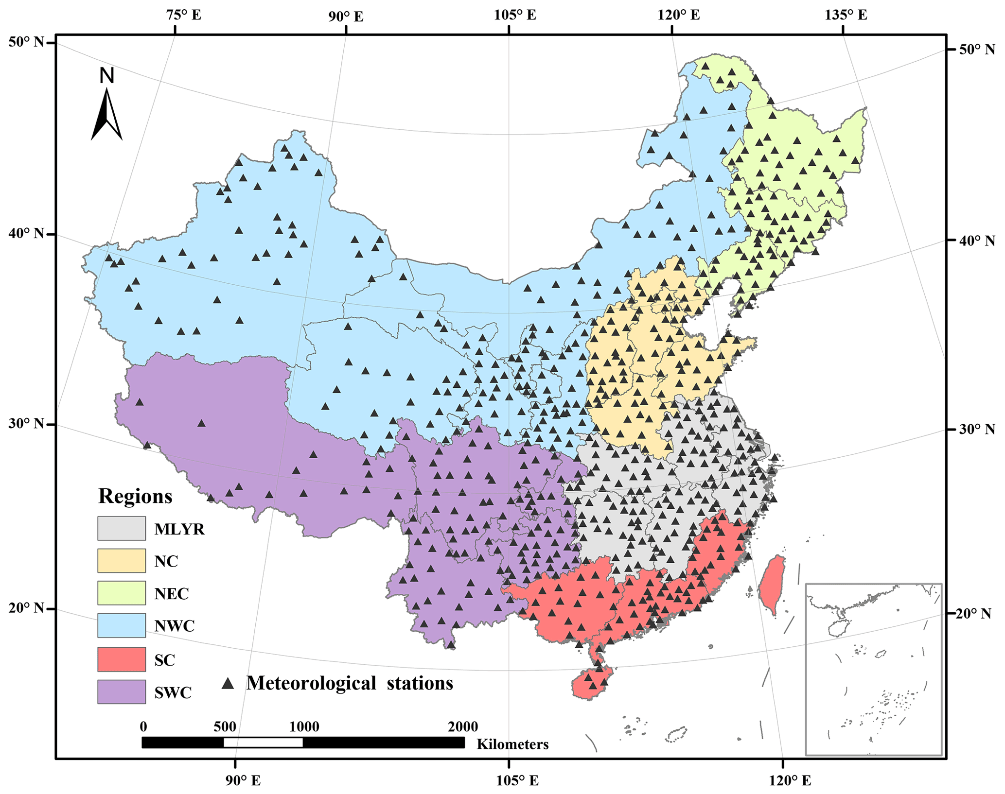
Figure 1Regions and spatial distribution of the meteorological stations in China. MLYR, NC, NEC, NWC, SC, and SWC are the middle and lower reaches of the Yangtze River, North China, Northeast China, Northwest China, South China, and Southwest China, respectively. Note: meteorological station data were missing for Taiwan Province.
2.2 Topographic data
The basic topographic data, including elevation, flow direction, and flow accumulation with 30 s (approximately 1 km) resolution, were obtained from the HydroSHEDS database. More detailed information can be found at these links: http://www.worldwildlife.org/hydrosheds (last access: 15 September 2022) (for general information) and http://hydrosheds.cr.usgs.gov (last access: 15 September 2022) (for downloading data and for technical information). The “Aspect” and “Slope” options of the Spatial Analyst Tools in ArcGIS10.6 were used to calculate the aspect and slope. The specific catchment area (SCA) was calculated based on the flow direction and flow accumulation.
The TWI is formulated as follows:
where TWI and SCA are the topographic wetness index and specific catchment area, respectively.
2.3 Other datasets
We used observed data from meteorological stations (Fig. 1) to evaluate our dataset and the three existing daily datasets, and then the accuracies of the three existing daily datasets were compared to that of our dataset. The China Meteorological Administration Land Data Assimilation System (CLDAS) version 2 dataset was provided by the China Meteorological Data Service Centre (https://data.cma.cn/, last access: 15 September 2022) for 2017 to 2019 with 0.0625∘ (approximately 7.5 km) spatial resolution and 1 d temporal resolution. The China Meteorological Forcing Dataset (CMFD) (He et al., 2020; Yang and He, 2019) was obtained from the National Tibetan Plateau Third Pole Environment Data Center (https://data.tpdc.ac.cn/, last access: 15 September 2022) for 1979 to 2018 with a spatial resolution of 0.1∘ (approximately 12 km) and a temporal resolution of 1 d. The historical dataset relating to the Inter-Sectoral Impact Model Intercomparison Project (ISIMIP3a) was obtained from the web (https://data.isimip.org/, last access: 15 September 2022) for 1961 to 2016 with a spatial resolution of 0.5∘ (approximately 60 km) and a temporal resolution of 1 d. The daily maximum temperature, minimum temperature, and precipitation data in the CLDAS and ISIMIP3a were used for evaluation and comparison. The daily average temperature and precipitation data from the CMFD were also used for evaluation and comparison.
3.1 The input data and covariates
In this study, the input data (dependent variable) was the daily 0.5∘ × 0.5∘ CMA dataset, which included the daily maximum temperature, minimum temperature and precipitation. Other covariates (independent variables) included elevation, aspect, slope, TWI (with a spatial resolution of 1 km), latitude, and longitude.
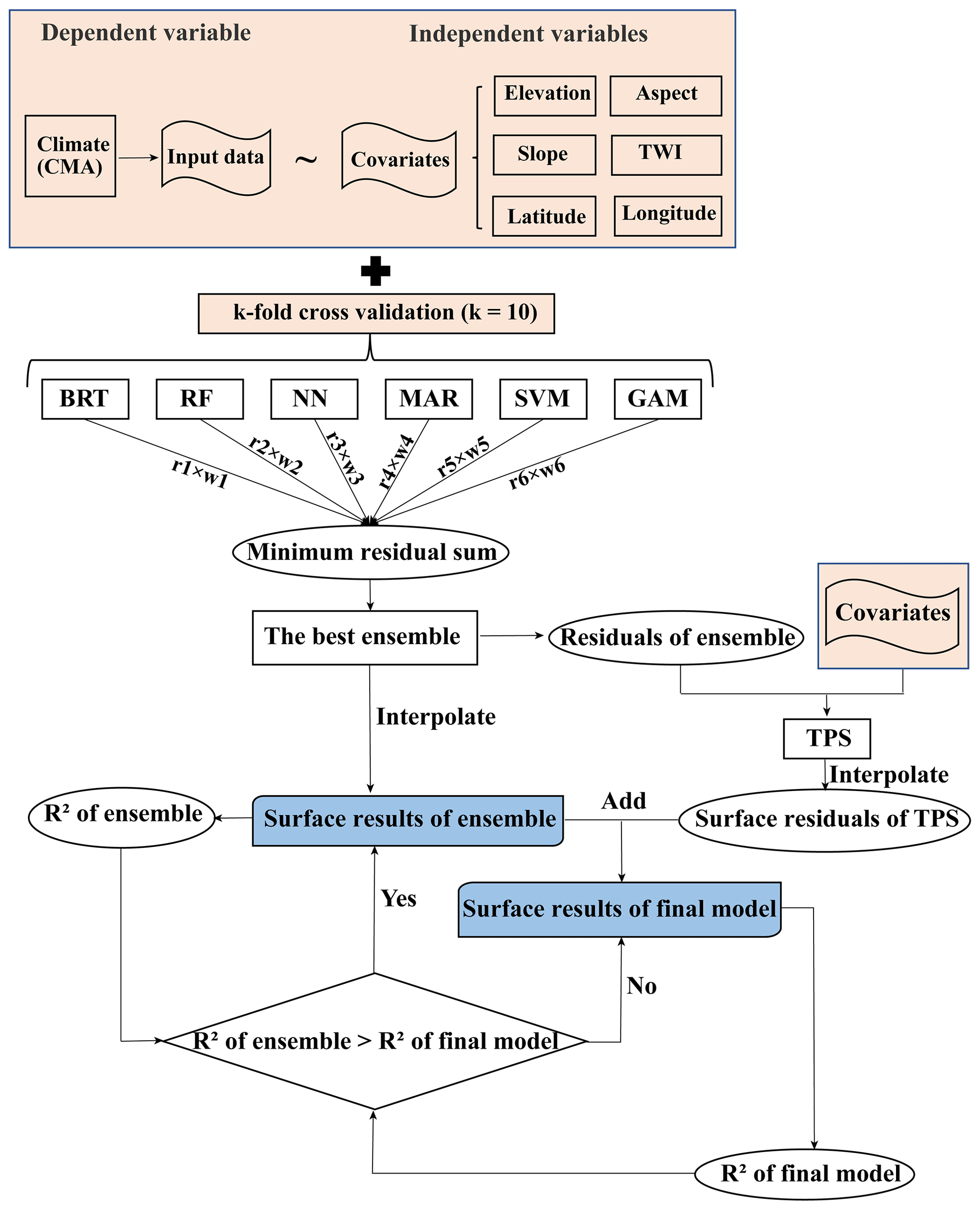
Figure 2The process of spatial interpolation. r1 to r6 are the residual errors from the algorithms, respectively. w1 to w6 are the weights of the algorithms, respectively. BRT, RF, NN, MAR, SVR, GAM, and TPS refer to boosted regression trees, random forests, neural network, multivariate adaptive regression splines, support vector machines, generalized additive model, and thin-plate-smoothing splines, respectively. R2 is the coefficient of determination between the estimated and observed values. TWI is the topographic wetness index.
3.2 The interpolation scheme
As shown in Fig. 2, different combinations of six algorithms – boosted regression trees (BRT), random forests (RF), neural network (NN), multivariate adaptive regression splines (MAR), support vector machines (SVM), and the generalized additive model (GAM) – were used to predict the input data. Firstly, through k-fold cross-validation (k=10), the input data were randomly divided into 10 sub-training datasets and sub-testing datasets. Each algorithm ran in a loop through all the sub-training sets and calculated the residuals from the sub-testing sets. The residuals obtained in each loop were retained. The residual of each algorithm was assigned a weight of 0–1 and the residuals of all the algorithms were summed, and the ensemble of models with the lowest residual sum was chosen. After determining the best ensemble of models, the surface results were interpolated using the best ensemble of models, input data, and covariates. Thin-plate-smoothing splines (TPS) were used to correct the residual error from the ensemble of models. Therefore, residuals of the ensemble were calculated from the input data and these values were interpolated using TPS. Surface results from the ensemble were added to the residuals from the thin-plate-smoothing splines to get the surface results for the final model. The R2 of the surface result for the ensemble was compared to that of the final model, and the surface result with the higher R2 was retained.
3.3 The interpolation methods
We now introduce the individual algorithms (methods) and the implementations for model training (R packages and functions). After model training, the function “predict” in the R package “raster” was used to implement spatial interpolation for the BRT, RF, NN, MAR, SVM, and GAM models, and the function “interpolate” in the R package “raster” was used to perform spatial interpolation with TPS. More details on R packages and functions can be found on the the web (https://www.rdocumentation.org/, last access: 15 September 2022).
3.3.1 The BRT model
A powerful tool for exploratory regression analysis, BRT is a combination of two techniques: decision trees and the boosting method (Elith et al., 2008). BRT can automatically detect the best fit and is robust to missing values and outliers; therefore, BRT is now widely used in remote sensing and in species distribution and meteorological interpolation (Pouteau et al., 2011; Appelhans et al., 2015; Froeschke and Froeschke, 2011). There are two important parameters in BRT: (1) the tree complexity (TC), which controls the number of splits in each tree; (2) the learning rate (LR), which determines the contribution of each tree to the growth model (the smaller the value of LR, the larger the number of trees built). These two parameters together determine the number of trees required for the best prediction in order to find the combination of parameters that leads to the least prediction error. The function “gbm.step” in the R package “dismo” was used for BRT implementation. The tree complexity was set at 5 and the learning rate was set at 0.001. In addition, the “bag.fraction”, which specifies the proportion of data to be selected at each step, was set at 0.5, and other parameters were set at their default values in “gbm.step”.
3.3.2 The RF model
Like BRT, the main technology of RF also includes decision trees; however, the way in which the data used to build the trees are selected is different (the boosting method for BRT, the bagging method for RF). For regression analysis, the bagging method, which takes a random subset of all the data for each new tree that is built, makes the final output based on the average of multiple trees (Breiman, 2001). As it is one of the most accurate algorithms, RF has been used widely for predicting spatiotemporal variables, such as temperature and precipitation (He et al., 2016; Mital et al., 2020; Webb et al., 2016). The function “randomForest” in the R package “randomForest” was used for RF implementation. The importance was set to TRUE and other parameters were set to their default values in “randomForest”.
3.3.3 The NN model
A powerful set of tools for solving problems in pattern recognition, data processing, and nonlinear control (Bishop, 1994), an NN consists of a large number of nodes and connections and includes an input layer, a hidden layer, and an output layer (Lek and Guégan, 1999). Information from each node in the input layer is fed to the hidden layer. Connections between input layer nodes and hidden layer nodes can all be given specific weights according to their importance. The connection between the hidden layer and the output layer is also weighted, so the output is the result of the weighted sum of the hidden nodes. Information is transferred between the hidden layer and the output layer through the transfer function. Since the 1980s, NNs have been used in a number of fields, such as for the prediction of meteorological variables (Snell et al., 2000; Lek and Guégan, 1999; Tang et al., 2020). The function “nnet” in the R package “nnet” was used for NN implementation. The number of units in the hidden layer (size) was set to 10, the transfer function was linear for the output layer (linout was set to TRUE), the maximum number of iterations (maxit) was set to 10 000, and other parameters were set to their default values in “nnet”.
3.3.4 The MAR model
MAR is an extension of the linear model that can build multiple linear regression models within the range of predictive variable values by partitioning data (Friedman, 1991; Friedman and Roosen, 1995). MAR consists of two steps: firstly, it creates a set of so-called basis functions. In this process, the range of predictive variable values is divided into several groups. For each group, a separate linear regression is modeled. Secondly, MAR estimates a least-squares model with its basis function as the independent variable. Overfitting is avoided by iterating to remove the basis functions that contribute least to the model fitting. MAR works well with a large number of predictor variables, it automatically detects interactions between variables, and it is robust to outliers; therefore, studies have done on downscaling or predicting meteorological data using MAR (Panda et al., 2022; D. H. W. Li et al., 2019; Zawadzka et al., 2020). The function “earth” in the R package “earth” was used for MAR implementation. A linear model was used to estimate the standard deviation as a function of the predicted response (varmod.method = “lm”). nfold was set to 10, ncross was set to 30, and other parameters were set to their default values in “earth”.
3.3.5 The SVM model
SVM is another machine learning supervised algorithm, and mainly deals with the ideas of classification and regression (Vapnik, 1999, 1991; Brereton and Lloyd, 2010). SVM is well supported by mathematical theory and can use kernel tricks to efficiently process nonlinear data. With the development of SVM, it has also been widely used in the regression and prediction of meteorological variables (Belaid and Mellit, 2016; Chen et al., 2010; Tripathi et al., 2006). In this study, the function “ksvm” in the R package “kernlab” was used for SVM implementation, and all parameters were set to their default values in “ksvm”.
3.3.6 The GAM model
The GAM is an extension of the generalized linear model (GLM). Like the GLM, the GAM consists of three important components: the probability distribution of the dependent variable, the linear predictor, and the link function; however, in the GAM, the coefficient of the independent variable in the linear regression is replaced by a sum of smooth functions (Hastie and Tibshirani, 1990; Liu, 2008). Because the GAM can deal with nonlinear and nonmonotone relationships between dependent and independent variables, it has been used to predict and interpolate meteorological data (Hjort et al., 2016; Burnett and Anderson, 2019; Aalto et al., 2013). The function “gam” in the R package “mgcv” was used for GAM implementation, and all parameters were set to their default values in “gam”.
3.3.7 The TPS method
A traditional interpolation method, TPS has been widely used to spatially interpolate surface climate data (Gong et al., 2022; Hancock and Hutchinson, 2006; Risk and James, 2022). In this study, it was used to correct the residual error from the ensemble of models. The function “Tps” in the R package “fields” was used for TPS implementation. The matrix of independent variables consisted of the latitude and longitude, the vector of dependent variables consisted of the residual errors in the above algorithms. Other parameters were set to their default values in “Tps” function.
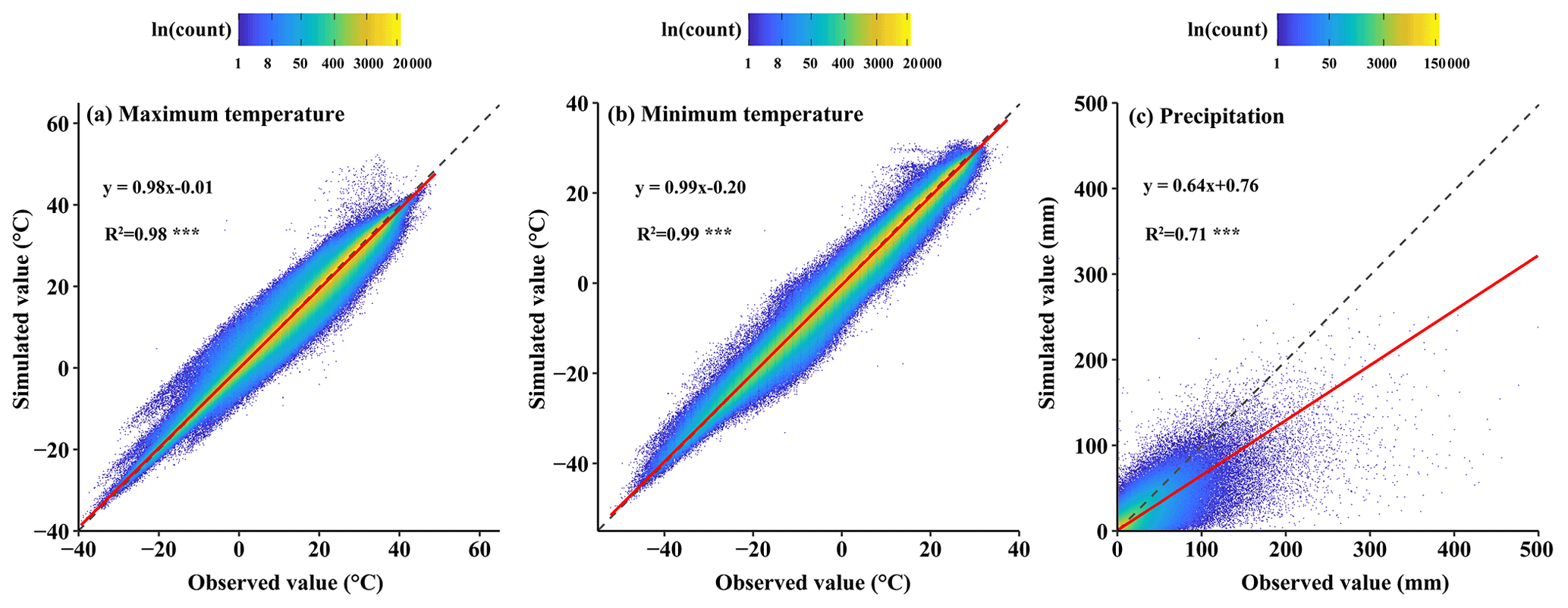
Figure 3Scatter density plots of daily maximum and minimum temperatures and precipitation between estimated and observed values at meteorological stations were used to test the HRLT dataset. The dashed line has a slope of 1 and the red line is a fit between the estimated and observed values. R2 is the coefficient of determination between the estimated and observed values. Asterisks (***) indicate that the significance of the regression equation between the estimated and observed values, p, is <0.001.
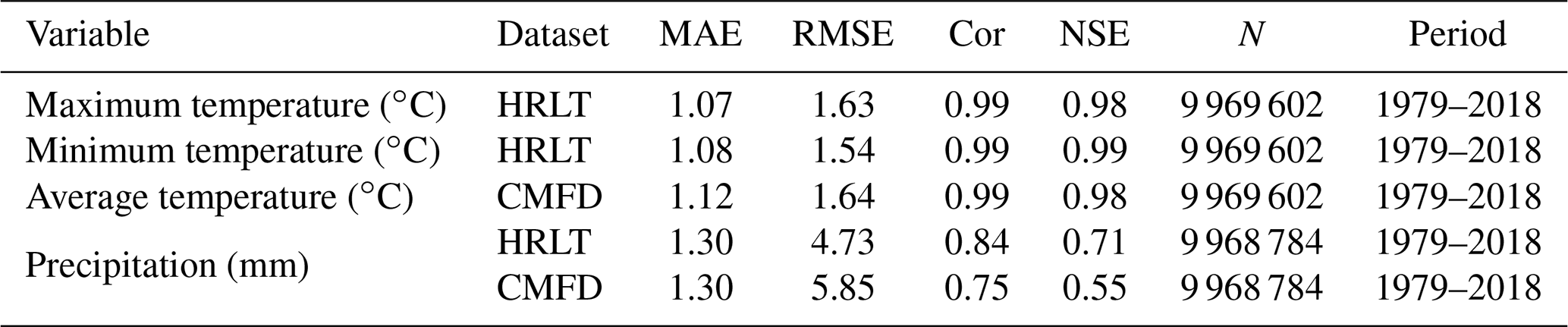
Table 1Summary of the accuracies for the HRLT datasets using data from the meteorological stations.
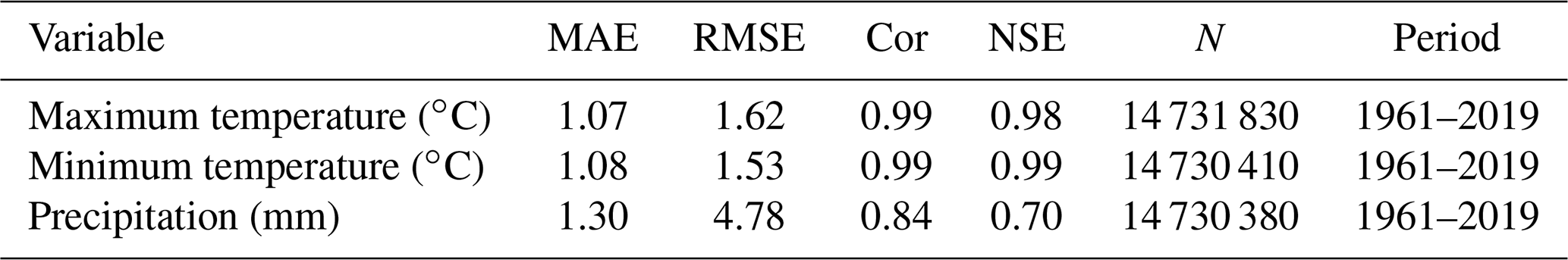
MAE, RMSE, Cor, and NSE are the mean absolute error, root mean square error, Pearson's correlation coefficient, and Nash–Sutcliffe modeling efficiency, respectively. N is the number of observations. Period shows the first and last years covered by the data.
3.4 The interpolation implementation
A complete operation was performed per day per variable, so there were 64 647 operations (21 549 d × 3 variables) from 1 January 1961 to 31 December 2019 for maximum temperature, minimum temperature, and precipitation. A complete operation for a day per variable required a central processing unit core, 18 GB of operating memory, and 2 h of time. In order to shorten the running time, we carried out parallel computing on a supercomputer platform. Spatial interpolation work was executed by R version 4.0.2 (R Core Team, 2018), and the R package “machisplin” (Brown, 2019) was referenced to achieve it.
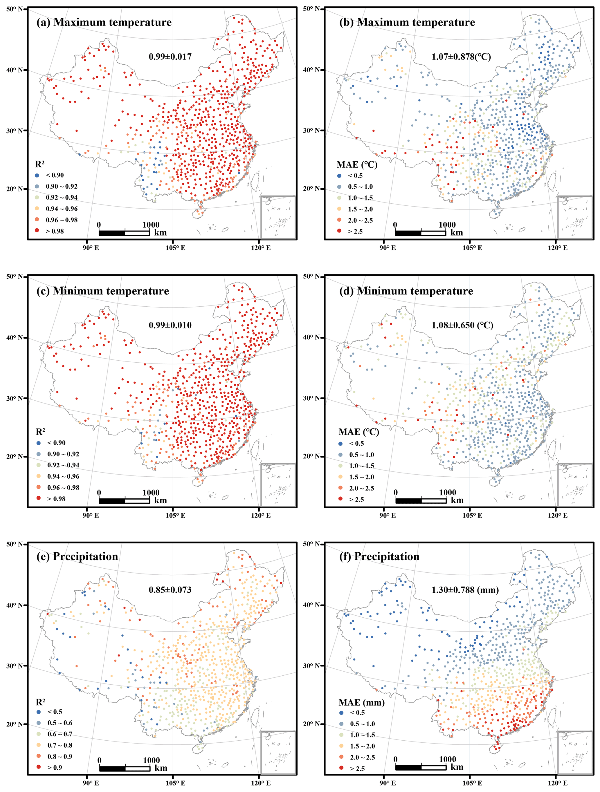
Figure 4Spatial distributions of R2 and MAE for daily maximum temperature, minimum temperature, and precipitation between 1961 and 2019. The value before the ± is the R2 or MAE mean value and the value after the ± is the R2 or MAE standard deviation for all meteorological stations.
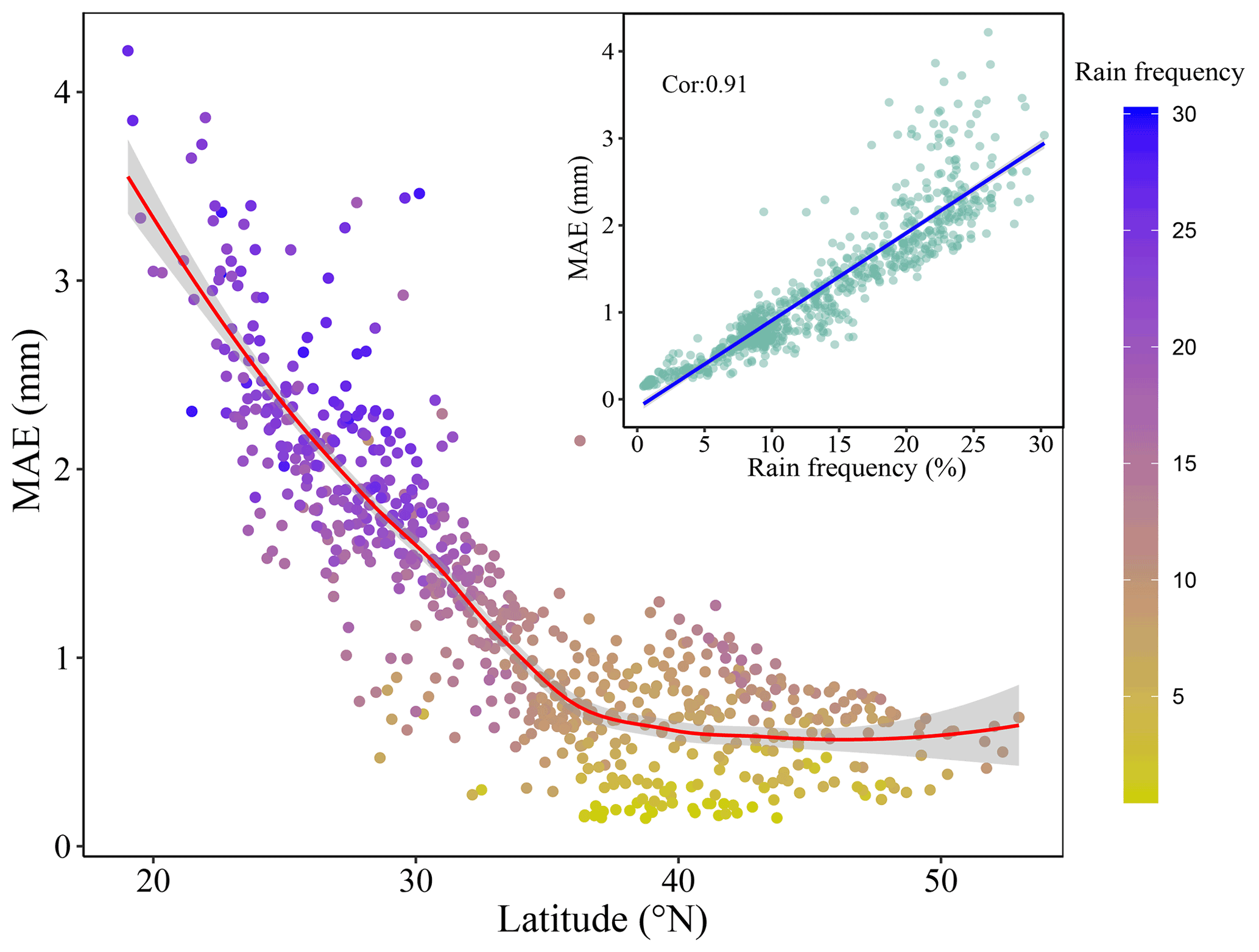
Figure 5The relationship between latitude and MAE of daily precipitation. The inset shows the relationship between rainfall frequency above light rainfall and MAE of daily precipitation. MAE is the mean absolute error. Cor is Pearson's correlation coefficient. Rain frequency is the rainfall frequency above light rainfall, which is defined as the daily rainfall from 0 to 4 mm (Alpert et al., 2002).
3.5 Evaluation metrics
The mean absolute error (MAE), root mean square error (RMSE), Pearson's correlation coefficient (Cor), coefficient of determination after adjustment (R2), and Nash–Sutcliffe modeling efficiency (NSE) were used to evaluate the interpolation results. Pearson's correlation coefficient was used to evaluate the correlation between the simulated and observed values, and the other metrics are defined separately as follows:
where Si and Oi are the model-predicted and the experimentally observed values, respectively; is the mean of the observed values; n is the number of observations; and k is the value of the independent variable. High Cor, R2, and NSE values between the predicted and observed values.
4.1 Validation of temperature and precipitation
The spatial interpolation results, including daily maximum temperature, minimum temperature, and precipitation, were validated using meteorological station data. The results of the validation showed that the daily maximum and minimum temperatures were highly accurate (Fig. 3 and Table 1). The fitting slopes between the simulated and observed values were both close to 1 and the coefficients of determination after adjustment were 0.98 and 0.99, respectively, for daily maximum and minimum temperature (Fig. 3a and b). As shown in Table 1, the MAE was 1.07 and 1.08 ∘C and the RMSE was 1.62 and 1.53 ∘C for daily maximum and minimum temperatures, respectively. In addition, the Cor and NSE values were close to 1 for both the daily maximum and the daily minimum temperatures. Daily precipitation was less accurate than temperature, with an R2 of 0.71 (Fig. 3c), which was mainly caused by underestimating the high daily precipitation. However, most of the points were concentrated in the low daily precipitation section. Furthermore, the MAE and RMSE for daily precipitation were 1.30 and 4.78 mm, respectively; the Cor between the simulated and observed daily precipitation was 0.84, and the NSE was 0.70 (Table 1).
The interpolation accuracy shows spatial differences (Fig. 4). The R2 values of the daily maximum and minimum temperatures in Southwest China were less than 0.94 and lower than those for other regions (Fig. 4a and c). The mean absolute errors for the daily maximum and minimum temperature ranges at most meteorological stations were less than 1 ∘C. However, there were some meteorological stations with mean absolute errors of more than 2 ∘C, and these were evenly distributed across China (Fig. 4b and d). The R2 value for daily precipitation at most meteorological stations was greater than 0.7 and the MAE decreased from south to north across China (Fig. 4e and f). For precipitation, the R2 map (Fig. 4e) shows a west–east gradient in the scores, which is different from the north–south gradient present in the MAE map (Fig. 4f). There are fewer meteorological observation stations in the western region than in the eastern region, which may lead to the subtle east–west gradient in R2 for daily precipitation. The obvious north–south gradient for MAE of daily precipitation could be caused by the rainfall frequency (Figs. 4f, 5); the MAE of monthly precipitation in China from another study showed a similar pattern (Peng et al., 2019). Rainfall frequency above light rainfall, which is defined as daily rainfall ranging from 0 to 4 mm (Alpert et al., 2002), is strongly correlated with the MAE of daily precipitation (illustration in Fig. 5), so that the MAE of daily precipitation in the southern region with a higher rainfall frequency is larger than that in the northern region with a lower rainfall frequency.
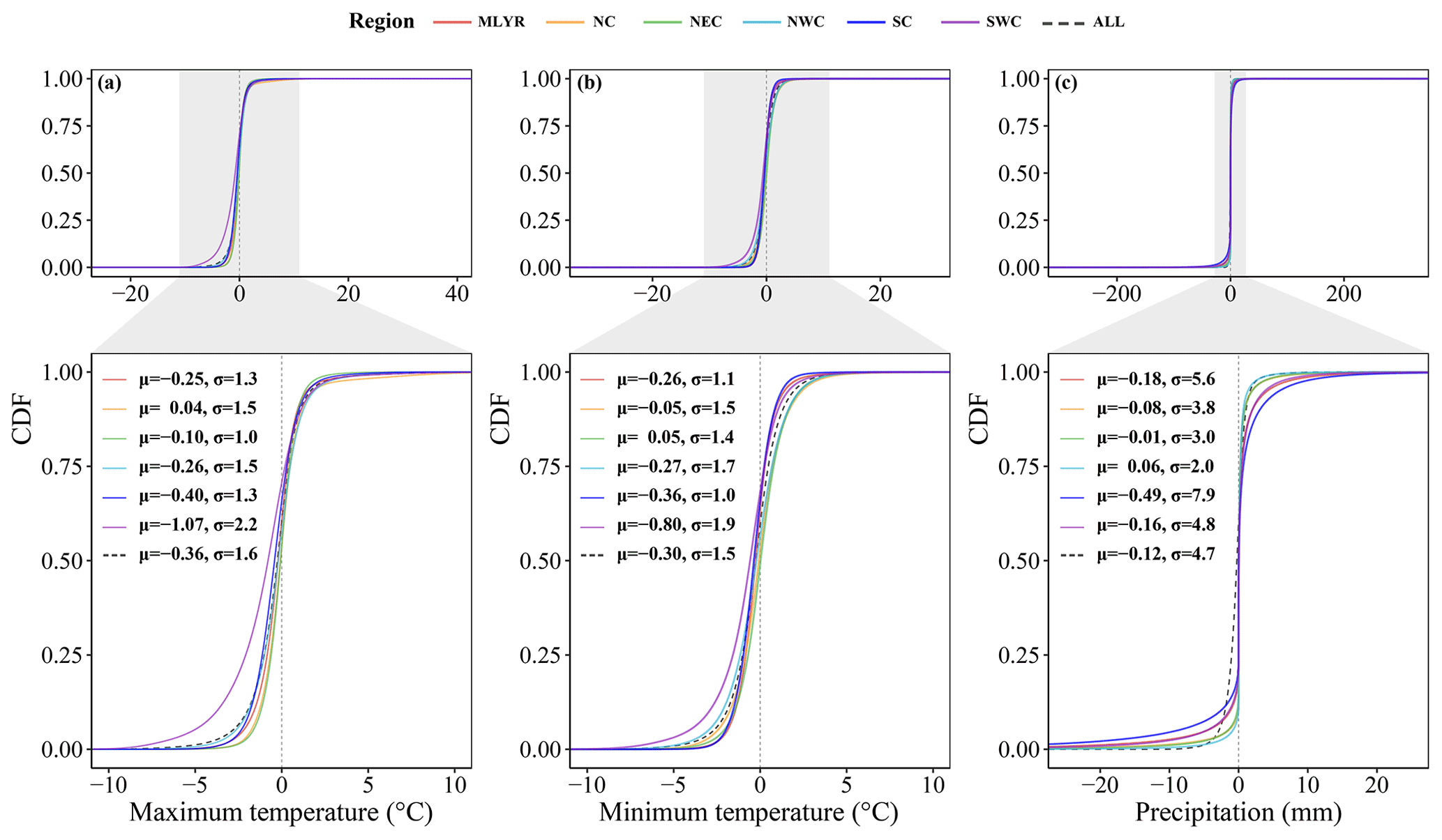
Figure 6Cumulative distribution functions (CDFs) of the difference between the estimated and observed values for three variables at all meteorological stations from 1961 to 2020. μ is the mean and σ is the standard deviation. MLYR, NC, NEC, NWC, SC, and SWC are the middle and lower reaches of the Yangtze River, North China, Northeast China, Northwest China, South China, and Southwest China, respectively.
The meteorological stations were divided into the middle and lower reaches of the Yangtze River (MLYR), North China (NC), Northeast China (NEC), Northwest China (NWC), South China (SC), and Southwest China (SWC) (Fig. 1) according to their diverse geographic and climatic conditions and administrative areas (Qin et al., 2022). The trend in the cumulative distribution function curve of the difference between the simulated and observed values was always similar for daily maximum temperature, minimum temperature, and precipitation in the six regions, as well as for the whole of China. The daily maximum and minimum temperatures were all underestimated in the MLYR, NEC, NWC, SC, and SWC (Fig. 6a). The daily minimum temperatures were all underestimated in the MLYR, NC, NWC, SC, and SWC (Fig. 6b). For both daily maximum and minimum temperatures, the lowest average difference between the simulated and observed values occurred in NC and NEC, while the greatest difference occurred in SWC (Fig. 6a and b). Except in the NWC region, the average difference between simulated and observed values for daily precipitation was less than 0 mm in the regions (Fig. 6c). The largest average difference between simulated and observed values for daily precipitation occurred in the SC region, with a value of 0.49 mm (Fig. 6c). Across the whole of China, the average difference between simulated and observed values for daily maximum temperature, minimum temperature, and precipitation was 0.36 ∘C, 0.30 ∘C, and 0.12 mm, respectively.

Figure 7Spatial distributions of annual average values for the daily maximum and minimum temperatures and annual precipitation in 1965, 1980, 1990, and 2010. The regions within the ellipses are where the change is most visible.
4.2 Temporal and spatial distributions of temperature and precipitation
The results showed that detailed spatial changes in temperature and precipitation over time could be obtained (Fig. 7). For example, the increases in the annual average values of both maximum temperature and minimum temperature were obvious over the Tibetan Plateau from 1965 to 2010 (Fig. 7a–h, the d1 and h1 subregions). In addition, compared with other years, the annual average daily minimum temperature clearly increased in some areas of NWC (Fig. 7e–h, the h2 and h3 subregions) and MLYR (Fig. 7e–h, the h4 subregion) in 2010. The most significant annual precipitation changes occurred in NEC (Fig. 7i–l, the l1 subregion) between 1965 and 2010.

Figure 8Density distributions of annual average values for the daily maximum and minimum temperatures and annual precipitation across the different regions in 1965, 1980, 1990, and 2010. The values shown in the plots are mean values.
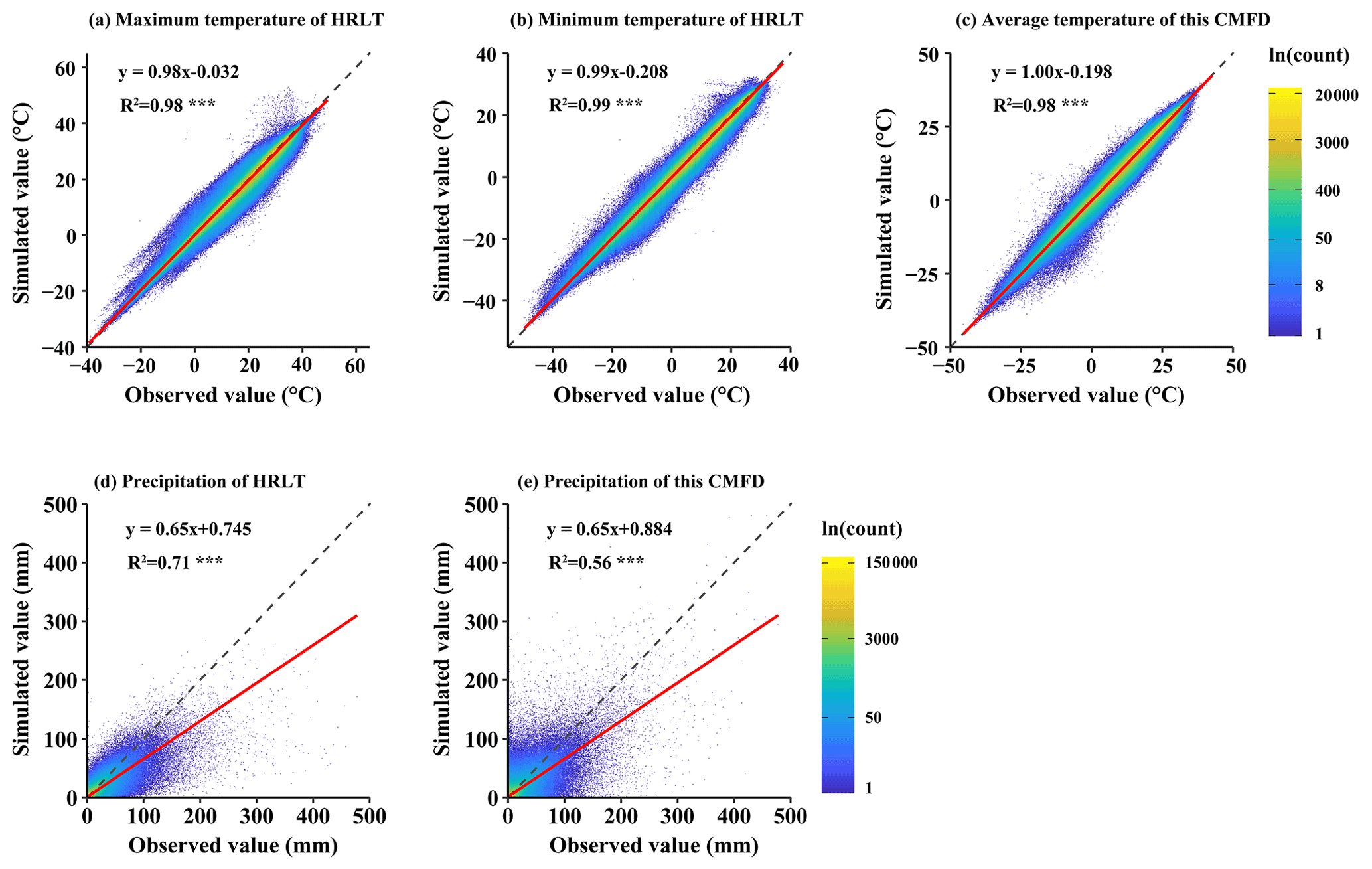
Figure 9Scatter density plots of the estimated versus the observed values of daily temperature and precipitation at all meteorological stations (both training sets and testing sets) for the HRLT dataset and the CMFD dataset between 1979 and 2018. The dashed line has a slope of 1 and the red line is a fit between the estimated and observed values. R2 is the coefficient of determination between the estimated and observed values. Asterisks (***) indicate that the significance of the regression equation between the estimated and observed values, p, is <0.001.

Figure 10Scatter density plots of the estimated versus the observed values of daily temperature and precipitation at all meteorological stations (both training sets and testing sets) for our HRLT dataset and the CLDAS dataset between 2017 and 2019. The dashed line has a slope of 1 and the red line is a fit between the estimated and observed values. R2 is the coefficient of determination between the estimated and observed values. Asterisks (***) indicate that the significance of the regression equation between the estimated and observed values, p, is <0.001.
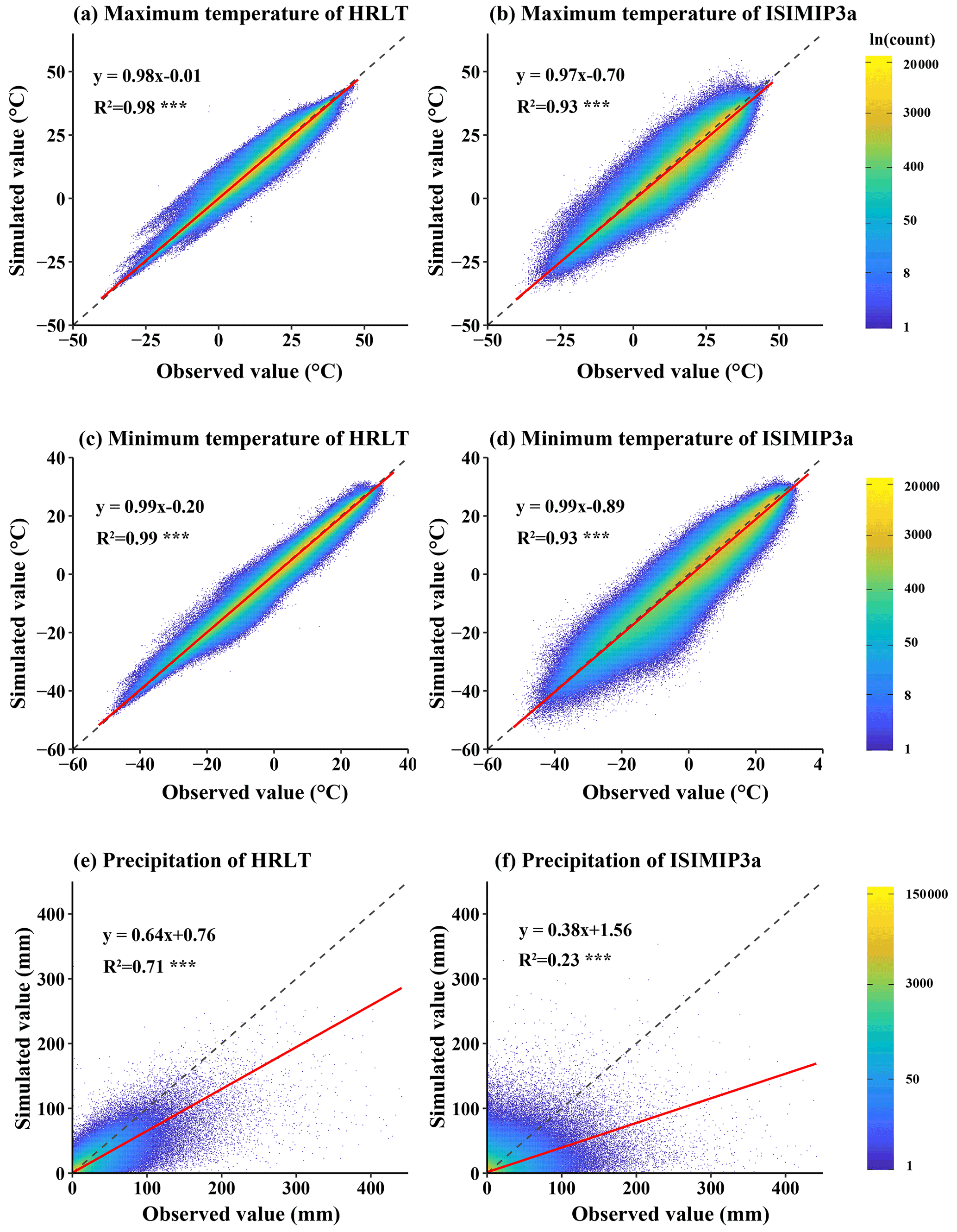
Figure 11Scatter density plots of the estimated versus the observed values of daily temperature and precipitation at all meteorological stations (both training sets and testing sets) for our HRLT dataset and the ISIMIP3a dataset between 1961 and 2016. The dashed line has a slope of 1 and the red line is a fit between the estimated and observed values. R2 is the coefficient of determination between the estimated and observed values. Asterisks (***) indicate that the significance of the regression equation between the estimated and observed values, p, is <0.001.
The distributions of annual average daily maximum and minimum temperatures and annual precipitation across the six regions of China in 1965, 1980, 1995, and 2010 were analyzed (Fig. 8). Compared with other years, the areas with smaller values for annual average daily maximum temperature (less than 0) and annual average daily minimum temperature (less than −10) in SWC and NWC decreased in 2010 (Fig. 8a1, a2, b1, b2). These areas are mainly distributed on the Qinghai–Tibet Plateau, which has seen a large increase in temperature over the past few decades. The density distribution peaks for the annual average daily maximum and minimum temperatures in NEC moved to the right from 1965 to 1995 but moved to the left in 2010 (Fig. 8a3 and b3). The mean annual average daily minimum temperature in 2010 was higher in the MLYR, NC, and SC than in the other 3 years (Fig. 8b4–b6). There was an increase in mean annual precipitation in the northern part of China over the period 1965–2010 (Fig. 8c2–c4). It increased from 335 to 415 mm across NWC (Fig. 8c2), from 487 to 593 mm across NEC (Fig. 8c3), and from 531 to 654 mm across NC (Fig. 8c4). In the MLYR, there were more areas with an annual precipitation of less than 1000 mm, and areas with an annual precipitation of more than 2000 mm increased in 1995 and 2010 compared with 1965 and 1980 (Fig. 8c5). Similarly, compared with other years, there were more areas with an annual precipitation of less than 1000 mm and more than 2000 mm in SC in 2010 (Fig. 8c6).
Table 2Comparison of accuracies for the HRLT and CMFD datasets using data from the meteorological stations.
MAE, RMSE, Cor, and NSE are the mean absolute error, root mean square error, Pearson's correlation coefficient, and Nash–Sutcliffe modeling efficiency, respectively. N is the number of observations. Period shows the first and last years covered by the data.
Table 3Comparison of accuracies for the HRLT and the CLDAS datasets using data from the meteorological stations.
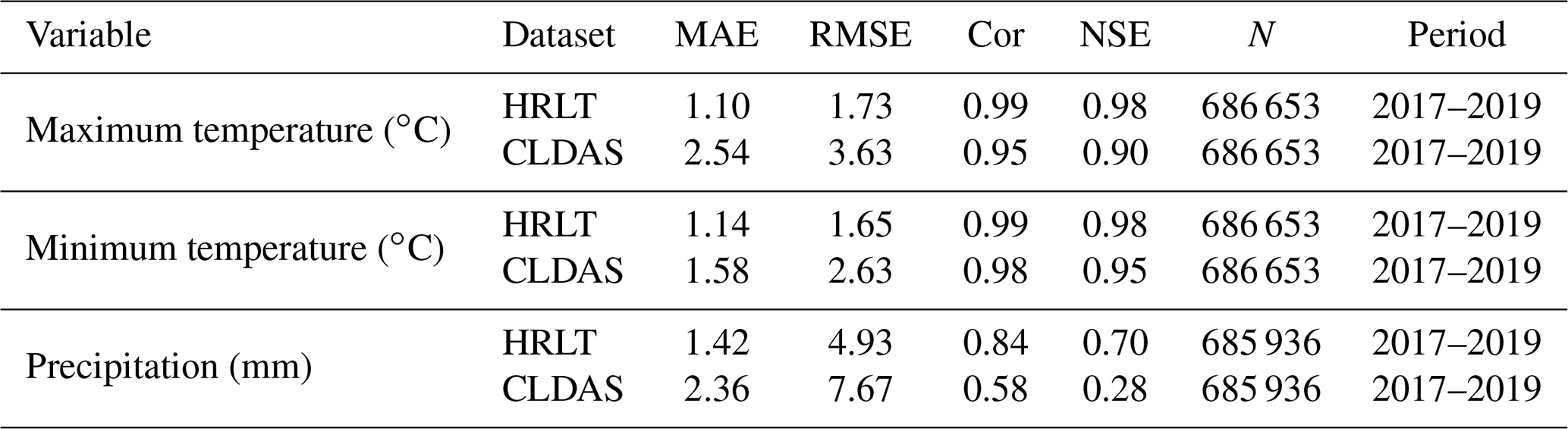
MAE, RMSE, Cor, and NSE are the mean absolute error, root mean square error, Pearson's correlation coefficient, and Nash–Sutcliffe modeling efficiency, respectively. N is the number of observations. Period shows the first and last years covered by the data.
Table 4Comparison of accuracies for the HRLT and the ISIMP3a datasets using data from the meteorological stations.
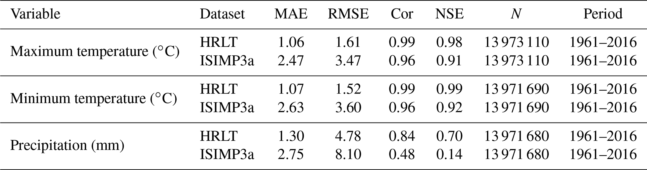
MAE, RMSE, Cor, and NSE are the mean absolute error, root mean square error, Pearson's correlation coefficient, and Nash–Sutcliffe modeling efficiency, respectively. N is the number of observations. Period shows the first and last years covered by the data.
4.3 Accuracy comparison with other products
The performances of the CMFD, CLDAS, and ISIMIP3a generated daily temperatures and precipitations were evaluated against observations from all the meteorological stations, and their performances were compared with that of our dataset (Figs. 9–11; Tables 2–4). The fitting slopes between the simulated and observed daily temperature values were always close to 1 for all datasets (Figs. 9a–c, 10a–d, 11a–d). The R2 for the CMFD daily average temperature was slightly smaller than that for daily minimum temperature in our dataset (Fig. 9b and c), but was equal to that of our dataset for daily maximum temperature (Fig. 9a and c). The Cor and NSE for the CMFD daily average temperature were also similar to those for our estimated daily maximum and minimum temperatures (Table 2). By contrast, the MAE and RMSE for the CMFD daily average temperature were 1.12 and 1.64 ∘C, respectively, which were greater than those for our estimated daily maximum and minimum temperatures (Table 2). The MAEs of daily maximum and minimum temperature for our dataset were 1.07 and 1.08 ∘C, respectively, and the RMSEs of daily maximum and minimum temperature for our dataset were 1.63 and 1.54 ∘C, respectively, between 1979 and 2018 (Table 2). The R2, Cor, NSE, MAE, and RMSE for the CLDAS daily maximum temperature were 0.91, 0.95, 0.90, 2.54, and 3.63 ∘C, respectively. Accuracy was clearly improved for our daily maximum temperature, and the corresponding metrics were 0.98, 0.99, 0.98, 1.10, and 1.73 ∘C (Fig. 10a and b; Table 3). The MAE and RMSE for the CLDAS daily minimum temperature were clearly higher than our estimates for daily minimum temperature, and the R2, Cor, and NSE for daily minimum temperature in our dataset were higher than those for the CLDAS daily minimum temperature (Fig. 10c and d; Table 3), thus indicating that the accuracy of our daily minimum temperature estimates was superior to that of the CLDAS daily minimum temperature product. Compared with those of the ISIMIP3a, the R2, Cor, and NSE of the daily maximum and minimum temperatures in our dataset were always higher and the MAE and RMSE of those temperatures were always smaller (Fig. 11a–d; Table 4).
The R2 value for our estimated daily precipitation was clearly improved compared to the other three datasets, especially the ISIMIP3a and CLDAS datasets (Figs. 9d and e, 10e and f, 11e and f). The Cor and NSE for the CMFD daily precipitation were clearly smaller than those for our dataset, and the RMSE for CMFD daily precipitation was greater than that for our dataset (Table 2). During 2017–2019, the Cor, NSE, MAE, and RMSE for our estimated daily precipitation were 0.84, 0.70, 1.42, and 4.93 mm, respectively, and the corresponding values for the CLDAS daily precipitation changed to 0.58, 0.28, 2.36, and 7.67 mm, respectively (Table 3). During 1961–2016, the Cor, NSE, MAE, and RMSE for our estimated daily precipitation were 0.84, 0.70, 1.30, and 4.78 mm, respectively, and the corresponding values for the ISIMIP3a daily precipitation changed to 0.48, 0.14, 2.75, and 8.10 mm, respectively (Table 4). Thus, the daily precipitation accuracy of our dataset was generally higher than those of CMFD, CLDAS, and ISIMIP3a.
The HRLT dataset includes daily maximum temperature, minimum temperature, and precipitation at 1 km spatial resolution across China from January 1961 to December 2019. The datasets are publicly available in NetCDF format at https://doi.org/10.1594/PANGAEA.941329 (Qin and Zhang, 2022).
The result of this study is a long-term (1961–2019), high-resolution (1 km) daily gridded maximum temperature, minimum temperature, and precipitation dataset across China (HRLT). The HRLT dataset shows a high correlation overall with the observations from meteorological stations for daily maximum and minimum temperatures (R2 was 0.98 and 0.99, respectively; Cor was 0.99 for both; NSE was 0.98 and 0.99, respectively), and the errors were small (MAE was 1.07 and 1.08 ∘C, respectively; RMSE was 1.62 and 1.53 ∘C, respectively). Although the HRLT dataset showed that the daily precipitation accuracy was lower than the daily temperature accuracy (R2, Cor, NSE, MAE, and RMSE were 0.71, 0.84, 0.70, 1.30, and 4.78 mm, respectively), the daily precipitation data in the HRLT dataset were more accurate and had a finer spatial resolution compared to three other existing datasets (CMFD, CLDAS, and ISIMIP3a). Furthermore, the accuracies for daily maximum and minimum temperatures and precipitation were lower in the southwestern part of China, probably because of the complex topography in that area compared to other areas. Calculation and interpolation by subregion may solve this problem in future studies. The use of satellite data as an input covariate in future studies will further improve the accuracy of the HRLT dataset, especially for precipitation. The HRLT dataset will help identify future extreme climatic events and can also be used to improve process-based models for prediction, adaptation, and mitigation strategies.
RQ and FZ calculated the dataset, analyzed the results, and wrote the manuscript; all other authors reviewed and revised the manuscript.
The contact author has declared that none of the authors has any competing interests.
Publisher's note: Copernicus Publications remains neutral with regard to jurisdictional claims in published maps and institutional affiliations.
We thank the Supercomputing Center of Lanzhou University for providing the computing requirements for this study. We are also grateful to the China Meteorological Data Service Centre, National Tibetan Plateau Third Pole Environment Data Center, Potsdam Institute for Climate Impact Research, and the International Institute for Applied Systems Analysis for contributing datasets to the study. We also thank Marianne Rehage from PANGAEA for processing and publishing the dataset.
This research has been supported by the Second Tibetan Plateau Scientific Expedition and Research (grant no. 2019QZKK0305), the National Natural Science Foundation of China (grant no. 32071550), the Fundamental Research Funds for the Central Universities (grant no. lzujbky-2022-41), the “111” Programme (BP0719040), and the Science and Technology Programme of Gansu Province (2022CXZX-152).
This paper was edited by Christof Lorenz and reviewed by two anonymous referees.
Aalto, J., Pirinen, P., Heikkinen, J., and Venäläinen, A.: Spatial interpolation of monthly climate data for Finland: comparing the performance of kriging and generalized additive models, Theor. Appl. Climatol., 112, 99–111, https://doi.org/10.1007/s00704-012-0716-9, 2013.
Alpert, P., Ben-Gai, T., Baharad, A., Benjamini, Y., Yekutieli, D., Colacino, M., Diodato, L., Ramis, C., Homar, V., Romero, R., Michaelides, S., and Manes, A.: The paradoxical increase of Mediterranean extreme daily rainfall in spite of decrease in total values, Geophys. Res. Lett., 29, 31–1, https://doi.org/10.1029/2001GL013554, 2002.
Appelhans, T., Mwangomo, E., Hardy, D. R., Hemp, A., and Nauss, T.: Evaluating machine learning approaches for the interpolation of monthly air temperature at Mt. Kilimanjaro, Tanzania, Spatial Stat., 14, 91–113, https://doi.org/10.1016/j.spasta.2015.05.008, 2015.
Belaid, S. and Mellit, A.: Prediction of daily and mean monthly global solar radiation using support vector machine in an arid climate, Energ. Convers. Manage., 118, 105–118, https://doi.org/10.1016/j.enconman.2016.03.082, 2016.
Bishop, C. M.: Neural networks and their applications, Rev. Sci. Instr., 65, 1803–1832, https://doi.org/10.1063/1.1144830, 1994.
Breiman, L.: Random forests, Mach. Learn., 45, 5–32, 2001.
Brereton, R. G. and Lloyd, G. R.: Support Vector Machines for classification and regression, Analyst, 135, 230–267, https://doi.org/10.1039/B918972F, 2010.
Brinckmann, S., Krähenmann, S., and Bissolli, P.: High-resolution daily gridded data sets of air temperature and wind speed for Europe, Earth Syst. Sci. Data, 8, 491–516, https://doi.org/10.5194/essd-8-491-2016, 2016.
Brown, J. L.: Interpolation of noisy multi-variate data using machine learning ensembling, GitHub [code], https://github.com/jasonleebrown/machisplin (last access: 30 Oct 2022), 2019.
Burnett, J. D. and Anderson, P. D.: Using generalized additive models for interpolating microclimate in dry-site ponderosa pine forests, Agric. Forest Meteorol., 279, 107668, https://doi.org/10.1016/j.agrformet.2019.107668, 2019.
Chen, S.-T., Yu, P.-S., and Tang, Y.-H.: Statistical downscaling of daily precipitation using support vector machines and multivariate analysis, J. Hydrol., 385, 13–22, https://doi.org/10.1016/j.jhydrol.2010.01.021, 2010.
Chen, Y., Liang, S., Ma, H., Li, B., He, T., and Wang, Q.: An all-sky 1 km daily land surface air temperature product over mainland China for 2003–2019 from MODIS and ancillary data, Earth Syst. Sci. Data, 13, 4241–4261, https://doi.org/10.5194/essd-13-4241-2021, 2021.
Elith, J., Leathwick, J. R., and Hastie, T.: A working guide to boosted regression trees, J. Anim. Ecol., 77, 802–813, https://doi.org/10.1111/j.1365-2656.2008.01390.x, 2008.
Friedman, J. H.: Multivariate adaptive regression splines, Ann. Stat., 19, 1–67, https://doi.org/10.1214/aos/1176347963, 1991.
Friedman, J. H. and Roosen, C. B.: An introduction to multivariate adaptive regression splines, Stat. Meth. Med. Res., 3, 192–217, https://doi.org/10.1177/096228029500400303, 1995.
Froeschke, J. T. and Froeschke, B. F.: Spatio-temporal predictive model based on environmental factors for juvenile spotted seatrout in Texas estuaries using boosted regression trees, Fish. Res., 111, 131–138, https://doi.org/10.1016/j.fishres.2011.07.008, 2011.
Gong, H., Liu, H., Xiang, X., Jiao, F., Cao, L., and Xu, X.: 1 km Monthly Precipitation and Temperatures Dataset for China from 1952 to 2019 based on a Brand-New and High-Quality Baseline Climatology Surface, Earth Syst. Sci. Data Discuss. [preprint], https://doi.org/10.5194/essd-2022-45, 2022.
Hancock, P. A. and Hutchinson, M. F.: Spatial interpolation of large climate data sets using bivariate thin plate smoothing splines, Environ. Model. Softw., 21, 1684–1694, https://doi.org/10.1016/j.envsoft.2005.08.005, 2006.
Hartl, L., Stuefer, M., Saito, T., and Okura, Y.: History and Data Records of the Automatic Weather Station on Denali Pass (5715 m), 1990–2007, J. Appl. Meteorol. Climatol., 59, 2113–2127, https://doi.org/10.1175/jamc-d-20-0082.1, 2020.
Hastie, T. J. and Tibshirani, R. J.: Generalized Additive Models, in: 1st Edn., Routledge, https://doi.org/10.1201/9780203753781, 1990.
He, J., Yang, K., Tang, W., Lu, H., Qin, J., Chen, Y., and Li, X.: The first high-resolution meteorological forcing dataset for land process studies over China, Sci. Data, 7, 25, https://doi.org/10.1038/s41597-020-0369-y, 2020.
He, Q., Wang, M., Liu, K., Li, K., and Jiang, Z.: GPRChinaTemp1km: a high-resolution monthly air temperature data set for China (1951–2020) based on machine learning, Earth Syst. Sci. Data, 14, 3273–3292, https://doi.org/10.5194/essd-14-3273-2022, 2022.
He, X., Chaney, N. W., Schleiss, M., and Sheffield, J.: Spatial downscaling of precipitation using adaptable random forests, Water Resour. Res., 52, 8217–8237, https://doi.org/10.1002/2016WR019034, 2016.
Herrera, S., Cardoso, R. M., Soares, P. M., Espírito-Santo, F., Viterbo, P., and Gutiérrez, J. M.: Iberia01: a new gridded dataset of daily precipitation and temperatures over Iberia, Earth Syst. Sci. Data, 11, 1947–1956, https://doi.org/10.5194/essd-11-1947-2019, 2019.
Hjort, J., Suomi, J., and Käyhkö, J.: Extreme urban–rural temperatures in the coastal city of Turku, Finland: Quantification and visualization based on a generalized additive model, Sci. Total Environ., 569, 507–517, https://doi.org/10.1016/j.scitotenv.2016.06.136, 2016.
Iizumi, T., Furuya, J., Shen, Z., Kim, W., Okada, M., Fujimori, S., Hasegawa, T., and Nishimori, M.: Responses of crop yield growth to global temperature and socioeconomic changes, Sci. Rep.-UK, 7, 7800, https://doi.org/10.1038/s41598-017-08214-4, 2017.
Lee, M.-H., Im, E.-S., and Bae, D.-H.: Impact of the spatial variability of daily precipitation on hydrological projections: A comparison of GCM- and RCM-driven cases in the Han River basin, Korea, Hydrol. Process., 33, 2240–2257, https://doi.org/10.1002/hyp.13469, 2019.
Lek, S. and Guégan, J. F.: Artificial neural networks as a tool in ecological modelling, an introduction, Ecol. Model., 120, 65–73, https://doi.org/10.1016/S0304-3800(99)00092-7, 1999.
Lesk, C., Rowhani, P., and Ramankutty, N.: Influence of extreme weather disasters on global crop production, Nature, 529, 84–87, https://doi.org/10.1038/nature16467, 2016.
Li, D. H. W., Chen, W., Li, S., and Lou, S.: Estimation of hourly global solar radiation using Multivariate Adaptive Regression Spline (MARS) – A case study of Hong Kong, Energy, 186, 115857, https://doi.org/10.1016/j.energy.2019.115857, 2019.
Li, T., Zheng, X., Dai, Y., Yang, C., Chen, Z., Zhang, S., Wu, G., Wang, Z., Huang, C., Shen, Y., and Liao, R.: Mapping near-surface air temperature, pressure, relative humidity and wind speed over Mainland China with high spatiotemporal resolution, Adv. Atmos. Sci., 31, 1127–1135, https://doi.org/10.1007/s00376-014-3190-8, 2014.
Li, Y., Guan, K., Schnitkey, G. D., DeLucia, E., and Peng, B.: Excessive rainfall leads to maize yield loss of a comparable magnitude to extreme drought in the United States, Global Change Biol., 25, 2325–2337, https://doi.org/10.1111/gcb.14628, 2019.
Liu, H.: Generalized additive model, Department of Mathematics and Statistics University of Minnesota Duluth, Duluth, MN, USA, 55812, 2008.
Lobell, D. B., Schlenker, W., and Costa-Roberts, J.: Climate Trends and Global Crop Production Since 1980, Science, 333, 616–620, https://doi.org/10.1126/science.1204531, 2011.
Lu, Y., Hu, H., Li, C., and Tian, F.: Increasing compound events of extreme hot and dry days during growing seasons of wheat and maize in China, Sci. Rep.-UK, 8, 16700, https://doi.org/10.1038/s41598-018-34215-y, 2018.
Merino, A., Guerrero-Higueras, A. M., López, L., Gascón, E., Sánchez, J. L., Lorente, J. M., Marcos, J. L., Matía, P., Ortiz de Galisteo, J. P., Nafría, D., Fernández-González, S., Weigand, R., Hermida, L., and García-Ortega, E.: Development of tools for evaluating rainfall estimation models in real- time using the Integrated Meteorological Observation Network in Castilla y León (Spain), EGU General Assembly Conference Abstracts, 10234, https://ui.adsabs.harvard.edu/abs/2014EGUGA..1610234M (last access: 31 October 2022), 2014.
Mital, U., Dwivedi, D., Brown, J. B., Faybishenko, B., Painter, S. L., and Steefel, C. I.: Sequential Imputation of Missing Spatio-Temporal Precipitation Data Using Random Forests, Front. Water, 2, 2624–9375, https://doi.org/10.3389/frwa.2020.00020, 2020.
Myhre, G., Alterskjær, K., Stjern, C. W., Hodnebrog, Ø., Marelle, L., Samset, B. H., Sillmann, J., Schaller, N., Fischer, E., Schulz, M., and Stohl, A.: Frequency of extreme precipitation increases extensively with event rareness under global warming, Sci. Rep.-UK, 9, 16063, https://doi.org/10.1038/s41598-019-52277-4, 2019.
Panda, K. C., Singh, R. M., Thakural, L. N., and Sahoo, D. P.: Representative grid location-multivariate adaptive regression spline (RGL-MARS) algorithm for downscaling dry and wet season rainfall, J. Hydrol., 605, 127381, https://doi.org/10.1016/j.jhydrol.2021.127381, 2022.
Peng, S., Ding, Y., Liu, W., and Li, Z.: 1 km monthly temperature and precipitation dataset for China from 1901 to 2017, Earth Syst. Sci. Data, 11, 1931–1946, https://doi.org/10.5194/essd-11-1931-2019, 2019.
Pouteau, R., Rambal, S., Ratte, J.-P., Gogé, F., Joffre, R., and Winkel, T.: Downscaling MODIS-derived maps using GIS and boosted regression trees: The case of frost occurrence over the arid Andean highlands of Bolivia, Remote Sens. Environ., 115, 117–129, https://doi.org/10.1016/j.rse.2010.08.011, 2011.
Qin, R. and Zhang, F.: HRLT: A high-resolution (1 day, 1 km) and long-term (1961–2019) gridded dataset for temperature and precipitation across China, PANGAEA [data set], https://doi.org/10.1594/PANGAEA.941329, 2022.
Qin, R., Zhang, F., Yu, C., Zhang, Q., Qi, J., and Li, F.-M.: Contributions made by rain-fed potato with mulching to food security in China, Eur. J. Agron., 133, 126435, https://doi.org/10.1016/j.eja.2021.126435, 2022.
Rao, B. B., Chowdary, P. S., Sandeep, V. M., Pramod, V. P., and Rao, V. U. M.: Spatial analysis of the sensitivity of wheat yields to temperature in India, Agr. Forest Meteorol., 200, 192–202, https://doi.org/10.1016/j.agrformet.2014.09.023, 2015.
R Core Team: R: A Language and Environment for Statistical Computing (3.5), R Core Team, https://www.R-project.org/ (last access: 30 October 2020), 2018.
Risk, C. and James, P. M. A.: Optimal Cross-Validation Strategies for Selection of Spatial Interpolation Models for the Canadian Forest Fire Weather Index System, Earth Space Sci., 9, e2021EA002019, https://doi.org/10.1029/2021EA002019, 2022.
Sadeghi, M., Nguyen, P., Naeini, M. R., Hsu, K., Braithwaite, D., and Sorooshian, S.: PERSIANN-CCS-CDR, a 3-hourly 0.04∘ global precipitation climate data record for heavy precipitation studies, Sci. Data, 8, 157, https://doi.org/10.1038/s41597-021-00940-9, 2021.
Schamm, K., Ziese, M., Becker, A., Finger, P., Meyer-Christoffer, A., Schneider, U., Schröder, M., and Stender, P.: Global gridded precipitation over land: a description of the new GPCC First Guess Daily product, Earth Syst. Sci. Data, 6, 49–60, https://doi.org/10.5194/essd-6-49-2014, 2014.
Sekulić, A., Kilibarda, M., Protić, D., and Bajat, B.: A high-resolution daily gridded meteorological dataset for Serbia made by Random Forest Spatial Interpolation, Sci. Data, 8, 123, https://doi.org/10.1038/s41597-021-00901-2, 2021.
Shi, C., Xie, Z., Qian, H., Liang, M., and Yang, X.: China land soil moisture EnKF data assimilation based on satellite remote sensing data, Sci. China Earth Sci., 54, 1430–1440, https://doi.org/10.1007/s11430-010-4160-3, 2011.
Snell, S. E., Gopal, S., and Kaufmann, R. K.: Spatial interpolation of surface air temperatures using artificial neural networks: Evaluating their use for downscaling GCMs, J. Climate, 13, 886–895, https://doi.org/10.1175/1520-0442(2000)013<0886:SIOSAT>2.0.CO;2, 2000.
Tang, G., Clark, M. P., Newman, A. J., Wood, A. W., Papalexiou, S. M., Vionnet, V., and Whitfield, P. H.: SCDNA: a serially complete precipitation and temperature dataset for North America from 1979 to 2018, Earth Syst. Sci. Data, 12, 2381–2409, https://doi.org/10.5194/essd-12-2381-2020, 2020.
Tripathi, S., Srinivas, V. V., and Nanjundiah, R. S.: Downscaling of precipitation for climate change scenarios: A support vector machine approach, J. Hydrol., 330, 621–640, https://doi.org/10.1016/j.jhydrol.2006.04.030, 2006.
Vapnik, V.: Principles of risk minimization for learning theory, Advances in neural information processing systems, 4, 831–838, 1991.
Vapnik, V. N.: An overview of statistical learning theory, IEEE T. Neural Networ., 10, 988–999, https://doi.org/10.1109/72.788640, 1999.
Wang, B., Liu, L., O'Leary, G. J., Asseng, S., Macadam, I., Lines-Kelly, R., Yang, X., Clark, A., Crean, J., Sides, T., Xing, H., Mi, C., and Yu, Q.: Australian wheat production expected to decrease by the late 21st century, Global Change Biol., 24, 2403–2415, https://doi.org/10.1111/gcb.14034, 2018.
Webb, M. A., Hall, A., Kidd, D., and Minansy, B.: Local-scale spatial modelling for interpolating climatic temperature variables to predict agricultural plant suitability, Theor. Appl. Climatol., 124, 1145–1165, https://doi.org/10.1007/s00704-015-1461-7, 2016.
Xu, C., McDowell, N. G., Fisher, R. A., Wei, L., Sevanto, S., Christoffersen, B. O., Weng, E., and Middleton, R. S.: Increasing impacts of extreme droughts on vegetation productivity under climate change, Nat. Clim. Change, 9, 948–953, https://doi.org/10.1038/s41558-019-0630-6, 2019.
Yang, E.-G., Kim, H. M., Kim, J., and Kay, J. K.: Effect of Observation Network Design on Meteorological Forecasts of Asian Dust Events, Mon. Weather Rev., 142, 4679–4695, https://doi.org/10.1175/mwr-d-14-00080.1, 2014.
Yang, K. and He, J.: China meteorological forcing dataset (1979–2018), TPDC [data set], https://doi.org/10.11888/AtmosphericPhysics.tpe.249369.file., 2019.
Zawadzka, J., Corstanje, R., Harris, J., and Truckell, I.: Downscaling Landsat-8 land surface temperature maps in diverse urban landscapes using multivariate adaptive regression splines and very high resolution auxiliary data, Int. J. Dig. Earth, 13, 899–914, https://doi.org/10.1080/17538947.2019.1593527, 2020.
Zhang, F., Zhang, W., Qi, J., and Li, F.-M.: A regional evaluation of plastic film mulching for improving crop yields on the Loess Plateau of China, Agr. Forest Meteorol., 248, 458–468, https://doi.org/10.1016/j.agrformet.2017.10.030, 2018.
Zhao, Y. and Zhu, J.: Accuracy and evaluation of precipitation grid daily data sets in China in recent 50 years, Plateau Meteorology, 34, 50–58, https://doi.org/10.7522/j.issn.1000-0534.2013.00141, 2015 (in Chinese).