On Unstable Spatial Modes and Patterns in Cellular and Graph Neural Circuits

Abstract

The aim of this paper is to discuss several aspects regarding the dynamics and pattern formation in select cellular and graph neural circuit type architectures and to propose a new application. A unifying approach for these types of neural circuits based on unstable spatial modes using the mode decoupling technique is presented. The main objective of this study is that of showing the way the dynamics can be prescribed by speculating the relationship between the extended graph Laplacian and nodal equations of a specific architecture. Based on the above, the possibility of designing a so-called spatial comparator that can extract the sign of a prescribed spatial mode contained in a spatial signal, using unstable circuits for which that mode is associated with a right half-plane eigenvalue, is analyzed and illustrated with simulations in CMOS technology.

1. Introduction

Pattern formation and modelling is a vast domain of research with applications in various engineering, physical, biological, chemical, etc., areas of study. Pattern generation can be defined and modelled as the process of reaching a stable nonuniform equilibrium point in a network or array of interconnected cells that (usually) exhibit certain homogeneities starting from a given deterministic or random input signal. As it will be discussed shortly, the essence of pattern formation is the instability of one or more spatial modes associated with a linearized small signal model. The unstable modes increase until they are affected and limited either by inherent nonlinearities or by appropriate switches. The existence of homogeneities permits in certain cases to obtain analytical results by using linearized/small signal models.

A renowned mechanism of pattern formation in a homogeneous array of identical biological cells was proposed by Turing in his celebrated 1952 paper, “The Chemical Basis of Morphogenesis” [1]. The model was based on the interaction at the level of cell state variables of chemicals called morphogens through reaction and diffusion. The above mechanism has been simulated with a special class of cellular neural networks [2,3] consisting of a sandwich of two-port cells between two-grid coupling-resistive networks [4] and conditions for pattern formation have been derived.

A different architecture proposed and analyzed in [5] differs from the above in that the cells are grounded linear admittances interconnected through a homogeneous template, identical for all cells. Conditions for pattern formation due to unstable spatial modes have been determined as well using the mechanism of mode decoupling described in [4].

Another architecture thought, in a way, to generalize the previous one is associated with the concept of grounded graph Laplacian circuits [6,7,8] and consists of grounded admittances connected through a (not necessarily homogeneous) resistive grid. Since the equations are described by symmetric matrices, mode decoupling is possible, and unstable modes can be put into evidence.

The main interest in dynamics leading to pattern formation has been initially the need for modelling various phenomena often associated with so-called symmetry breaking, i.e., obtaining patterns in homogeneous architectures from random initial conditions seemingly with no applications in electronics. In this paper, the above architectures able to produce patterns as a result of the existence of unstable spatial modes are briefly revised, and a new application called a spatial comparator is presented and illustrated with simulations.

2. The Resistive Two-Grid Architecture

An architecture able to exhibit Turing patterns is shown schematically in Figure 1.

The cells are identical nonlinear (piece-wise linear) two-ports (the nonlinear resistor has an N-type characteristic) identically coupled within a neighborhood through two homogeneous resistive grids. A specific aspect regarding the linearized equations (including the central part of the piecewise linear case) is that the uncoupled cells are stable, and instability occurs after interconnection (Turing conditions). As shown in [4], due to the homogeneity of the array (cells and grids), analytic solutions using the decoupling technique are possible.

In what follows, the principle of mode decoupling and pattern development are briefly revised. Thus, for the 1D case, the equations describing the evolution of the node voltages for the central linear part of the cell characteristics are:

$$\frac{d{u}_i}{dt}=\gamma \left(f_u{u}_i+f_v{v}_i\right)+D_u{\nabla }^2{u}_i$$

(1a)

$$\frac{d{v}_i}{dt}=\gamma \left(g_u{u}_i+g_v{v}_i\right)+D_v{\nabla }^2{v}_i$$

(1b)

where u_i and v_i are the voltages on the capacitors C_ui and C_vi, respectively; f_u, f_v, g_u, g_v are the elements of the Jacobian of the functions f(u,v) and g(u,v) that describe the nonlinearities in the general case [4]; D_u and D_v are diffusion coefficients; γ denotes a scaling; and ${\nabla }^2{x}_i$ is the 1D Laplacian defined as:

$${\nabla }^2{x}_i=x_{i+1}+x_{i-1}-2x_i$$

(2)

In the piecewise linear case, the above equations are effective for the whole central part of the cell’s characteristics. Using the notations in [4], the system of equations is transformed using a change in variable which, for the 1D cases, have the form:

$$u_i\left(t\right)={{\displaystyle \sum }}_{m=0}^{M-1}{\Phi }_M\left(i,m\right)\widehat{u_m\left(t\right)}$$

(3a)

$$v_i\left(t\right)={{\displaystyle \sum }}_{m=0}^{M-1}{\Phi }_M\left(i,m\right)\widehat{v_m\left(t\right)}$$

(3b)

where, for ring-type boundary conditions,${\Phi }_M\left(i,m\right)=e^{\mathrm{j}2\pi mi/M}=e^{j{\omega }_{m}i}{=\mathrm{e}}^{j{\omega }_{0}mi}$ are eigenfunctions of the 1D Laplacian, i.e., ${\nabla }^2{\Phi }_M\left(i,m\right)=-k_m^2{\Phi }_M\left(i,m\right)$ and $k_m^2$ are the eigenvalues, M being the array dimension. The decoupled sets of equations obtained by using the above change in variable are, for the 1D case, of the form:

$$\left[\begin{array}{c}\dot{\widehat{u_m}}\\ \dot{\widehat{v_m}}\end{array}\right]=\left(\gamma \left[\begin{array}{cc}{f}_u& f_v\\ g_u& g_v\end{array}\right]-k_m^2\left[\begin{array}{cc}{D}_u& 0\\ 0& D_v\end{array}\right]\right)\left[\begin{array}{c}\widehat{u_m}\\ \widehat{v_m}\end{array}\right]$$

(4)

the new variables being the weights of the (orthogonal) spectral spatial components of the nodal variables. For each mode m, the characteristic equation that determines the stability of the corresponding mode is:

$${\lambda }_m^2+{\lambda }_m\left[k_m^2\left(D_u+D_v\right)-\gamma \left(f_u+g_v\right)\right]+D_u{D}_v{k}_m^4-\gamma \left(D_v{f}_u+D_u{g}_v\right)k_m^2+\left(f_u{g}_v-f_v{g}_u\right)=0$$

(5)

Thus, the roots with positive real parts will correspond to the unstable spatial modes according to the so-called dispersion curve representing the real parts of the temporal eigenvalues versus the spatial components:

$$Re\{{\lambda }_{1,2}\left(k_m^2\right)\}=Re\{ \gamma \frac{f_u+g_v}{2}-k_m^2\frac{D_u+D_v}{2}+\sqrt{{\left[\gamma \frac{g_v-f_u}{2}+k_m^2\frac{D_u-D_v}{2}\right]}^2+{\gamma }^2{f}_v{g}_u}\}$$

(6)

When the dispersion curve has positive portions as shown in Figure 2 (the horizontal axis represents modes and the vertical axis is the real part of the rightmost roots of the characteristic polynomials of the uncoupled equations for the corresponding mode), there exist unstable spatial frequencies whose competition will produce patterns. An example is given in Figure 3 for a 1D array of 30 cells for three situations of initial condition modes: in the first two cases, mode 2 wins, while for the third case, the winning mode is mode 6.

A particular case where patterns are the result of nonlinear filtering of spatio-temporal signals is the cellular neural networks introduced in [2,3]. These consist of identical nonlinear cells uniformly connected within a neighborhood through prescribed cloning templates designed according to the particular filtering task on the input signal represented usually by the initial conditions.

3. The Homogeneous Y(s) Architecture

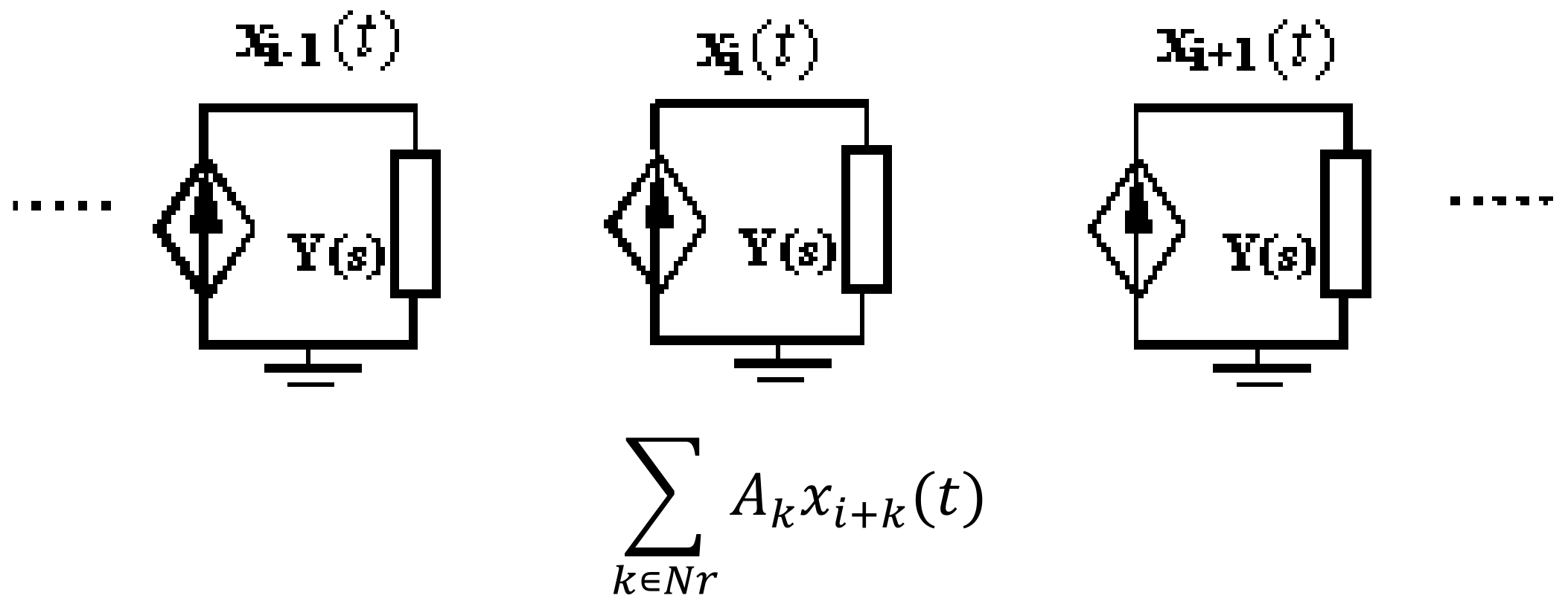
Another architecture studied systematically, both theoretically and regarding applications [5], is made of identical one-port cells characterized by an admittance Y(s), identically coupled by voltage-controlled current sources in a specified neighborhood with the A-template (and B-template if the array is nonautonomous), as sketched in Figure 4.

This case can also be analytically studied based on the cells and template homogeneities. In what follows, the decoupling techniques for a 1D autonomous case is presented.

In these conditions, the array output is the vector of voltages x_i(t) over the admittances Y(s) considered as linear integral-differential operators of the form:

$$Y\left(s\right)=\frac{Q\left(s\right)}{P\left(s\right)}=\frac{{{\displaystyle \sum }}_{l=0}^q{q}_l{s}^l}{{{\displaystyle \sum }}_{n=0}^p{p}_n{s}^n}$$

(7)

where $Q\left(s\right)$ and $P\left(s\right)$ are polynomials in the variable s↔d/dt.

The equations, in symbolic form, are:

$$Y\left(s\right)x\left(t\right)={{\displaystyle \sum }}_{k\in Nr}{A}_k{x}_{i+k}\left(t\right)$$

(8)

where Nr is the neighborhood of the A template, associated with the way the cells interact among them, the system being autonomous, i.e., the dynamics is produced be the nonzero state of the cells.

In these conditions, the above set of coupled equations can be solved by a similar decoupling technique, i.e., the change in variables:

$$x_i\left(t\right)={{\displaystyle \sum }}_{m=0}^{M-1}{\Phi }_M\left(i,m\right){\widehat{x}}_m\left(t\right)$$

(9)

where, for symmetric templates, the M functions ${\Phi }_M\left(i,m\right)$ are orthogonal with respect to the scalar product in C^M, so that ${\widehat{x}}_m$ can be expressed, by means of the inversion formulas, where:

$${\widehat{x}}_m\left(t\right)={{\displaystyle \sum }}_{i=0}^{M-1}{\Phi }_M^{*}\left(m,i\right)x_i\left(t\right)m=0,\dots ,M-1$$

(10)

$${\Phi }_M\left(m,i\right)={\Phi }_M^{*}\left(i,m\right)$$

(11)

For ring-type boundary conditions, Φ_M(m,i) have a similar form to that used in the two-grid coupled architecture, i.e., ${\Phi }_M\left(i,m\right)=e^{\mathrm{j}2\pi mi/M}=e^{j{\omega }_{m}i}{=\mathrm{e}}^{j{\omega }_{0}mi}$, where ω₀ = 2+π/M and ωm = 2πm/M = ω₀m, so that ${\Phi }_M\left(i+k,m\right)=e^{\mathrm{j}2\pi mk/M}{\Phi }_M\left(i,m\right)$. Thus, the action of the operators A on ${\Phi }_M\left(i,m\right)$ gives:

$${{\displaystyle \sum }}_{k\in Nr}{A}_k{\Phi }_M\left(i+k,m\right)=K_A\left(m\right){\Phi }_M\left(i,m\right)$$

(12)

Therefore, ${\Phi }_M\left(i,m\right)$ are eigenfunctions of the spatial operators represented by the A templates, and K_A(m) are the corresponding eigenvalues which, for symmetric templates A_-k = A_k, are real:

$$K_A\left(m\right)=A_0+2{{\displaystyle \sum }}_{k=1}^r{A}_k\cos \frac{2\pi mk}{M}$$

(13)

In particular, for r = 1 and r = 2, they have the form

$$K_A\left(m\right)=A_0+2A_1\cos \omega \left(m\right)=A_0+2A_1\cos \frac{2\pi }{M}m$$

(14)

and

$$K_A\left(m\right)=A_0+2A_1\cos \omega \left(m\right)+2A_2\cos 2\omega \left(m\right)=A_0+2A_1\cos \frac{2\pi }{M}m+2A_2\cos \frac{4\pi }{M}m$$

(15)

respectively.

Using the above change in variable, Equation (8) becomes, in symbolic form,

$$Y\left(s\right){\widehat{x}}_m\left(t\right)=K_A\left(m\right){\widehat{x}}_m\left(t\right)$$

(16)

or

$$Q\left(s\right){\widehat{x}}_m\left(t\right)=K_A\left(m\right)P\left(s\right){\widehat{x}}_m\left(t\right)$$

(17)

representing the differential equation satisfied by the amplitudes of the spatial modes of the array signals with respect to ${\Phi }_M\left(i,m\right)=e^{\mathrm{j}2\pi mi/M}$. The stability of each spatial mode depends on the characteristic equation associated with that particular mode. Thus, the characteristic polynomial associated with the m-th mode is:

$$R\left(s\right)=Q\left(s\right)-K_A\left(m\right)P\left(s\right)$$

(18)

showing how the dynamics of the spatial modes are determined by A and Y(s) = Q(s)/P(s), as presented in [5].

For the case Y(s) = Cs, the following first-order differential equations are obtained:

$$C\frac{d{\widehat{x}}_m\left(t\right)}{dt}=K_A\left(m\right){\widehat{x}}_m\left(t\right) m=0,\dots ,M-1$$

(19)

so that the characteristic equations roots are s_m = K_A(m)/C.

Similarly, for Y(s) = Cs + G, the relation becomes:

$$C\frac{d{\widehat{x}}_m\left(t\right)}{dt}=\left(-G+K_A\left(m\right)\right){\widehat{x}}_m\left(t\right)m=0,\dots ,M-1$$

(20)

with the roots s_m = (−G+K_A(m))/C. In both cases, K_A(m) is given by Equations (14) and (15) for first- and second-order neighborhoods, respectively.

Thus, the modes associated with roots with positive real parts will increase in time until signals will be limited by nonlinearities or by appropriate switches.

An example of a dispersion curve is given in Figure 5.

4. The Graph Y(s) Architecture

A further generalization of the above architecture has been made in [6,7,8] inspired by the works in [9,10] regarding the consensus in negative weights graph Laplacians and [11,12], where applications to graph-type circuit dynamics are discussed. As it is well-known, an undirected graph is a structure consisting of vertices interconnected by edges characterized by weights reflecting the relationship/interaction between cells placed in the vertices. The concept appears in many domains, including circuit theory. Thus, as shown in [11], there are still enough potential research subjects “at the intersection of algebraic graph theory and electrical networks”. The motivating aspects for dealing with the above-discussed subjects were the examples in Figures 1 and 2 in [11] representing a configuration formed by identical tank circuits grounded on one end and connected through identical resistors at the other end and, respectively, a transient showing synchronization of the node voltages. The architecture resembles that which was studied in [5], which consists of grounded cells described by identical admittances interconnected through voltage-controlled sources (that can be replaced by resistors in the symmetric case of the template). Related to the above architecture is that studied in [9] with respect to the consensus problem in the case of negative weighted graph branches (resistors).

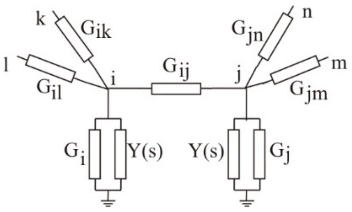
5. The Grounded Laplacian Y(s) Architecture

The graph neural structure studied next in this paper (Figure 6), which shall be called grounded Laplacian Y(s) architecture, has been analyzed in [8], the main focus being on the way the initial conditions influence the emergence of patterns due to unstable spatial modes and appropriate initial conditions. It is well-known that the genuine Laplacian (G_i = 0 for all i in Figure 6) associated with an undirected graph with positive weights is symmetric and has real and positive eigenvalues. Thus, the only way unstable modes can be obtained in architectures associated with a graph Laplacian is based on the active character of the cells. On the other hand, since any symmetric matrix has real eigenvalues and orthogonal eigenvectors, the most convenient architecture that avoids active cells at the price of allowing negative weights, as well as grounded edges, is that presented in Figure 6.

In the following, the results reported in [7,8] will be briefly presented. As shown above, in the architecture (positive or negative) edges/resistances in parallel to the admittances are allowed, connecting nodes to ground. Thus, the two aspects that make the architecture theoretically tractable are (a) the nondirected resistive branches (including grounded ones) and (b) identical grounded admittances. The first condition ensures the symmetric character of the interconnection matrix which means real eigenvalues and orthogonal eigenvectors, and the second, the possibility of studying the dynamics using similar equations in the amplitudes of the spatial modes of the network. The specific characteristic of the architecture is that, in the general case, the eigenvalues and eigenvectors of the interconnection matrix cannot be expressed analytically.

As shown in [8], the nodal equations are:

$$Y\left(s\right)\left[V\left(s\right)\right]+\left[G\right]\left[V\left(s\right)\right]=\left[J\left(s\right)\right]$$

(21)

where

$$\left[G\right]=\left[\begin{array}{c}{G}_{11}{G}_{12}\dots G_{1M}\\ ⋮⋮⋮\\ G_{M1}{G}_{M2}\dots G_{MM}\end{array}\right]$$

(22)

is the matrix characterizing the resistive graph with G_ij = G_ji (i.e., symmetric with real eigenvalues and orthogonal eigenvectors), and [V(s)] and [J(s)] are vectors denoting, respectively, the nodal voltages and the equivalent current sources determined by the initial condition in the admittances Y(s).

In Ref. [8], the general case for initial conditions different from the nodal voltages has been considered by using their spectral decomposition and the equivalent current sources as linear combinations of the above spectra. With the notations [J(s)] = [X][A(s)], the equations in the Laplace domain that describe the system evolution due to initial conditions are:

$$Y\left(s\right)\left[V\left(s\right)\right]+\left[G\right]\left[V\left(s\right)\right]=\left[X\right]\left[A\left(s\right)\right]$$

(23)

where [X] is the matrix of the initial conditions (with dimension M × N), A(s) of dimension 1 × N is the matrix that converts the initial conditions into current sources injecting charge into the nodes, and M and N are the number of nodes and the degree of Y(s), respectively.

Represented by [Φ], the M × M matrix of the eigenvectors of [G], by $[\widehat{V\left(s\right)}]$ and $[\widehat{X}]$ the spectra of [V(s)] and [X] with respect to the system eigenvectors, the node voltages and the initial conditions become $\left[V\right]=\left[\Phi \right][\widehat{V}]$ and $\left[X\right]=\left[\Phi \right][\widehat{X}]$, respectively, so that (23) can be written as:

$$Y\left(s\right)\left[\Phi \right][\widehat{V\left(s\right)}]+\left[G\right]\left[\Phi \right][\widehat{V\left(s\right)}]=\left[\Phi \right][\widehat{X}]\left[A\left(s\right)\right]$$

(24)

Multiplying the above equations with ${\left[\Phi \right]}^{\mathrm{T}}$ and taking advantage of the orthogonality, one obtains:

$$Y\left(s\right)[\widehat{V\left(s\right)}]+\left[\lambda \right][\widehat{V\left(s\right)}]=[\widehat{X}]\left[A\left(s\right)\right]$$

(25)

where $\left[\lambda \right]$ is the diagonal matrix composed of the system eigenvalues.

Thus, the above system contains decoupled equations of the form:

$$Y\left(s\right){\widehat{v}}_m\left(s\right)+{\lambda }_m{\widehat{v}}_m\left(s\right)=\left[{\widehat{x}}_{m,1},\cdots ,{\widehat{x}}_{m,N}\right]\left[A\left(s\right)\right]$$

(26)

for each (spatial) mode m of the interconnection matrix.

Considering again admittances Y(s) of the form (7):

$$Y\left(s\right)=\frac{Q\left(s\right)}{P\left(s\right)}$$

the equations that describe the dynamic of the modes are:

$$Q\left(s\right){\widehat{v}}_m\left(s\right)+{\lambda }_{m}P\left(s\right){\widehat{v}}_m\left(s\right)=P\left(s\right)\left[{\widehat{x}}_{m,1},\cdots ,{\widehat{x}}_{m,N}\right]\left[A\left(s\right)\right]$$

(27)

with the symbolic form solution:

$${\widehat{v}}_m\left(s\right)=\frac{P\left(s\right)\left[{\widehat{x}}_{m,1},\cdots ,{\widehat{x}}_{m,N}\right]\left[A\left(s\right)\right]}{Q\left(s\right)+{\lambda }_{m}P\left(s\right)}$$

(28)

Since A(s) has poles in the left half-plane for a passive Y(s), the above expression shows that the unstable spatial modes m are those for which the polynomial $Q\left(s\right)+{\lambda }_{m}P\left(s\right)=0$ is not Hurwitz. In fact, the dynamics and stability of each spatial mode is determined by the roots of this polynomial for all λ_m. This observation led to the idea of using the root locus approach to appreciate the spatial modes stability discussed in [8]. Moreover, the unstable mode(s) will develop/increase only if it (they) exists in at least one initial condition. In such a case, the signals will grow until reaching a nonlinearity or being stopped by appropriate switches.

6. Synthesis of Networks with Prescribed Unstable Spatial Modes

In this section, the idea of synthesizing graph-type networks of the form discussed above with imposed spatial modes and dynamics exhibiting unstable modes is analyzed. An important aspect is the fact that symmetric matrices have orthogonal eigenvectors and, moreover, that it is possible to synthesize matrices with imposed eigenvectors and associated eigenvalues [13]. In principle, for a given set of orthogonal vectors, part of them can be associated with positive eigenvalues, and the other part with negative ones, implying a possible competition of the unstable modes. In fact, the simplest case, for a specified set of orthogonal eigenvectors, is to adopt a positive eigenvalue for one of them and negative ones for the rest of them. The “unstable” vectors correspond to a bundle [14] associated to the “stable” vectors decided to be related to negative eigenvalues. In the examples that follow, only the case of one unstable spatial mode is considered, and all other modes diminish with time.

As already mentioned, the essence of pattern formation in a grounded Laplacian Y(s) structure is the existence of (at least) one eigenvalue, which makes the polynomial $Q\left(s\right)+{\lambda }_{m}P\left(s\right)=0$ non-Hurwitz.

A remarkable aspect is that, if the interest is only in the “polarity” of an unstable mode, no matter how small, “hidden” in the initial conditions, the network will permit detection according to the pattern developed during the transience. The small deviations in the eigenvectors form their ideal values and will not change their stability or instability. Thus, the unstable character of one or several eigenvectors will remain unchanged, and, for the latter case, the result of a mode competition will determine the “winning” mode according to the weights of the unstable modes as well as to the values of the r.h.p eigenvalues.

Regarding the above considerations, an obvious concern is that of how the precision the parameters of the cells and the interconnecting graph should be ensured for a physical implementation. Fortunately, a remarkable theorem put forth by Ostrowski [15], stating that the eigenvalues of a matrix are continuous functions of its entries, ensures that small deviations in the matrix entries will not change the side of the complex plane position of the eigenvalues. Moreover, for small deviations from the nominal values, it is expected that the eigenvectors do not change significantly, as long as the matrices do not have large condition numbers. Another possibility to determine the sign of a component in a given/prescribed orthogonal base could consist of taking the scalar product of the initial conditions signal and the component whose sign or perhaps amplitude of interest. However, the presented solution is completely analog, i.e., does not require A/D conversion and scalar product computation being based on unstable spatial modes.

7. Proof of Concept: Towards a Spatial Modes Comparator (Detecting Sign of “Hidden” Spatial Mode)

In what follows, a toy example is presented as a proof of concept illustrated both for a positive and negative resistor graph-like circuit realization, as well as for a CMOS transistor (active) one. This example has adopted the eigenvector v = [1 −1 1 −1]^T associated with the eigenvalue −2 which, in the nodal equations, will correspond to a positive eigenvalue, i.e., +2. For simplicity, the admittance Y(s) is that of an ideal capacitor, i.e., Y(s) = Cs. According to [14], for M = 4, three self-orthogonal vectors and orthogonal on a vector [a b c d]^T are [−b a −d c]^T, [−c d a −b]^T and [−d −c b a]^T. Thus, for a = 1, b = −1, c = 1 and d = −1, associating the eigenvalue -2 for the first and +2 for the other three eigenvectors, we have the following pairs eigenvalue-eigenvector:

−2 [1 −1 1 −1]^T

2 [1 1 1 1]^T

2 [−1 −1 1 1]^T

2 [1 −1 −1 1]^T

Using [13], the graph/nodal matrix is:

$$G=\left[\begin{array}{c} 1 1-1 1 \\ 1 1 1-1\\ -1 1 1 1\\ 1-1 1 1\end{array}\right]$$

The circuit schematic for Y(s) = Cs described by the nodal equations (particular case of (23)):

$$sC\left[V\left(s\right)\right]+\left[G\right]\left[V\left(s\right)\right]=C\left[V\left(0\right)\right]$$

associated with the matrix G above is presented in Figure 7, where the resistances have been adopted in the order of hundreds of KOhms and capacitors 10 pF; to limit nodal voltages, antiparallel diodes have been connected between each node and the ground. For the linear operation, the spatio-temporal dynamics are governed by the eigenvalues 2, −2, −2, −2, and the unstable spatial mode [1 −1 1 −1]^T associated with the root s = +2 and the stable ones, [1 1 1 1]^T, [−1 −1 1 1]^T and [1 −1 −1 1]^T, are all associated with the same root s = −2.

The circuit in Figure 7 has been also analyzed replacing the “classical” resistors by floating active (simulated in CMOS technology with CMOS versions of bipolar realizations in [16]) positive and negative resistors with the schematics shown in Figure 8. The node numbering is the same for both realizations, i.e., that of Figure 7. In the following, several examples (with resistors and simulated resistors) regarding the way the initial conditions (voltages on the vertices/grounded capacitors) determine the dynamics of the spatial modes are presented. The simulations have been performed in the Cadence environment (0.180 u technology). All transistor sizes were l = 1.80 u, w = 0.5 u.

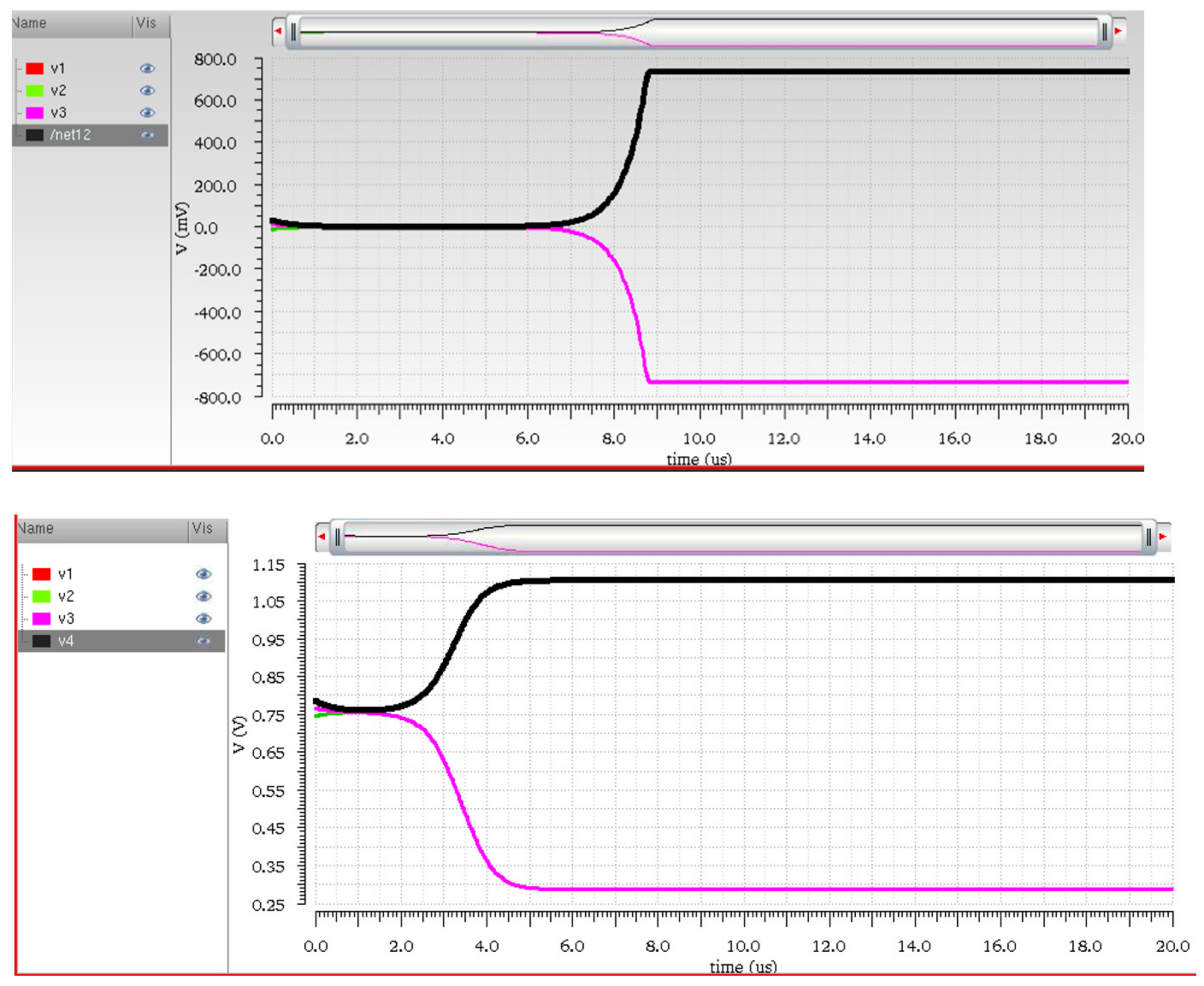
The first example (Figure 9) considers the initial conditions [v1(0) v2(0) v3(0) v4(0)]^T = [1 µV −1 µV 1 µV −1 µV]^T (the unstable mode with a very small positive amplitude) seeded on the four capacitors. It can be seen that in both realizations, the mode develops until the nonlinearities limit the voltage increase (v1—red; v3—magenta) or decrease (v2—green; v4—black).

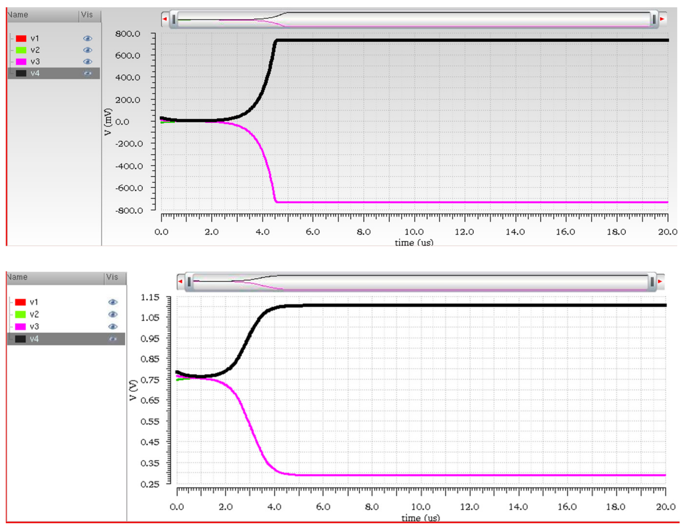
For the next simulations (Figure 10), the sign of the (same unstable) mode seeded as initial conditions have been changed, i.e., [v1(0) v2(0) v3(0) v4(0)]^T = [−1 µV 1 µV −1 µV 1 µV]^T. It can be seen that in both cases the final pattern is the opposite from the previous one (Figure 10). Now the voltages v1—red—and v3—magenta—have decreased, while v2—green—and v4—black—increased.

A second example corresponds to initial conditions [10 mV 10 mV 10 mV 10 mV]^T proportional to the first stable eigenvector. In the first part, the dynamics are stable and end in instability due to the numeric noise, as seen in Figure 11.

The next simulations shown in Figure 12, correspond to initial conditions [v1(0) v2(0) v3(0) v4(0)]^T = [10 mV −10 mV 10 mV 30 mV]^T, i.e., proportional to the sum of the three stable modes.

Observe that due to nonlinearities and computational noise, after a while, the unstable mode develops with positive weight.

Added to the above initial conditions is 2% of the unstable mode so that they become [10.2 mV −10.2 mV 10.2 mV 29.8 mV]^T. Observe (Figure 13) that the “hidden” unstable mode develops with positive amplitude.

Next, (Figure 14) the initial conditions are [9.8 mV −9.8 mV 9.8 mV 30.2 mV]^T, obtained by subtracting 2% of the unstable mode from those in Figure 12.

Observe that the unstable mode has developed with opposite polarity in both cases. It follows that, at least within certain conditions regarding the range of amplitudes, the discussed architecture is able to detect the sign of a small hidden mode that has been designed to be unstable. When more unstable modes coexist, there will be a mode competition, the winning mode being determined by the amplitude of the unstable modes in the initial conditions and the values of their associated eigenvalues. Indeed, the dynamics might be influenced by the nonlinearities used to limit the growth of the unstable mode(s). Thus, the coincidence between theoretical and experimental realizations regarding a specific neural/graph architecture with a possible application of detecting the sign of certain hidden modes used in the design of the network is illustrated.

8. Concluding Remarks

The dynamics and principle of pattern formation in a couple of classes of cellular and graph neural circuits have been presented and discussed, emphasizing the common characteristics of all realizations, i.e., the existence of unstable spatial modes. The way in which analytical solutions can be obtained by using the decoupling technique, based on the orthogonality of the spatial modes, has been illustrated. For each case, there has been a brief outline of the way the equations can be decoupled using the amplitudes of the modes as the new dynamical variables. In addition to these theoretical aspects, in the last part, as a proof of concept, an example showing the possibility of identifying a “hidden” unstable mode by designing a graph neural circuit with prescribed eigenvalues and eigenvectors has been presented. Thus, it has been proven that circuits with prescribed eigenvectors and eigenvalues can be designed to detect the presence and the sign of a small unstable mode among the other stable ones. Simulations including a CMOS realization confirmed the analytical results; of course, the author is aware of the limitations due to parasites and tolerances, which might restrict the range of signal variation. However, the presented proof of concept shows how the subject of pattern formation could be associated to the design of what has been called a spatial comparator.

References

- Turing, A.M. The Chemical Basis of Morphogenesis. Phil. Trans. R. Soc. Lond. B 1952, 237, 37–72. [Google Scholar]
- Chua, L.O.; Yang, L. Cellular Neural Networks: Theory. IEEE Trans. Circuits Syst. 1988, 35, 1257–1272. [Google Scholar] [CrossRef]
- Chua, L.O.; Yang, L. Cellular Neural Networks: Applications. IEEE Trans. Circuits Syst. 1998, 35, 1273–1290. [Google Scholar] [CrossRef]
- Goraş, L.; Chua, L.O. Turing Patterns in CNN’s-Part II: Equations and Behaviors. IEEE Trans. Circuits Syst. 1995, 42, 612–626. [Google Scholar] [CrossRef]
- Goras, L.; Vornicu, I.; Ungureanu, P. Topics on Cellular Neural networks. In Handbook on Neural Information Processing; Bianchini, M., Maggini, M., Jain, L., Eds.; Springer: Berlin/Heidelberg, Germany, 2013; pp. 97–141. [Google Scholar]
- Goras, L.; Fira, M. On Signal Processing on Graphs, Patterns, Consensus and Manifolds. J. Eng. Sci. Innov. 2018, 3, 291–298. [Google Scholar]
- Goras, L.; Savinescu, V.S.; Nica, I. On Pattern Formation in Homogeneous and Nonhomogeneous Cellular Neural Networks. In Proceedings of the 14-th Symposium on Neural Networks and Applications (NEUREL), Belgrade, Serbia, 20–21 November 2018. [Google Scholar]
- Goraş, L.; Ungureanu, P.; Fira, M. On Pattern Formation in a Class of Graph Neural Networks. In Proceedings of the 2021 International Symposium on Signals, Circuits and Systems (ISSCS), Iasi, Romania, 15–16 July 2021; pp. 1–5. [Google Scholar] [CrossRef]
- Zelazo, D.; Bürger, M. On the definiteness of the weighted Laplacian and its connection to effective resistance. In Proceedings of the 53rd IEEE Conference on Decision and Control, Los Angeles, CA, USA, 15–17 December 2014; pp. 2895–2900. [Google Scholar] [CrossRef]
- Chen, Y.; Khong, S.Z.; Georgiou, T.T. On the definiteness of graph Laplacians with negative weights: Geometrical and passivity-based approaches. In Proceedings of the 2016 American Control Conference (ACC), Boston, MA, USA, 6–8 July 2016; pp. 2488–2493. [Google Scholar] [CrossRef]
- Dörfler, F.; Simpson-Porco, J.W.; Bullo, F. Electrical Networks and Algebraic Graph Theory: Models, Properties, and Applications. Proc. IEEE 2018, 106, 977–1005. [Google Scholar] [CrossRef]
- Daković, M.; Stanković, L.; Lutovac, B.; Sejdić, E.; Šekara, T.B. A resistive circuits analysis using graph spectral decomposition. In Proceedings of the 2017 6th Mediterranean Conference on Embedded Computing (MECO), Bar, Montenegro, 11–15 June 2017; pp. 1–4. [Google Scholar] [CrossRef]
- Arndt Brünner. Available online: https://www.arndt-bruenner.de/mathe/scripts/engl_eigenwert2.htm (accessed on 10 March 2021).
- Generate a Set of Orthogonal Vectors to a Given Vector. Available online: https://scicomp.stackexchange.com/questions/27834/generate-a-set-of-orthogonal-vectors-to-a-given-vector (accessed on 15 March 2021).
- Ostrowski, A. Sur la continuité relative des racines d’équations algébriques. Acad. Sci. Paris Compt. Rendus 1939, 209, 777–779. [Google Scholar]
- Tekin, A.S.; Alçı, M. Design and Applications of Electronically Tunable Floating Resistor Using Differential Amplifier. Elektron. Ir Elektrotechnika 2013, 19, 41–46. [Google Scholar] [CrossRef]
Figure 1.
Cell, symbol and sketch of a 1D array for the two-grid coupled architecture.
Figure 2.
Dispersion curve showing possible pattern generation.
Figure 3.
Mode competition for the u voltages in Figure 1a in a 30 cell 1D array.
Figure 4.
Sketch of 1D Y(s) architecture.
Figure 5.
Example of a dispersion curve for a band-pass spatial filter (pass band/unstable modes region marked with thick line).
Figure 6.
Sketch of grounded Laplacian Y(s) architecture.
Figure 7.
Schematic corresponding to the network example with imposed eigenvectors and eigenvalues and limitation of signals with antiparallel diodes.
Figure 8.
Floating positive (a) and negative (b) resistor used in active simulation of circuit in Figure 7.
Figure 9.
Transient from initial conditions [v1 v2 v3 v4]T = [1 µV −1 µV 1 µV −1 µV]T for the two realizations.
Figure 10.
Transient from initial conditions [v1(0) v2(0) v3(0) v4(0)]T = [−1 µV 1 µV −1 µV 1 µV]T for the two realizations.
Figure 11.
Transient from initial conditions [v1(0) v2(0) v3(0) v4(0)]T = [10 mV 10 mV 10 mV 10 mV]T for the two realizations.
Figure 12.
Transient from initial conditions [v1(0) v2(0) v3(0) v4(0)]T = [10 mV −10 mV 10 mV 30 mV]T for the two realizations.
Figure 13.
Transient from initial conditions [v1(0) v2(0) v3(0) v4(0)]T = [10.2 mV −10.2 mV 10.2 mV 29.8 mV]T for the two realizations.
Figure 14.
Transient from initial conditions [v1(0) v2(0) v3(0) v4(0)]T = [9.8 mV −9.8 mV 9.8 mV 30.2 mV]T for the two realizations.
Publisher’s Note: MDPI stays neutral with regard to jurisdictional claims in published maps and institutional affiliations. |
© 2022 by the author. Licensee MDPI, Basel, Switzerland. This article is an open access article distributed under the terms and conditions of the Creative Commons Attribution (CC BY) license (https://creativecommons.org/licenses/by/4.0/).
Share and Cite
MDPI and ACS Style
Goras, L. On Unstable Spatial Modes and Patterns in Cellular and Graph Neural Circuits. Electronics 2022, 11, 3033. https://doi.org/10.3390/electronics11193033
AMA Style
Goras L. On Unstable Spatial Modes and Patterns in Cellular and Graph Neural Circuits. Electronics. 2022; 11(19):3033. https://doi.org/10.3390/electronics11193033
Chicago/Turabian StyleGoras, Liviu. 2022. "On Unstable Spatial Modes and Patterns in Cellular and Graph Neural Circuits" Electronics 11, no. 19: 3033. https://doi.org/10.3390/electronics11193033
Note that from the first issue of 2016, this journal uses article numbers instead of page numbers. See further details here.