Systematic Comparison of Objects Classification Methods Based on ALS and Optical Remote Sensing Images in Urban Areas

Abstract

Geographical object classification and information extraction is an important topic for the construction of 3D virtual reality and digital twin cities in urban areas. However, the majority of current multi-target classification of urban scenes uses only a single source data (optical remote sensing images or airborne laser scanning (ALS) point clouds), which is limited by the restricted information of the data source itself. In order to make full use of the information carried by multiple data sources, we often need to set more parameters as well as algorithmic steps. To address the above issues, we compared and analyzed the object classification methods based on data fusion of airborne LiDAR point clouds and optical remote sensing images, systematically. Firstly, the features were extracted and determined from airborne LiDAR point clouds and high-resolution optical images. Then, some key feature sets were selected and were composed of median absolute deviation of elevation, normalized elevation values, texture features, normal vectors, etc. The feature sets were fed into various classifiers, such as random forest (RF), decision tree (DT), and support vector machines (SVM). Thirdly, the suitable feature sets with appropriate dimensionality were composed, and the point clouds were classified into four categories, such as trees (Tr), houses and buildings (Ho), low-growing vegetation (Gr), and impervious surfaces (Is). Finally, the single data source and multiple data sources, the crucial feature sets and their roles, and the resultant accuracy of different classifier models were compared and analyzed. Under the conditions of different experimental regions, sampling proportion parameters and machine learning models, the results showed that: (1) the overall classification accuracy obtained by the feature-level data fusion method was 76.2% compared with the results of only a single data source, which could improve the overall classification accuracy by more than 2%; (2) the accuracy of the four classes in the urban scenes can reach 88.5% (Is), 76.7% (Gr), 87.2% (Tr), and 88.3% (Ho), respectively, while the overall classification accuracy can reach 87.6% with optimal sampling parameters and random forest classifiers; (3) the RF classifier outperforms DT and SVM for the same sample conditions. In this paper, the method based on ALS point clouds and image data fusion can accurately classify multiple targets in urban scenes, which can provide technical support for 3D scene reconstruction and digital twin cities in complex geospatial environments.

1. Introduction

For the needs of urban 3D (three dimensional) scene modeling, digital twin city and urban resource management, the accurate classification and extraction of feature objects in urban areas is a key issue that needs to be addressed urgently. Airborne LiDAR (Light Detection And Ranging) technology is widely used in the military, agriculture, mapping, and other fields [1], and can directly and quickly obtain high-precision 3D information on surface objects in urban areas, which has become an important remote sensing data source and is now widely used in the fields of urban 3D reconstruction and urban road detection and planning [2,3,4,5]. Remote sensing image data are also an important data source for feature classification and extraction, and many scholars use images for building and road extraction [6,7,8].

However, the current objective classification in urban scenes usually uses a single data source or homogenous data, which has the advantage that the homogenous data have the same information storage structure and can be fused with the source data during the data pre-processing stage. However, urban areas are usually a complex and dynamic environment, and this complexity makes it difficult to meet all the requirements of a single sensor in remote sensing data for urban applications [9]. Therefore, a single sensor is not sufficient to provide all the important information regarding feature extraction and classification purposes [10]. Some scholars just extract features from LiDAR data: for example, Song et al. [11] describe a study which evaluated the utilization of LiDAR data in land cover classification. By transforming the point cloud into a grid format and categorizing the intensity data obtained into four groups—grass, trees, asphalt pavement, and house roofs—this method’s key is to identify objects based on reflection intensity. Bellakaout et al. [12] mentioned a classification method that uses a single-echo LIDAR for contour identification of ground objects: upper contour, lower contour, uniform, and non-uniform surfaces, which in turn extracts soil, vegetation, buildings and roads. Zhang et al. [13] used a surface growth method to cluster point cloud data, object-oriented construction of feature vectors, and classification of point clouds based on SVM (support vector machine).

Through the above-mentioned scholars’ studies, it is easy to find that, due to the complexity of airborne LiDAR point cloud data due to its scene and irregular spatial distribution, segmentation and classification using only LiDAR data in multi-objective classification in urban areas are prone to misclassification, which can lead to problems such as features that are similar in 3D morphology not being identified. In order to obtain more accurate objective classification results, these scholars usually optimize their algorithms or design more complex algorithms based on the actual data, which is the limitation of a single data source. Therefore, some scholars classify point cloud data or remote sensing image data with the aid of other data sources. Zhou et al. [14] used super voxels as the basic unit to fuse airborne LiDAR point clouds and DIM (digital intensity models) point clouds at the feature level using different weights, and used an improved binary TrAdaboost classifier to classify the point clouds into three categories: building, ground, and vegetation. Guo et al. [15] proposed a multi-source framework by combining multi-echo LiDAR data, full-waveform LiDAR data and multispectral image data to classify dense urban areas. Su et al. [16] extracted the elevation information from LiDAR data to participate and assist in urban land cover classification from remote sensing images, which effectively increased the production accuracy of buildings. Cheng et al. [17] used spectral information to first separate vegetation and then elevation information to separate surface roads and buildings. Suarez et al. [18] investigated the combined use of aerial photography and airborne LiDAR for more accurate classification and tree height estimation in forestry. Wang and Li. [19] used the density of corner points (DCP) in spectral images to quantify spatial features, dual-time very high resolution (VHR) satellite data and airborne LiDAR data to generate dual-time height and corner features, and combined both data to assess building damage after a disaster. Awrangjeb et al. [20] used color and texture information to classify point clouds into broad categories by effectively integrating LiDAR data and multispectral orthophotos, and then achieved automatic extraction of building roofs by area growth. S. Y. Sadjadi and S. Persian [21] used machine learning algorithms for HS- and LiDAR-fused data to achieve accurate extraction of buildings at the pixel level. In addition, it has been shown in the studies of many scholars that the classification accuracy of features can be effectively improved by using methods that fuse different data [22,23,24,25]. However, most of the above scholars’ ways of utilizing multi-source data are to first filter one kind of data based on some unique information (color information of images or elevation information of point cloud data, etc.) of another kind of data, and then classify the filtered data into objectives, and they do not make full use of the differences between the information of multi-source data.

To make fuller use of the information from multiple sources to improve the accuracy of objective classification, scholars often choose machine learning or deep learning methods; the difficulty of deep learning lies in the adjustment of numerous parameters and the time consumption required to train them and the need for high-end hardware platform support, so this paper chooses the more efficient and convenient machine learning method. In terms of which machine learning classifier to choose, scholars often need to choose the type of classifier according to the actual situation. Currently, the use of 3D point clouds for urban remote sensing information extraction using machine learning methods has become a popular area of research, which can use the features extracted from 3D point clouds for automatic learning of mathematical models and rely on feature information to effectively discriminate or classify different objects in complex urban areas. In terms of the use of machine models, different scholars have chosen different classifier methods including DT (decision tree), RF (random forest), SVM, XGBoost (eXtreme gradient boosting) [26,27,28,29,30], etc. Du et al. [31] extract building classes and vehicle classes in urban areas by DT model, but it requires manual setting of constraints on the features and has certain requirements on point cloud density and area topography. Sukhanov et al. [18] present an ensemble-based approach based on MS (multi-spectra), LiDAR, HS (high-spectra), and RGB imagery for urban land use and land cover classification. This approach contains RF and Gradient Boosting Machine (GBM) classifiers and convolutional neural networks (CNNs). Xu et al. [32] converted LiDAR point clouds into 2D raster data and combined them with image data to extract various features for classification objects and selected a SVM classifier for urban feature classification. Dong. [33] introduced SVM into point cloud and image fusion classification to effectively reduce the misclassification rate of trees and buildings. Hamid et al. [34] used the Improved Vector Machine for the classification of clustered bodies. Based on LiDAR point cloud data and color information of the images, Hu et al. [35] classified the point clouds using a random forest model through a method based on fusion of multi-basis element feature vectors. However, the above-mentioned scholars’ studies generally only focus on single or two terrain targets for classification extraction, while for the processing of multiple terrain targets, the selection and combination of features often needs to be optimized.

The classification performance of a classifier is limited by various aspects, and the selection and combination of features is the most critical part of it. The availability of many features (e.g., spectral, spatial, morphological, geometric, and textural features) makes the exact selection of features difficult. Second, too many feature dimensions make the training time of the classifier longer and may lead to dimensional disasters, so feature selection methods are necessary [36], and some scholars believe that a reasonable selection of fused features can provide better performance to the classifier [37]. Chehata et al. [38] summarized 21 common features of 3D point cloud data.

In summary, for the problem of how to improve the accuracy of multi-place object classification in urban scenes, in this study we used machine learning for classification to improve the classification extraction accuracy of urban scene objects based on airborne LiDAR point clouds and high-resolution optical remote sensing images by fusing the 2D spectral and textural information of images and 3D information and spatial structure information of point clouds through feature extraction. It also demonstrates the following points and objectives in this study through three aspects (data source, selection of feature set and classifier): (1) The superiority of multi-source data fusion compared to single-source data for the extraction of multi-object targets in urban scenes, (2) The importance of suitable classifiers, (3) The necessity of optimizing feature combinations; also, it analyzes the sampling ratio parameters as well as the classifier optimization parameters., aiming to provide a general and flexible framework for the multi-classification problem in urban scenes.

2. Materials and Methods

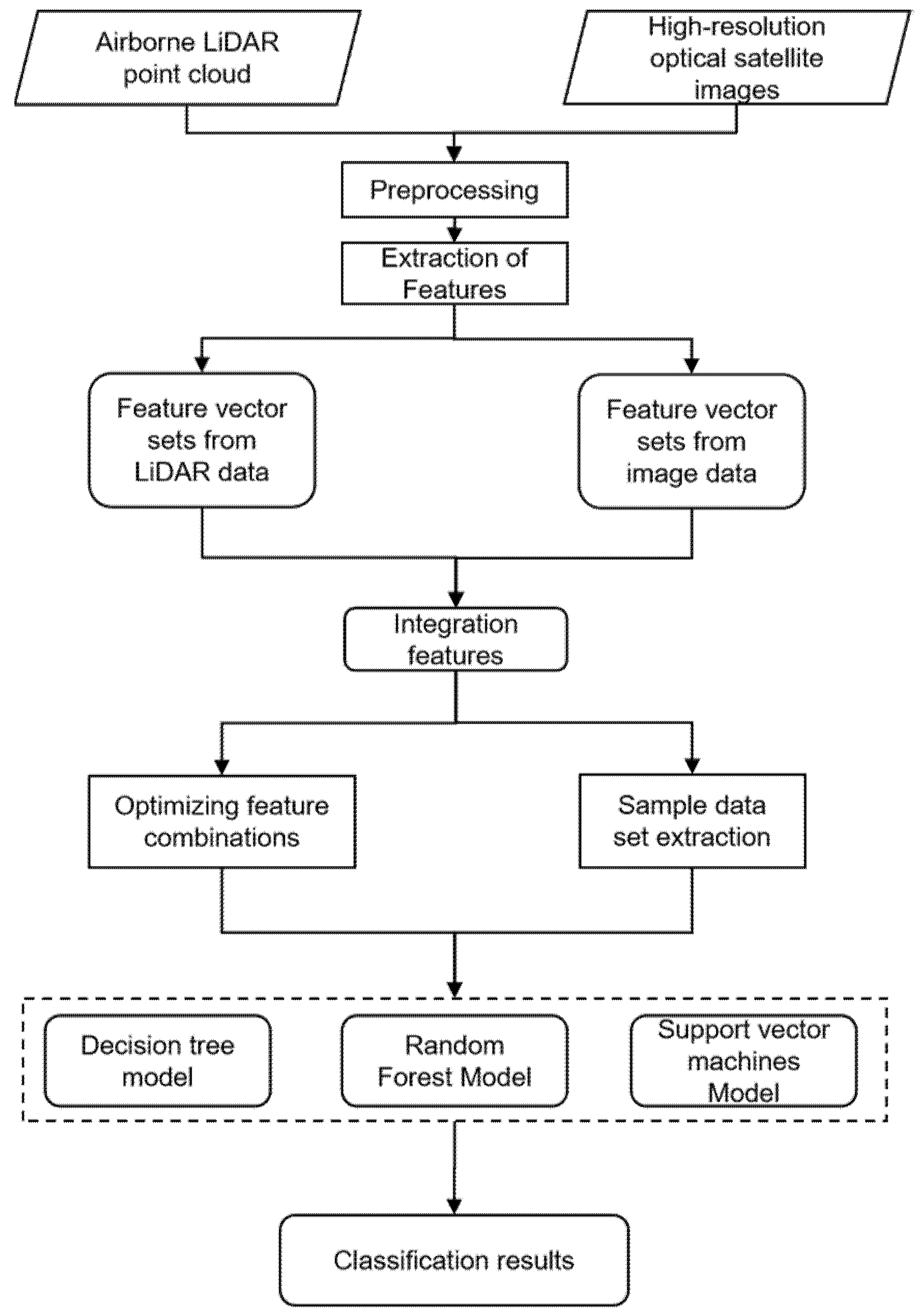
2.1. Technical Process

In this study, based on airborne LiDAR point cloud and high-resolution optical image data, we studied feature extraction and fusion of 2D–3D information for application to feature object classification extraction of complex urban areas. The technical route process of this paper mainly includes four main steps: extraction and fusion of features and construction of feature sets, optimization of feature combinations, extraction of samples, establishment of classification models and classification results. The detailed technical flowchart of this study is shown in Figure 1. It mainly includes: (1) Calculating the features of optical images and LiDAR point clouds, combining them into different feature sets, and comparing and analyzing the classification results of single-source and multi-source. (2) Optimizing the feature sets so that they can reduce time consumption while ensuring accuracy. (3) A certain sample size is taken as the input data of the machine learning model, and the sensitivity of the sampling proportion parameter is analyzed to further improve the classification accuracy. (4) To explore the effect of classifier selection on the classification results, experiments are conducted using different classifiers.

2.2. Feature Extraction and Fusion from Airborne LiDAR Point Clouds and Optical Images

In this study, feature extraction is performed for both airborne LiDAR point cloud and optical image data separately, and feature set F_1 is constructed in the form of point cloud features as the main feature and optical image features as the supplementary feature, i.e., the feature fusion process of the two data sources. In the feature set F_1, all of them are based on point neighborhood statistical features except for the normalized elevation features (Normalized Height,), intensity, normalized green-red difference index ($NGRDI$), and texture features. The calculation methods of each feature and their descriptions are shown in

Table 1. Statistical results of point cloud data information.

Features	Calculation Methods	Descriptions
Normalized elevation values	$N_h=H-H_{DTM}$	Elevation values of features after eliminating the effect of slope
Elevation Skewness	$H_{skw}=\frac{{{\displaystyle \sum }}_1^n{\left(N_{hi}-\overline{N_h}\right)}^3}{{[{{\displaystyle \sum }}_1^n{\left(N_{hi}-\overline{N_h}\right)}^3]}^{3/2}}$	Measure of the direction and degree of skewness of the distribution of elevation statistics
Elevation kurtosis	$H_{kur}=\frac{{{\displaystyle \sum }}_1^n{\left(N_{hi}-\overline{N_h}\right)}^4}{{[{{\displaystyle \sum }}_1^n{\left(N_{hi}-\overline{N_h}\right)}^3]}^2}$	A measure of outliers in elevation statistics
Absolute deviation of median elevation	$MAD\_1=median\left(\left|N_{hi}-median\left(N_h\right)\right|\right)$	Robust measures of sample variability in elevation statistics
Absolute deviation of mean elevation	$MAD\_2=median\left(\left|N_{hi}-\overline{N_h}\right|\right)$	Median of the difference between the midpoint of elevation statistics and the mean of elevation
Normalized Red-Green Difference Index	$NGRDI=\frac{G-R}{G+R}$	Indicators of vegetation and non-vegetation
Echo intensity value	$In$	Echo intensity value
The angle between the normal vector and the vertical direction	$S_n$	The angle between the normal vector and the vertical direction
Coefficient of variation of texture features	$GLCM\_V=\frac{{{\displaystyle \sum }}^{}{\left(p\left(n\right)-m\right)}^2}{n-1}$	M is the average DN value of the moving window
Texture feature angle second order moment	$GLCM\_ASM={\displaystyle {\displaystyle \sum }_i}{\displaystyle {\displaystyle \sum }_j}{[p\left(n\right)]}^2$	Describes the uniformity of image grayscale distribution and texture roughness
Texture feature information entropy	$GLCM\_ENT=-{\displaystyle {\displaystyle \sum }_i}{\displaystyle {\displaystyle \sum }_j}p\left(n\right)\log p\left(n\right)$	Expresses the amount of information the image has
Homogeneity of textural features	$GLCM\_H={\displaystyle {\displaystyle \sum }_i}{\displaystyle {\displaystyle \sum }_j}\left(\left(\frac{1}{1+{\left(i-j\right)}^2}\right)\frac{p\left(n\right)}{{{\displaystyle \sum }}_i{{\displaystyle \sum }}_{j}p\left(n\right)}\right)$	Intensity and amplitude of the continuous variation of the gray level of the image element and its neighbors

.

In Table 1, The DTM (Digital Terrain Model, DTM) in the normalized elevation feature formulation is constructed by the fabric simulation algorithm proposed by Zhang et al. [39]. The domain of points involves the nearest neighbor query, and the KD (K-dimension) tree [40,41] is used in this study to improve the search efficiency of the nearest neighbor points. Texture features are extracted by the Gray Level Co-occurrence Matrix (GLCM) method in this study. The concept of texture originates from the feedback of human skin to the smoothness and roughness of the object surface, and the Gray Level Co-occurrence Matrix is a classical statistical method to describe the texture of a region, and it is still widely used in the texture feature extraction of high-resolution remote sensing images; the size of the window to obtain the G Gray-level Co-occurrence Matrix is 5 × 5 pixels, the step size is 1, and the directions are selected as 0°, 45°, 90°, 135°; The average value of the four directions is taken as the value of the relevant feature, and if there is an infinite value, the window size is automatically expanded gradually until the feature value is a valid and normal value.

2.3. Feature Sets Selection and Determination by PCA and Artificial Knowledge

Five feature sets are created in this study using various strategies to examine the impact of various selection techniques on the overall classification accuracy. First, F_1 is the feature set created by combining all of the retrieved features. The feature set F_1 contains a total of 12 features: {$N_h$,$H_{skw}$,$H_{kur}$,$I_n$,$S_n$,$NGRDI$,$GLCM\_V$,$GLCM\_ASM$,$GLCM\_ENT$,$GLCM\_H$,$MAD\_1$,$MAD\_2$}. Combine the features extracted from the point cloud into feature set F_2: {$N_h$,$H_{skw}$,$H_{kur}$,$I_n$,$S_n$,$MAD\_1$,$MAD\_$2} and combining features extracted from optical images into feature set F_3: {$NGRDI$,$GLCM\_V$,$GLCM\_ASM$,$GLCM\_ENT$,$GLCM\_H$}. Different features in the feature set F_1 contribute to the classification results to varying degrees of importance; some of these features can be substituted for one another during the classification process, while others cannot; however, these features’ relative importance during the classification process varies greatly. Reducing the dimensionality of the feature set can significantly shorten the training time for the classifier while maintaining classification accuracy. By analyzing the features in feature set F_1 and removing some redundant features, we obtain a feature set F_4 with proper dimensionality and apply this feature set to the classification process of the overall point cloud. In this study, the importance ranking of each feature is obtained by the method of principal component analysis; through the order of this ranking, the features are added to the feature set one by one, and the overall classification accuracy obtained by training the model under the corresponding feature set is obtained. The change curve of the overall classification accuracy after adding each feature is analyzed, and the feature set obtained by selecting a suitable combination of features is used as F_4. Finally, the features extracted in this study are selected based on expert experience to obtain the feature set F_5: {$N_h$,$NGRDI$,$GLCM\_V$,$GLCM\_ASM$,$GLCM\_ENT$,$GLCM\_H$,$I_n$}.

2.4. Classifier Models of Object Classification in Urban Areas

In the classification as well as extraction of data, the commonly used classifiers are Logistic Regression, K-nearest neighbor, Decision Tree, Support Vector Machine, Plain Bayesian, Random Forest, Gradient Boosting, etc. In classifying point clouds in urban areas, this study needed to classify four objectives, which is a multi-classification problem, and the data sets were not linear with each other. The DT model does not require pre-processing of data such as normalization, and its training time cost is low, which is more suitable for the point cloud multi-classification problem in urban areas. While random forest [42] uses DT as the base classifier, which is an integrated machine learning with strong generalization ability and can be used for high-dimensional data classification processing, SVM uses kernel function to high-dimensional space. Unlike the above two classifiers, SVM is a small sample learning method with a solid theoretical foundation. Based on the respective advantages of the above models, DT, RF and SVM were finally selected as the classifiers for point clouds in urban areas in this study.

3. Results

3.1. Experimental Data Sources

The airborne LiDAR point cloud for the experiments in this study was from Honolulu, Hawaii, with an area of 796 m × 703 m, a density of 3.42 points/m², and a total of 1914002 points, divided into four categories: tree category (Tr), house and building category (Ho), impervious surface category (Is), and low-growing vegetation category (Gr); the resolution of the optical image was 0.28 m, and the wavelength information was in the visible red, green, and blue bands, as shown in Figure 2.

As illustrated in Figure 2, the airborne LiDAR point clouds were separated into four sections, with A1 and A2 serving as training regions for sample extraction and A3 and A4 serving as testing regions. The sample set was randomly selected from the training area by a certain percentage; different classifiers were used to train the sample set, and the classification results obtained from the classifiers were statistically and analytically compared with the real categories of the point clouds in the test area, and the accuracy of the classification results was evaluated by using the confusion matrix. The four colors used to represent the four feature categories in the top view of the point cloud were green for trees, blue for buildings, red for impervious surfaces, and black for low vegetation.

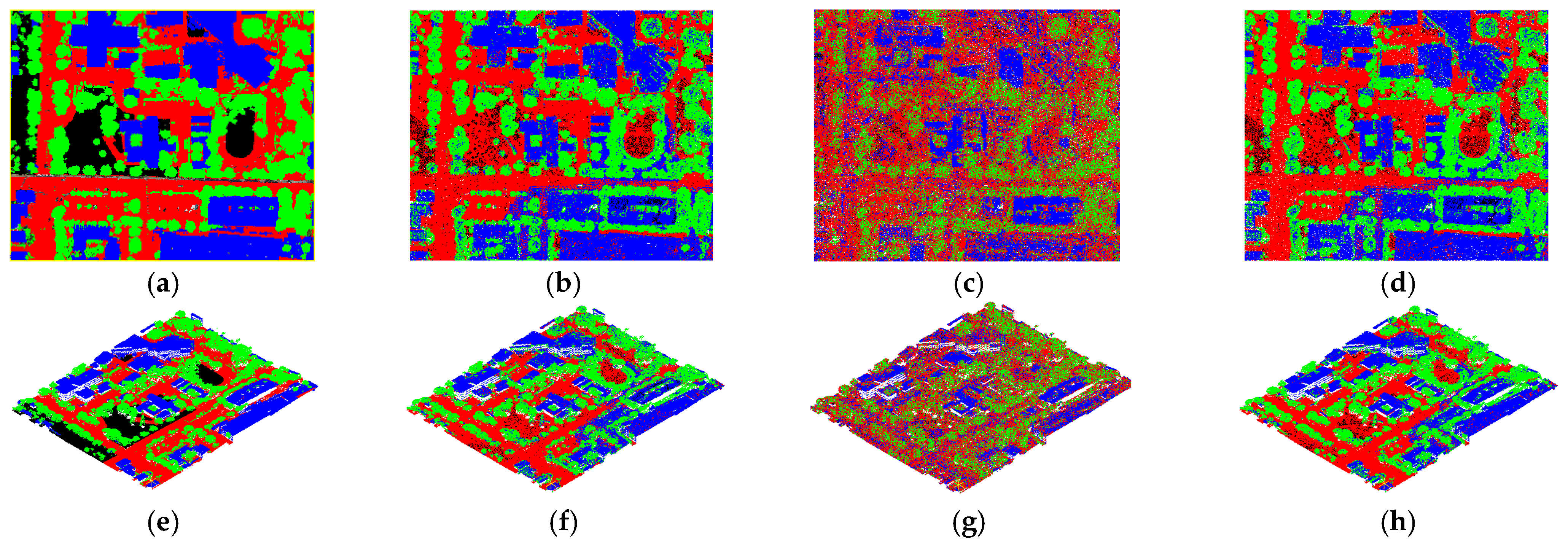
3.2. Comparisons between Different Data Sources

Two single-source feature subsets F_2 and F_3 represented the features from the airborne LiDAR point clouds and the features from the high-resolution optical images, respectively. Random Forest was chosen as the classifier, 10% of the data in the sample area was extracted as the training data, F_1, F_2 and F_3 were used for the training of the classifier, and the point clouds in the test area A3 were used as the test data set for object classification and evaluation, and the classification results and classification accuracy based on different data sources were statistically obtained, as well as the respective classification effect plots shown in Figure 3, where (a)~(d) are the top views of the point clouds, and (e)~(h) are the corresponding side views of the point clouds.

The classification results using a single data source were not as excellent as the classification results utilizing fused data sources, as shown by the classification results of each category of features and the total classification accuracy in

Table 2. Classification results of each type of objects with different feature subsets from different data sources.

	Precision				Recall				OA
Feature Sets	Is	Gr	Tr	Ho	Is	Gr	Tr	Ho
F_1	76.7%	76.3%	80.7%	70.7%	77.2%	10.3%	92.3%	87.0%	76.2%
F_2	76.2%	53.3%	80.6%	66.5%	76.0%	10.8%	88.1%	84.9%	74.2%
F_3	48.7%	24.3%	42.7%	49.6%	55.2%	3.6%	47.4%	50.1%	46.9%

. In terms of the accuracy and recall rates of the four feature categories, the classification results using the F_1 feature set were better than those using the F_2 feature set or the F_3 feature set, except for the low vegetation category for which the recall rate of the F_1 feature set was slightly lower than that of the F_2 feature set, including the overall accuracy index. Figure 3c,g shows that the vegetation index features and texture features in the F_3 feature set had a certain role in the classification extraction of the building class, and the contours of the extracted buildings were more obvious, but there was a serious pretzel phenomenon; among the classification results of the two single-source data, the classification results using the F_3 feature set from the image data source were the worst.

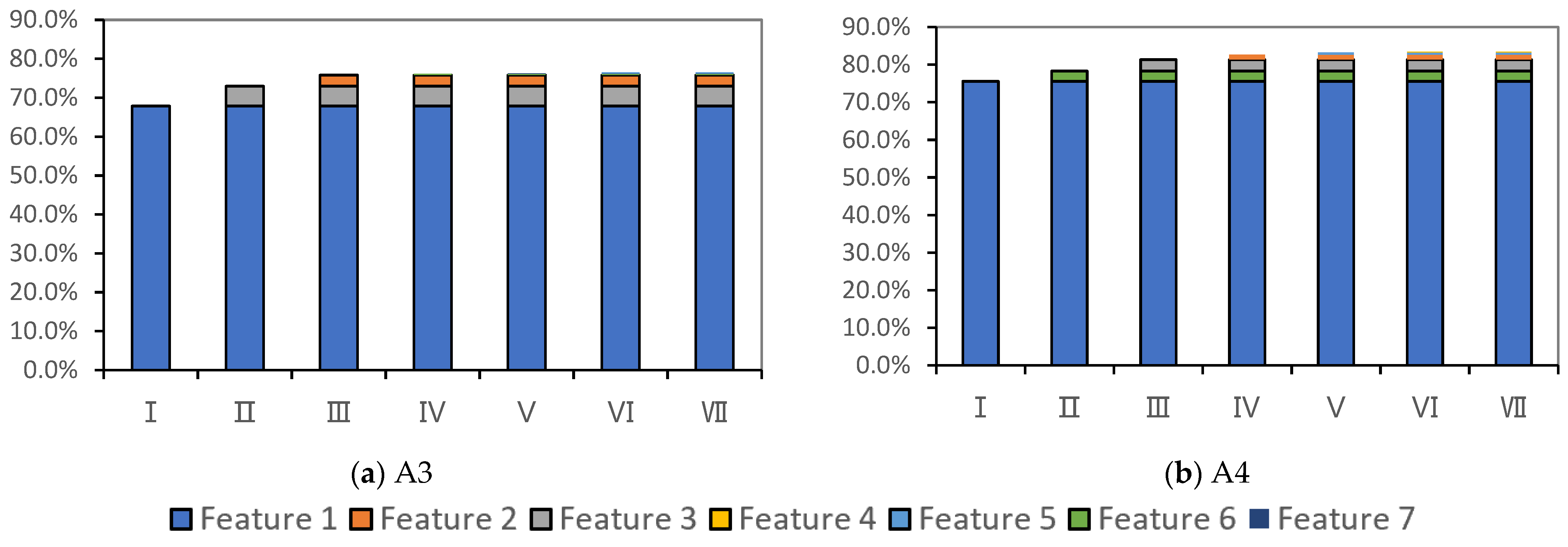
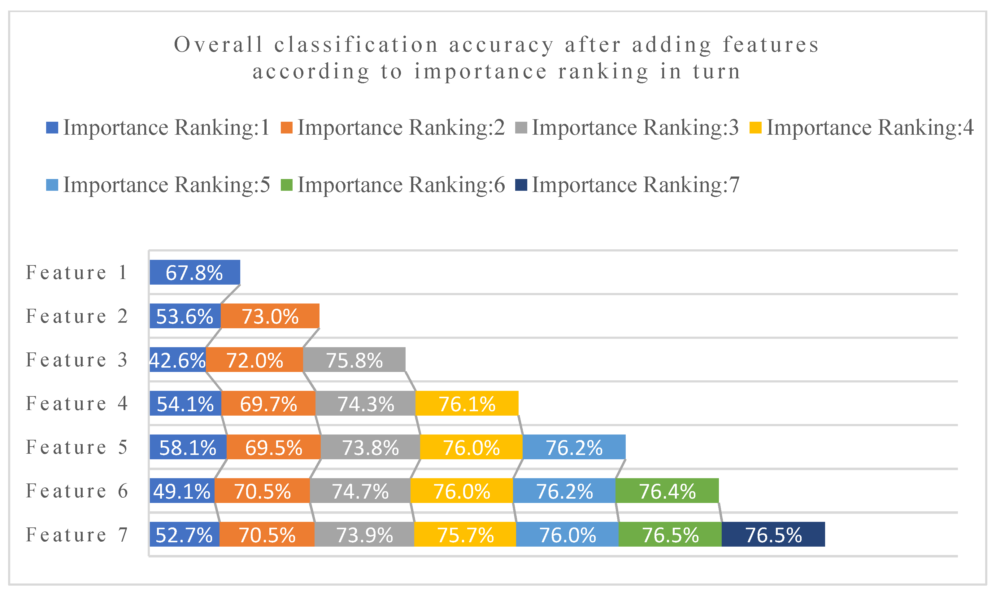
3.3. Combination and Optimization of Features

In the process of classifying a test region, the more feature dimensions in the feature set used is not the better. On the contrary, a reasonable selection of features and their dimensions can guarantee the classification accuracy to a certain extent and shorten the classifier’s training period.

The RF model is chosen as the classifier. By randomly selecting 10% of the data from the training area as training data and using 5-fold cross-validation, the RF model is obtained to classify the training area. The OA obtained by the PCA method is shown in Figure 4. Features one to seven are {$MAD\_1$,$MAD\_2$}, {$GLCM\_V$,$GLCM\_ASM$,$GLCM\_ENT$,$GLCM\_H$}, {$I_n$}, {$NGRDI$}, {$H_{skw}$,$H_{kur}$}, {$S_n$}, {$N_h$}, respectively.

According to Figure 4, the feature set F_4 of proper dimensionality obtained is {$MAD\_1$,$MAD\_$2,$GLCM\_V$,$GLCM\_ASM$,$GLCM\_ENT$,$GLCM\_H$,$I_n$,$NGRDI$}, which corresponds to an overall classification accuracy of 84.5%, which is only 0.5% lower than the highest overall classification accuracy, and effectively reduces the feature dimensionality. The sampling proportion is now set to 30%, and the feature sets F_4 are selected for test areas A3 and A4 respectively using the above sequential stepwise selection method, and their respective feature sets F_4 are obtained as {$MAD\_1$,$MAD\_2$,$I_n$,$GLCM\_V$,$GLCM\_ASM$,$GLCM\_ENT$,$GLCM\_H$} and {$MAD\_1$,$MAD\_2$,$S_n$,$I_n$,$GLCM\_V$,$GLCM\_ASM$,$GLCM\_ENT$,$GLCM\_H$}, respectively. After comparison, the overall classification accuracy of these two regions with feature set F_4 is 75.8% and 82.6%, respectively, which is only 0.67% and 0.81% lower than the overall classification accuracy obtained with the total feature set F_1 (Figure 5). The overall classification accuracy decreases slightly when the last feature is added to the feature subset c{$MAD\_1$,$MAD\_2$,$I_n$,$GLCM\_V$,$GLCM\_ASM$,$GLCM\_ENT$,$GLCM\_H$,$S_n$,$N_h$,$H_{skw}$,$H_{kur}$}, which shows that more dimensions of features in the feature set is not for the better. In addition, the increase in the overall classification accuracy after adding more features to the feature set F_4 is almost negligible, and the time to train the classifier increases accordingly. While using feature set F_5 as the training sample of the RF classifier, the overall classification accuracy obtained on the A3 test area is 74.0%, which is lower than the result of feature set F_4.

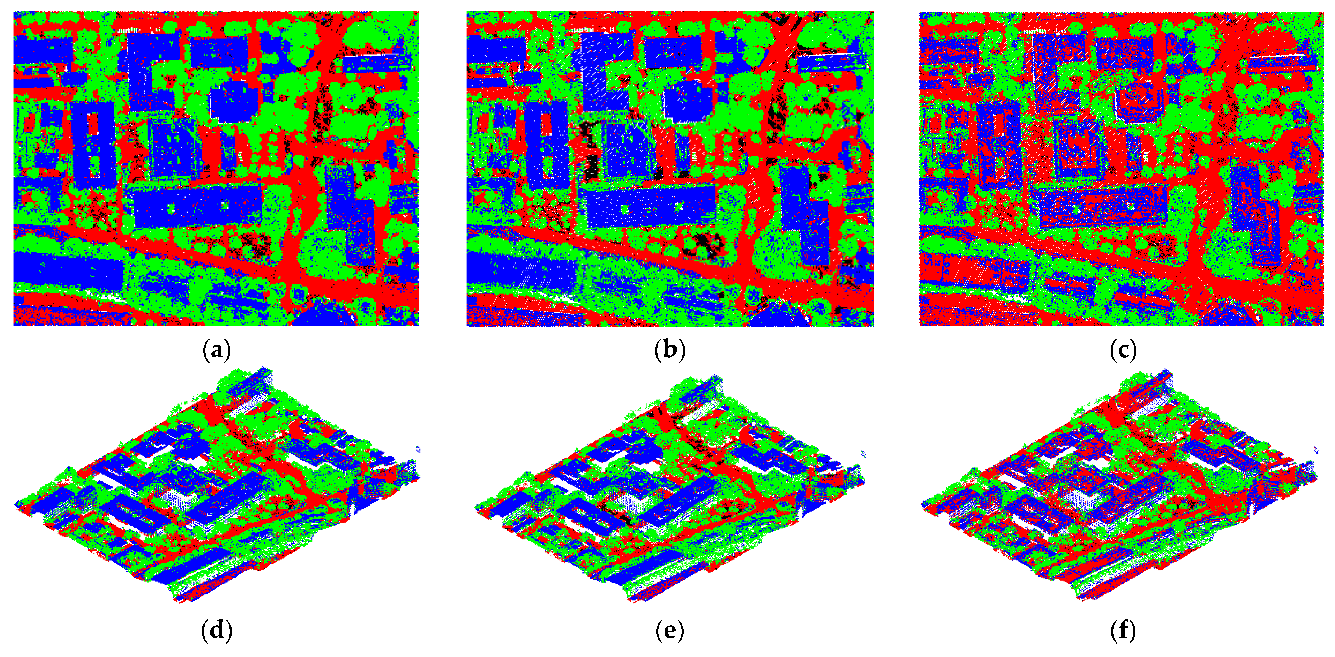
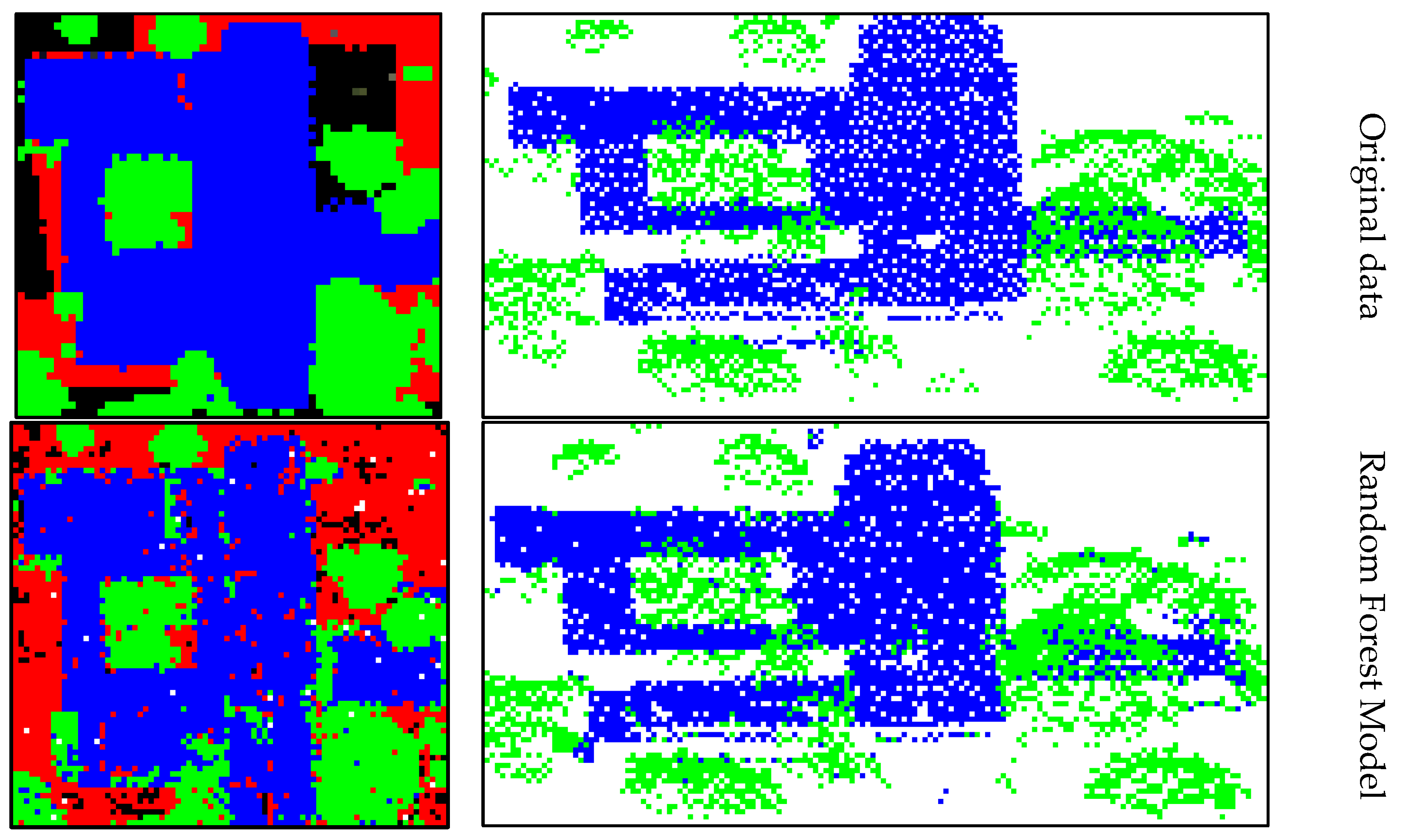
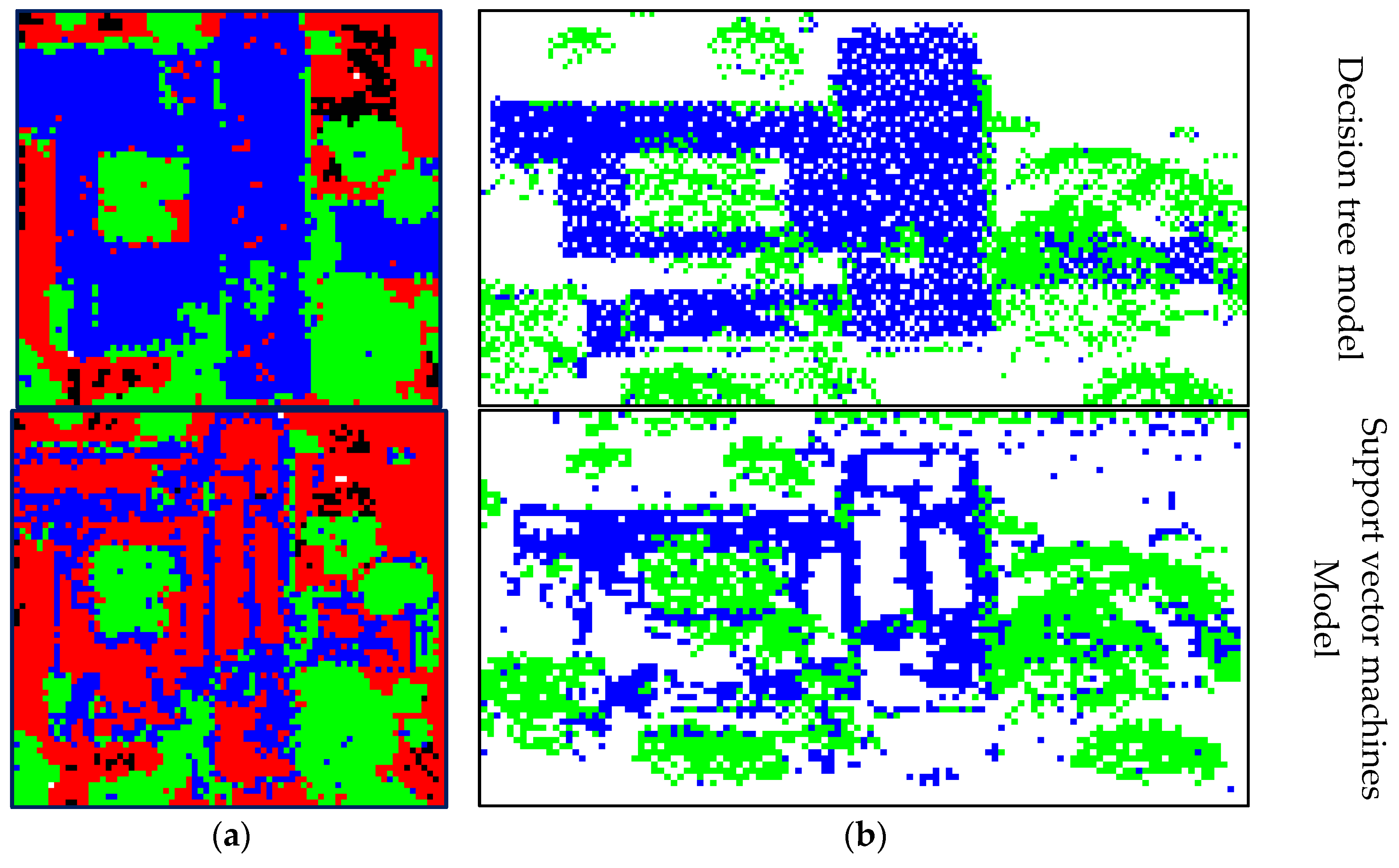
3.4. Effect of Different Classifiers on Classification Results

Under the same parameter conditions, the classification effect of different classifiers for the same test area may be very different. In this study, we used three different classifiers (RF,DT,SVM) to classify the point clouds in test areas A3 and A4, and obtain the precision and recall rates, and the overall classification accuracy of two types of features, namely trees and buildings, by counting the classification results, as shown in

Table 3. Accuracy table of the classification results of these three different models.

		Random Forest			Decision Tree			Support Vector Machine
		Precision	Recall	OA	Precision	Recall	OA	Precision	Recall	OA
A3	Tr	80.7%	92.3%	76.2%	76.0%	90.8%	74.5%	83.0%	87.9%	68.6%
	Ho	70.7%	87.0%		67.3%	83.8%		59.0%	62.0%
A4	Tr	82.9%	91.1%	83.3%	79.3%	90.1%	80.8%	85.6%	83.3%	74.6%
	Ho	79.7%	83.1%		76.8%	80.6%		72.0%	60.2%

, Figure 6 and Figure 7. The extraction rate of the sample data was 10%, and the classification feature set used is F_1.

Figure 6 and (a) to (c) in Figure 7 show the top views of the point clouds in different classifiers, and (d) to (f) show the corresponding side views.

According to the results in Table 3, for test areas A3 and A4, the overall classification accuracy obtained using the RF model was the highest, 76.2% and 83.3%, respectively; the DT was the second highest, 74.5% and 80.8%, respectively; and the SVM was the worst, 68.6% and 74.6%, respectively. Combining the results in Table 3, Figure 6 and Figure 7, the classification results of RF and DT are significantly better than the SVM model, and the RF classifier is more practical than the other two classifiers. The SVM, due to its own characteristics, not only has the phenomenon of overfitting, but also has a more serious pretzel phenomenon; the classification accuracy obtained using the sample data set (sampling proportion of 30%) as the test data are 76.4%, while the classification accuracy obtained using the test area A3 as the test data are 69.8%, as shown in Figure 6c,f and Figure 7c,f. The feature classification results of the SVM model are poorer than the other two classifiers, while the RF, as an integrated classifier with DT as the core, and in the experimental results of this study, is slightly better in terms of overall classification accuracy than the DT. It is worth noting that although the overall classification accuracy of the RF is the highest, the recall rates of both tree points and building points are lower than the results of the DT according to the accuracy analysis data in Table 3.

From Figure 6 and Figure 7, it can be seen that there are some rather special areas in the data species of this study: point clouds of other categories are included inside the building. In this study, we find a more typical special region S_1 and S_2 (red box in Figure 2) for each of the test areas A3 and A4. The results of the three classifiers are compared, and Figure 8 and Figure 9 are obtained: it is obvious that both the RF and DT classifiers have better classification results, and can effectively separate the tree points and impervious surface points from the building itself, while the SVM classifier has a significant and large number of misclassified points in this area.

4. Discussion

4.1. Sensitivity Analysis of the Proportion of Sample Sets

In the process of building classifiers using sample sets, a sample set with too small data volume may lead to overfitting; while a sample set with higher data volume will lead to higher classification accuracy, it will definitely take a longer time to build classifiers, especially for nonlinear classifiers, as the huge computation makes it difficult to build classifiers quickly. In this study, we used 5% as the step size, the sample set was extracted from 5% to 100%, and the extraction area was still the training area A1 and A2; then, we used the K-fold validation (K = 5) method to analyze the impact of different ratios on the classification results, and used the overall classification accuracy as the index to roughly estimate the appropriate extraction ratio range, and used it for the subsequent experiments to improve classification accuracy.

As can be seen from Figure 10, the sampling proportion in the process of constructing the sample set shows a positive correlation with the overall classification accuracy, and the sampling proportion at 30% can retain a certain amount of classification accuracy while achieving an overall classification accuracy of 86.4%, which is only 1% lower than the highest overall classification accuracy. Using A4 as the test dataset, the overall classification accuracy of the 30% sampling proportion in the actual classification was verified to be 84.1%, which was only 0.05% lower than the highest overall classification accuracy obtained by using 100% sampling proportion.

According to the above classification results, the feature set F_1 was used as the classification feature set to participate in the training, and the classifier was chosen as RF with a sample set extraction ratio of 30% to classify and count the overall point clouds; the final overall classification accuracy was 84.3%, among which the overall classification accuracy of the point clouds within the training area A2 was the highest at 91.5%; the overall classification accuracy of the training area A1 ranked second. The overall classification accuracy of the point clouds in the training area A2 was the highest, at 91.5%. Also, we can note that with the same classifier (RF) and sampling ratio (30%), the overall classification accuracy of the whole point cloud is 87.6% and the accuracy of the four objects is 88.5% (Is), 76.7% (Gr), 87.2% (Tr) and 88.3% (Ho) after training the classification model using the feature set F_4 obtained through the A4 region. It also shows that the selection of features is very necessary.

4.2. Differences Analysis between Selected Feature Sets

Different types of features have different roles and respective degrees of importance in the classification process of different regions, and there is a mutual suppression effect among features of the same type. The experimental results show that the five elevation-related features of $MAD\_1$,$MAD\_2$,$N_h$,$H_{skw}$,$H_{kur}$ have the relationship of mutual influence, and the $MAD\_1$,$MAD\_2$ features can suppress the improvement of the other three features in classification accuracy.

The $MAD\_1$,$MAD\_2$ features are classified based on the neighborhood statistics of normalized elevation, which can effectively classify features with a certain elevation such as buildings and trees. The features show the direction of the normal vector, which can effectively distinguish between flat and non-flat features, so the features contribute a more important role in distinguishing buildings and trees. Texture features can obtain texture information and help machine learning models to classify features with large textural differences.

Figure 5 and Figure 6 above show that in feature set F_1, the features that have the greatest influence on the classification results are $MAD\_1$,$MAD\_2$ features; for the classification results in different sources, the features with the second highest importance differ, for regions A1 and A2 corresponding to texture features, region A3 corresponding to intensity features In, and region A4 corresponding to normal vectors $S_n$. The four regions are selected step by step according to the order to get the feature set F_4 which all contain $MAD\_1$,$MAD\_2$,$GLCM\_V$,$GLCM\_ASM$,$GLCM\_ENT$,$GLCM\_H$,$I_n$ features.

In Figure 11, features 1 to 7 are, respectively, {$MAD\_1$,$MAD\_2$};$S_n$;{$GLCM\_V$,$GLCM\_ASM$,$GLCM\_ENT$,$GLCM\_H$};$I_n$;$N_h$;{$H_{skw}$,$H_{kur}$};$NGRDI$. As seen in Figure 11, in the first round of conducting the first feature selection, five features related to elevation show different degrees of importance, and features occupy the first and second importance rankings, respectively, and the overall classification accuracy obtained from other features is significantly different, and the overall classification accuracies obtained by using them as feature sets are 67.8% and 58.1%, respectively; these two types of features are related to elevation, and the $N_h$ features are normalized elevation values, while the feature {$MAD\_1$,$MAD\_2$} are based on the neighborhood elevation statistics. Moreover, according to the feature selection process in the later rounds, it can be found that the degree of improvement of the $N_h$ features on the overall classification accuracy is always inferior to that of $I_n$,$S_n$,{$GLCM\_V$,$GLCM\_ASM$,$GLCM\_ENT$,$GLCM\_H$} in the case that there are already {$MAD\_1$,$MAD\_2$} features in the feature set; in the other two features $H_{skw}$,$H_{kur}$ related to elevation, the improvement of the overall classification accuracy is even weaker. With the other features whose attributes do not come from the elevation and its statistics, adding them to the feature set can instead effectively improve the overall classification accuracy. For example, the feature with the lowest improvement in overall classification accuracy in the first round was selected in feature set F_4 because it ranked second in the second round and first in the third round. The same performance is also observed for feature $S_n$, which ranked fourth in the first round and first in the second round.

4.3. AdaBoost (Adaptive Boosting) Classifier and Sample Imbalance Problem

According to the results in Table 2, the recall of feature Gr is obviously too low because the sample size of the feature is too small and there is an imbalance problem between the feature and other samples, while the integrated classifier AdaBoost based on augmented learning can effectively solve the sample imbalance problem. The main idea of the AdaBoost classifier is to use a multi-round iterative approach, where each iteration of training will update the sample weights based on the previous classification. The main idea of the AdaBoost classifier is to use multiple iterations, where each iteration updates the weights of the samples based on the previous classification results and adds new basic classifiers until a predefined small enough error rate or a pre-specified maximum number of iterations is reached. In this paper, the DT classifier is used as the basic classifier, the number of iterations is set to 30, Bayes is used to optimize the training process of this classifier, and the final feature Gr recall obtained with the DT classifier with single-source and multi-source data as training data are shown in

Table 4. Recall of Feature Gr under different combination schemes.

Method	F_1			F_3
	Precision	Recall	OA	Precision	Recall	OA
DT	47.90%	8.50%	50.40%	81.70%	40.50%	83.30%
AdaBoost	48.30%	17.10%	52.50%	85.90%	40.10%	86.20%

. Moreover, the recall rate of Gr features obtained using fused data + AdaBoost is 40.1% under the condition that the sampling proportion parameter is 30%, which is much higher than the corresponding value of 17.1% obtained using optical image data + AdaBoost, thus demonstrating again that the use of data feature fusion can effectively improve the classification accuracy of small samples. On the other hand, under the condition of two data sources, the AdaBoost classifier can improve the recall rate of Gr features from the optical image source data by 8.6%, which is about double, indicating that the reinforcement learning of the AdaBoost classifier can also solve the sample size imbalance problem; however, in the fused data source, it decreases by 0.4% instead, thus showing that the use of feature fusion is more important than the use of a more advanced classifier.

4.4. Limitations of the Proposed Method

In this paper, optical image data of 2D structure types and point cloud data of 3D structure types are fused in the feature fusion stage, and then feature information is extracted from different dimensions to increase the accuracy of classification; however, some points that overlap in vertical direction have some shared features, which leads to some classification errors. Secondly, there are other problems in this study: the unbalanced sample size of different features is the main reason for misclassification of features with small sample size. Due to the complexity of urban features, the recall rate of features with a smaller percentage is not high. We have tried to train the classifier model using the same sample size, but the final accuracy obtained is not high. In addition, the small density of LiDAR point clouds caused some certain point clouds not to be classified correctly. Due to the small point cloud density of the airborne LiDAR in this paper, and the incomplete shape of residential buildings under lush tree canopies, and even the existence of point cloud regions where the boundaries of the buildings and the tree canopies are indistinguishable, some difficulties were encountered in the classification process of the classifier.

5. Conclusions

In this study, LiDAR point cloud data and high-resolution optical image data were used as research objects, and feature sets were constructed by analyzing their respective data characteristics and extracting their features, using single-source feature sets as well as multi-source feature sets to train three models of RF, DT, and SVM, respectively, using the trained models to classify the point cloud data for the common urban areas of trees, buildings, impervious surfaces. The four types of features, namely trees, buildings, impervious surfaces, and low vegetation, were classified using the trained models. The following conclusions were obtained during the experiments: under the conditions of using the same number of samples and the same model, the effect of machine learning classification based on multi-source data was better than that of single-source data; the experiments on feature selection showed that some features play a similar role in the classification process of point clouds; in addition, the classification results of different classifiers vary greatly: the best result was obtained by the random forest classifier, while the SVM classifier had the worst result. With the increase in sample size, the overall classification accuracy of the three classifiers also showed a positive correlation growth, and from the perspective of classification accuracy and time consumption, the random forest model was more suitable for point cloud data classification in this study.

In the representation of point cloud data, there are certain differences between urban feature types, especially between spatial distributions, while image data has rich texture information and spectral information that point cloud data does not have, and the fusion of the two features can effectively improve the classification accuracy. If more point cloud features are added that are specific to different feature types, or richer multispectral features are added, the accuracy of point cloud classification may be further improved, and finer feature extraction can be performed. With the development of technology, point cloud classification methods under the fusion of more multi-source data will be explored in future work.

References

1. Dayo, Z.A.; Cao, Q.; Wang, Y.; Pirbhulal, S.; Sodhro, A.H. A Compact High-Gain Coplanar Waveguide-Fed Antenna for Military RADAR Applications. Int. J. Antennas Propag. 2020, 2020, 8024101. [Google Scholar] [CrossRef]
2. Cheng, Z.; Ma, H. Automatic Extracting and Modeling Approach of City Cloverleaf from Airborne LiDAR Data. Acta Geod. Cartogr. Sin. 2012, 41, 7. [Google Scholar]
3. Sampath, A.; Shan, J. Segmentation and Reconstruction of Polyhedral Building Roofs from Aerial Lidar Point Clouds. IEEE Trans. Geosci. Remote Sens. 2010, 48, 1554–1567. [Google Scholar] [CrossRef]
4. Sohn, G.; Huang, X.; Tao, V. Using a Binary Space Partitioning Tree for Reconstructing Polyhedral Building Models from Airborne Lidar Data. Photogramm. Eng. Remote Sens. 2008, 74, 1425–1440. [Google Scholar] [CrossRef]
5. Zhang, L.; Li, Z.; Li, A.; Liu, F. Large-scale urban point cloud labeling and reconstruction. ISPRS J. Photogramm. Remote Sens. 2018, 138, 86–100. [Google Scholar] [CrossRef]
6. Tan, K.; Du, P. Hyperspectral remote sensing image classification based on support vector machine. J. Infrared Millim. Waves 2008, 27, 6. [Google Scholar] [CrossRef]
7. Peng, D.; Zhang, Y.; Xiong, X. 3D Building Change Detection by Combining LiDAR Point Clouds and Aerial Imagery. Geomat. Inf. Sci. Wuhan Univ. 2015, 40, 7. [Google Scholar] [CrossRef]
8. Mu, C.; Yu, J.; Xu, L.; Dun, P. Geomatics and Information Science of Wuhan University. Geomat. Inf. Sci. Wuhan Univ. 2009, 34, 414–417. [Google Scholar]
9. Rebecca, L.P.; Dar, A.R.; Philip, E.D.; Laura, L.H. Sub-pixel mapping of urban land cover using multiple endmember spectral mixture analysis: Manaus, Brazil. Remote Sens. Environ. 2007, 106, 253–267. [Google Scholar] [CrossRef]
10. Paolo, G.; Fabio, D.A.; Belur, V.D. Urban remote sensing using multiple data sets: Past, present, and future. Inf. Fusion 2005, 6, 319–326. [Google Scholar] [CrossRef]
11. Song, J.H.; Han, S.H.; Yu, K.; Kim, Y.I. Assessing the possibility of land-cover classification using lidar intensity data. Int. Arch. Photogramm. Remote Sens. Spat. Inf. Sci. 2012, 34, 259–262. [Google Scholar]
12. Bellakaout, A.; Cherkaoui, M.; Ettarid, M.; Touzani, A. Automatic 3D Extraction of Buildings, Vegetation and Roads from LIDAR Data. ISPRS Int. Arch. Photogramm. Remote Sens. Spat. Inf. Sci. 2016, 41, 173–180. [Google Scholar] [CrossRef]
13. Zhang, J.; Lin, X.; Ning, X. SVM-Based Classification of Segmented Airborne LiDAR Point Clouds in Urban Areas. Remote Sens. 2013, 5, 3749–3775. [Google Scholar] [CrossRef] [Green Version]
14. Zhou, M.; Kang, Z.; Wang, Z.; Kong, M. Airborne lidar point cloud classification fusion with dim point cloud. ISPRS Int. Arch. Photogramm. Remote Sens. Spat. Inf. Sci. 2020, 43, 375–382. [Google Scholar] [CrossRef]
15. Guo, L.; Chehata, N.; Mallet, C.; Boukir, S. Relevance of airborne lidar and multispectral image data for urban scene classification using Random Forests. ISPRS J. Photogramm. Remote Sens. 2011, 66, 56–66. [Google Scholar] [CrossRef]
16. Su, W.; Li, J.; Cheng, Y.; Zhang, J.; Hu, D.; Liu, C. Object-oriented Urban Land-cover Classification of Multi-scale Image Segmentation Method—A Case Study in Kuala Lumpur City Center, Malaysia. Natl. Remote Sens. Bull. 2007, 11, 521–530. [Google Scholar] [CrossRef]
17. Cheng, X.; Cheng, X.; Hu, M.; Guo, W.; Zhang, L. Buildings Detection and Contour Extraction by Fusion of Aerial Images and LIDAR Point Cloud. Chin. J. Lasers 2016, 43, 9. [Google Scholar] [CrossRef]
18. Suarez, J.; Ontiveros, C.; Smith, S.; Snape, S. Use of airborne LiDAR and aerial photography in the estimation of individual tree heights in forestry. Comput. Geosci. 2005, 31, 253–262. [Google Scholar] [CrossRef]
19. Wang, X.; Li, P. Extraction of urban building damage using spectral, height and corner information from VHR satellite images and airborne LiDAR data. ISPRS J. Photogramm. Remote Sens. 2020, 159, 322–336. [Google Scholar] [CrossRef]
20. Awrangjeb, M.; Zhang, C.; Fraser, C.S. Automatic extraction of building roofs using LIDAR data and multispectral imagery. ISPRS J. Photogramm. Remote Sens. 2013, 83, 1–18. [Google Scholar] [CrossRef]
21. Parsian, S. Combining Hyperspectral and LiDAR Data for Building Extraction using Machine Learning Technique. Int. J. Comput. 2017, 2, 88–93. [Google Scholar]
22. Qixia, M.; Pinliang, D.; Huadong, G. Pixel- and feature-level fusion of hyperspectral and lidar data for urban land-use classification. Int. J. Remote Sens. 2015, 36, 1618–1644. [Google Scholar] [CrossRef]
23. Uezato, T.; Fauvel, M.; Dobigeon, N. Lidar-Driven Spatial Regularization for Hyperspectral Unmixing. In Proceedings of the IGARSS 2018—2018 IEEE International Geoscience and Remote Sensing Symposium, Valencia, Spain, 22–27 July 2018; pp. 1740–1743. [Google Scholar]
24. Wang, Y.; Chen, Q.; Liu, L.; Li, X.; Sangaiah, A.K.; Li, K. Systematic Comparison of Power Line Classification Methods from ALS and MLS Point Cloud Data. Remote Sens. 2018, 10, 1222. [Google Scholar] [CrossRef]
25. Jingjing, C.; Kai, L.; Li, Z.; Lin, L.; Yuanhui, Z.; Liheng, P. Combining UAV-based hyperspectral and LiDAR data for mangrove species classification using the rotation forest algorithm. Int. J. Appl. Earth Obs. Geoinf. 2021, 102, 102414. [Google Scholar] [CrossRef]
26. Xiong, Y.; Gao, R.; Xu, Z. Random Forest Method for Dimension Reduction and Point Cloud Classification Based on Airborne LiDAR. Acta Geod. Cartogr. Sin. 2018, 47, 11. [Google Scholar] [CrossRef]
27. Mallet, C.; Bretar, F.; Roux, M.; Soergel, U.; Heipke, C. Relevance assessment of full-waveform lidar data for urban area classification. ISPRS J. Photogramm. Remote Sens. 2011, 66, S71–S84. [Google Scholar] [CrossRef]
28. Zhang, Z.; Zhang, L.; Tong, X.; Bo, G.; Liang, Z.; Xing, X. Discriminative-Dictionary-Learning-Based Multilevel Point-Cluster Features for ALS Point-Cloud Classification. IEEE Trans. Geosci. Remote Sens. 2016, 54, 7309–7322. [Google Scholar] [CrossRef]
29. Liu, Y.; Liu, Y.; Hu, X.; Xiu, L. Airborne LiDAR Point Cloud Classification in Urban Area Based on XGBoost and CRF. Remote Sens. Inf. 2020, 35, 5. [Google Scholar] [CrossRef]
30. Dalponte, M.; Bruzzone, L.; Gianelle, D. Fusion of Hyperspectral and LIDAR Remote Sensing Data for Classification of Complex Forest Areas. IEEE Trans. Geosci. Remote Sens. 2008, 46, 1416–1427. [Google Scholar] [CrossRef]
31. Du, N.; Peng, J. Decision-tree-based classification of airborne LiDAR point clouds. Sci. Surv. Mapp. 2013, 38, 118–120. [Google Scholar]
32. Xu, F.; Zhang, X.; Shi, Y. Research on Classification of Land Cover based on LiDAR Cloud and Aerial Images. Remote Sens. Technol. Appl. 2019, 34, 10. [Google Scholar] [CrossRef]
33. Dong, B. Research on Feature Classification Technology by Fusion of Airborne LiDAR Point Cloud and Remote Sensing Images; Information Engineering University: Zhengzhou, China, 2013. [Google Scholar]
34. Mahmoudabadi, H.; Shoaf, T.; Olsen, M. Superpixel Clustering and Planar Fit Segmentation of 3D LIDAR Point Clouds. In Proceedings of the 2013 Fourth International Conference on Computing for Geospatial Research and Application, San Jose, CA, USA, 22–24 July 2013; pp. 1–7. [Google Scholar] [CrossRef]
35. Hu, H.; Hui, Z.; Hui, Z. Airborne LiDAR Point Cloud Classification Based on Multiple-Entity Eigenvector Fusion. Chin. J. Lasers 2020, 47, 11. [Google Scholar]
36. Ghamisi, P.; Benediktsson, J. Feature Selection Based on Hybridization of Genetic Algorithm and Particle Swarm Optimization. IEEE Geosci. Remote Sens. Lett. 2015, 12, 309–313. [Google Scholar] [CrossRef]
37. Rasti, B.; Ghamisi, P.; Plaza, J.; Plaza, A. Fusion of Hyperspectral and LiDAR Data Using Sparse and Low-Rank Component Analysis. IEEE Trans. Geosci. Remote Sens. 2017, 55, 6354–6365. [Google Scholar] [CrossRef]
38. Chehata, N.; Guo, L.; Mallet, C. Airborne LIDAR feature selection for urban classification using random forests. ISPRS Int. Arch. Photogramm. Remote Sens. Spat. Inf. Sci. 2009, 38, 207–212. [Google Scholar]
39. Zhang, W.; Qi, J.; Wan, P.; Wang, H.; Yan, G. An Easy-to-Use Airborne LiDAR Data Filtering Method Based on Cloth Simulation. Remote Sens. 2016, 8, 501. [Google Scholar] [CrossRef]
40. Bentley, J.L. Multidimensional binary search trees used for associative searching. Commun. ACM 1975, 18, 509–517. [Google Scholar] [CrossRef]
41. Zhang, K.; Qiao, S.; Kai, G. A new point cloud reconstruction algorithm based-on geometrical features. In Proceedings of the International Conference on Modelling, Identification and Control, Sousse, Tunisia, 18–20 December 2015. [Google Scholar]
42. Breiman, L.; Breiman, L.; Cutler, R.A. Random Forests Machine Learning. J. Clin. Microbiol. 2001, 2, 199–228. [Google Scholar]
Figure 1. Flowchart of research method.
Electronics 11 03041 g001
Figure 2. Experimental data sources: (a) optical image; (b) top view of ALS LiDAR point cloud.
Electronics 11 03041 g002
Figure 3. Point cloud classification results from different data sources: (a) original data in top view; (b) result from optical image in top view; (c) result from LiDAR in top view; (d) result from data fusion in top view; (e) original data in side view; (f) result from optical image in side view; (g) result from LiDAR in side view; (h) result from data fusion in side view.
Electronics 11 03041 g003
Figure 4. Overall classification accuracy after adding features according to PCA ranking.
Electronics 11 03041 g004
Figure 5. Overall classification accuracy after adding features according to PCA ranking for test area A3, A4.
Electronics 11 03041 g005
Figure 6. Classification effect of different models in training area A3: (a,d) are the classification results of the RF model from a top and side view, respectively; (b,e) are the classification results of the DT model from a top and side view, respectively; (c,f) are the classification results of the SVM model from a top and side view, respectively.
Electronics 11 03041 g006
Figure 7. Classification results of different models in training area A4: (a,d) are the classification results of the RF model from a top and side view, respectively; (b,e) are the classification results of the DT model from a top and side view, respectively; (c,f) are the classification results of the SVM model from a top and side view, respectively.
Electronics 11 03041 g007
Figure 8. Point cloud classification results of experimental area S_1. (a) Top view. (b) Side view (buildings and trees).
Electronics 11 03041 g008aElectronics 11 03041 g008b
Figure 9. Point cloud classification results of experimental area S_2. (a) Top view. (b) Side view (buildings and trees).
Electronics 11 03041 g009
Figure 10. The relationship between sampling rate and overall classification accuracy.
Electronics 11 03041 g010
Figure 11. Detailed data for each round of feature selection in the A3 region.
Electronics 11 03041 g011