Accurate Frequency Estimator for Real Sinusoid Based on DFT

Abstract

An accurate frequency estimator for real sinusoid based on Discrete Fourier Transform (DFT) is proposed. The proposed estimator is based on the interpolation of the maximum DFT spectral line and two Discrete-Time Fourier Transform (DTFT) spectral lines and can operate with both the rectangular window and the maximum sidelobe decay (MSD) window. In the coarse estimation step, the proposed estimator with the MSD window is used. According to the value of the coarse estimate, the negative frequency spectral component is removed. In the fine estimation step, the proposed estimator with the rectangular window is utilized to achieve the Cramer–Rao lower bound (CRLB). Simulation results show that the performance of this algorithm is better than that of the AM algorithm, Candan algorithm, Djukanovic algorithm, and FDIAM algorithm.

1. Introduction

Frequency estimation of sinusoidal signal in white noise is a classic topic in the field of digital signal processing. It can be widely used in numerous fields—for instance, in communications, radar signal processing, sonar, electronic measurement, etc. [1,2,3,4,5]. For example, Orthogonal Frequency Division Multiplexing (OFDM) technology is often used to realize multi-carrier transmission schemes. As we know, OFDM technology is very sensitive to frequency offsets, which will destroy the orthogonality between the subcarriers. Thus, it is necessary to accurately estimate the value of the frequency offset.

The existing frequency estimators can mainly be divided into two categories: time domain algorithms and frequency domain algorithms. Time domain algorithms include the maximum likelihood (ML) algorithms [6,7], the autocorrelation algorithms [8,9], the linear prediction algorithms [10], and the least square algorithms [11]. Nevertheless, due to the large amount of computation required, these algorithms are difficult to use in real-time applications. Frequency domain algorithms are usually implemented based on DFT [12,13,14,15,16,17,18,19,20]. These algorithms usually have small computational requirements. Therefore, they are suitable for real-time applications. Frequency estimators implemented based on DFT generally have two steps: coarse search and fine search. The coarse search is used to determine the maximum amplitude of DFT samples by a simple maximum search procedure. The fine search obtains the relative frequency deviation between the signal frequency and the coarse estimate by means of certain interpolation methods. The difference between different interpolation algorithms lies only in the second step. The Aboutanios and Mulgrew (AM) algorithm uses two spectral lines located halfway between the maximum spectral line and its two neighbors for the fine search [17]. Candan achieves the fine search by using the maximum spectral line and two spectral lines on the left and right of the maximum one [18]. Fang et al. firstly perform N-point time-domain zero-padding on the N-point sinusoidal sampling sequence, then use the amplitudes of the two spectral lines adjacent to the largest one in the 2N-point DFT spectrum to estimate the relative frequency deviation [19]. The recent progress of the fast algorithms based on DFT is discussed in [20], which utilizes prior knowledge of signal spectrum sparsity and signal detection index to reduce the computational complexity and improve the estimation performance. Candan obtains the fine frequency estimation by multiplying the sinusoid with arbitrary window functions and performing the interpolation of three spectral lines [21].

The signal model of all the above estimators is complex sinusoid. The real sinusoidal signal model is also often used in practical applications, and the frequency estimation of the real sinusoid is more complicated than that of complex sinusoid due to the problem of spectrum leakage from the negative frequency spectrum component of the signal. Many researchers have presented their algorithms for real sinusoid [22,23,24,25,26,27,28,29]. In [22], a frequency estimation algorithm similar to ML based on the spectrum matching method is proposed. The algorithm avoids the spectrum leakage problem by incorporating it into the signal or spectrum model. However, this algorithm requires an exhaustive search, which needs large amount of computation. In [23], the frequency of a real-valued tone can be estimated by extracting the instantaneous frequency based on the maximum distribution energy of the signal calculated from the time–frequency distribution (TFD). In [24], Djukanovic derives an algorithm based on the Candan algorithm [21] and AM algorithm [17], and the negative frequency spectrum component is shifted via modulation before the fine frequency estimation. When the signal-to-noise ratio (SNR) is sufficiently high or the frequency is small, the performance of the algorithm degrades [28]. In [28], a frequency domain iterative algorithm based on the AM (FDIAM) algorithm is proposed, which can realize the frequency estimation of real sinusoids without windows. In [29], a frequency estimator of real sinusoid combined with the algorithm in [12] is proposed, which has a high accuracy.

In this paper, an accurate frequency estimator of real sinusoid based on DFT is proposed. The proposed estimator is based on the interpolation of the maximum DFT spectral line and two DTFT spectral lines and can operate with both the rectangular window and the MSD window. In the coarse estimation step, the proposed estimator with the MSD window is used. According to the value of the coarse estimate, the negative frequency spectral component is removed. In the fine estimation step, the proposed estimator with the rectangular window is utilized to achieve the CRLB. Computer simulation results indicate that the performance of this algorithm is better than that of the AM algorithm [17], Candan algorithm [21], Djukanovic algorithm [24], and FDIAM algorithm [28].

The rest of this paper is arranged as follows. In the second section, we propose the new algorithm. In the third section, the performance of this algorithm is compared with that of other algorithms and the CRLB. Conclusions are given in the last section.

2. Proposed Estimation Algorithm

The model of single tone real sinusoid in additive white Gaussian noise is

$$x\left(n\right)=s\left(n\right)+z\left(n\right)n=0,1,\dots ,N-1$$

(1)

$$s\left(n\right)=A\cos \left(2\pi f_{0}n+\varphi \right)n=0,1,\dots ,N-1$$

(2)

where $N$ is the number of samples. $A$, $f_0$, and $\varphi$ are the amplitude, frequency, and initial phase of the sinusoid, respectively. The noise term $z(n)$ is assumed to be zero-mean additive white Gaussian noise with variance ${\sigma }_z^2$. Then, the SNR is $SNR=\frac{A^2}{2{\sigma }_z^2}$. The signal frequency can be expressed as

$$f_0=\left(k_m+\delta \right)/N$$

(3)

where $k_m$ is the discrete frequency index value of the maximum DFT spectral line and $\delta$ denotes the normalized fractional frequency offset, $\delta \in \left(-0.5,0.5\right)$.

The CRLB of frequency estimation for real sinusoid is [24]

$$\mathrm{var}\left({\widehat{f}}_0\right)\ge \frac{3}{{\pi }^{2}SNR·N\left(N^2-1\right)}$$

(4)

We know that the spectrum of a real sinusoid consists of positive and negative frequency spectrum components. According to Euler formula, the real sinusoid in Equation (2) can be expanded into

$$s\left(n\right)=A{e}^{j\phi }{e}^{j2\pi f_{0}n}/2+A{e}^{-j\phi }{e}^{-j2\pi f_{0}n}/2n=0,1,\dots ,N-1$$

(5)

The positive frequency part can be expressed as

$$s_{+}\left(n\right)=A{e}^{j\phi }{e}^{j2\pi f_{0}n}/2$$

(6)

and the negative frequency part is

$$s_{-}\left(n\right)=A{e}^{-j\phi }{e}^{-j2\pi f_{0}n}/2$$

(7)

The proposed estimation algorithm is implemented in three parts. In Section 2.1, a frequency estimation algorithm based on DFT and rectangular window is proposed. In Section 2.2, the estimator proposed in Section 2.1 is generalized to the case of MSD windows. In Section 2.3, a frequency estimation algorithm for real sinusoid implemented based on the estimators in Section 2.1 and Section 2.2 is proposed.

2.1. Proposed Frequency Estimator Based on Rectangular Window

Firstly, the N-point DFT of $s\left(n\right)$ is recorded as $S\left(k\right)$. In view of the symmetry of the DFT spectrum of a real sinusoid sequence, the negative frequency spectrum component is ignored. Then, we can obtain

$$S\left(k\right)=\frac{1}{2}{\displaystyle \sum _{n=0}^{N-1}A{e}^{j\phi }{e}^{j2\pi f_{0}n}{e}^{-j\frac{2\pi }{N}nk}}k=0,1,\dots ,N/2-1$$

(8)

For convenience, the N-point DFT coefficient is expressed as

$$S_l=\frac{1}{2}{\displaystyle \sum _{n=0}^{N-1}A{e}^{j\phi }{e}^{j2\pi f_{0}n}{e}^{-j2\pi \left(k_m+l\right)n/N}}$$

(9)

where $l$ represents the discrete frequency interval from $k_m$.

Then, Equation (3) is substituted into Equation (9), and we have

$$S_l=\frac{A{e}^{j\phi }}{2N}\frac{1-e^{j2\pi \left(\delta -l\right)}}{1-e^{j2\pi \left(\delta -l\right)/N}}$$

(10)

When $2\pi \left(\delta -l\right)\ll N$, the following formula can be obtained

$$e^{j2\pi \left(\delta -l\right)/N}\approx 1+j\frac{2\pi }{N}\left(\delta -l\right)$$

(11)

Then, we substitute Equation (11) into Equation (10), obtaining

$$S_l=\frac{b_l}{\delta -l}$$

(12)

in which

$$b_l=\frac{jA{e}^{j\phi }}{4\pi }\left[1-e^{j2\pi \left(\delta -l\right)}\right]$$

(13)

Then, $b_0$, $b_{0.1}$, and $b_{-0.1}$ are calculated according to Equation (13), and we have

$$b_0=\frac{jA{e}^{j\phi }}{4\pi }\left[1-e^{j2\pi \delta }\right]$$

(14)

$$b_{0.1}=\frac{jA{e}^{j\phi }}{4\pi }\left[1-U{e}^{j2\pi \delta }\right]$$

(15)

$$b_{-0.1}=\frac{jA{e}^{j\phi }}{4\pi }\left[1-Y{e}^{j2\pi \delta }\right]$$

(16)

in which

$$U=\cos \left(0.2\pi \right)-j\sin \left(0.2\pi \right)$$

(17)

$$Y=\cos \left(0.2\pi \right)+j\sin \left(0.2\pi \right)$$

(18)

Then, $S_0$, $S_{0.1}$, and $S_{-0.1}$ can be expressed as

$$S_0=\frac{jA{e}^{j\phi }}{4\pi }\frac{1-e^{j2\pi \delta }}{\delta }$$

(19)

$$S_{0.1}=\frac{jA{e}^{j\phi }}{4\pi }\frac{1-U{e}^{j2\pi \delta }}{\delta -0.1}$$

(20)

$$S_{-0.1}=\frac{jA{e}^{j\phi }}{4\pi }\frac{1-Y{e}^{j2\pi \delta }}{\delta +0.1}$$

(21)

Then, we have

$$\frac{S_{0.1}}{S_0}=\frac{1-U{e}^{j2\pi \delta }}{1-e^{j2\pi \delta }}\frac{\delta }{\delta -0.1}$$

(22)

$$\frac{S_{-0.1}}{S_0}=\frac{1-Y{e}^{j2\pi \delta }}{1-e^{j2\pi \delta }}\frac{\delta }{\delta +0.1}$$

(23)

After some algebra, we obtain

$$\frac{\left[S_{0.1}-U{S}_0\right]\delta -\left(0.1\right)S_{0.1}}{\left[S_{-0.1}-Y{S}_0\right]\delta +\left(0.1\right)S_{-0.1}}=\frac{1-U}{1-Y}$$

(24)

The estimation expression of $\delta$ can be obtained as

$$\widehat{\delta }=\mathrm{Re}\left\{\frac{\left(0.1\right)\left(1-Y\right)S_{0.1}+\left(0.1\right)\left(1-U\right)S_{-0.1}}{\left(1-Y\right)S_{0.1}-\left(1-U\right)S_{-0.1}+2j{S}_0\sin \left(0.2\pi \right)}\right\}$$

(25)

2.2. Proposed Frequency Estimator Based on MSD Window

The frequency estimation of real sinusoid is more complicated than that of a complex sinusoid because of the superposition of the positive and negative frequency spectrum components of real sinusoid. Multiplying a real sinusoid with a proper window function is an effective way to eliminate or reduce the estimation deviation. MSD windows have been widely used in references [13,14,15]. The sidelobe decay rate of H-term MSD window is equal to $6\left(2H-1\right)$ dB/octave, which is the highest among all the H-term cosine windows. In this part, an algorithm based on the estimator described in Section 2.1 and the MSD window is proposed. The expression of the H-term MSD window is [15]

$$w\left(n\right)={\displaystyle \sum _{h=0}^{H-1}{\left(-1\right)}^h{a}_h\cos \left(2\pi \frac{h}{N}n\right)}n=0,1,\dots ,N-1$$

(26)

where $a_h$ is the window coefficient and $H$ is the number of $a_h$ coefficients, $H\ge 1$. The expression of $a_h$ is

$$a_0=\frac{C_{2H-2}^{H-1}}{2^{2H-2}},a_h=\frac{C_{2H-2}^{H-h-1}}{2^{2H-3}}h=1,\dots ,N-1$$

(27)

The real sinusoid is multiplied by the MSD window, and we obtain

$$x_w\left(n\right)=x\left(n\right)·w\left(n\right)n=0,1,\dots ,N-1$$

(28)

Then, we perform DTFT on $x_w\left(n\right)$, and have

$$X_w\left(\lambda \right)=AW\left(\lambda -\delta \right)e^{j\phi }$$

(29)

If sufficiently large number of samples are obtained $\left(N\gg 1\right)$, then we have

$$\begin{gathered} W\left(\lambda \right)=\frac{N\sin \left(\pi \lambda \right)}{\pi }{\displaystyle \sum _{h=0}^{H-1}{\left(-1\right)}^h}{a}_h\frac{\lambda }{{\lambda }^2-h^2}{e}^{-j\pi \lambda } \\ =\tilde{W}\left(\lambda \right)e^{-j\pi \lambda }n=0,1,\dots ,N-1 \end{gathered}$$

(30)

in which

$$\tilde{W}\left(\lambda \right)=\frac{N\sin \left(\pi \lambda \right)}{\pi }{\displaystyle \sum _{h=0}^{H-1}{\left(-1\right)}^h}{a}_h\frac{\lambda }{{\lambda }^2-h^2},\left|\lambda \right|<2$$

(31)

From Equation (31), we can obtain

$${\tilde{W}}^{\prime }\left(\lambda \right)=\frac{N}{\pi }\left[\sin \left(\pi \lambda \right)+\pi \lambda \cos \left(\pi \lambda \right)\right]{\displaystyle \sum _{h=0}^{H-1}\frac{{{\left(-1\right)}^{h}a}_h}{{\lambda }^2-h^2}}-\frac{2N}{\pi }{\lambda }^2\sin \left(\pi \lambda \right){\displaystyle \sum _{h=0}^{H-1}\frac{{\left(-1\right)}^h{a}_h}{{\left({\lambda }^2-h^2\right)}^2}}$$

(32)

In Section 2.1, the estimation formula for the normalized frequency offset is expressed as Equation (25). We denote the part in the braces of Equation (25) as P and replace its corresponding spectral lines with $X_w\left(0\right)$, $X_w\left(0.1\right)$, and $X_w\left(-0.1\right)$. Then, we have

$$P=\frac{\left(0.1\right)\left(1-Y\right)X_w\left(0.1\right)+\left(0.1\right)\left(1-U\right)X_w\left(-0.1\right)}{\left(1-Y\right)X_w\left(0.1\right)-\left(1-U\right)X_w\left(-0.1\right)+2j{X}_w\left(0\right)\sin \left(0.2\pi \right)}$$

(33)

According to Equations (29) and (30), when $\lambda =0$, $0.1$, and $-0.1$, we have

$$X_w\left(0\right)=A\tilde{W}\left(-\delta \right)e^{j\phi }$$

(34)

$$X_w\left(0.1\right)=A\tilde{W}\left(0.1-\delta \right)e^{j\phi }{e}^{-j\left(0.1\pi \right)}$$

(35)

$$X_w\left(-0.1\right)=A\tilde{W}\left(-0.1-\delta \right)e^{j\phi }{e}^{j\left(0.1\pi \right)}$$

(36)

Substituting Equations (34)–(36) into Equation (33), we have

$$P=\frac{(0.1)(1-Y)\tilde{W}\left(0.1-\delta \right)e^{-j\left(0.1\pi \right)}+(0.1)(1-U)\tilde{W}\left(-0.1-\delta \right)e^{j\left(0.1\pi \right)}}{(1-Y)\tilde{W}\left(0.1-\delta \right)e^{-j\left(0.1\pi \right)}-(1-U)\tilde{W}\left(-0.1-\delta \right)e^{j\left(0.1\pi \right)}+2j\tilde{W}\left(-\delta \right)\sin (0.2\pi )}$$

(37)

Carrying out the first-order Taylor series expansion for $\tilde{W}\left(0.1-\delta \right)$, $\tilde{W}\left(-0.1-\delta \right)$, and $\tilde{W}\left(-\delta \right)$ near 0.1, −0.1, and 0, respectively, and ignoring the higher order terms, we have

$$\tilde{W}\left(0.1-\delta \right)\approx \tilde{W}\left(0.1\right)-{\tilde{W}}^{\prime }\left(0.1\right)\delta$$

(38)

$$\begin{gathered} \tilde{W}\left(-0.1-\delta \right)\approx \tilde{W}\left(-0.1\right)-{\tilde{W}}^{\prime }\left(-0.1\right)\delta \\ =\tilde{W}\left(0.1\right)+{\tilde{W}}^{\prime }\left(0.1\right)\delta \end{gathered}$$

(39)

$$\tilde{W}\left(-\delta \right)\approx \tilde{W}\left(0\right)-{\tilde{W}}^{\prime }\left(0\right)\delta$$

(40)

In Equation (39), we use the conclusion that $\tilde{W}\left(\lambda \right)$ is an even function and ${\tilde{W}}^{\prime }\left(\lambda \right)$ is an odd function [13].

Substituting Equations (38)–(40) into Equation (37), we have

$$P=\frac{\left(0.1\right)\left(1-Y\right)\left[\tilde{W}\left(0.1\right)-{\tilde{W}}^{\prime }\left(0.1\right)\delta \right]M+\left(0.1\right)\left(1-U\right)\left[\tilde{W}\left(0.1\right)+{\tilde{W}}^{\prime }\left(0.1\right)\delta \right]R}{\left(1-Y\right)\left[\tilde{W}\left(0.1\right)-{\tilde{W}}^{\prime }\left(0.1\right)\delta \right]M-\left(1-U\right)\left[\tilde{W}\left(0.1\right)+{\tilde{W}}^{\prime }\left(0.1\right)\delta \right]R+jN\sin \left(0.2\pi \right)}$$

(41)

in which

$$M=\cos \left(0.1\pi \right)-j\sin \left(0.1\pi \right)$$

(42)

$$R=\cos \left(0.1\pi \right)+j\sin \left(0.1\pi \right)$$

(43)

Then, the estimation expression of $\delta$ can be obtained as

$${\widehat{\delta }}_w=\frac{\left(1-Y\right)M\left(0.1-P\right)\tilde{W}\left(0.1\right)+\left(1-U\right)R\left(0.1+P\right)\tilde{W}\left(0.1\right)-j\sin \left(0.2\pi \right)P}{\left(1-Y\right)M\left(0.1-P\right){\tilde{W}}^{\prime }\left(0.1\right)-\left(1-U\right)R\left(0.1+P\right){\tilde{W}}^{\prime }\left(0.1\right)}$$

(44)

2.3. Proposed Estimator for Real Sinusoid

In this part, an accurate frequency estimator for real sinusoid is proposed based on the algorithms in Section 2.1 and Section 2.2. Firstly, the algorithm proposed in Section 2.2 is used for coarse frequency estimation. We show the iterative process of the coarse frequency estimation in

Table 1. Coarse frequency estimation step.

Step	Description
1	$x_w(n)=x(n)·w(n)n=0,1,\dots ,N-1$
2	Perform N-point DFT on $x_w(n)$
3	Search the index number $k_w$ of the maximum spectral line
4	Calculate $X_w(0)$, $X_w(0.1)$ and $X_w(-0.1)$ via $X_w(p)={\displaystyle \sum _{n=0}^{N-1}{x}_w(n)e^{-j2\pi \left(k_w+p\right)/N}}$, $p=0,\pm 0.1$
5	Obtain ${\widehat{\delta }}_{w1}$ with $X_w(0)$, $X_w(0.1)$ and $X_w(-0.1)$ according to (44)
6	Calculate $X_w({\widehat{\delta }}_{w1})$, $X_w({\widehat{\delta }}_{w1}+0.1)$ and $X_w({\widehat{\delta }}_{w1}-0.1)$ via $X_w(p)={\displaystyle \sum _{n=0}^{N-1}{x}_w(n)e^{-j2\pi \left(k_w+p\right)/N}}$, $p={\widehat{\delta }}_{w1},{\widehat{\delta }}_{w1}\pm 0.1$
7	Obtain ${\widehat{\delta }}_{w2}$ with $X_w({\widehat{\delta }}_{w1})$, $X_w({\widehat{\delta }}_{w1}+0.1)$ and $X_w({\widehat{\delta }}_{w1}-0.1)$ according to (44)
8	The coarse frequency estimate is ${\widehat{f}}_0^c=(k_w+{\widehat{\delta }}_{w1}+{\widehat{\delta }}_{w2})/N$

.

Then, the negative frequency spectrum component of the real sinusoid is removed, and the signal is reconstructed. With the coarse frequency estimate ${\widehat{f}}_0^c$, the frequency of the signal $x(n)$ is shifted as follows

$$x_m(n)=x(n)e^{j2\pi {\widehat{f}}_0^{c}n}$$

(45)

As ${\widehat{f}}_0^c$ is fairly close to the sinusoidal frequency $f_0$, the negative frequency spectrum component can be shifted to the low-pass band. Moreover, the most significant part of the negative frequency component energy lies in the DC component of $x_m(n)$. Then, the negative frequency spectrum component can be removed from the signal as

$$x_r(n)=x_m(n)e^{-j2\pi {\widehat{f}}_0{}^{c}n}-A_n{e}^{-j2\pi {\widehat{f}}_0{}^{c}n}$$

(46)

where $A_n$ is the amplitude of the negative frequency spectrum component, and its expression is

$$A_n=\overline{x_m(n)}$$

(47)

where $\overline{x_m(n)}$ represents the mean value of $x_m(n)$. After some derivation, the expression of $x_r(n)$ can be finally reduced as

$$x_r(n)=x(n)-A_n{e}^{-j2\pi {\widehat{f}}_0{}^{c}n}$$

(48)

After removing the negative frequency spectrum component, we need to perform DFT on the reconstructed signal $x_r(n)$. Finally, the algorithm proposed in Section 2.1 is used for the fine frequency estimation. We show the iterative process of obtaining the fine frequency estimate in

Table 2. Fine frequency estimation step.

Step	Description
1	Perform N-point DFT on $x_r(n)$
2	Search the index number $k_r$ of the maximum spectral line
3	Calculate $X_r(0)$, $X_r(0.1)$ and $X_r(-0.1)$ via $X_r(l)={\displaystyle \sum _{n=0}^{N-1}{x}_r(n)e^{-j2\pi \left(k_r+l\right)/N}}$, $l=0,\pm 0.1$
4	Obtain ${\widehat{\delta }}_{r1}$ with $X_r(0)$, $X_r(0.1)$ and $X_r(-0.1)$ according to (25)
5	Calculate $X_r({\widehat{\delta }}_{r1})$, $X_r({\widehat{\delta }}_{r1}+0.1)$ and $X_r({\widehat{\delta }}_{r1}-0.1)$ via $X_r(l)={\displaystyle \sum _{n=0}^{N-1}{x}_r(n)e^{-j2\pi \left(k_r+l\right)/N}}$, $l={\widehat{\delta }}_{r1},{\widehat{\delta }}_{r1}\pm 0.1$
6	Obtain ${\widehat{\delta }}_{r2}$ with $X_r({\widehat{\delta }}_{r1})$, $X_r({\widehat{\delta }}_{r1}+0.1)$ and $X_r({\widehat{\delta }}_{r1}-0.1)$ according to (25)
7	The fine frequency estimate is ${\widehat{f}}_0^f=(k_r+{\widehat{\delta }}_{r1}+{\widehat{\delta }}_{r2})/N$

.

3. Simulation Results

In this section, we conduct simulation experiments to test and verify the performance of the proposed algorithm. We compare the proposed algorithm with the AM algorithm [17], the Candan algorithm with the Kaiser window [21], the Djukanovic algorithm [24], and the FDIAM algorithm [28]. For the FDIAM algorithm, the number of iterations $q_c=4$. The simulation experiments are divided into three categories: RMSE of frequency estimation versus SNR, RMSE versus the signal frequency $f_0$, and RMSE versus the initial phase $\varphi$.

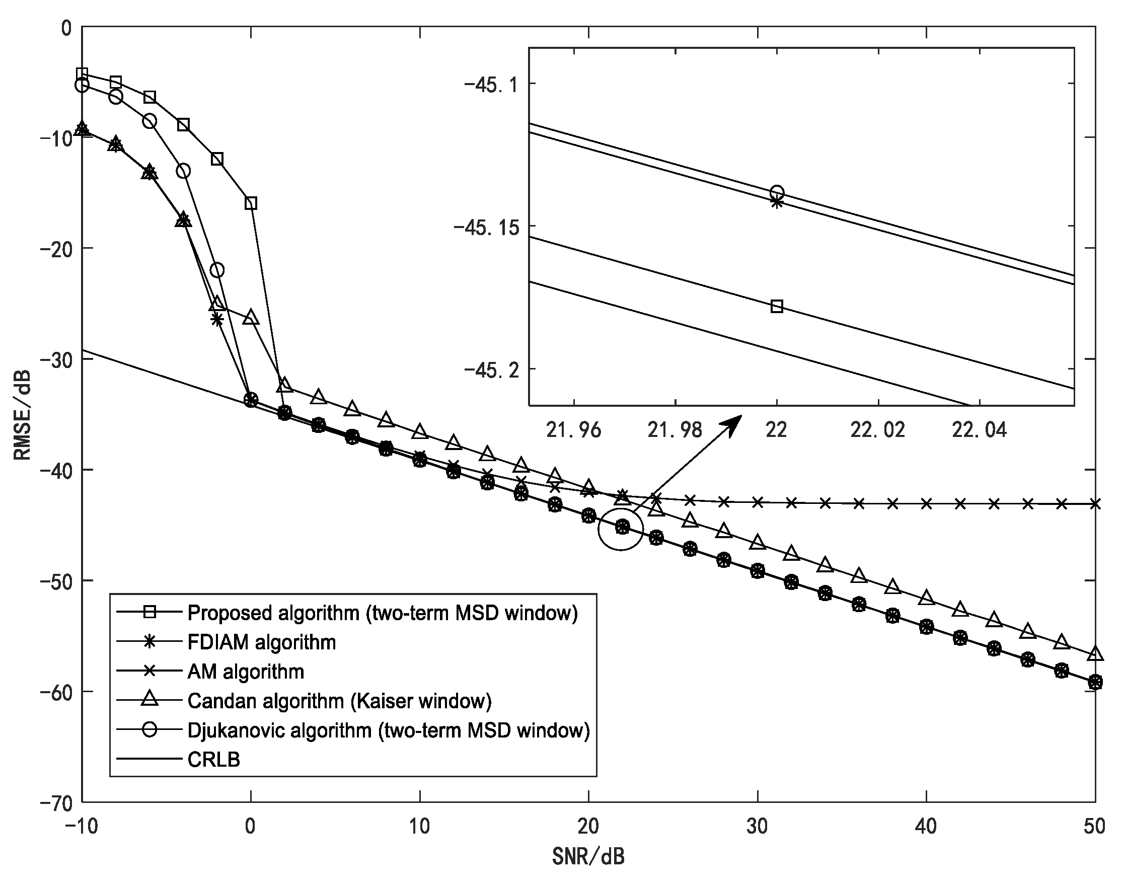
Firstly, we examine the frequency estimation RMSEs of different algorithms versus the SNR in Figure 1. We show the simulation results for $N=128$, $\varphi =\pi /8$, and $f_0=0.1917$. The SNR varies from −10 dB to 50 dB with a step of 2 dB. For each value of SNR, 20,000 time Monte Carlo experiments have been considered. The simulation results of the algorithm we proposed with the three-term MSD window are very similar to those when the signal is multiplied by two-term MSD window. Therefore, only the results of the proposed algorithm with a two-term MSD window are shown. It can be seen that the RMSE of the proposed algorithm with a two-term MSD window is closer to the CRLB than the other methods. The RMSE of the Candan algorithm is clearly larger than that of the other algorithms. When the SNR is higher than 10 dB, the RMSE of the AM algorithm gradually departs from that of the CRLB. Therefore, the accuracy of the proposed algorithm is higher than that of the AM algorithm, Candan algorithm, Djukanovic algorithm, and FDIAM algorithm.

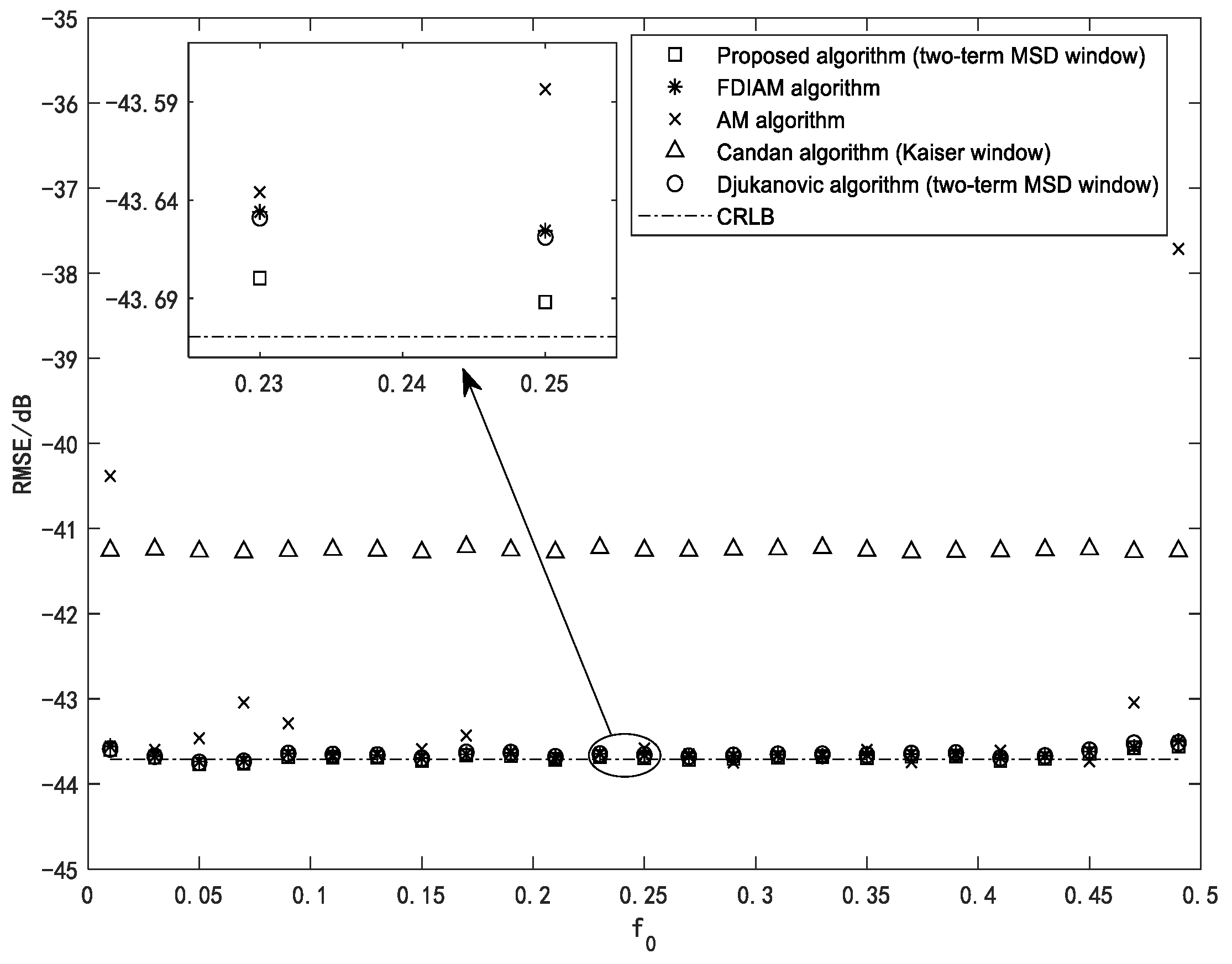
Then, we evaluate the RMSEs of five different algorithms versus the sinusoid frequency $f_0$. We show the simulation results in Figure 2 for $N=256$, $\varphi =\pi /8$, and $SNR=10\mathrm{dB}$. $f_0$ varies in the interval of $\left[0.01,0.49\right]$ with a step of 0.02. For each value of $f_0$, 20,000 time Monte Carlo experiments have been considered. We can see that the RMSE curve of the proposed algorithm is closer to that of CRLB than the other algorithms. Although the Candan algorithm reduces the bias caused by the superposition of the positive and negative frequency spectrum components with Kaiser window, its RMSE is still about 2.5 dB higher than that of the CRLB. The RMSE curve of the AM algorithm fluctuates greatly. Therefore, the accuracy of the proposed algorithm is the highest among all the five estimators. The proposed algorithm is not sensitive to the signal frequency.

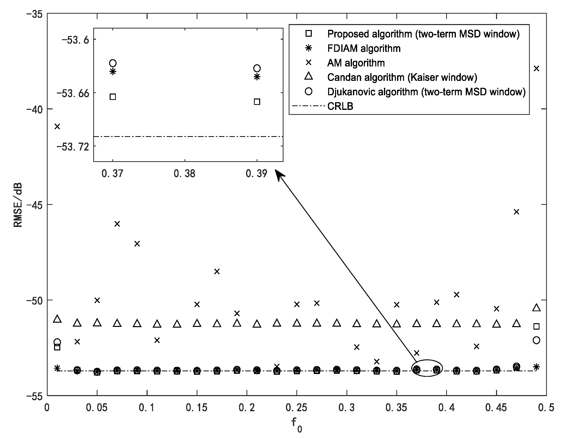
Figure 3 shows the RMSEs of five different estimators versus the sinusoid frequency $f_0$ for, $SNR=30\mathrm{dB}$ and the other parameters remain unchanged, as shown in Figure 2. For each value of $f_0$, 20,000 time Monte Carlo experiments have been considered. We can see that the performance of the AM algorithm is still poor and that its RMSE is large. The RMSE of the Candan algorithm with a Kaiser window is about 2.5 dB higher than that of the CRLB, and the RMSEs of the other three algorithms are fairly small. From the partially enlarged image, we can see that the RMSE of the proposed algorithm is smaller than that of the Djukanovic algorithm and FDIAM algorithm, except when $f_0$ is very close to 0 and 0.5. The proposed algorithm is not sensitive to the signal frequency, except for the cases when $f_0$ is very close to 0 and 0.5.

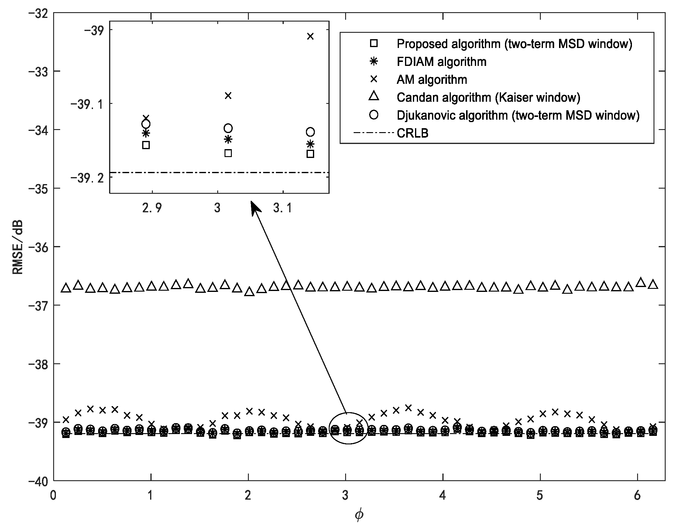
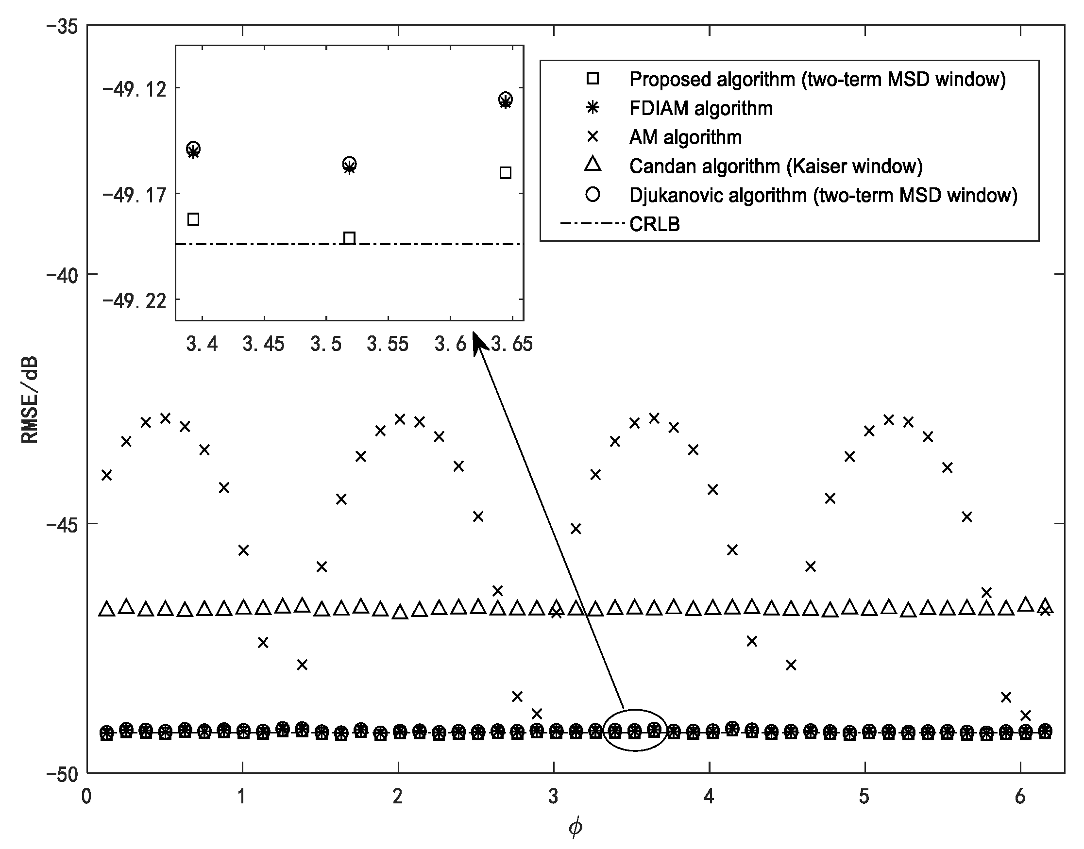
Finally, we evaluate the RMSEs of different algorithms versus the initial phase $\varphi$ for $N=128$, $f_0=0.1917$, and $SNR=10\mathrm{dB}$ in Figure 4. $\varphi$ varies in the range $\left(0,2\pi \right)$ with a step of $\left(1/25\pi \right)$. For each value of $\varphi$, 20,000 time Monte Carlo experiments have been considered. We can see that the Candan algorithm has the largest RMSE among all the estimators. The RMSE of the AM algorithm changes periodically and is higher than the RMSE of the Djukanovic algorithm, the FDIAM algorithm, and the proposed algorithm. From the partially enlarged figure, we can see that the performance of the proposed algorithm is better than that of the other algorithms. The proposed algorithm is not sensitive to the initial phase.

When $SNR=30\mathrm{dB}$ and the other parameters maintain unchanged, as shown in Figure 4, the RMSEs of different estimators versus initial phase $\varphi$ are shown in Figure 5. For each value of $\varphi$, 20,000 time Monte Carlo experiments have been considered. We can see that the accuracy of the proposed estimator is the highest among all the estimators, and the proposed estimator is not sensitive to the initial phase. The RMSE of the AM algorithm still changes periodically and is relatively large. The RMSE of the Candan algorithm is about 2.5 dB higher than that of the CRLB.

We suppose that N-point Fast Fourier Transform (FFT) requires $N{\log }_{2}N$ complex multiplications and complex additions. We also ignore all operations of O (1) complexity, where O (·) represents the big O notation. Then, the proposed algorithm has the same complexity order $O(N{\log }_{2}N)$ as the AM algorithm, Candan algorithm, Djukanovic algorithm, and FDIAM algorithm [24,28].

4. Conclusions

An accurate frequency estimator for a real sinusoid based on DFT is proposed. The proposed estimator is based on the interpolation of the maximum DFT spectral line and two DTFT spectral lines and can operate with both the rectangular window and the MSD window. In the coarse estimation step, the proposed estimator with the MSD window is used. According to the value of the coarse estimate, the negative frequency spectral component is removed. In the fine estimation step, the proposed estimator with the rectangular window is utilized to achieve the CRLB. Computer simulation results show that the estimation accuracy of the presented algorithm is higher than that of the AM algorithm, Candan algorithm, Djukanovic algorithm, and FDIAM algorithm. The presented algorithm is not sensitive to the initial phase and signal frequency in most situations. The presented algorithm has the same computational complexity order as the competing estimators. Therefore, the presented algorithm can reduce the estimation bias caused by the superposition of the positive and negative frequency spectrum components of a real sinusoid. In future research, we will focus on improving the estimation accuracy for extremely small and large values of signal frequency.

References

- Morelli, M.; Moretti, M. A robust maximum likelihood scheme for PSS detection and integer frequency offset recovery in LTE Systems. IEEE Trans. Wirel. Commun. 2016, 15, 1353–1363. [Google Scholar] [CrossRef]
- Liu, S.; Zhang, H.; Shan, T.; Huang, Y. Efficient radar detection of weak maneuvering targets using a coarse-to-fine strategy. IET Radar Sonar Nav. 2021, 15, 181–193. [Google Scholar] [CrossRef]
- Bellili, F.; Selmi, Y.; Affes, S.; Ghrayeb, A. A low-cost and robust maximum likelihood joint estimator for the Doppler spread and CFO parameters over flat-fading Rayleigh channels. IEEE Trans. Commun. 2017, 65, 3467–3478. [Google Scholar] [CrossRef]
- Kim, M. Analysis of Multipath Component Parameter Estimation Accuracy in Directional Scanning Measurement. IEEE Antennas Wirel. Propag. Lett. 2018, 17, 12–16. [Google Scholar] [CrossRef]
- Ding, Y.; Lei, C.; Xu, X.; Sun, K.; Wang, L. Human micro-Doppler frequency estimation approach for Doppler radar. IEEE Access 2018, 6, 6149–6159. [Google Scholar] [CrossRef]
- Chen, T.; Braga-Neto, U.M. Maximum-Likelihood Estimation of the Discrete Coefficient of Determination in Stochastic Boolean Systems. IEEE Trans. Signal Process. 2013, 61, 3880–3894. [Google Scholar] [CrossRef]
- Agüero, J.C.; Yuz, J.I.; Goodwin, G.C.; Delgado, R.A. On the equivalence of time and frequency domain maximum likelihood estimation. Automatica 2010, 46, 260–270. [Google Scholar] [CrossRef]
- Tu, Y.Q.; Shen, Y.L. Phase correction autocorrelation-based frequency estimation method for sinusoidal signal. Signal Process. 2017, 130, 183–189. [Google Scholar] [CrossRef]
- Cao, Y.; Wei, G.; Chen, F.J. An exact analysis of Modified Covariance frequency estimation algorithm based on correlation of single-tone. Signal Process. 2012, 92, 2785–2790. [Google Scholar] [CrossRef]
- Alku, P.; Pohjalainen, J.; Vainio, M.; Laukkanen, A.M.; Story, B.H. Formant frequency estimation of high-pitched vowels using weighted linear prediction. JASA 2013, 134, 1295–1313. [Google Scholar] [CrossRef] [Green Version]
- Nandi, S. Estimation of parameters of two-dimensional sinusoidal signal in heavy-tailed errors. J. Stat. Plan. Inference 2012, 142, 2799–2808. [Google Scholar] [CrossRef]
- Fan, L.; Qi, G.Q. Frequency estimator of sinusoid based on interpolation of three DFT spectral lines. Signal Process. 2018, 144, 52–60. [Google Scholar] [CrossRef]
- Belega, D.; Petri, D. Frequency estimation by two- or three-point interpolated Fourier algorithms based on cosine windows. Signal Process. 2015, 117, 115–125. [Google Scholar] [CrossRef]
- Belega, D.; Petri, D. Sine-wave parameter estimation by interpolated DFT method based on new cosine windows with high interference rejection capability. Digit. Signal Process. 2014, 33, 60–70. [Google Scholar] [CrossRef]
- Fan, L.; Qi, G.Q.; Liu, J.Y.; Jin, J.Y.; Liu, L.; Xing, J. Frequency estimator of sinusoid by interpolated DFT method based on maximum sidelobe decay windows. Signal Process. 2021, 186, 108125. [Google Scholar] [CrossRef]
- Serbes, A. Fast and efficient sinusoidal frequency estimation by using the DFT coefficients. IEEE Trans. Commun. 2019, 67, 2333–2342. [Google Scholar] [CrossRef]
- Aboutanios, E.; Mulgrew, B. Iterative frequency estimation by interpolation on Fourier coefficients. IEEE Trans. Signal Process. 2005, 53, 1237–1242. [Google Scholar] [CrossRef]
- Candan, C. Analysis and further improvement of fine resolution frequency estimation method from three DFT samples. IEEE Signal Process. Lett. 2013, 20, 913–916. [Google Scholar] [CrossRef]
- Fang, L.; Duan, D.; Yang, L. A new DFT-based frequency estimator for single-tone complex sinusoidal signals. In Proceedings of the Military Communications Conference, Orlando, FL, USA, 29 October–1 November 2012; pp. 1–6. [Google Scholar] [CrossRef]
- Zhang, H.; Shan, T.; Liu, S.; Tao, R. Performance evaluation and parameter optimization of sparse Fourier transform. Signal Process. 2021, 179, 107823. [Google Scholar] [CrossRef]
- Candan, C. Fine resolution frequency estimation from three DFT samples: Case of windowed data. Signal Process. 2015, 114, 245–250. [Google Scholar] [CrossRef]
- Dutra, A.; Oliveira, J.D.; Thiago, D.; Netto, S.L.; Silva, E. High-precision frequency estimation of real sinusoids with reduced computational complexity using a model-based matched-spectrum approach. Digit. Signal Process. 2014, 34, 67–73. [Google Scholar] [CrossRef]
- Mikluc, D.; Bujakovic, D.; Andric, M.; Simic, S. Estimation and Extraction of Radar Signal Features Using Modified B Distribution and Particle Filters. Frequenz 2016, 70, 417–427. [Google Scholar] [CrossRef]
- Djukanović, S. An Accurate Method for Frequency Estimation of a Real Sinusoid. IEEE Signal Process. Lett. 2016, 23, 915–918. [Google Scholar] [CrossRef]
- Ye, S.; Kocherry, D.L.; Aboutanios, E. A novel algorithm for the estimation of the parameters of a real sinusoid in noise. In Proceedings of the 23rd European Signal Processing Conference, Nice, France, 31 August–4 September2015; pp. 2271–2275. [Google Scholar]
- Wang, K.; Tu, Y.; Mclernon, D.; Shen, Y.; Chen, P. A spectrum matching method for accurate frequency estimation of real sinusoids. Rev. Sci. Instrum. 2019, 90, 045112. [Google Scholar] [CrossRef]
- Candan, C.; Çelebi, U. Frequency estimation of a single real-valued sinusoid: An invariant function approach. Signal Process. 2021, 185, 108098. [Google Scholar] [CrossRef]
- Ye, S.; Sun, J.; Aboutanios, E. On the estimation of the parameters of a real sinusoid in noise. IEEE Signal Process. Lett. 2017, 24, 638–642. [Google Scholar] [CrossRef]
- Liu, Z.H.; Fan, L.; Liu, J.Y.; Liu, N.; Jin, J.Y.; Xing, J. Accurate Frequency Estimator of Real Sinusoid Based on Maximum Sidelobe Decay Windows. In Proceedings of the 16th EAI ChinaCom 2021 Conference, Beijing, China, 21–22 November 2021; pp. 40–51. [Google Scholar] [CrossRef]
Figure 1.
RMSEs versus SNR for , , and .
Figure 2.
RMSEs versus for , , and .
Figure 3.
Figure 4.
Figure 5.