the Creative Commons Attribution 4.0 License.
the Creative Commons Attribution 4.0 License.
 | 23 Sep 2022
Northern hemispheric atmospheric ethane trends in the upper troposphere and lower stratosphere (2006–2016) with reference to methane and propane
Andrea Pozzer
Jos Lelieveld
Jonathan Williams
Methane, ethane, and propane are among the most abundant hydrocarbons in the atmosphere. These compounds have many emission sources in common and are all primarily removed through OH oxidation. Their mixing ratios and long-term trends in the upper troposphere and stratosphere are rarely reported due to the paucity of measurements. In this study, we present long-term (2006–2016) northern hemispheric ethane, propane, and methane data from airborne observation in the upper troposphere-lower stratosphere (UTLS) region from the IAGOS-CARIBIC project. The methane and propane observations provide additional information for understanding northern hemispheric ethane trends, which is the major focus of this study. The linear trends, moving averages, nonlinear trends and monthly variations of ethane, methane and propane in 2006–2016 are presented for the upper troposphere and lower stratosphere over 5 regions (whole Northern Hemisphere, Europe, North America, Asia and the rest of the world). The growth rates of ethane, methane, and propane in the upper troposphere are −2.24 % yr−1, 0.33 % yr−1, and −0.78 % yr−1, respectively, and in the lower stratosphere they are −3.27 % yr−1, 0.26 % yr−1, and −4.91 % yr−1, respectively, in 2006–2016. This dataset is of value to future global ethane budget estimates and the optimization of current ethane inventories. The data are publicly accessible at https://doi.org/10.5281/zenodo.6536109 (Li et al., 2022a).
- Article
(6791 KB) - Full-text XML
-
Supplement
(1825 KB) - BibTeX
- EndNote


Ethane (C2H6) is among the most abundant non-methane hydrocarbons (NMHC) present in the atmosphere. Major sources of ethane to the atmosphere are via natural gas and oil production (∼ 62 %), biofuel combustion (20 %), and biomass burning (18 %). Interestingly, 84 % of the total emissions are from the Northern Hemisphere (NH) (Xiao et al., 2008). Oxidation by hydroxyl (OH) radicals is the major atmospheric loss process for tropospheric ethane, while in the stratosphere the reaction with chlorine (Cl) radicals provides an additional loss process (Li et al., 2018). Due to the seasonal variation of ethane emissions and the photochemically generated OH radicals, ethane has a clear annual cycle in mole fractions, showing higher levels in winter. Its global lifetime is circa 3 months, with a minimum in summer (∼ 2 months) and a maximum in winter (∼ 10 months) (Xiao et al., 2008; Helmig et al., 2016; Li et al., 2018). Ethane oxidation forms acetaldehyde, which in turn contributes to the formation of peroxyacetyl nitrate (PAN) or peracetic acid depending on the levels of NOx (Millet et al., 2010). The PAN acts as a reservoir species of nitrogen oxides (NOx) and can strongly affect tropospheric ozone distributions by transporting NOx from the point of emission to remote locations. Furthermore, PAN is known to be a secondary pollutant like ozone with negative impacts on regional air quality and human health (Rudolph, 1995; González Abad et al., 2011; Fischer et al., 2014; Monks et al., 2018; Kort et al., 2016; Tzompa-Sosa et al., 2017; Dalsøren et al., 2018; Pozzer et al., 2020).
Many studies have reported ethane trend analyses based on either ground-based sampling or Fourier transform infrared spectrometer (FTIS) measurements. A summary of these studies is shown in Table 1. In the troposphere (Table 1a), a decreasing trend of ethane during 1986–2008 and an increasing trend during 2009–2014 were reported in the literature. The trends of C2H6 partial column at four European sites (Jungfraujoch, Zugspitze, Harestua and Kiruna) during 1996–2006 were between about −1.09 % yr−1 to −2.11 % yr−1 (Angelbratt et al., 2011). Simpson et al. (2012) concluded a strong global ethane decline of 21 % over 26 years (1984–2010), with a stronger decline occurring from 1984 to 1999 (−7.2 ± 1.7 ppt yr−1) than from 2000 to 2010 (−1.9 ± 1.3 ppt yr−1). Franco et al. (2015) showed the ethane trend at Jungfraujoch to be −0.92 % yr−1 during 1994–2008, followed by a strong positive trend of 4.9 % yr−1 during 2009–2014, which may be related to the intensifying emissions from shale gas exploitation in North America. Helmig et al. (2016) calculated a mean ethane growth rate of 2.9 % yr−1–4.7 % yr−1 from 2009 to 2014 at 32 NH ground measurement sites and concluded that North American oil and gas development was the primary source of the increasing emission of ethane. Franco et al. (2016) compared the ethane total column change at six sites across NH for the periods of 2003–2008 and 2009–2014, and also revealed a sharp increase of 3 % yr−1–5 % yr−1 during 2009–2014 compared with 2003–2008, which was associated with oil and gas industry emissions. Hausmann et al. (2016) presented a positive ethane trend of ca. 4.6 % yr−1 at Zugspitze (47∘ N) and a negative trend of ca. −2.5 % yr−1 at Lauder (45∘ S) for 2007–2014, and inferred an ethane increase from oil and gas emissions of 1–11 Tg yr−1 for 2007–2014. Angot et al. (2021) showed an increasing trend in ethane of ca. 5.6 % yr−1 at GEOSummit (73∘ N) for 2010–2014, followed by a temporary pause of ethane growth in 2015–2018. Sun et al. (2021) presented a negative ethane trend of −2.6 ± 1.3 % yr−1 over 2015–2020 in the densely populated eastern Chinese city Hefei.
Table 1Summary of studies reporting ethane trends in the (a) troposphere and (b) stratosphere. Parentheses in first column indicate the locations of measurements.
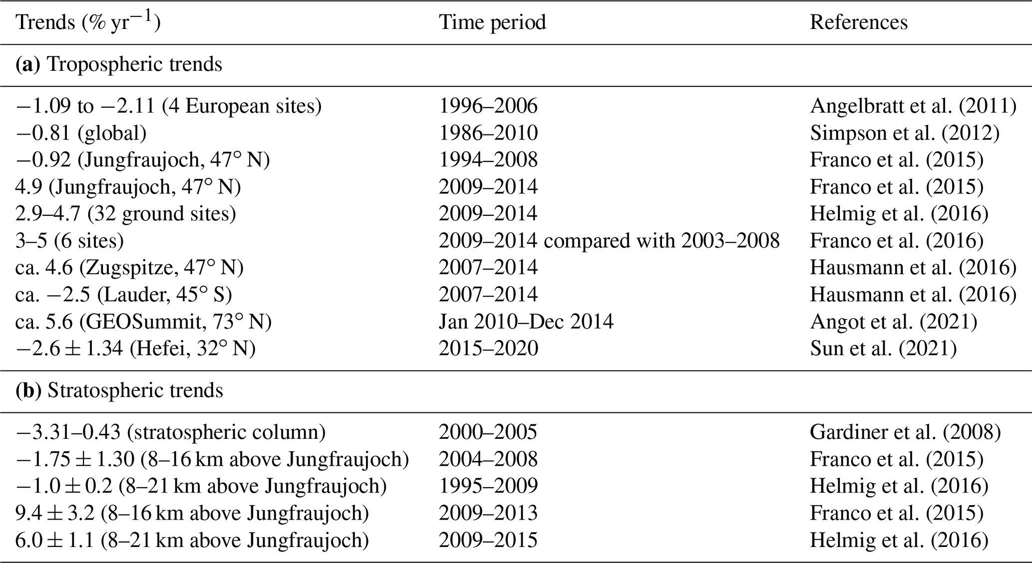
In contrast to tropospheric ethane trends, trends in the stratosphere have been far less investigated. The stratospheric ethane trends were reported to follow a decreasing trend in 1995–2008 and an increasing trend in 2009–2015 (Table 1b). Gardiner et al. (2008) presented the annual trend in stratospheric ethane column (relative to year 2000) at 6 sites and these varied from 0.43 to −3.31 % yr−1 until the year 2005. Franco et al. (2015) reported ethane trends at 8–16 km measured at Jungfraujoch of −1.75 ± 1.30 % yr−1 for 2004–2008 and 9.4 ± 3.2 % yr−1 for 2009–2013, indicating an ∼ 11 % sharp increase since 2009. Helmig et al. (2016) showed that the UTLS column ethane (8–21 km) measured at Jungfraujoch was decreasing by −1.0 ± 0.2 % yr−1 from 1995 to 2009, and started a sharp increase at a rate of 6.0 ± 1.1 % yr−1 from 2009 until 2015, while the difference in growth rate between the two time periods was smaller for the mid-tropospheric column (3.6–8 km): −0.8 ± 0.3 % yr−1 (1995–2009) and 4.2 ± 1.0 % yr−1 (2009–2015).
Previous investigations of the distribution, emissions, lifetime, and atmospheric trends of ethane have been mostly based on surface-based measurements. These have been either from a regionally focused intensive field measurement campaign (e.g., Kort et al., 2016) or from networks of remote sampling stations (e.g., Franco et al., 2015; Helmig et al., 2016). The advantage of surface sites is that they are easily accessed and maintained; however, such measurements inevitably reflect the local or regional situation, and changes in emissions immediately upwind of a measurement location can affect the results, masking any underlying long-term global trends. In addition, most ethane measurement sites are located in high-income countries, such as North America and Europe, while ethane observations in the rest of the world are sparse. This too hinders the assessment of global ethane trends, for while one country's emission may be declining another's could be rapidly increasing. For the aforementioned reasons, it is advantageous to assess the global long-term ethane trend from the upper troposphere and even the stratosphere where emissions can be expected to be well-mixed by atmospheric circulation. In particular, the trend of ethane in the more isolated and remote stratosphere is of interest when assessing long-term changes.
In this study, we use airborne observations covering the Northern Hemisphere (NH), including regions without ground measurements. We present long-term northern hemispheric and geographically delineated (North America, Asia, Europe, rest of the world) ethane trends in the upper troposphere and lower stratosphere for the decade 2006–2016 derived using airborne measurements. In addition, the trends of methane and propane collected from the same observations are examined to better understand the observed variation of NH ethane trends, as they have common sources and sinks in the atmosphere. This study focuses on describing the dataset itself, therefore, an in depth interpretation is outside the scope. All the data used in this study are publicly available at https://doi.org/10.5281/zenodo.6536109 (Li et al., 2022a). These data can be used for further analysis on global and regional trends, emissions and lifetime of methane, ethane, and propane, their contributions to climate change, troposphere-stratosphere exchange, and improvement of current inventories and atmospheric models.
2.1 IAGOS-CARIBC observations
The In-service Aircraft for a Global Observing System-Civil Aircraft for the Regular Investigation of the atmosphere Based on an Instrument Container (IAGOS-CARIBIC) project is an aircraft-based scientific project with the aim of monitoring long-term global atmospheric physics and chemistry (Brenninkmeijer et al., 2007). The flight altitudes are at ∼ 10 km, which is in the upper troposphere-lower stratosphere (UTLS) region. A custom-built whole air sampler collects pressurized air samples during each flight, and these samples are subsequently measured in the laboratory with gas chromatography (GC) coupled with three detectors: GC-ECD (for carbon dioxide, nitrous oxide, and sulfur hexafluoride) (Schuck et al., 2009), GC-FID for methane and volatile organic compounds (including ethane and propane) (Baker et al., 2010), and GC-AED for volatile organic compound measurements after 2017 (data not used in this study) (Karu et al., 2021). The precision of ethane and propane data used in this study is 0.2 % and 0.8 %, respectively (Baker et al., 2010), and of methane 0.17 % (Schuck et al., 2009). Details regarding operational and analytical procedures, calibration scales, and quality assurance are documented in the cited references, and summarized as follows:
Each IAGOS-CARIBIC flight normally consists of 4 flight sequences with a total number of 116 air samples collected by whole air samplers (flasks). The inlet and outlet of each flask are connected by multiposition valves which can be automatically switched with programming. A pumping system and pressure sensors are connected to the inlet valves to guarantee the final pressure in each flask to be around 4.5 bar. The outlet valves are connected to ambient air. Prior to pressurization, each flask is flushed with ambient air 10 times (about 5–10 min). The average filling (sampling) time of each flask is about 45 s (range 0.5–1.5 min) depending on the flight altitude, resulting a spatial resolution of 7–21 km.
Methane (CH4), ethane (C2H6), and propane (C3H8) were measured with an HP 6890 GC with a polymer Porapak Q 3/4” column (10 ft, 100/120 mesh) installed in a single oven. Nitrogen (N2, purity 99.999 %) was used as carrier gas at a constant flow rate of 50 mL min−1. The GC was operated at an oven temperature of 220 ∘C with flow rates of synthetic air of 250 mL min−1 and hydrogen of 80 mL min−1. Water vapor in samples was removed by passing through a drying tube at the start of the analysis. The calibration standards and reference gas cylinders were ordered from NOAA (for methane), and the National Physical Laboratory (for ethane and propane) which are certified against the World Meteorological Organization (WMO) Global Atmosphere Watch (GAW) program scale, and they are regularly renewed within every 3 years, which guarantees the stability of calibration gases. Three additional calibration standards samples were measured between samples of each flight sequence in order to monitor the quality of measurements and reduce uncertainty.
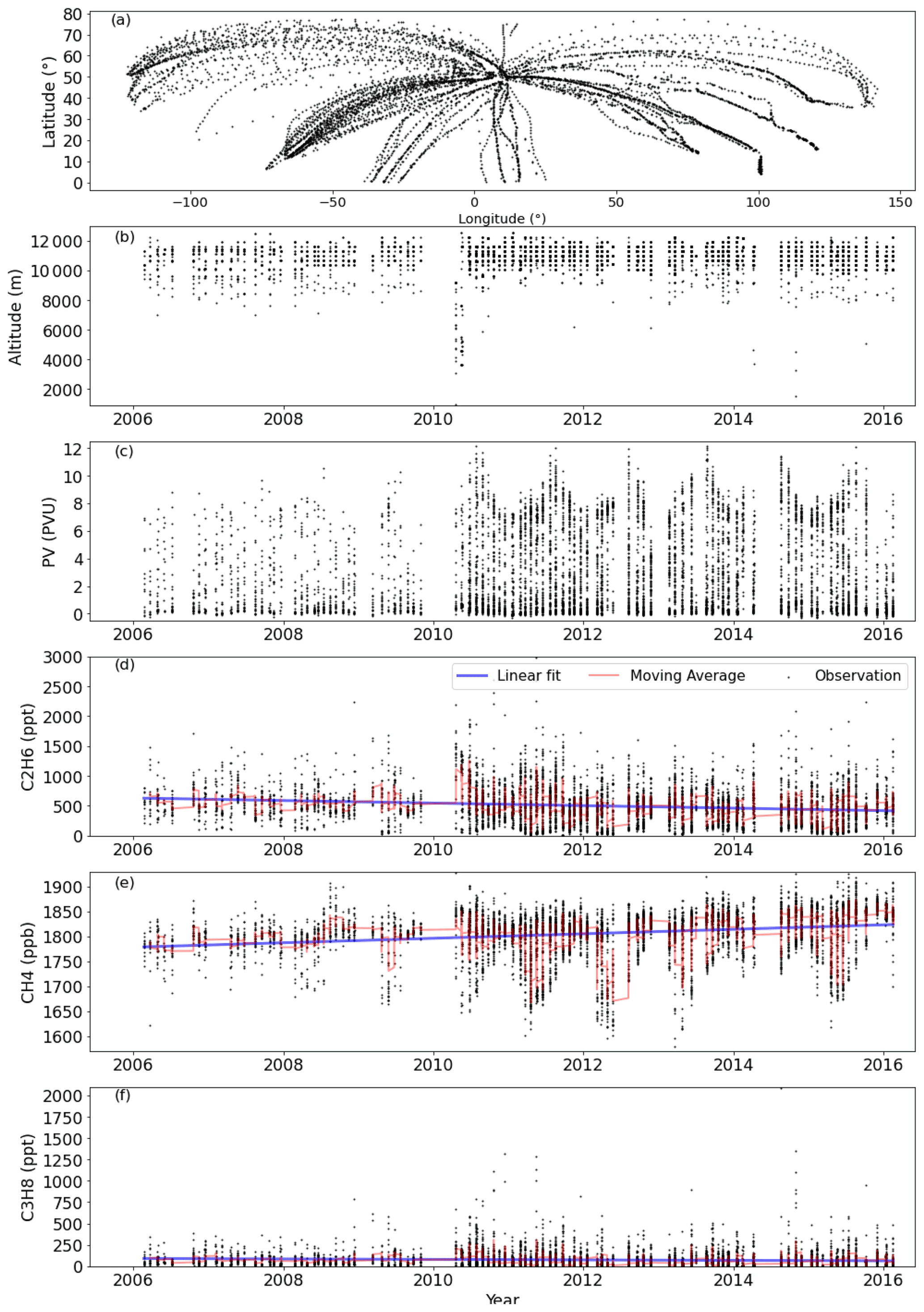
Figure 1Data overview of (a) geographical distribution, (b) altitude, (c) potential vorticity (PV), mole fractions of (d) ethane, (e) methane and (f) propane.
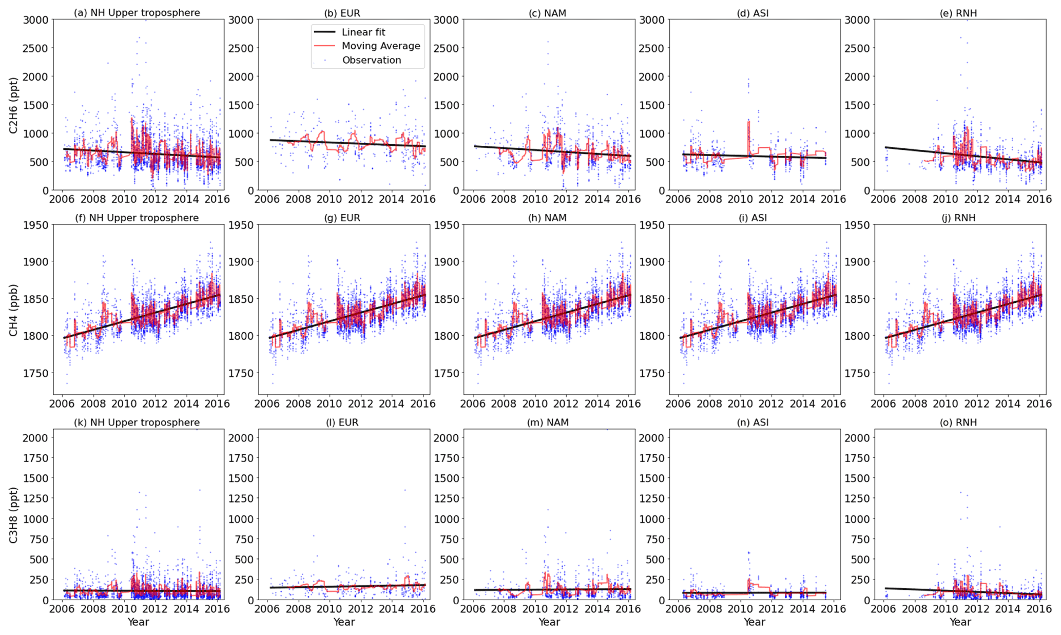
Figure 2The upper tropospheric ethane, methane and propane mole fractions from observations and linear trends over five regions, whole NH upper troposphere, EUR, NAM, ASI, and RNH.
In total 6607 NH samples were collected during February 2006–February 2016. The overview of geographical distribution, altitude, PV, ethane, methane and propane of all 6607 samples collected in 2006–2016 is shown in Fig. 1. Samples were collected in a broad range of latitudes (0.2–77.4∘) and longitudes (−122.2–141.8∘) (Fig. 1a). Of the samples 57.9 % were collected in the latitude bands of 30–60∘, 25.6 % were from latitudes 0–30∘, and 16.5 % from latitudes above 60∘. Samples were collected at an altitude range of 946.4–12,525.1 m, with 98.8 % being collected above 8000 m (Fig. 1b). The PV values of all the samples ranged from −0.32 to 12.17 (Fig. 1c). For the trend analyses in the later sections, samples collected at altitudes lower than 8000 m and PV <2 PVU were excluded, 74 samples were collected at altitudes lower than 8000 m and a potential vorticity (PV) <2 potential vorticity unit (PVU), where they can be largely influenced by surface emissions. Therefore, those samples were excluded from trend analyses. The remaining 6533 samples were divided into two categories: upper tropospheric samples (altitude ≥8000 m and PV <2 PVU), and lower stratospheric samples (PV ≥2 PVU). To investigate the changes above the tropopause, the lower stratospheric samples were classified into the lower part of the lower stratosphere (2 PVU ≤ PV <6 PVU) and the upper part (PV ≥6 PVU). All samples were categorized into four regions based on their sampling locations: North America (NAM), Asia (ASI), Europe (EUR), and rest of Northern Hemisphere (RNH). The coordinates of each region are shown in Table S1 (in the Supplement) and the geographical distribution of samples is shown in Fig. S1 (in the Supplement). In later analyses we used the term “whole NH” to refer to the combination of all four regions. Table 2 shows the total sample number collected in 2006–2016 of 20 subregions, i.e., 4 categories (upper troposphere, lower stratosphere, lower stratosphere-lower part, lower stratosphere-upper part) and 5 regions (whole NH, EUR, NAM, ASI, RNH). The later sections will further investigate the trends and seasonality of ethane, methane and propane in these 20 subregions. It is noted that the region designated does not correspond to the source region, only the geographical location of the data points.
Table 2Sample number and linear trends of ethane, methane and propane.
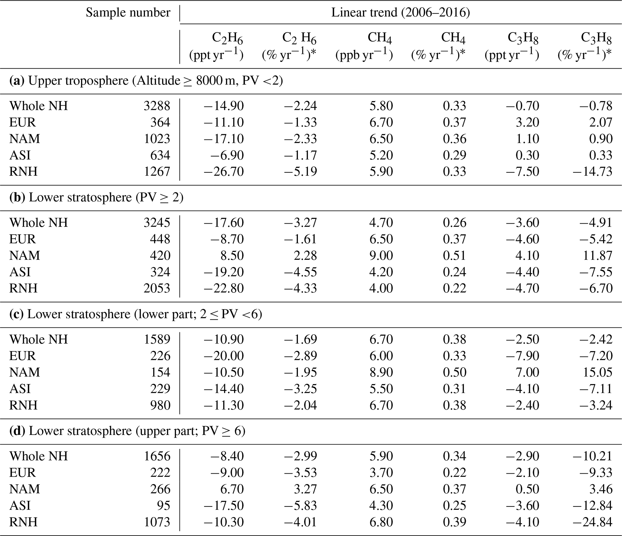
* Growth rate relative to rolling average of first 20 observations of the dataset of each region.
2.2 Trend analysis
We have applied three trend analysis methods in this study: linear fit, moving average, and nonlinear trend.
Linear fit was applied to each subregion throughout the entire time period (2006–2016). The growth rates of ethane, methane and propane of each subregion by linear fit are shown in Table 2. These growth rates are referred as “linear trend” in later sections.
Moving average was achieved with Python (version 3.9.7) pandas package DataFrame.rolling function using a rolling sum with a window length of 20 observations.
Nonlinear trend analysis using the “Prophet” algorithm (Taylor and Letham, 2018). The “Prophet” algorithm has been applied on the analysis of noncontinuous time-series datasets (Li et al., 2022b), as is the case for aircraft data. The trend analysis model has four components: trend (nonperiodic changes), seasonality (periodic changes), holiday effects, and error (idiosyncratic changes). In this study, effects of holidays are not included. We used a linear model with change points for the trend component, and the trend function consists of growth rate, adjustments of growth rate, and offset parameter. The flexibility of trend (e.g., overfitting or underfitting) can be adjusted by the parameter “changepoint_prior_scale”. A change point represents the moments where the data shift directions. The value of the parameter “changepoint_prior_scale” represents the strength of change points, more change points will be automatically detected when the value of this parameter increases. The uncertainty interval was set at 95 %. The code of trend analysis in Python for this study can be found in the Supplement. Figure S2 shows the ethane trend and seasonality at Iceland estimated by the “Prophet” algorithm. Compared with the trend and seasonality estimated by the NOAA algorithm using the same dataset in Fig. 1b of Helmig et al. (2016), the seasonality of ethane is captured by both algorithms and the results match with each other. The nonlinear trend is estimated as the average value of 10 fitting levels on the trend (i.e., “changepoint_prior_scale” = 0.1, 0.2, 0.3, … , 0.9, 1.0).
The uncertainty of the non-linear trend analysis is estimated by resampling methods. For the dataset of each subregion, we randomly resampled the dataset 20 times, with each time consisting of 90 % of the samples of the dataset. We then run the “Prophet” algorithm for each of the 20 sub datasets, using the average value of 10 fitting levels as the trend of each subdataset. The range of the 20 trends from the resampled datasets is assumed as the uncertainty of nonlinear trend analysis for each subregion.
3.1 Overview of IAGOS-CARIBC observations
Figure 1d, e, f shows the observed ethane, methane and propane mole fractions, their linear trends over 2006–2016, and their moving average. The observed mole fractions of ethane, methane and propane are in the range of 5.5–2982.2 ppt, 1579.7–1926.8 ppb, and 1.0–2090.0 ppt, respectively. Both ethane and propane showed decreasing trends using linear fit over 2006–2016, and methane had an increasing growth rate over the same period. The exact growth rates of ethane, methane, and propane are not reported here; however, they are reported in the later sections where regional trends are investigated.
3.2 Upper tropospheric trends
3.2.1 Linear trends in the upper troposphere
Figure 2 shows the upper tropospheric observations, linear trends and moving average of ethane (Fig. 2a, b, c, d, e), methane (Fig. 2f, g, h, i, j) and propane (Fig. 2k, l, m, n, o) over five regions: the whole Northern Hemisphere (Fig. 2a, f, k), Europe (Fig. 2b, g, l), North America (Fig. 2c, h, m), Asia (Fig. 2d, i, n), and the rest of the world (Fig. 2e, j, o). The growth rates of ethane, methane and propane over each region are shown in Table 2a.

Figure 3Nonlinear trends of the upper tropospheric ethane, methane and propane over five regions (whole NH upper troposphere, EUR, NAM, ASI, and RNH).
The upper tropospheric ethane shows decreasing trends over all regions for 2006–2016, with the most decrease in RNH (−26.7 ppt yr−1, −5.19 % yr−1) and the least decrease in ASI (−6.9 ppt yr−1, −1.17 % yr−1). The whole NH upper tropospheric ethane decreased at a rate of −14.9 ppt yr−1 (−2.24 % yr−1) over 2006–2016. Unlike the large variations in linear trends of ethane among regions, the upper tropospheric methane shows more homogeneous increasing trends among all regions (range 5.2–6.7 ppb yr−1, 0.29–0.37 % yr−1) due to its longer atmospheric lifetime. The whole NH upper tropospheric propane decreased at a rate of −0.7 ppt yr−1 (−0.78 % yr−1), which is dominated by the decrease in RNH (−7.5 ppt yr−1, 14.7 % yr−1). The upper tropospheric propane mole fractions were increasing at rates of 0.3–3.2 ppt yr−1 (0.33–2.1 % yr−1) in EUR, ASI and NAM.
3.2.2 Nonlinear trends in the upper troposphere
The nonlinear trends of upper tropospheric ethane, methane, and propane at regional scales, estimated by the “Prophet” algorithm and their associated uncertainties are shown in Fig. 3. Ethane and methane share common sources in gas and oil emissions, and ethane, methane, and propane react with OH radicals as their major sinks in the troposphere.
In early 2010, a peak is clearly seen for all three compounds in the whole NH upper troposphere, which may indicate a decrease in OH radicals. This peak is also pronounced in ASI for all three compounds; however, the methane peak in ASI has a large uncertainty.
Ethane and propane in EUR are noticeably higher than other regions due to lower sampling altitudes in EUR (Fig. S3, mean ± 1 standard deviation, 10 197 ± 857 m) compared to other regions (NAM: 10 982 ± 557 m; ASI: 10 621 ± 942 m; RNH: 11 054 ± 580 m), whereas methane in EUR is at a similar level to other regions due to methane's longer atmospheric lifetime.
Large uncertainties occur when the sampling number was low (<100). For example, the trend uncertainties for ethane, methane and propane in ASI were large during January 2009–November 2011, because most ASI samples were collected during June–October 2010, and there was a 1.5 year gap between January 2009 and June 2010 when no samples were collected (Fig. 2).
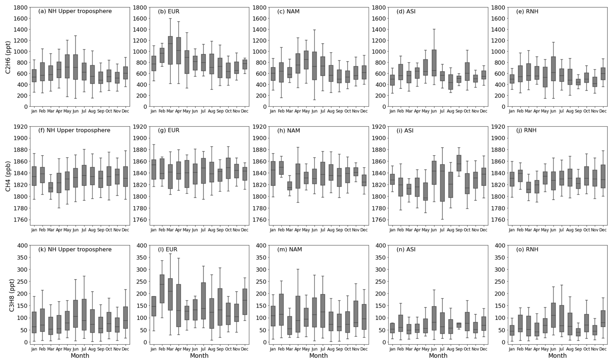
Figure 4Monthly variations of the upper tropospheric ethane, methane and propane (2006–2016) over five regions (whole NH, EUR, NAM, ASI and RNH). The boxes represent 25 %–75 % of all observed mole fractions, the horizontal lines in the boxes indicate the medians. The whiskers represent the 10 %–90 % range of all the observed mole fractions.
3.2.3 Monthly variation in the upper troposphere
The monthly variations of the observed upper tropospheric ethane, methane and propane mole fractions (2006–2016) over five regions (whole NH, EUR, NAM, ASI and RNH) are shown in Fig. 4. The observed monthly variations are driven by the emissions and atmospheric hydroxyl radical (OH) cycle (the major sink for tropospheric ethane, methane and propane). The whole NH upper tropospheric ethane, methane and propane mole fractions show peaks in June and July. The upper tropospheric NAM and EUR ethane mole fractions increase from October and/or November peaking in April and decrease from April until October. This is consistent with the FTIR observation (Franco et al., 2015). The upper tropospheric ASI and RNH ethane peaks in June, 2 months later than NAM and EUR. Methane shows small monthly variations in EUR, NAM and RNH, suggesting that the emissions play a greater role and thus compensate the influence of the seasonal cycle of the OH radical. The upper tropospheric methane in ASI has shown higher mole fractions in summer (June–September) due to deep convection of upward transport of surface air with higher methane into the upper troposphere during Asian monsoons (Baker et al., 2012). The monthly variations of propane are more variable compare to ethane due to the shorter lifetime of propane and probably more variable emission sources of propane.
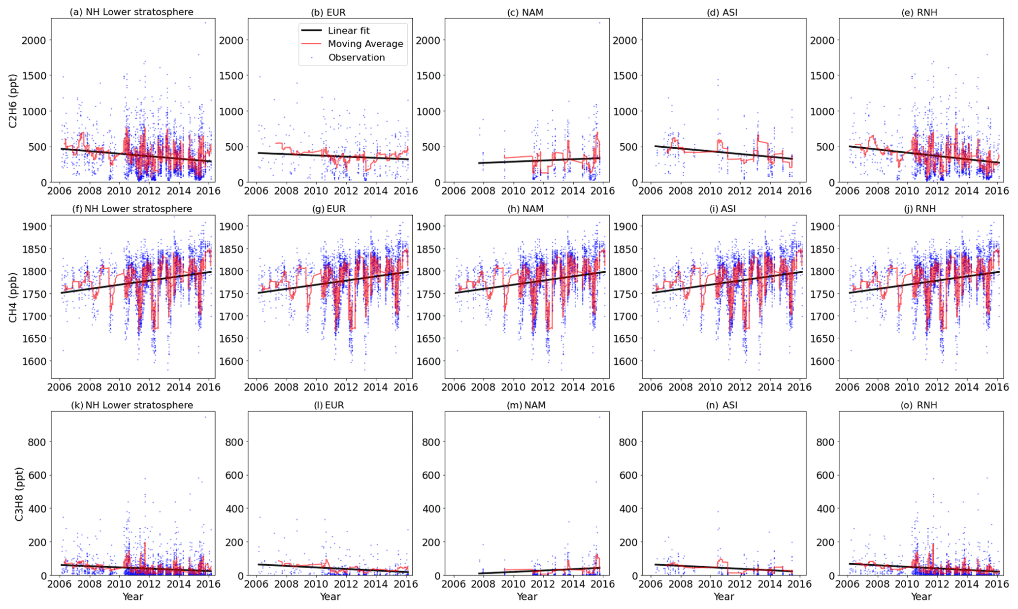
Figure 5Lower stratospheric ethane, methane and propane mole fractions from observations and linear trends over five regions (whole NH lower stratosphere, EUR, NAM, ASI, and RNH).
3.3 Lower stratospheric trends
The sources and sinks of ethane, methane and propane in the stratosphere are different than in the troposphere. There is no known large emission source of ethane, methane and propane in the stratosphere. Stratospheric samples have a wider source footprint and are influenced by troposphere-stratosphere exchange, and chemical reactions. In the stratosphere the OH radical concentration on average decreases by a factor of 10 compared with tropospheric OH levels, whereas halogen radicals, e.g., chlorine (Cl) and bromine (Br), are more abundant and react faster with ethane, methane and propane and therefore play a greater relative role in ethane, methane and propane oxidation (Li et al., 2018). The loss of ethane in the stratosphere by reaction with Cl radicals is about 40 times more than that by OH radicals. The reaction rate of ethane with Cl is about 400 times faster than with OH at 250 K (Atkinson et al., 2006) and stratospheric OH is about 10 times more abundant than stratospheric Cl (Li et al., 2018), whereas the ethane loss in the troposphere by Cl is negligible compared with by OH due to the small amounts of tropospheric Cl (OH:Cl around 10 000) (Lelieveld et al., 1999; Gromov et al., 2018). The reaction rates of ethane, methane and propane with Cl radicals are about at 298 K (Atkinson et al., 1997), indicating that propane and ethane are more sensitive to the changes in stratospheric Cl radicals.
3.3.1 Linear trends in the lower stratosphere
Figure 5 shows the lower stratospheric observations, linear trends and moving average of ethane (Fig. 5a, b, c, d, e), methane (Fig. 5f, g, h, i, j) and propane (Fig. 5k, l, m, n, o) over five regions: the whole Northern Hemisphere (Fig. 5a, f, k), Europe (Fig. 5b, g, l), North America (Fig. 5c, h, m), Asia (Fig. 5d, i, n), and the rest of the world (Fig. 5e, j, o). The growth rates of ethane, methane and propane over each region are shown in Table 2b.
The growth rates of lower stratospheric methane over all five regions (range 0.22 % yr−1–0.51 % yr−1) are consistent with the upper tropospheric methane (range 0.29 % yr−1–0.37 % yr−1) (Table 2). In contrast, the difference between the lower stratospheric and upper tropospheric propane growth rates is large (usually >1.5 % yr−1), because propane has a higher sensitivity to stratospheric chlorine and a shorter lifetime compared to methane. The lower stratospheric ethane has similar growth rates in the whole NH, EUR and RNH compared with the upper troposphere, whereas differences occurs in NAM and ASI. The Asian summer monsoon may be a reason for the different growth rates in ASI, although further investigation on the change in troposphere-stratosphere mixing and stratospheric chlorine in NAM is needed.
3.3.2 Nonlinear trends in the lower stratosphere
The observed lower stratospheric ethane over the whole NH shows two exceptional peaks in 2010 and 2013 (Fig. 6a). The peak in 2010 is not seen at regional levels (NAM, ASI, EUR), which suggests global upward transport of the upper tropospheric ethane (peaking in 2010–2011) into the stratosphere and the important contribution from RNH. The second peak in 2013 can be due to the regional emission transport from the troposphere into the lowermost stratosphere as such a peak is observed simultaneously over NAM, ASI and RNH, or due to changes in stratospheric sinks (e.g., OH or Cl radical concentration) as such peaks are seen for all three compounds.

Figure 6Nonlinear trends of the lower stratospheric ethane, methane and propane over five regions (whole NH lower stratosphere, EUR, NAM, ASI, and RNH).
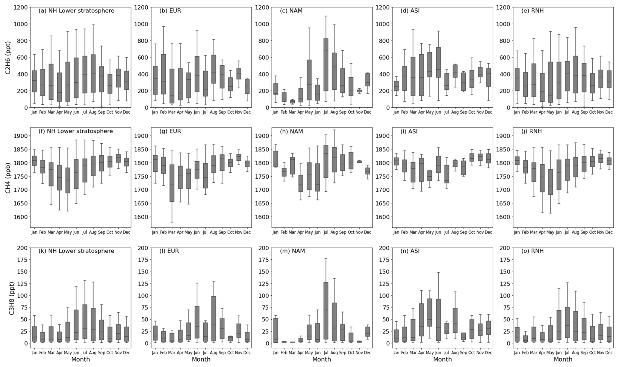
Figure 7Monthly variations of the lower stratospheric ethane, methane and propane (2006–2016) over five regions (whole NH, EUR, NAM, ASI and RNH). The boxes represent 25 %–75 % of all observed mole fractions, the horizontal lines in the boxes indicate the medians. The whiskers represent the 10 %–90 % range of all the observed mole fractions.
Methane trends in the lower stratosphere show large variability during 2010–2014 over the whole NH, ASI and RNH, similar variability is present in the upper tropospheric methane trends (Fig. 3), indicating a fluctuated upwards transport of surface emissions into the upper troposphere and stratosphere.
3.3.3 Monthly variation in the lower stratosphere
The lower stratospheric ethane mole fractions do not show strong seasonality (Fig. 7), except that NAM has a seasonal trend with a 1-month later shift compared to the upper tropospheric NAM trend. The lower stratospheric ASI ethane shows the same timing peak in June with upper tropospheric ASI ethane, which potentially indicates the intrusion of tropospheric air masses into the stratosphere due to Asian summer monsoons (Xiong et al., 2009; Park et al., 2007). There is little seasonality evident in the ethane mole fractions in the stratosphere. Since stratospheric aircraft measurement campaigns are generally of short duration (several weeks), a direct comparison to previous data is not possible; however, vertical column data obtained by ground-based FTIR for 8–21 km reported by Helmig et al. (2016) also showed no clear seasonal variation.
The lower stratospheric methane is observed to reach the lowest in March–May over all five regions. Propane in the lower stratosphere reaches the highest in June–August over most regions except ASI.
3.3.4 Trends in the lower and upper parts of the lower stratosphere
Because the potential vorticity of the lower stratospheric samples has a broad range (2–12.2 PVU), the lower stratosphere is further classified into two parts: lower part (2 ≤ PV <6 PVU) and upper part (PV ≥ 6 PVU), to investigate the changes of trends within the lower stratosphere. It is noted that the sample number of each subregion becomes smaller (95–1656 samples per region; Table 2) by applying this classification, thus the trends have larger uncertainties and should be interpreted with caution.
The linear trends of methane over all five regions, and ethane over four regions (except ASI) show little difference between the lower and upper parts of the lower stratosphere (Table 2c, d; Figs. S4–S5). Larger differences (Delta >2 %) in growth rates of ethane in ASI, and propane over all five regions are found.
The nonlinear trends of ethane, methane and propane in the upper and lower parts of the lower stratosphere are similar over most regions (Figs. S6–S7). A significant difference occurs for ethane in ASI during 2006–2013 when the lower part ethane had a sharp increase in 2006–2007, then followed by a plateau in 2007–2013, whereas the upper part ethane had a continuous decrease in 2006–2013. It is noted that the sample number in upper part of the lower stratosphere over ASI is the minimum among all the subregions (Table 2).
3.4 Limitations and implications
Despite the usefulness, uniqueness and high quality of our datasets, several limitations of our study should be noted. (a) Representativeness of the presented trends. Although our flight sampling is frequent and covers a large area of the NH, the spatial and temporal distributions of our samples are not even. This may cause the trends to be influenced by specific regions where more samples were collected. (b) Nature of samples. Our samples were collected in the UTLS region and can be influenced by atmospheric transport (e.g., troposphere-stratosphere exchange), surface sources, and chemical destruction processes. Therefore, the trends represent the net effects of these factors making the interpretation with respect to single factors difficult. It is noted that our aircraft samples have significantly different spatial distributions compared with the studies summarized in the Introduction section; therefore, any comparison should be carefully made. When comparing surface and airborne datasets from multiple locations to assess global atmospheric changes, it will become increasingly important to ensure comparability of data quality. A process that has begun through the grounding of a World Calibration Center for VOCs, although this dataset predates this initiative. (c) PV choice of identifying upper tropospheric and stratospheric samples. In this study, we used PV = 2 to define the tropopause, whereas other approaches exist. It is shown that on large space and time scales in the extratropics, the WMO thermal tropopause corresponds to a surface of constant potential vorticity (PV), although there exist systematic differences on smaller scales (Stohl et al., 2003; Wirth, 2000). (d) Growth rates are different when choosing different time periods. Excluding data collected in 2009 and 2010 when trend anomalies were seen in some regions shows 10.7 % (ethane), 3.1 % (methane), and 24.7 % (propane) differences (median) (Table S2) compared with the growth rates calculated with all 2006–2016 data (Table 2). The differences are associated with the atmospheric variability of trace gases, but not the quality of data. (e) Selection of regions. Regions of interest are selected at the continental scale to ensure enough numbers of observations (>95) in each region. The spatial variability within each region is considered homogeneous. This might introduce uncertainty but its quantification requires more observations or model simulations. The typical transport time from surface to tropopause is about 1–3 months and assuming a wind speed of 1 m s−1 air travels 2592–7776 km within 1–3 months, which is larger than then continental coverage. Thus the assumption of homogeneous spatial variability at a continental scale may not have large uncertainty.
Implications. (a) Observations of ethane, methane and propane were often restricted at a regional scale or short duration. We have presented long-term (10 years) airborne observations of ethane, methane and propane in the UTLS region at a northern hemispheric scale. This dataset is unique and can be used to examine long-term troposphere-stratosphere exchange, chemical and dynamical changes in the UTLS region, and improve model performance. To the best of our knowledge, such long-term aircraft observations are only available from the IAGOS-CARIBIC project (our study) and the CONTRAIL project (Machida et al., 2008; Sawa et al., 2015). (b) The “Prophet” algorithm is an open source software, and suitable for noncontinuous time series datasets. Unlike the commonly used linear fit approach for trend analysis, the “Prophet” algorithm is robust to missing data and the influence from outliers is minimized. It captures the interannual variability better and is not influenced by the time period of choice. (c) Other analysis approaches, such as machine learning techniques, can be used on our dataset to enlarge the spatial and temporal distributions. Combining our dataset with space-borne observations will provide a better view of global distributions and trends of trace gases.
The IAGOS-CARIBIC observational data for ethane, methane, and propane in the period February 2006–February 2016 can be accessed at https://doi.org/10.5281/zenodo.6536109 (Li et al., 2022a). Co-authorship may be appropriate if the IAGOS-CARIBIC data are essential for a result or conclusion of a publication.
In this study, we present upper tropospheric and lower stratospheric ethane trends from airborne observations over the period 2006–2016 with reference to methane and propane. The linear trends, moving averages, nonlinear trends and monthly variations of ethane, methane and propane were examined for 20 subregions (4 categories: the upper troposphere, the lower stratosphere, the lower part of the lower stratosphere, and the upper part of the lower stratosphere; and 5 regions under each category: whole NH, EUR, NAM, ASI and RNH). The linear trends of methane were similar in all subregions (range 0.22 % yr−1–0.51 % yr−1 increase), whereas ethane and propane had more variable trends due to their shorter atmospheric lifetime. The observed annual rates of change in atmospheric abundances of ethane, methane, and propane over 2006–2016 in the upper troposphere are −2.24 % yr−1, 0.33 % yr−1, and −0.78 % yr−1, respectively, and in the lower stratosphere are −3.27 % yr−1, 0.26 % yr−1, and −4.91 % yr−1, respectively. The dataset is publicly available and is valuable for future studies to evaluate and improve atmospheric models and emission inventories, and understand long-term changes in troposphere-stratosphere exchange and in sources and sinks of ethane, methane and propane.
The supplement related to this article is available online at: https://doi.org/10.5194/essd-14-4351-2022-supplement.
ML and JW developed the idea of this study. ML wrote the first draft of the manuscript. All authors (ML, JW, AP, JL) contributed to discussing and revising the manuscript.
The contact author has declared that none of the authors has any competing interests.
Publisher’s note: Copernicus Publications remains neutral with regard to jurisdictional claims in published maps and institutional affiliations.
We thank Tobias Sattler for contributing to the initial idea of this study. We thank Python, Esri and Figdraw for providing statistical and plotting tools. We thank the editor Nellie Elguindi and three anonymous reviewers.
This paper was edited by Nellie Elguindi and reviewed by three anonymous referees.
Angelbratt, J., Mellqvist, J., Simpson, D., Jonson, J. E., Blumenstock, T., Borsdorff, T., Duchatelet, P., Forster, F., Hase, F., Mahieu, E., De Mazière, M., Notholt, J., Petersen, A. K., Raffalski, U., Servais, C., Sussmann, R., Warneke, T., and Vigouroux, C.: Carbon monoxide (CO) and ethane (C2H6) trends from ground-based solar FTIR measurements at six European stations, comparison and sensitivity analysis with the EMEP model, Atmos. Chem. Phys., 11, 9253–9269, https://doi.org/10.5194/acp-11-9253-2011, 2011.
Angot, H., Davel, C., Wiedinmyer, C., Pétron, G., Chopra, J., Hueber, J., Blanchard, B., Bourgeois, I., Vimont, I., Montzka, S. A., Miller, B. R., Elkins, J. W., and Helmig, D.: Temporary pause in the growth of atmospheric ethane and propane in 2015–2018, Atmos. Chem. Phys., 21, 15153–15170, https://doi.org/10.5194/acp-21-15153-2021, 2021.
Atkinson, R., Baulch, D., Cox, R., Hampson Jr., R., Kerr, J., Rossi, M., and Troe, J.: Evaluated kinetic, photochemical and heterogeneous data for atmospheric chemistry: Supplement V. IUPAC Subcommittee on Gas Kinetic Data Evaluation for Atmospheric Chemistry, J. Phys. Chem. Ref. Data, 26, 521–1011, 1997.
Atkinson, R., Baulch, D., Cox, R., Crowley, J., Hampson Jr., R., Kerr, J., Rossi, M., and Troe, J.: Summary of evaluated kinetic and photochemical data for atmospheric chemistry, IUPAC Subcommittee on gas kinetic data evaluation for atmospheric chemistry, 20, http://rpw.chem.ox.ac.uk/IUPACsumm_web_latest.pdf (last access: 21 September 2022), 2006.
Baker, A. K., Slemr, F., and Brenninkmeijer, C. A. M.: Analysis of non-methane hydrocarbons in air samples collected aboard the CARIBIC passenger aircraft, Atmos. Meas. Tech., 3, 311–321, https://doi.org/10.5194/amt-3-311-2010, 2010.
Baker, A. K., Schuck, T. J., Brenninkmeijer, C. A., Rauthe-Schöch, A., Slemr, F., van Velthoven, P. F., and Lelieveld, J.: Estimating the contribution of monsoon-related biogenic production to methane emissions from South Asia using CARIBIC observations, Geophys. Res. Lett., 39, L10813, https://doi.org/10.1029/2012GL051756, 2012.
Brenninkmeijer, C. A. M., Crutzen, P., Boumard, F., Dauer, T., Dix, B., Ebinghaus, R., Filippi, D., Fischer, H., Franke, H., Frieβ, U., Heintzenberg, J., Helleis, F., Hermann, M., Kock, H. H., Koeppel, C., Lelieveld, J., Leuenberger, M., Martinsson, B. G., Miemczyk, S., Moret, H. P., Nguyen, H. N., Nyfeler, P., Oram, D., O'Sullivan, D., Penkett, S., Platt, U., Pupek, M., Ramonet, M., Randa, B., Reichelt, M., Rhee, T. S., Rohwer, J., Rosenfeld, K., Scharffe, D., Schlager, H., Schumann, U., Slemr, F., Sprung, D., Stock, P., Thaler, R., Valentino, F., van Velthoven, P., Waibel, A., Wandel, A., Waschitschek, K., Wiedensohler, A., Xueref-Remy, I., Zahn, A., Zech, U., and Ziereis, H.: Civil Aircraft for the regular investigation of the atmosphere based on an instrumented container: The new CARIBIC system, Atmos. Chem. Phys., 7, 4953–4976, https://doi.org/10.5194/acp-7-4953-2007, 2007.
Dalsøren, S. B., Myhre, G., Hodnebrog, Ø., Myhre, C. L., Stohl, A., Pisso, I., Schwietzke, S., Höglund-Isaksson, L., Helmig, D., Reimann, S., Sauvage, S., Schmidbauer, N., Read, K. A., Carpenter, L. J., Lewis, A. C., Punjabi, S., and Wallasch, M.: Discrepancy between simulated and observed ethane and propanelevels explained by underestimated fossil emissions, Nat. Geosci., 11, 178–184, https://doi.org/10.1038/s41561-018-0073-0, 2018.
Fischer, E. V., Jacob, D. J., Yantosca, R. M., Sulprizio, M. P., Millet, D. B., Mao, J., Paulot, F., Singh, H. B., Roiger, A., Ries, L., Talbot, R. W., Dzepina, K., and Pandey Deolal, S.: Atmospheric peroxyacetyl nitrate (PAN): a global budget and source attribution, Atmos. Chem. Phys., 14, 2679–2698, https://doi.org/10.5194/acp-14-2679-2014, 2014.
Franco, B., Bader, W., Toon, G. C., Bray, C., Perrin, A., Fischer, E. V., Sudo, K., Boone, C. D., Bovy, B., Lejeune, B., Servais, C., and Mahieu, E.: Retrieval of ethane from ground-based FTIR solar spectra using improved spectroscopy: Recent burden increase above Jungfraujoch, J. Quant. Spectrosc. Ra., 160, 36–49, https://doi.org/10.1016/j.jqsrt.2015.03.017, 2015.
Franco, B., Mahieu, E., Emmons, L. K., Tzompa-Sosa, Z. A., Fischer, E. V., Sudo, K., Bovy, B., Conway, S., Griffin, D., Hannigan, J. W., Strong, K., and Walker, K. A.: Evaluating ethane and methane emissions associated with the development of oil and natural gas extraction in North America, Environ. Res. Lett., 11, 044010, https://doi.org/10.1088/1748-9326/11/4/044010, 2016.
Gardiner, T., Forbes, A., de Mazière, M., Vigouroux, C., Mahieu, E., Demoulin, P., Velazco, V., Notholt, J., Blumenstock, T., Hase, F., Kramer, I., Sussmann, R., Stremme, W., Mellqvist, J., Strandberg, A., Ellingsen, K., and Gauss, M.: Trend analysis of greenhouse gases over Europe measured by a network of ground-based remote FTIR instruments, Atmos. Chem. Phys., 8, 6719–6727, https://doi.org/10.5194/acp-8-6719-2008, 2008.
González Abad, G., Allen, N. D. C., Bernath, P. F., Boone, C. D., McLeod, S. D., Manney, G. L., Toon, G. C., Carouge, C., Wang, Y., Wu, S., Barkley, M. P., Palmer, P. I., Xiao, Y., and Fu, T. M.: Ethane, ethyne and carbon monoxide concentrations in the upper troposphere and lower stratosphere from ACE and GEOS-Chem: a comparison study, Atmos. Chem. Phys., 11, 9927–9941, https://doi.org/10.5194/acp-11-9927-2011, 2011.
Gromov, S., Brenninkmeijer, C. A. M., and Jöckel, P.: A very limited role of tropospheric chlorine as a sink of the greenhouse gas methane, Atmos. Chem. Phys., 18, 9831–9843, https://doi.org/10.5194/acp-18-9831-2018, 2018.
Hausmann, P., Sussmann, R., and Smale, D.: Contribution of oil and natural gas production to renewed increase in atmospheric methane (2007–2014): top–down estimate from ethane and methane column observations, Atmos. Chem. Phys., 16, 3227–3244, https://doi.org/10.5194/acp-16-3227-2016, 2016.
Helmig, D., Rossabi, S., Hueber, J., Tans, P., Montzka, S. A., Masarie, K., Thoning, K., Plass-Duelmer, C., Claude, A., Carpenter, L. J., Lewis, A. C., Punjabi, S., Reimann, S., Vollmer, M. K., Steinbrecher, R., Hannigan, J. W., Emmons, L. K., Mahieu, E., Franco, B., Smale, D., and Pozzer, A.: Reversal of global atmospheric ethane and propane trends largely due to US oil and natural gas production, Nat. Geosci., 9, 490–495, https://doi.org/10.1038/ngeo2721, 2016.
Karu, E., Li, M., Ernle, L., Brenninkmeijer, C. A. M., Lelieveld, J., and Williams, J.: Atomic emission detector with gas chromatographic separation and cryogenic pre-concentration (CryoTrap–GC–AED) for atmospheric trace gas measurements, Atmos. Meas. Tech., 14, 1817–1831, https://doi.org/10.5194/amt-14-1817-2021, 2021.
Kort, E. A., Smith, M. L., Murray, L. T., Gvakharia, A., Brandt, A. R., Peischl, J., Ryerson, T. B., Sweeney, C., and Travis, K.: Fugitive emissions from the Bakken shale illustrate role of shale production in global ethane shift, Geophys. Res. Lett., 43, 4617–4623, https://doi.org/10.1002/2016GL068703, 2016.
Lelieveld, J., Bregman, A., Scheeren, H., Ström, J., Carslaw, K., Fischer, H., Siegmund, P., and Arnold, F.: Chlorine activation and ozone destruction in the northern lowermost stratosphere, J. Geophys. Res.-Atmos., 104, 8201–8213, 1999.
Li, M., Karu, E., Brenninkmeijer, C., Fischer, H., Lelieveld, J., and Williams, J.: Tropospheric OH and stratospheric OH and Cl concentrations determined from CH4, CH3Cl, and SF6 measurements, Nature Climate and Atmospheric Science, 1, 29, https://doi.org/10.1038/s41612-018-0041-9, 2018.
Li, M., Pozzer, A., Lelieveld, J., and Williams, J.: Northern hemispheric atmospheric ethane trends (2006–2016) with reference to methane and propane, Zenodo [data set], https://doi.org/10.5281/zenodo.6536109, 2022a.
Li, M., Karu, E., Ciais, P., Lelieveld, J., and Williams, J.: The empirically determined integrated atmospheric residence time of carbon dioxide (CO2), in preparation, 2022b.
Machida, T., Matsueda, H., Sawa, Y., Nakagawa, Y., Hirotani, K., Kondo, N., Goto, K., Nakazawa, T., Ishikawa, K., and Ogawa, T.: Worldwide measurements of atmospheric CO2 and other trace gas species using commercial airlines, J. Atmos. Ocean. Tech., 25, 1744–1754, 2008.
Millet, D. B., Guenther, A., Siegel, D. A., Nelson, N. B., Singh, H. B., de Gouw, J. A., Warneke, C., Williams, J., Eerdekens, G., Sinha, V., Karl, T., Flocke, F., Apel, E., Riemer, D. D., Palmer, P. I., and Barkley, M.: Global atmospheric budget of acetaldehyde: 3-D model analysis and constraints from in-situ and satellite observations, Atmos. Chem. Phys., 10, 3405–3425, https://doi.org/10.5194/acp-10-3405-2010, 2010.
Monks, S. A., Wilson, C., Emmons, L. K., Hannigan, J. W., Helmig, D., Blake, N. J., and Blake, D. R.: Using an Inverse Model to Reconcile Differences in Simulated and Observed Global Ethane Concentrations and Trends Between 2008 and 2014, J. Geophys. Res.-Atmos., 123, 11262–11282, https://doi.org/10.1029/2017JD028112, 2018.
Park, M., Randel, W. J., Gettelman, A., Massie, S. T., and Jiang, J. H.: Transport above the Asian summer monsoon anticyclone inferred from Aura Microwave Limb Sounder tracers, J. Geophys. Res.-Atmos., 112, D16309, https://doi.org/10.1029/2006JD008294, 2007.
Pozzer, A., Schultz, M. G., and Helmig, D.: Impact of U.S. Oil and Natural Gas Emission Increases on Surface Ozone Is Most Pronounced in the Central United States, Environ. Sci. Technol., 54, 12423–12433, https://doi.org/10.1021/acs.est.9b06983, 2020.
Rudolph, J.: The tropospheric distribution and budget of ethane, J. Geophys. Res.-Atmos., 100, 11369–11381, https://doi.org/10.1029/95JD00693, 1995.
Sawa, Y., Machida, T., Matsueda, H., Niwa, Y., Tsuboi, K., Murayama, S., Morimoto, S., and Aoki, S.: Seasonal changes of CO2, CH4, N2O, and SF6 in the upper troposphere/lower stratosphere over the Eurasian continent observed by commercial airliner, Geophys. Res. Lett., 42, 2001–2008, 2015.
Schuck, T. J., Brenninkmeijer, C. A. M., Slemr, F., Xueref-Remy, I., and Zahn, A.: Greenhouse gas analysis of air samples collected onboard the CARIBIC passenger aircraft, Atmos. Meas. Tech., 2, 449–464, https://doi.org/10.5194/amt-2-449-2009, 2009.
Simpson, I. J., Sulbaek Andersen, M. P., Meinardi, S., Bruhwiler, L., Blake, N. J., Helmig, D., Rowland, F. S., and Blake, D. R.: Long-term decline of global atmospheric ethane concentrations and implications for methane, Nature, 488, 490–494, https://doi.org/10.1038/nature11342, 2012.
Stohl, A., Bonasoni, P., Cristofanelli, P., Collins, W., Feichter, J., Frank, A., Forster, C., Gerasopoulos, E., Gäggeler, H., and James, P.: Stratosphere-troposphere exchange: A review, and what we have learned from STACCATO, J. Geophys. Res.-Atmos., 108, D128516, https://doi.org/10.1029/2002JD002490, 2003.
Sun, Y., Yin, H., Liu, C., Mahieu, E., Notholt, J., Té, Y., Lu, X., Palm, M., Wang, W., Shan, C., Hu, Q., Qin, M., Tian, Y., and Zheng, B.: The reduction in C2H6 from 2015 to 2020 over Hefei, eastern China, points to air quality improvement in China, Atmos. Chem. Phys., 21, 11759–11779, https://doi.org/10.5194/acp-21-11759-2021, 2021.
Taylor, S. J. and Letham, B.: Forecasting at scale, Am. Stat., 72, 37–45, 2018.
Tzompa-Sosa, Z. A., Mahieu, E., Franco, B., Keller, C. A., Turner, A. J., Helmig, D., Fried, A., Richter, D., Weibring, P., Walega, J., Yacovitch, T. I., Herndon, S. C., Blake, D. R., Hase, F., Hannigan, J. W., Conway, S., Strong, K., Schneider, M., and Fischer, E. V.: Revisiting global fossil fuel and biofuel emissions of ethane, J. Geophys. Res.-Atmos., 122, 2493–2512, https://doi.org/10.1002/2016JD025767, 2017.
Wirth, V.: Thermal versus dynamical tropopause in upper-tropospheric balanced flow anomalies, Q. J. Roy. Meteor. Soc., 126, 299–317, 2000.
Xiao, Y., Logan, J. A., Jacob, D. J., Hudman, R. C., Yantosca, R., and Blake, D. R.: Global budget of ethane and regional constraints on U.S. sources, J. Geophys. Res.-Atmos., 113, D21306, https://doi.org/10.1029/2007JD009415, 2008.
Xiong, X., Houweling, S., Wei, J., Maddy, E., Sun, F., and Barnet, C.: Methane plume over south Asia during the monsoon season: satellite observation and model simulation, Atmos. Chem. Phys., 9, 783–794, https://doi.org/10.5194/acp-9-783-2009, 2009.