Generalized Logotropic Models and Their Cosmological Constraints

Abstract

We propose a new class of cosmological unified dark sector models called “Generalized Logotropic Models”. They depend on a free parameter n. The original logotropic model is a special case of our generalized model corresponding to $n=1$. The $\Lambda$CDM model is recovered for $n=0$. In our scenario, the Universe is filled with a single fluid, a generalized logotropic dark fluid (GLDF), whose pressure P includes higher order logarithmic terms of the rest-mass density ${\rho }_m$. The total energy density $ϵ$ is the sum of the rest-mass energy density ${\rho }_m{c}^2$ and the internal energy density u which play the roles of dark matter energy density ${ϵ}_m$ and dark energy density ${ϵ}_{de}$, respectively. We investigate the cosmological behavior of the generalized logotropic models by focusing on the evolution of the energy density, scale factor, equation of state parameter, deceleration parameter and squared speed of sound. Low values of $n\le 3$ are favored. We also study the asymptotic behavior of the generalized logotropic models. In particular, we show that the model presents a phantom behavior and has three distinct ways of evolution depending on the value of n. For $0<n\le 2$, it leads to a little rip and for $n>2$ to a big rip. We predict the value of the big rip time as a function of n without any free (undetermined) parameter.

1. Introduction

Cosmological observations from various independent research teams show that the current Universe is accelerating [1,2,3,4,5]. This accelerating expansion is due to an unknown component called “dark energy” which works against gravity. The nature of the dark sector is still unknown and several alternative models of dark matter (DM) and dark energy (DE) have been proposed to account for the observation of the present cosmic acceleration. The standard cold dark matter ($\Lambda$CDM) model is the simplest DE model and relies on a cosmological constant to drive the current acceleration of the Universe and on the existence of a pressureless DM to explain the observed properties of the large-scale structures of the Universe [6,7]. However, the $\Lambda$CDM model suffers from the cosmological constant problem [8,9], namely why the value of the cosmological constant is so tiny, and the cosmic coincidence problem [10,11], namely why DM and DE are of similar magnitudes today although they scale differently with the Universe’s expansion. The CDM model also faces important problems at the scale of DM halos such as the core-cusp problem [12], the missing satellite problem [13,14,15], and the “too big to fail” problem [16]. This leads to the so-called small-scale crisis of CDM [17]. Among the wide range of alternative DE models that have been proposed in the literature (quintessence, k-essence, Chaplygin gas, tachyons, phantom fields, holography...), an interesting class of dynamical DE models considers DM and DE as different manifestations of a single-component underlying fluid, often assumed to be a perfect fluid. The unified dark matter and dark energy (UDM) models have the remarkable feature of describing the dark sector of the Universe as a single component that behaves as DM at early times and as DE at late times [18,19,20,21,22,23,24,25,26,27,28,29,30,31,32,33,34,35,36,37,38]. The cosmological aspects of these UDM models have been studied recently in refs. [34,37,38,39,40,41,42]. In particular, the logotropic model is a candidate for unifying DE and DM [30]. The logotropic model is able to account for the transition between a DM era and a DE era and is indistinguishable from the $\Lambda$CDM model, for what concerns the evolution of the cosmological background, up to 25 billion years in the future when it becomes phantom [30,31,35,40]. Remarkably, the logotropic model implies that DM halos should have a constant surface density and it predicts its universal value ${\Sigma }_0^{\mathrm{th}}=0.01955c\sqrt{\Lambda }/G=133M_{\odot }/{\mathrm{pc}}^2$ [30,31,35,40] without adjustable parameter. This theoretical value is in good agreement with the value ${\Sigma }_0^{\mathrm{obs}}={141}_{-52}^{+83}{M}_{\odot }/{\mathrm{pc}}^2$ obtained from the observations [43]. The logotropic model also predicts the values of the present proportions of DM and DE ${\Omega }_{dm,0}=\frac{1}{1+e}(1-{\Omega }_{b,0})=0.256$ and ${\Omega }_{de,0}=\frac{e}{1+e}(1-{\Omega }_{b,0})=0.695$ [35,44], in good agreement with the observed values ${\Omega }_{dm,0}=0.259$, ${\Omega }_{de,0}=0.691$ and ${\Omega }_{b,0}=0.0486$.

In this work, we introduce a new class of UDM models called “Generalized Logotropic Models” characterized by a single fluid equation of state (EoS) of the form

$$\begin{array}{c}\hfill P=\sum _{i=0}^N{A}_i{ln}^i\left(\frac{{\rho }_m}{{\rho }_P}\right),\end{array}$$

(1)

where P is the pressure, ${\rho }_m$ is the rest-mass density, $A_i$ are constants with the dimension of an energy density and ${\rho }_P$ is a constant with the dimension of a mass density. The above EoS returns the standard $\Lambda$CDM model for $N=0$ and the original logotropic model [30] for $N=1$. Following [30], we shall identify ${\rho }_P$ with the Planck density ${\rho }_P=c^5/\left(\mathsf{\hslash }{G}^2\right)=5.16\times {10}^{99}\mathrm{g}{\mathrm{m}}^{-3}$. The single fluid which obeys Equation (1) will be called the generalized logotropic dark fluid (GLDF).

In this paper, we are interested in studying the dynamical evolution of various generalized logotropic models. In particular, we examine in detail various forms of generalized logotropic EoS and investigate how the Universe’s evolution is affected by the corresponding EoS. In Section 2, we provide an approach to motivate the logotropic model. In Section 3, we consider an isotropic, homogeneous and spatially flat Universe and introduce the main equations characterizing generalized logotropic models. In Section 4, we consider a subclass of models with $A_i=A_n{\delta }_{i,n}$ that are more easily tractable. In Section 5, we investigate the cosmological behavior of the generalized logotropic models and focus on the evolution of the energy density, scale factor, EoS parameter, deceleration parameter and squared speed of sound. We also derive analytically the asymptotic behavior of the generalized logotropic models and distinguish three types of evolution depending on the value of n. Finally, Section 6 is devoted to remarks and conclusions. In Appendix A, we show that the GLDF is asymptotically equivalent to a form of Modified Chaplygin Gas (MCG). In Appendix B, we consider the two-fluid model associated with the GLDF and determine the EoS of DE. In Appendix C, we derive the present proportions of DM and DE by taking into account the presence of baryons.

2. Generalized Logotropic Equation of State

We consider the scenario where both DM and DE originate from a single dark fluid. We first recall the justification of the standard logotropic equation of state given in [30]. In the Newtonian regime, the condition of hydrostatic equilibrium, which describes the balance between the gravitational force and the pressure gradient, is given by

$$\begin{array}{c}\hfill \nabla P+\rho \nabla \Phi =\mathbf{0}.\end{array}$$

(2)

Here, P and $\rho$ denote the pressure and mass density of the fluid, respectively. Moreover, $\Phi$ is the gravitational potential. We assume one of the simplest direct relations between the mass density $\rho$ and the pressure P of the fluid given by the polytropic EoS

$$\begin{array}{c}\hfill P=K{\rho }^{\gamma },\end{array}$$

(3)

where $\gamma$ is the polytropic index and K is a constant. Using the above equation, the condition of hydrostatic equilibrium becomes

$$\begin{array}{c}\hfill K\gamma {\rho }^{\gamma -1}\nabla \rho +\rho \nabla \Phi =\mathbf{0}.\end{array}$$

(4)

Considering the limit $\gamma \to 0$, $K\to +\infty$ with $A=K\gamma$ fixed [30], we obtain

$$\begin{array}{c}\hfill A\frac{\nabla \rho }{\rho }+\rho \nabla \Phi =\mathbf{0}.\end{array}$$

(5)

By comparing Equations (5) and (2), we find that the EoS of the logotropic gas reads [30]

$$\begin{array}{c}\hfill P=Aln\left(\frac{\rho }{{\rho }_{*}}\right),\end{array}$$

(6)

where ${\rho }_{*}$ is an integration constant. In this paper, we consider a generalization of this EoS of the form

$$\begin{array}{c}\hfill P=\sum _{i=0}^N{A}_i{ln}^i\left(\frac{\rho }{{\rho }_{*}}\right),\end{array}$$

(7)

where $A_i$ are arbitrary constants. This generalized logotropic EoS is interesting in its own right and, as we shall see, it possesses interesting properties. However, the above derivation suggests that the standard logotropic EoS (6) plays a special role in the problem.

Remark 1.

The logotropic model was originally introduced with the following motivation [30]. The ΛCDM model can be viewed as a UDM model with a constant pressure $P=-{\rho }_{\Lambda }{c}^2$, where ${\rho }_{\Lambda }=\Lambda /\left(8\pi G\right)=5.96\times {10}^{-24}\mathrm{g}{\mathrm{m}}^{-3}$ is the cosmological density. This corresponds to the equation of state (3) with $\gamma =0$ and $K=-{\rho }_{\Lambda }{c}^2<0$. The ΛCDM model works well at large (cosmological) scales but experiences some problems at small (galactic) scales such as the core-cusp problem and the missing satellite problem. The small-scale crisis of the ΛCDM model is related to the fact that there is no pressure force ($\nabla P=\mathbf{0}$) to balance the gravitational attraction. The idea is therefore to introduce a model that is as close as possible to the ΛCDM model but that has $\nabla P\ne \mathbf{0}$. Such a model should have $\gamma \simeq 0$. An idea would be to take $\gamma =\eta >0$ (with $\eta \ll 1$) and a given value of K but we recover the drawbacks of the ΛCDM when η is sufficiently small. Another possibility is to take $\gamma \to 0$ and $K\to \infty$ in such a way that $A=K\gamma$ is fixed. This leads to the logotropic equation of state (6) which has $\nabla P\ne \mathbf{0}$. A logarithm is the closest function to a constant that has a gradient. Interestingly, the logotropic equation of state gives a mathematical meaning to the self-gravitating polytrope of index $n=-1$ which is otherwise ill-defined [45]. Therefore, the logotropic equation of state nicely completes the family of polytropic equations of state by filling the gap at $n=-1$ [46]. Furthermore, it is the only equation of state that leads to DM halos with a universal surface density, in agreement with the observations [30].

3. Generalized Logotropic Cosmology

In this section, we consider a flat homogeneous and isotropic Friedmann–Lemaître–Robertson–Walker (FLRW) universe filled with a perfect single fluid, having an energy density $ϵ$, rest-mass density ${\rho }_m$, and pressure P. The expansion dynamics are governed by the Friedmann equations [47]

$$\begin{array}{c}\hfill H^2={\left(\frac{\dot{a}}{a}\right)}^2=\frac{8\pi G}{3c^2}ϵ,\end{array}$$

(8)

$$\begin{array}{c}\hfill \dot{H}+H^2=\frac{\ddot{a}}{a}=-\frac{4\pi G}{3c^2}\left(ϵ+3P\right),\end{array}$$

(9)

where $a\left(t\right)$ is the scale factor and $H=\dot{a}/a$ is the Hubble parameter. Combining Equations (8) and (9), we obtain the energy conservation equation

$$\frac{dϵ}{dt}+3H\left(ϵ+P\right)=0.$$

(10)

For a relativistic fluid with an adiabatic evolution (or at $T=0$), the first law of thermodynamics reduces to

$$\begin{array}{c}\hfill dϵ=\frac{P+ϵ}{{\rho }_m}d{\rho }_m.\end{array}$$

(11)

By integrating this equation for a given EoS, $P=P\left({\rho }_m\right)$, a relation between the energy density and the rest-mass density can be obtained as [30]

$$\begin{array}{c}\hfill ϵ={\rho }_m{c}^2+{\rho }_m{\int }^{{\rho }_m}\frac{P\left({\rho }^{\prime }\right)}{\rho {{}^{\prime }}^2}d{\rho }^{\prime }={\rho }_m{c}^2+u\left({\rho }_m\right),\end{array}$$

(12)

where ${\rho }_m{c}^2$ is the rest-mass energy density and u is the internal energy density. For our generalized logotropic model with an EoS given by Equation (1), we obtain

$$\begin{array}{c}\hfill ϵ={\rho }_m{c}^2-\sum _{i=0}^N{A}_i{I}_i\left({\rho }_m\right)\end{array}$$

(13)

with the integral $I_i\left({\rho }_m\right)$ given by

$$\begin{array}{c}\hfill I_i\left({\rho }_m\right)={\rho }_m{\int }_{{\rho }_m}^{+\infty }{ln}^i\left(\frac{{\rho }_m^{\prime }}{{\rho }_P}\right)\frac{d{\rho }_m^{\prime }}{{{\rho }_m^{\prime }}^2}.\end{array}$$

(14)

With the change of variables $y=ln({\rho }_m^{\prime }/{\rho }_P)$, we obtain

$$\begin{array}{c}\hfill I_i\left({\rho }_m\right)=\frac{{\rho }_m}{{\rho }_P}{\int }_{ln({\rho }_m/{\rho }_P)}^{+\infty }{y}^i{e}^{-y}dy.\end{array}$$

(15)

In terms of the incomplete gamma function

$$\begin{array}{c}\hfill \Gamma (\alpha +1,x)={\int }_x^{+\infty }{y}^{\alpha }{e}^{-y}dy\end{array}$$

(16)

the integral $I_i\left({\rho }_m\right)$ can be rewritten as

$$\begin{array}{c}\hfill I_i\left({\rho }_m\right)=\frac{{\rho }_m}{{\rho }_P}\Gamma \left[i+1,ln\left(\frac{{\rho }_m}{{\rho }_P}\right)\right]=i!\sum _{k=0}^i\frac{1}{k!}{ln}^k\left(\frac{{\rho }_m}{{\rho }_P}\right).\end{array}$$

(17)

To obtain the second equality, we have used the relation

$$\begin{array}{c}\hfill \Gamma \left(n+1,x\right)=n!e^{-x}\sum _{k=0}^n\frac{1}{k!}{x}^k,\end{array}$$

(18)

which can be obtained by computing $\partial \Gamma (n+1,x)/\partial x$ from Equations (16) and (18). For future purposes, we note the asymptotic behavior 1

$$\begin{array}{c}\hfill \Gamma \left(n+1,x\right)\sim x^n{e}^{-x}(x\to \infty ).\end{array}$$

(19)

The energy density can then be written as

$$\begin{array}{c}\hfill ϵ={\rho }_m{c}^2-\sum _{i=0}^N{A}_i\frac{{\rho }_m}{{\rho }_P}\Gamma \left[i+1,ln\left(\frac{{\rho }_m}{{\rho }_P}\right)\right].\end{array}$$

(20)

Equations (1) and (20) determine the EoS $P\left(ϵ\right)$ in parametric form. By combining the energy conservation Equation (10) with the first law of thermodynamics (11) one finds that the rest-mass density evolves as [30]

$$\begin{array}{c}\hfill \frac{d{\rho }_m}{dt}+3H{\rho }_m=0\Rightarrow {\rho }_m=\frac{{\rho }_{m,0}}{a^3},\end{array}$$

(21)

where ${\rho }_{m,0}={\rho }_m\left(a_0=1\right)$ is the present value of the rest-mass density and $a_0=1$ is the present value of the scale factor. Equation (21) expresses the conservation of the rest-mass. On the other hand, the internal energy is given by

$$\begin{array}{c}\hfill u=-\sum _{i=0}^N{A}_i{I}_i\left({\rho }_m\right)=-\sum _{i=0}^N{A}_i{I}_i\left(\frac{{\rho }_{m,0}}{a^3}\right).\end{array}$$

(22)

As argued in [30], the rest-mass energy density ${\rho }_m{c}^2$ plays the role of pressureless DM (${ϵ}_m={\rho }_m{c}^2$) and the internal energy u plays the role of DE (${ϵ}_{de}=u$) 2. The energy density $ϵ={ϵ}_m+{ϵ}_{de}$ of the generalized logotropic model is therefore the sum of two terms where the first term ${ϵ}_m$ can be interpreted as the DM energy density given by

$$\begin{array}{c}\hfill {ϵ}_m=\frac{{ϵ}_{m,0}}{a^3}\end{array}$$

(23)

and the second term ${ϵ}_{de}$ can be interpreted as the DE energy density given by

$$\begin{array}{c}\hfill {ϵ}_{de}=-\frac{e^{-1-1/B}}{a^3}\sum _{i=0}^N{A}_i\Gamma \left(i+1,-1-\frac{1}{B}-3lna\right),\end{array}$$

(24)

where, following [30], we have defined the dimensionless parameter B through the relation

$$\begin{array}{c}\hfill \frac{{\rho }_P}{{\rho }_{m,0}}=e^{1+1/B}.\end{array}$$

(25)

The Friedmann Equation (8) can be written as

$$\begin{array}{c}\hfill H^2=H_0^2\left(\frac{{ϵ}_m}{{ϵ}_0}+\frac{{ϵ}_{de}}{{ϵ}_0}\right),\end{array}$$

(26)

where ${ϵ}_0=3H_0^2{c}^2/8\pi G$ is the critical energy density and $H_0$ is the value of the Hubble parameter at the present time.

The pressure and the energy density of the generalized logotropic model can be expressed in terms of the scale factor as

$$\begin{array}{c}\hfill P=\sum _{i=0}^N{A}_i{\left(-1-\frac{1}{B}-3lna\right)}^i,\end{array}$$

(27)

$$\begin{array}{c}\hfill ϵ=\frac{{\Omega }_{m,0}{ϵ}_0}{a^3}-\frac{e^{-1-1/B}}{a^3}\sum _{i=0}^N{A}_i\Gamma \left(i+1,-1-\frac{1}{B}-3lna\right).\end{array}$$

(28)

The present proportions of DM and DE, denoted ${\Omega }_{m,0}$ and ${\Omega }_{de,0}$, are given by

$$\begin{array}{c}\hfill {\Omega }_{m,0}=\frac{{ϵ}_{m,0}}{{ϵ}_0},\end{array}$$

(29)

$$\begin{array}{c}\hfill {\Omega }_{de,0}=\frac{{ϵ}_{de,0}}{{ϵ}_0}=-\frac{e^{-1-1/B}}{{ϵ}_0}\sum _{i=0}^N{A}_i\Gamma \left(i+1,-1-\frac{1}{B}\right)=1-{\Omega }_{m,0}.\end{array}$$

(30)

For given values of ${\Omega }_{m,0}$ and ${ϵ}_0$ (through $H_0$), which can be obtained from the observations, Equation (25) determines B and Equation (30) provides a constraint on the coefficients $A_i$. Using ${\rho }_P=c^5/\left(\mathsf{\hslash }{G}^2\right)=5.16\times {10}^{99}\mathrm{g}{\mathrm{m}}^{-3}$ and ${\rho }_{m,0}={\Omega }_{m,0}{ϵ}_0/c^2$ with ${\Omega }_{m,0}=0.309$ and ${ϵ}_0/c^2=8.62\times {10}^{-24}\mathrm{g}{\mathrm{m}}^{-3}$, we obtain $B=3.53\times {10}^{-3}$. We have taken the values of ${\Omega }_{m,0}$ and ${ϵ}_0$ from the $\Lambda$CDM model but since B is defined by a logarithm, its value is very insensitive to the precise values of ${\Omega }_{m,0}$ and ${ϵ}_0$. Therefore, the value $B=3.53\times {10}^{-3}$ is very robust [31].

In the late Universe ($a\to \infty$ and ${\rho }_m\to 0$), the DE dominates and, using Equation (19), we obtain $ϵ\sim -A_N{(-3lna)}^N$ and $P\sim A_N{(-3lna)}^N$, which implies that the EoS $P\left(ϵ\right)$ behaves asymptotically as $P/ϵ\to -1$. We note that in order to have $ϵ>0$ when $a\to +\infty$, the parameter $A_N$ must be negative if N is even and positive if N is odd. Below we present some interesting UDM models derived from the generalized logotropic model, focusing on the EoS $P\left(ϵ\right)$, the energy density $ϵ$ and the cosmological implications of these models. We also investigate the era of DE dominance that drives the accelerated expansion of the Universe.

4. Particular Models

4.1. The Case $A_i=A_n{\delta }_{i,n}$

This case focuses on just the n-th order term of the finite series leading to the EoS

$$\begin{array}{c}\hfill P=A_n{ln}^n\left(\frac{{\rho }_m}{{\rho }_P}\right).\end{array}$$

(31)

The energy density is given by

$$\begin{array}{c}\hfill ϵ={\rho }_m{c}^2-A_n\frac{{\rho }_m}{{\rho }_P}\Gamma \left[n+1,ln\left(\frac{{\rho }_m}{{\rho }_P}\right)\right]={\rho }_m{c}^2+u={ϵ}_m+{ϵ}_{de},\end{array}$$

(32)

where the first term is the rest-mass energy density (DM) and the second term is the internal energy density (DE). The pressure and total energy density as a function of the scale factor reduces to

$$\begin{array}{c}\hfill P=A_n{\left(-1-\frac{1}{B}-3lna\right)}^n,\end{array}$$

(33)

$$\begin{array}{c}\hfill ϵ=\frac{{\Omega }_{m,0}{ϵ}_0}{a^3}-A_n\frac{e^{-1-1/B}}{a^3}\Gamma \left(n+1,-1-\frac{1}{B}-3lna\right).\end{array}$$

(34)

At the present time (i.e., $a=1$), the above equation leads to

$$\begin{array}{c}\hfill A_n=-\frac{\left(1-{\Omega }_{m,0}\right){ϵ}_0{e}^{1+1/B}}{\Gamma \left(n+1,-1-\frac{1}{B}\right)},\end{array}$$

(35)

which determines $A_n$ as a function of the measured values of ${\Omega }_{m,0}$ and ${ϵ}_0$. The dimensionless constant B is also determined by the measured values of ${\Omega }_{m,0}$ and ${ϵ}_0$ (see above). As a result, there is no free parameter in this model 3. Note that

$$\begin{array}{c}\hfill \frac{A_n}{\left(1-{\Omega }_{m,0}\right){ϵ}_0}=-\frac{e^{1+1/B}}{\Gamma \left(n+1,-1-\frac{1}{B}\right)}\end{array}$$

(36)

is a dimensionless constant depending only on n and B. Furthermore, ${\rho }_{\Lambda }\equiv \left(1-{\Omega }_{m,0}\right){ϵ}_0/c^2=5.96\times {10}^{-24}\mathrm{g}{\mathrm{m}}^{-3}$ is the present value of the DE density (it is equal to the cosmological density ${\rho }_{\Lambda }=\Lambda /\left(8\pi G\right)$ in the $\Lambda$CDM model). From Equation (36), we find that $A_n<0$ for n even and $A_n>0$ for n odd.

On the other hand, from Equation (31), the pressure P vanishes when ${\rho }_m={\rho }_P$. If n is even, the pressure P is always negative. If n is odd, the pressure P is positive for ${\rho }_m>{\rho }_P$ and negative for ${\rho }_m<{\rho }_P$. In practice, we consider a regime where ${\rho }_m\ll {\rho }_P$ because the logotropic model does not describe the early inflation. In that case, the pressure is always negative. The EoS $P\left(ϵ\right)$ is given in the reversed form $ϵ\left(P\right)$ by

$$\begin{array}{c}\hfill ϵ=e^{\mp {\left|\frac{P}{A_n}\right|}^{1/n}}{\rho }_P{c}^2-A_n{e}^{\mp {\left|\frac{P}{A_n}\right|}^{1/n}}\Gamma \left(n+1,\mp {\left|\frac{P}{A_n}\right|}^{1/n}\right),\end{array}$$

(37)

where the upper sign corresponds to the most relevant case ${\rho }_m<{\rho }_P$ and the lower sign corresponds to ${\rho }_m>{\rho }_P$. Substituting Equation (35) into Equations (33) and (34), we obtain after simple manipulations

$$\begin{array}{c}\hfill P=-\frac{\left(1-{\Omega }_{m,0}\right){ϵ}_0}{\Gamma \left(n+1,-1-\frac{1}{B}\right)}{e}^{1+1/B}{\left(-1-\frac{1}{B}-3lna\right)}^n,\end{array}$$

(38)

$$\begin{array}{c}\hfill ϵ=\frac{{\Omega }_{m,0}{ϵ}_0}{a^3}+\frac{\left(1-{\Omega }_{m,0}\right){ϵ}_0}{a^3}\frac{\Gamma \left(n+1,-1-\frac{1}{B}-3lna\right)}{\Gamma \left(n+1,-1-\frac{1}{B}\right)}.\end{array}$$

(39)

In the early Universe ($a\to 0$, ${\rho }_m\to +\infty$) the DM ${ϵ}_m$ dominates and we have $ϵ\sim {\Omega }_{m,0}{ϵ}_0/a^3$, $P\sim A_n{(-3lna)}^n$ such that $P/ϵ\to 0$ whereas, in the late Universe ($a\to \infty$, ${\rho }_m\to 0$), the DE ${ϵ}_{de}$ dominates and we have $ϵ\sim -A_n{(-3lna)}^n$, $P\sim A_n{(-3lna)}^n$ such that $P/ϵ\to -1$. Furthermore, in order to have $ϵ>0$ for $a\to +\infty$, the parameter $A_n$ must be negative if n is even and positive if n is odd. As we have seen, this is guaranteed by Equation (35). Finally, it is worth mentioning that for $B\to 0$ (corresponding to a form of semiclassical limit ${\rho }_P\to +\infty$ or $\mathsf{\hslash }\to 0$), the $\Lambda$CDM model is recovered [31]. Indeed, using Equation (19), we find that Equations (38) and (39) reduce to

$$\begin{array}{c}\hfill P=-\left(1-{\Omega }_{m,0}\right){ϵ}_0,\end{array}$$

(40)

$$\begin{array}{c}\hfill ϵ=\frac{{\Omega }_{m,0}{ϵ}_0}{a^3}+(1-{\Omega }_{m,0}){ϵ}_0.\end{array}$$

(41)

4.2. The Case $A_i=A_0{\delta }_{i,0}$

For $n=0$, we recover the $\Lambda$CDM model (interpreted as a UDM model) corresponding to the EoS

$$\begin{array}{c}\hfill P=A_0.\end{array}$$

(42)

The energy density is given by

$$\begin{array}{c}\hfill ϵ={\rho }_m{c}^2-A_0,\end{array}$$

(43)

where the first term is DM and the second term is DE. The total energy density as a function of the scale factor reads

$$\begin{array}{c}\hfill ϵ=\frac{{\Omega }_{m,0}{ϵ}_0}{a^3}-A_0.\end{array}$$

(44)

At the present time (i.e., $a=1$), Equation (44) leads to

$$\begin{array}{c}\hfill A_0=-\left(1-{\Omega }_{m,0}\right){ϵ}_0.\end{array}$$

(45)

We note that $A_0<0$. Numerically, $A_0/c^2=-{\rho }_{\Lambda }=-5.96\times {10}^{-24}\mathrm{g}{\mathrm{m}}^{-3}$, where ${\rho }_{\Lambda }$ is the cosmological density. The pressure P and the energy density $ϵ$ are then given by Equations (40) and (41). The pressure $P=-{\rho }_{\Lambda }{c}^2$ is constant and negative. As the universe expands, starting from $+\infty$, the energy density $ϵ$ decreases and tends to a constant value ${\rho }_{\Lambda }{c}^2$. The DE density ${ϵ}_{de}={\rho }_{\Lambda }{c}^2$ is constant.

4.3. The Case $A_i=A_1{\delta }_{i,1}$

For $n=1$, we recover the original logotropic model [30] corresponding to the EoS

$$\begin{array}{c}\hfill P=Aln\left(\frac{{\rho }_m}{{\rho }_P}\right),\end{array}$$

(46)

where we have denoted $A_1=A$. The energy density is given by

$$\begin{array}{c}\hfill ϵ={\rho }_m{c}^2-A\left[1+ln\left(\frac{{\rho }_m}{{\rho }_P}\right)\right],\end{array}$$

(47)

where the first term is DM and the second term is DE. The EoS $P\left(ϵ\right)$ is given in the reversed form $ϵ\left(P\right)$ by

$$\begin{array}{c}\hfill ϵ=e^{P/A}{\rho }_P{c}^2-A-P.\end{array}$$

(48)

The pressure and total energy density as a function of the scale factor read

$$\begin{array}{c}\hfill P=-A\left(1+\frac{1}{B}+3lna\right),\end{array}$$

(49)

$$\begin{array}{c}\hfill ϵ=\frac{{\Omega }_{m,0}{ϵ}_0}{a^3}+A\left(\frac{1}{B}+3lna\right).\end{array}$$

(50)

At the present time (i.e., $a=1$), Equation (50) leads to

$$\begin{array}{c}\hfill A=B\left(1-{\Omega }_{m,0}\right){ϵ}_0.\end{array}$$

(51)

We note that $A>0$. Numerically, $A/c^2=B{\rho }_{\Lambda }=3.53\times {10}^{-3}{\rho }_{\Lambda }=2.10\times {10}^{-26}\mathrm{g}{\mathrm{m}}^{-3}$. The pressure P and the energy density $ϵ$ become

$$\begin{array}{c}\hfill P=-\left(1-{\Omega }_{m,0}\right){ϵ}_0\left(B+1+3Blna\right),\end{array}$$

(52)

$$\begin{array}{c}\hfill ϵ=\frac{{\Omega }_{m,0}{ϵ}_0}{a^3}+\left(1-{\Omega }_{m,0}\right){ϵ}_0\left(1+3Blna\right).\end{array}$$

(53)

The pressure P is positive when ${\rho }_m>{\rho }_P$ and negative when ${\rho }_m<{\rho }_P$. It vanishes at ${\rho }_m={\rho }_P$. As the universe expands, the pressure decreases from $+\infty$ to $-\infty$. Starting from $+\infty$, the energy density $ϵ$ first decreases, reaches a minimum ${ϵ}_{\min }=Aln({\rho }_P{c}^2/A)>0$ at ${\rho }_m=A/c^2$, then increases to $+\infty$. The DE density ${ϵ}_{de}$ increases from $-\infty$ to $+\infty$. The DE is negative when ${\rho }_m>{\rho }_P/e$ and positive when ${\rho }_m<{\rho }_P/e$ (its value at ${\rho }_m={\rho }_P$ is ${ϵ}_{de}=-A<0$). In the logotropic model, since the DE density corresponds to the internal energy density u of the LDF, it can very well be negative as long as the total energy density $ϵ$ is positive. Note, however, that in the regime of interest ${\rho }_m\ll {\rho }_P$, the DE density ${ϵ}_{de}$ is positive.

4.4. The Case $A_i=A_2{\delta }_{i,2}$

For $n=2$, we obtain the EoS

$$\begin{array}{c}\hfill P=A_2{ln}^2\left(\frac{{\rho }_m}{{\rho }_P}\right).\end{array}$$

(54)

The energy density is given by

$$\begin{array}{c}\hfill ϵ={\rho }_m{c}^2-2A_2\left[1+ln\left(\frac{{\rho }_m}{{\rho }_P}\right)+\frac{1}{2}{ln}^2\left(\frac{{\rho }_m}{{\rho }_P}\right)\right],\end{array}$$

(55)

where the first term is DM and the second term is DE. The EoS $P\left(ϵ\right)$ is given in the reversed form $ϵ\left(P\right)$ by

$$\begin{array}{c}\hfill ϵ=e^{\mp \sqrt{\frac{P}{A_2}}}{\rho }_P{c}^2-2A_2\left(1\mp \sqrt{\frac{P}{A_2}}+\frac{1}{2}\frac{P}{A_2}\right),\end{array}$$

(56)

where the upper sign corresponds to the most relevant case ${\rho }_m<{\rho }_P$ and the lower sign corresponds to ${\rho }_m>{\rho }_P$. The pressure and total energy density as a function of the scale factor read

$$\begin{array}{c}\hfill P=A_2{\left(1+\frac{1}{B}+3lna\right)}^2,\end{array}$$

(57)

$$ϵ=\frac{{\Omega }_{m,0}{ϵ}_0}{a^3}-2A_2\left[-\frac{1}{B}-3lna+\frac{1}{2}{\left(1+\frac{1}{B}+3lna\right)}^2\right].$$

(58)

At the present time (i.e., $a=1$), Equation (58) leads to

$$\begin{array}{c}\hfill A_2=-\frac{1-{\Omega }_{m,0}}{1+\frac{1}{B^2}}{ϵ}_0.\end{array}$$

(59)

We note that $A_2<0$. Numerically, $A_2/c^2=-B^2/(1+B^2){\rho }_{\Lambda }=-1.25\times {10}^{-5}{\rho }_{\Lambda }=7.43\times {10}^{-29}\mathrm{g}{\mathrm{m}}^{-3}$. The pressure P and the energy density $ϵ$ become

$$\begin{array}{c}\hfill P=-\frac{\left(1-{\Omega }_{m,0}\right){ϵ}_0}{1+B^2}{\left(1+B+3Blna\right)}^2,\end{array}$$

(60)

$$\begin{array}{c}\hfill ϵ=\frac{{\Omega }_{m,0}{ϵ}_0}{a^3}+\left(1-{\Omega }_{m,0}\right){ϵ}_0\frac{1+B^2+6Blna+9B^2{ln}^{2}a}{1+B^2}.\end{array}$$

(61)

The pressure P is always negative and vanishes at ${\rho }_m={\rho }_P$. As the universe expands, starting from $-\infty$, the pressure first increases, vanishes at $\rho ={\rho }_m$, then decreases to $-\infty$. Starting from $+\infty$, the energy density $ϵ$ first decreases, reaches a minimum ${ϵ}_{\min }=-A_2{({\rho }_m{c}^2/2A_2-1)}^2>0$ at ${\rho }_m$ solution of ${\rho }_m{c}^2=2A_2[1+ln({\rho }_m/{\rho }_P)]$, then increases to $+\infty$. Starting from $+\infty$, the DE density ${ϵ}_{de}$ first decreases, reaches a minimum ${ϵ}_{de}^{\min }=-A_2>0$ at ${\rho }_m={\rho }_P/e$, then increases to $+\infty$ (its value at ${\rho }_m={\rho }_P$ is ${ϵ}_{de}=-2A_2>0$).

Cases with $n=1,2$ are the simplest logotropic models. Since n is a free parameter, cases with $n>2$ lead to a collection of generalized logotropic models.

4.5. The Case $N=2$

This generalized logotropic model is obtained by considering the first three terms $A_0$, $A_1$ and $A_2$. This leads to the EoS

$$\begin{array}{c}\hfill P=A_0+A_{1}ln\left(\frac{{\rho }_m}{{\rho }_P}\right)+A_2{ln}^2\left(\frac{{\rho }_m}{{\rho }_P}\right).\end{array}$$

(62)

The energy density is given by

$$\begin{array}{c}\hfill ϵ={\rho }_m{c}^2-A_0-A_1\left[1+ln\left(\frac{{\rho }_m}{{\rho }_P}\right)\right]-2A_2\left[1+ln\left(\frac{{\rho }_m}{{\rho }_P}\right)+\frac{1}{2}{ln}^2\left(\frac{{\rho }_m}{{\rho }_P}\right)\right],\end{array}$$

(63)

where the first term is DM and the other terms are DE. The EoS $P\left(ϵ\right)$ can be obtained in the reversed form $ϵ\left(P\right)$ by eliminating ${\rho }_m$ between Equations (62) and (63) 4. The pressure and the energy density evolve with the scale factor as

$$\begin{array}{c}\hfill P=A_0+A_1\left(-1-\frac{1}{B}-3lna\right)+A_2{\left(-1-\frac{1}{B}-3lna\right)}^2,\end{array}$$

(64)

$$\begin{array}{c}\hfill ϵ=\frac{{\Omega }_{m,0}{ϵ}_0}{a^3}-A_0+A_1\left(\frac{1}{B}+3lna\right)-2A_2\left[-\frac{1}{B}-3lna+\frac{1}{2}{\left(1+\frac{1}{B}+3lna\right)}^2\right].\end{array}$$

(65)

At the present time (i.e., $a=1$), the above equation gives

$$\begin{array}{c}\hfill (1-{\Omega }_{m,0}){ϵ}_0=-A_0+\frac{A_1}{B}-A_2\left(1+\frac{1}{B^2}\right),\end{array}$$

(66)

which constrains one of the three free parameters. As a result, the model has only two free parameters. As expected, in the late Universe ($a\to \infty$, ${\rho }_m\to 0$), the DE density ${ϵ}_{de}$ dominates and we have $P/ϵ\to -1$. It is worth mentioning that in order to have $ϵ>0$, $A_2$ must be negative.

5. Evolution of the Generalized Logotropic Model

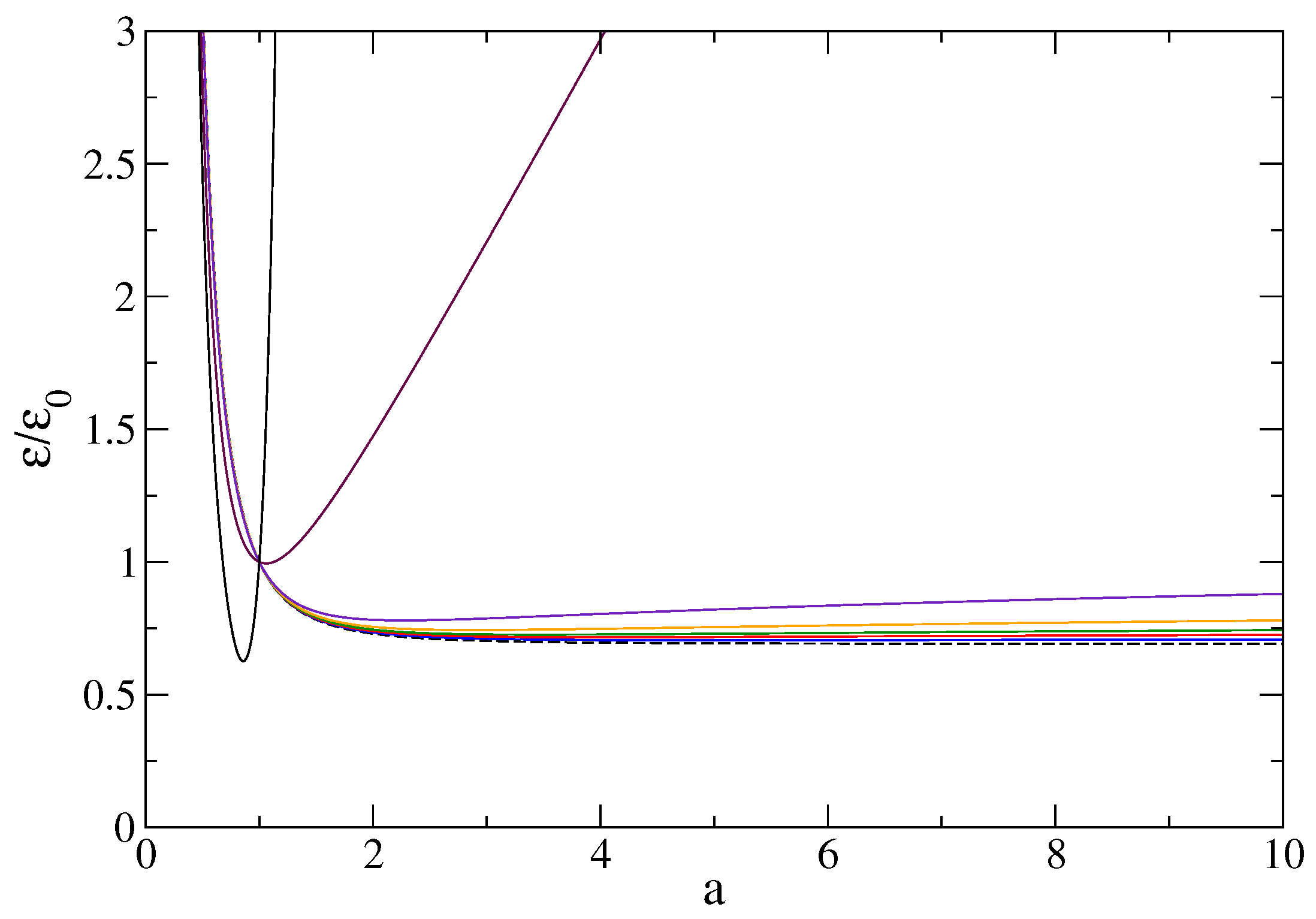
In the following we consider models with $A_i=A_n{\delta }_{i,n}$. The evolution of the energy density as a function of the scale factor [see Equation (39)] is plotted in Figure 1, where we have used the best-fit values of the parameters ${\Omega }_{m,0}=0.309$ and $B=3.53\times {10}^{-3}$ obtained from the $\Lambda$CDM model (they are consistent with the cosmological analysis of the original logotropic model [40,41]). The Universe starts at $a=0$ with an infinite energy density 5. The energy density $ϵ$ first decreases with the increase in the scale factor a, reaches a minimum, then increases with the scale factor characterizing a phantom Universe [48,49].

In the generalized logotropic model, the Friedmann Equation (26) takes the form

$$\begin{array}{c}\hfill H=\frac{\dot{a}}{a}=H_0\sqrt{\frac{{\Omega }_{m,0}}{a^3}+\frac{1-{\Omega }_{m,0}}{a^3}\frac{\Gamma \left(n+1,-1-\frac{1}{B}-3lna\right)}{\Gamma \left(n+1,-1-\frac{1}{B}\right)}}.\end{array}$$

(67)

The evolution of the scale factor as a function of the time is given by

$$\begin{array}{c}\hfill H_{0}t={\int }_0^a\frac{d{a}^{\prime }}{a^{\prime }\sqrt{\frac{{\Omega }_{m,0}}{a^{\prime 3}}+\frac{1-{\Omega }_{m,0}}{a^{\prime 3}}\frac{\Gamma \left(n+1,-1-\frac{1}{B}-3ln{a}^{\prime }\right)}{\Gamma \left(n+1,-1-\frac{1}{B}\right)}}}.\end{array}$$

(68)

The $\Lambda$CDM model is recovered from Equation (68) for $n=0$ or $B=0$. In that case, Equation (68) can be integrated analytically yielding

$$\begin{array}{c}\hfill a={\left(\frac{{\Omega }_{m,0}}{1-{\Omega }_{m,0}}\right)}^{1/3}{sinh}^{2/3}\left(\frac{3}{2}\sqrt{1-{\Omega }_{m,0}}{H}_{0}t\right),\end{array}$$

(69)

$$\begin{array}{c}\hfill \frac{ϵ}{{ϵ}_0}=\frac{1-{\Omega }_{m,0}}{{tanh}^2\left(\frac{3}{2}\sqrt{1-{\Omega }_{m,0}}{H}_{0}t\right)},\end{array}$$

(70)

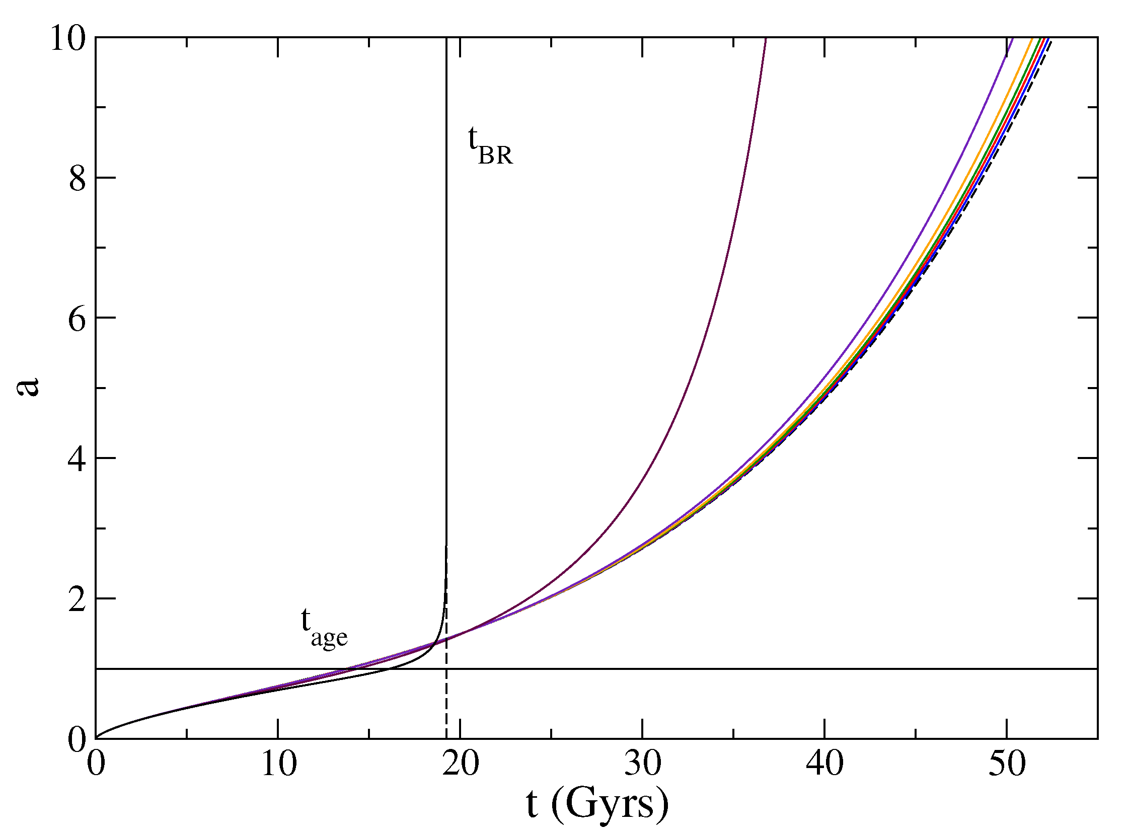
whereas for $B\ne 0$ it can only be integrated numerically. Figure 2 shows the behavior of the scale factor a as a function of t for $n=0,1,2,3,5,10,100,1000$. The age of the universe (corresponding to $a=1$) is given by

$$\begin{array}{c}\hfill t_{\mathrm{age}}=\frac{1}{H_0}{\int }_0^1\frac{d{a}^{\prime }}{a^{\prime }\sqrt{\frac{{\Omega }_{m,0}}{a^{\prime 3}}+\frac{1-{\Omega }_{m,0}}{a^{\prime 3}}\frac{\Gamma \left(n+1,-1-\frac{1}{B}-3ln{a}^{\prime }\right)}{\Gamma \left(n+1,-1-\frac{1}{B}\right)}}}\end{array}$$

(71)

with $H_0=2.195\times {10}^{-18}{\mathrm{s}}^{-1}$, i.e., $H_0^{-1}=14.4\mathrm{Gyrs}$. For the $\Lambda$CDM model ($n=0$) we recover the well-known result $t_{\mathrm{age}}=0.956H_0^{-1}=13.8\mathrm{Gyrs}$. A difference larger than $0.1\%$ (the typical error bar on the age of the universe) occurs in models with $n>3$ so these models should be rejected 6. For example, we obtain $t_{\mathrm{age}}=0.966H_0^{-1}=13.9\mathrm{Gyrs}$ for $n=20$, $t_{\mathrm{age}}=0.998H_0^{-1}=14.4\mathrm{Gyrs}$ for $n=100$, and $t_{\mathrm{age}}=1.12H_0^{-1}=16.1\mathrm{Gyrs}$ for $n=1000$.

The asymptotic behavior of the generalized logotropic model can be obtained analytically. For $a\to 0$, we have a matter-dominated Universe which corresponds to Einstein-deSitter (EdS) solution given by

$$\begin{array}{c}\hfill a\sim {\left(\frac{3}{2}\sqrt{{\Omega }_{m,0}}{H}_{0}t\right)}^{2/3},\end{array}$$

(72)

$$\begin{array}{c}\hfill \frac{ϵ}{{ϵ}_0}\sim \frac{4}{9H_0^2{t}^2}.\end{array}$$

(73)

For $a\to +\infty$, the energy density behaves as

$$\begin{array}{c}\hfill ϵ\sim 3^n\left|A_n\right|{(lna)}^n.\end{array}$$

(74)

In this asymptotic regime, the Friedmann equation can be written as

$$\begin{array}{c}\hfill \frac{\dot{a}}{a}=\sqrt{\frac{8\pi G}{3c^2}ϵ}\sim K_n{(lna)}^{n/2},\end{array}$$

(75)

where we define the constant $K_n$ as

$$\begin{array}{c}\hfill K_n=3^{n/2}{H}_0\sqrt{\frac{\left(1-{\Omega }_{m,0}\right)e^{1+1/B}}{\Gamma \left(n+1,-1-\frac{1}{B}\right)}}.\end{array}$$

(76)

The above equation can be integrated into

$$\begin{array}{c}\hfill K_{n}t\sim {\int }^a\frac{d{a}^{\prime }}{a^{\prime }{(ln{a}^{\prime })}^{n/2}}\sim {\int }^{lna}\frac{ds}{s^{n/2}},\end{array}$$

(77)

where we have made the change of variables $s=ln{a}^{\prime }$ to obtain the second equality. It is interesting to note that the asymptotic evolution of the scale factor as a function of time depends mainly on the value of the parameter n. We can distinguish three relevant types of evolution which correspond to $n<2,n=2$ and $n>2$.

(i) For $n<2$: this solution, which includes the original logotropic model [30,31,40], describes a super de Sitter evolution of the form

$$\begin{array}{c}\hfill a\propto \exp \left\{{\left[\frac{1}{2}(2-n)K_{n}t\right]}^{\frac{2}{2-n}}\right\},ϵ\propto t^{\frac{2n}{2-n}},\end{array}$$

(78)

where the scale factor grows super exponentially rapidly with cosmic time causing an algebraic divergence of the energy density. For $n=1$ we recover the original logotropic model where $a\sim e^{t^2}$ and $ϵ\sim t^2$ [30,31,40]. Since the scale factor and the energy density increase indefinitely with time, this is called Little Rip [50]. For $n=0$ we recover the $\Lambda$CDM model presenting an exponential (de Sitter) expansion $a\sim e^t$ and a constant energy density $ϵ\sim 1$.

(ii) For $n=2$: we obtain a double exponential evolution of the form

$$\begin{array}{c}\hfill a\propto \exp [\exp \left(K_{2}t\right)],ϵ\propto \exp \left(2K_{2}t\right),\end{array}$$

(79)

where the scale factor grows hyper exponentially rapidly with cosmic time causing an exponential divergence of the energy density (Little Rip).

(iii) For $n>2$: this case represents a situation in which the Universe ends up with a finite-time future singularity. One finds

$$\begin{array}{c}\hfill a\propto \exp \left\{{\left[\frac{1}{2}(n-2)K_n(t_s-t)\right]}^{-\frac{2}{n-2}}\right\},ϵ\propto {\left[\frac{1}{2}(n-2)K_n(t_s-t)\right]}^{-\frac{2n}{n-2}}.\end{array}$$

(80)

The singularity at $t=t_s$ corresponds to a Big Rip [49] characterized by the divergence of the scale factor and energy density in finite time. The big rip time (corresponding to $a\to +\infty$) is given by

$$\begin{array}{c}\hfill t_{\mathrm{BR}}=\frac{1}{H_0}{\int }_0^{+\infty }\frac{d{a}^{\prime }}{a^{\prime }\sqrt{\frac{{\Omega }_{m,0}}{a^{\prime 3}}+\frac{1-{\Omega }_{m,0}}{a^{\prime 3}}\frac{\Gamma \left(n+1,-1-\frac{1}{B}-3ln{a}^{\prime }\right)}{\Gamma \left(n+1,-1-\frac{1}{B}\right)}}}.\end{array}$$

(81)

For measured values of ${\Omega }_{m,0}$ and ${ϵ}_0$ (hence $H_0$), this is just a function of n. There is no other free (undetermined) parameter in our model. We obtain $t_{\mathrm{BR}}=3240\mathrm{Gyrs}$ for $n=3$, $t_{\mathrm{BR}}=1650\mathrm{Gyrs}$ for $n=4$, $t_{\mathrm{BR}}=422\mathrm{Gyrs}$ for $n=10$, $t_{\mathrm{BR}}=47.1\mathrm{Gyrs}$ for $n=100$, and $t_{\mathrm{BR}}=19.2\mathrm{Gyrs}$ for $n=1000$. However, we recall that the models with $n>3$ are excluded from the observations.

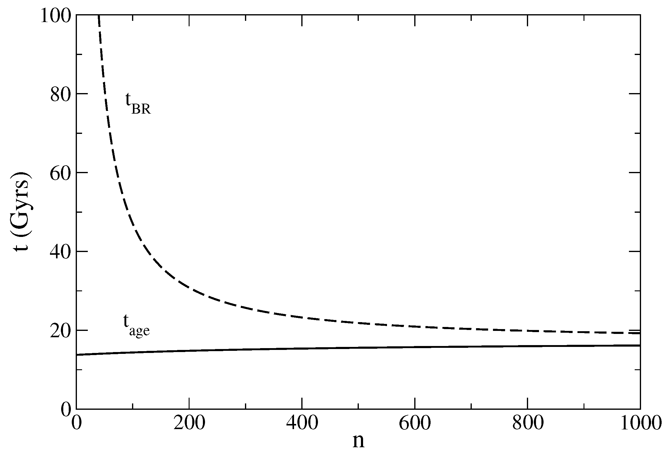
We note that the expansion of the Universe at late times is faster for higher n. In particular, the big rip time (when $n>2$) decreases with n. Still the age of the Universe (calculated at $a=1$) slightly increases with n. Therefore, for higher n, the Universe is older than for the $\Lambda$CDM model, and not younger. This counterintuitive behavior is illustrated in Figure 2. There is no paradox since it is only asymptotically (for $a\to +\infty$) that the expansion of the Universe is faster for higher n. For intermediate times (around $a\sim 1$), it is slower. We have plotted the age of the Universe and the big rip time as a function of n in Figure 3 to show their different evolutions.

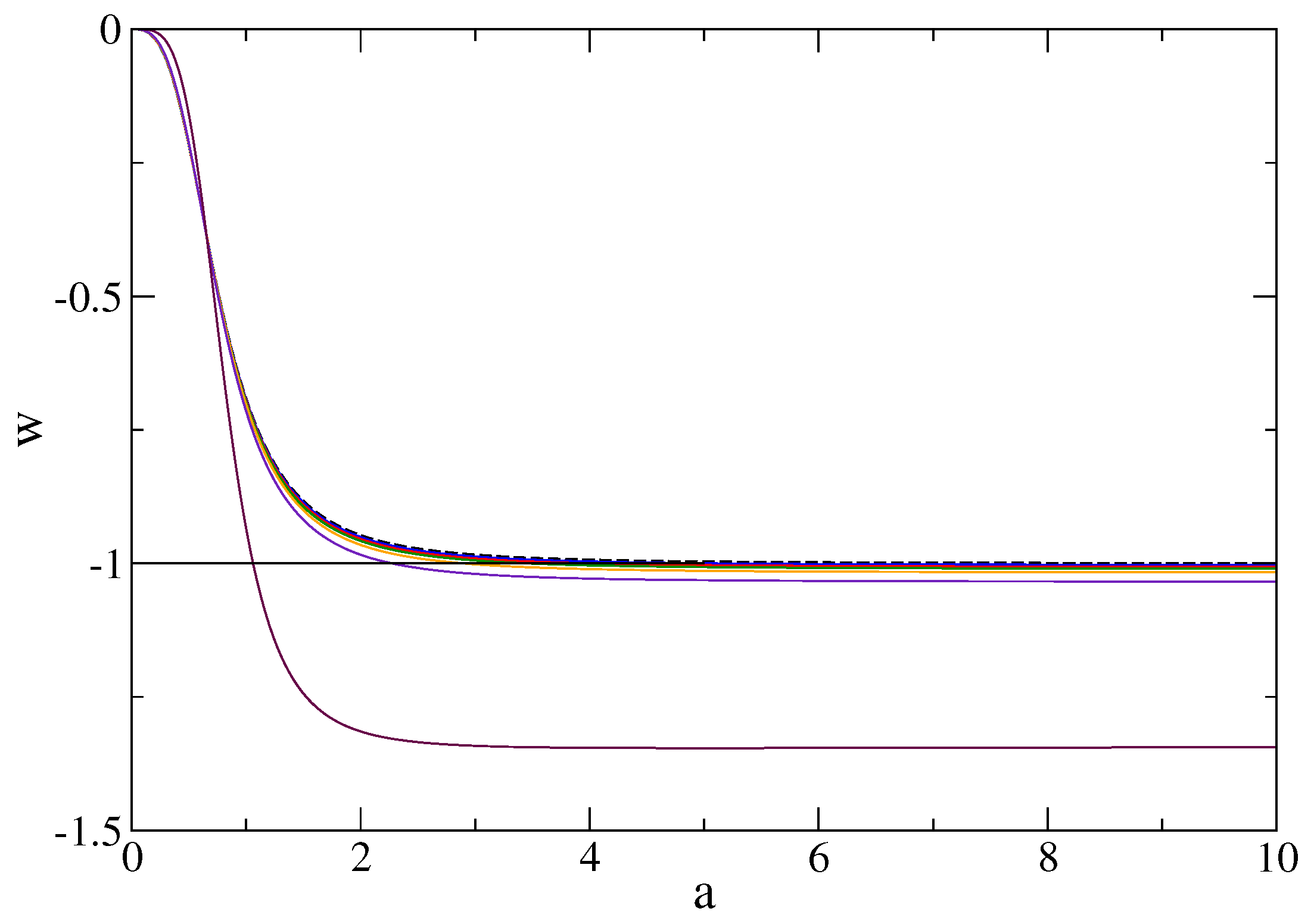
Using Equations (38) and (39), the EoS parameter $w=P/ϵ$ can be expressed in terms of the scale factor as

$$\begin{array}{c}\hfill w\left(a\right)=\frac{-\left(1-{\Omega }_{m,0}\right)e^{1+1/B}{a}^3{\left(-1-\frac{1}{B}-3lna\right)}^n}{{\Omega }_{m,0}\Gamma \left(n+1,-1-\frac{1}{B}\right)+\left(1-{\Omega }_{m,0}\right)\Gamma \left(n+1,-1-\frac{1}{B}-3lna\right)}.\end{array}$$

(82)

For $a=1$, we obtain

$$\begin{array}{c}\hfill w_0=-\frac{\left(1-{\Omega }_{m,0}\right)e^{1+1/B}{\left(-1-\frac{1}{B}\right)}^n}{\Gamma \left(n+1,-1-\frac{1}{B}\right)}.\end{array}$$

(83)

For the $\Lambda$CDM ($n=0$) we recover the well-known value $w_0=-\left(1-{\Omega }_{m,0}\right)=-0.691$. We obtain $w_0=-0.693$ for $n=1$, $w_0=-0.696$ for $n=2$, $w_0=-0.698$ for $n=3$, $w_0=-0.701$ for $n=4$, $w_0=-0.715$ for $n=10$, $w_0=-0.935$ for $n=100$, and $w_0=-3.12$ for $n=1000$. For $n>3$ we are out of the error bars (typically $1\%$ for the value of $w_0$) so these models should be rejected. The behavior of the EoS parameter $w\left(a\right)$ as a function of the scale factor a is plotted in Figure 4. The GLDF behaves as a superposition of two non-interacting fluids (i.e., DM and DE) whose total pressure and total energy density are given by the sums

$$\begin{array}{c}\hfill P=P_m+P_{de},ϵ={ϵ}_m+{ϵ}_{de}.\end{array}$$

(84)

Their EoS parameters are

$$\begin{array}{c}\hfill w_m=\frac{P_m}{{ϵ}_m}=0,w_{de}=\frac{P_{de}}{{ϵ}_{de}}=-\frac{e^{1+1/B}{a}^3{\left(-1-\frac{1}{B}-3lna\right)}^n}{\Gamma \left(n+1,-1-\frac{1}{B}-3lna\right)}.\end{array}$$

(85)

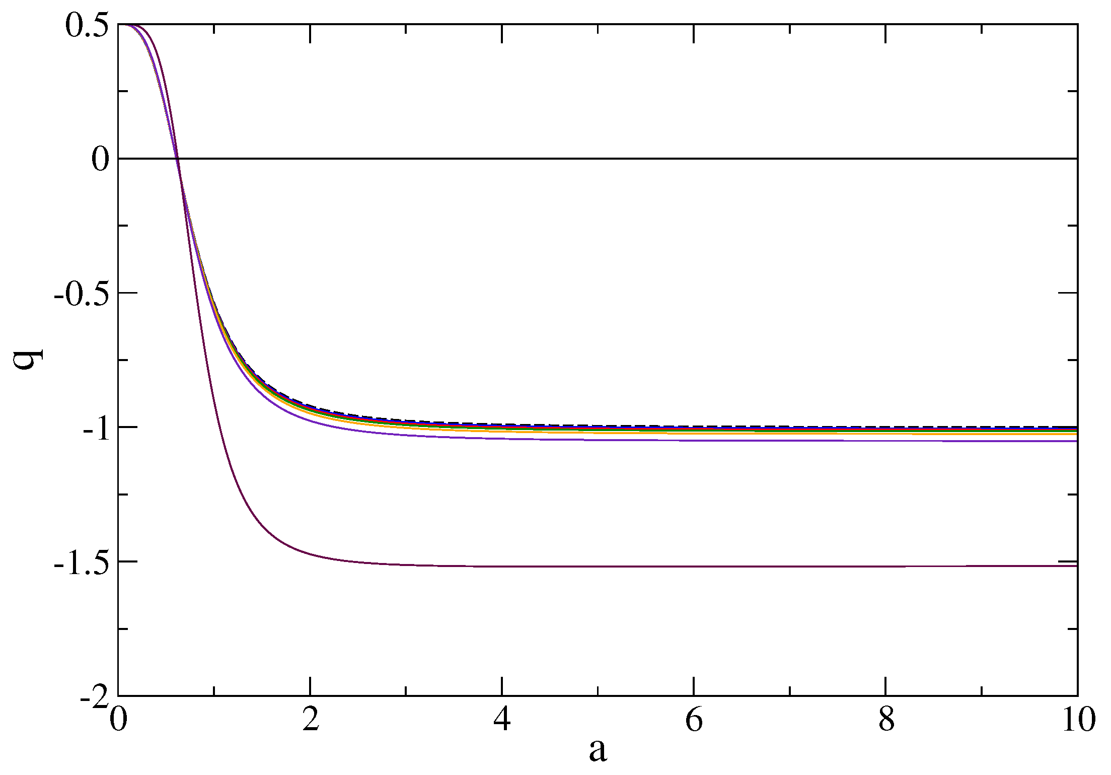
In a flat Universe, the deceleration parameter $q=-\ddot{a}a/{\dot{a}}^2=-\dot{H}/H^2-1$ is related to the EoS parameter by

$$\begin{array}{c}\hfill q=\frac{1+3w}{2}.\end{array}$$

(86)

The Universe is undergoing a decelerating expansion if $q>0$ (i.e., $w>-1/3$) and an accelerating expansion if $q<0$ (i.e., $w<-1/3$). In Figure 5, we show the behavior of $q\left(a\right)$ as a function of the scale factor for different values of n.

From Equation (39), the transition scale factor $a_t$, corresponding to ${ϵ}_m={ϵ}_{de}$, is obtained by solving the transcendental equation

$$\begin{array}{c}\hfill \Gamma \left(n+1,-1-\frac{1}{B}-3ln{a}_t\right)=\frac{{\Omega }_{m,0}}{1-{\Omega }_{m,0}}\Gamma \left(n+1,-1-\frac{1}{B}\right).\end{array}$$

(87)

Another parameter to study is the squared speed of sound $c_s^2$ which is a key ingredient to investigate the stability of any model. In particular, the sign of $c_s^2$ plays a crucial role in determining classical stability. It is defined by

$$\begin{array}{c}\hfill c_s^2=\frac{dP}{dϵ}{c}^2=\frac{dP/d{\rho }_m}{dϵ/d{\rho }_m}{c}^2.\end{array}$$

(88)

Differentiating Equations (1) and (13) with $A_i=A_n{\delta }_{i,n}$, we obtain

$$\begin{array}{c}\hfill \frac{c_s^2}{c^2}=\frac{n{ln}^{n-1}\left(\frac{{\rho }_m}{{\rho }_P}\right)}{\frac{{\rho }_m{c}^2}{A_n}-n\frac{{\rho }_m}{{\rho }_P}\Gamma \left[n,ln\left(\frac{{\rho }_m}{{\rho }_P}\right)\right]}.\end{array}$$

(89)

To obtain this expression, we have used the identities

$$\begin{array}{c}\hfill \Gamma (n+1,x)=n\Gamma (n,x)+x^n{e}^{-x}\end{array}$$

(90)

and

$$\begin{array}{c}\hfill \frac{\partial \Gamma }{\partial x}(n+1,x)=-x^n{e}^{-x}.\end{array}$$

(91)

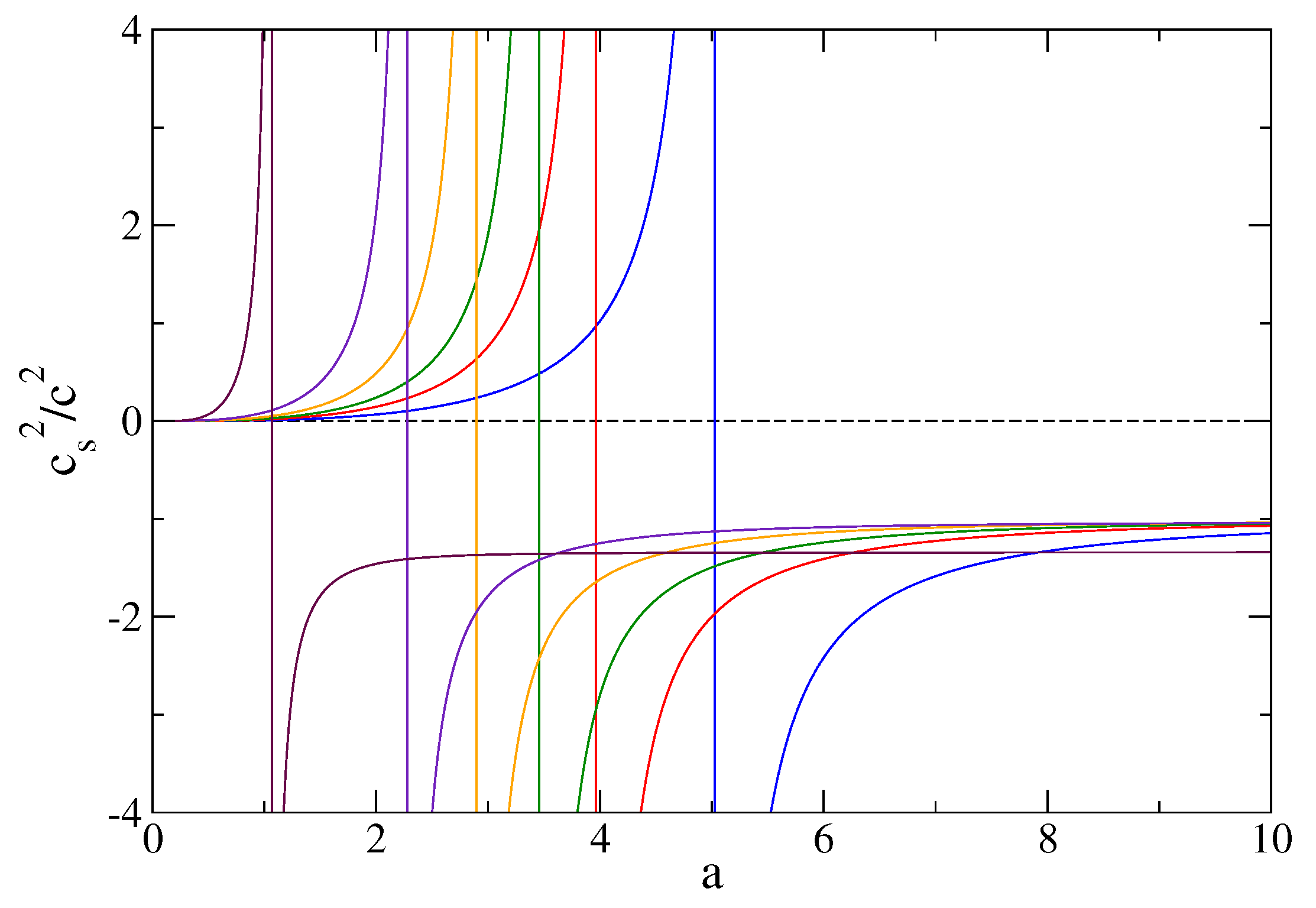
In Figure 6, we plot the squared speed of sound $c_s^2/c^2$ as a function of the scale factor for different values of n. The causality and classical stability conditions are satisfied if the speed of sound varies in the range $0\le c_s^2/c^2\le 1$. One sees from Figure 6 that, in fact, there are regions where the causality and classical stability conditions are satisfied but the extent of these regions decreases as n increases 7.

6. Conclusions

In this work, we have proposed a new class of cosmological unified dark sector models “Generalized Logotropic Models”. These models are a generalization of the logotropic model [30] by considering the pressure P as a sum of higher logarithmic terms of the rest-mass density ${\rho }_m$. The pressure can naturally take negative values in these cosmological models. In this scenario, the Universe is filled with a single fluid without the need for a cosmological constant. Our generalized model depends on a set of free parameters $A_i$ with $i=1,2,\cdots ,N$. In particular, we have considered a special class of generalized logotropic models where $A_i=A_n{\delta }_{in}$, which depends on two free parameters $A_n$ and n. The usual logotropic model [30] corresponds to $n=1$ and $A_1$. We have also presented the model with $N=2$, which contains the first two terms $A_1$ and $A_2$ of the series. We have highlighted the most relevant properties of these generalized logotropic models. To fix bounds on the free parameters of our models, we employed the best fit of the parameters ${\Omega }_{m,0}$ and B obtained from the cosmological analysis carried on the original logotropic model (i.e., $n=1$) [40]. After fixing the free parameters, we investigated the cosmological behavior of the generalized logotropic models by focusing on the evolution of the DE density, scale factor, EoS parameter, deceleration parameter and squared speed of sound. We showed the asymptotic behavior of these models and noticed three distinct ways of evolution depending on the value of n. In all the analyzed cases, we established that generalized logotropic models lead to realistic cosmological models in which the dark sector is represented by a unique fluid. The deviation of the generalized models from the standard $\Lambda$CDM model depends on the value of the parameter n. At later times, higher values of n lead to higher deviations from $\Lambda$CDM. This implies that the generalized logotropic models can be used as realistic background cosmological models to describe our Universe with a free parameter n. We estimated that only models with $n\le 3$ are consistent with the observations. To find out the most suitable values of n, it will be necessary to perform a fitting procedure by using, for instance, the Monte Carlo method and a detailed comparison with cosmological data such as SN, BAO, and CMB surveys. We expect to perform this analysis in future works.

A further interesting generalization of the logotropic model is to consider a single fluid described by the EoS

$$\begin{array}{c}\hfill P=A{ln}^{\alpha }\left(\frac{{\rho }_m}{{\rho }_P}\right),\end{array}$$

(92)

where A is a real number given by

$$\begin{array}{c}\hfill A=-\frac{\left(1-{\Omega }_{m,0}\right){ϵ}_0{e}^{1+1/B}}{\Gamma \left(\alpha +1,-1-\frac{1}{B}\right)},\end{array}$$

(93)

and $\alpha$ is a real positive parameter that can be constrained by the cosmological data. There are two ways to recover the $\Lambda$CDM, either by taking $\alpha =0$ or $B=0$ which makes the model rich and particularly more appealing in describing DE especially for $0<\alpha <1$. Such a model interpolates between the $\Lambda$CDM for values of $\alpha$ close to zero and to the usual logotropic model for values of $\alpha$ close to one.

In summary, single fluids with generalized logotropic EoS may have interesting cosmological features and, thus, they represent a good candidate to describe the DE sector. The investigation and analysis of these models will be carried out in detail in future works.

Finally, we would like to mention that the logotropic model and the generalization presented in this work are not free of intrinsic problems, as all the cosmological models known in the literature. In fact, the speed of sound in logotropic models has the unpleasant property of increasing with the scale factor, leading, like for the Chaplygin gas model, to oscillations in the mass power-spectrum that are not detected in observations at the cosmological level [51]. However, there are several possibilities to solve this problem by considering additional effects such as non-linear and non-adiabatic perturbations, or higher order derivatives in K-essence Lagrangians associated with braneworld models, among others (see the discussion in Section XVI.G of [46]). These modifications could solve the problems in the theory of perturbations for structure formation (e.g., by reducing the speed of sound) without affecting the evolution of the cosmological background. In any case, UDM models constitute a subject of intensive research as possible alternative scenarios to the popular and generally accepted $\Lambda$CDM model. Our paper provides a class of models exhibiting a transition between a normal behavior and a phantom behavior governed by a single equation of state. In addition, depending on the value of the parameter n, we can have different types of late evolution: no singularity ($n=0$), little rip ($n\le 2$), big rip ($n>2$). It is very interesting to note that all these models are consistent with the $\Lambda$CDM model up to the present time but will differ in the future. Therefore, it is possible to construct models that agree with the observations but that deviate from each other at late times. A virtue of our model is to show that it is very difficult to predict the future evolution of the Universe based on present observations.

References

- Riess, A.G.; Filippenko, A.V.; Challis, P.; Clocchiatti, A.; Diercks, A.; Garnavich, P.M.; Gilliland, R.L.; Hogan, C.J.; Jha, S.; Tonry, J. Observational evidence from supernovae for an accelerating universe and a cosmological constant. Astron. J. 1998, 116, 1009. [Google Scholar] [CrossRef]
- Perlmutter, S.; Aldering, G.; Goldhaber, G.; Knop, R.A.; Nugent, P.; Castro, P.G.; Deustua, S.; Fabbro, S.; Goobar, A.; Groom, D.E.; et al. Supernova Cosmology Project. Measurements of Ω and Λ from 42 high-redshift supernovae. Astrophys. J. 1999, 517, 565. [Google Scholar] [CrossRef]
- Spergel, D.N.; Verde, L.; Peiris, H.V.; Komatsu, E.; Nolta, M.R.; Bennett, C.L.; Halpern, M.; Hinshaw, G.; Jarosik, N.; Wright, E.L.; et al. First-year Wilkinson Microwave Anisotropy Probe (WMAP)* observations: Determination of cosmological parameters. Astrophys. J. Suppl. Ser. 2003, 148, 175. [Google Scholar] [CrossRef]
- Tegmark, M.; Strauss, M.A.; Blanton, M.R.; Abazajian, K.; Dodelson, S.; Sandvik, H.; York, D.G. Cosmological parameters from SDSS and WMAP. Phys. Rev. D 2004, 69, 103501. [Google Scholar] [CrossRef]
- Ade, P.A.R.; Aghanim, N.; Armitage-Caplan, C.; Arnaud, M.; Ashdown, M.; Atrio-Barandela, F.; Aumont, J.; Baccigalupi, C.; Banday, A.J.; Meinhold, P.R.; et al. Planck 2013 results. XVI. Cosmological parameters. Astron. Astrophys. 2014, 571, A16. [Google Scholar]
- Sahni, V.; Starobinsky, A.A. The case for a positive cosmological Λ-term. Int. J. Modern Phys. D 2000, 9, 373–443. [Google Scholar] [CrossRef]
- Amendola, L.; Kunz, M.; Motta, M.; Saltas, I.D.; Sawicki, I. Observables and unobservables in dark energy cosmologies. Phys. Rev. D 2013, 87, 023501. [Google Scholar] [CrossRef]
- Weinberg, S. The cosmological constant problem. Rev. Mod. Phys. 1989, 61, 1. [Google Scholar] [CrossRef]
- Padmanabhan, T. Cosmological Constant—The Weight of the Vacuum. Phys. Rep. 2003, 380, 235. [Google Scholar] [CrossRef]
- Steinhardt, P. Critical Problems in Physics; Fitch, V.L., Marlow, D.R., Eds.; Princeton University Press: Princeton, NJ, USA, 1997. [Google Scholar]
- Zlatev, I.; Wang, L.; Steinhardt, P.J. Quintessence, cosmic coincidence, and the cosmological constant. Phys. Rev. Lett. 1999, 82, 896. [Google Scholar] [CrossRef]
- Moore, B.; Quinn, T.; Governato, F.; Stadel, J.; Lake, G. Cold collapse and the core catastrophe. Mon. Not. R. Astron. Soc. 1999, 310, 11471152. [Google Scholar] [CrossRef] [Green Version]
- Kauffmann, G.; White, S.D.M.; Guiderdoni, B. The formation and evolution of galaxies within merging dark matter haloes. Mon. Not. R. Astron. Soc. 1993, 264, 201–218. [Google Scholar] [CrossRef]
- Klypin, A.; Kravtsov, A.V.; Valenzuela, O. Where are the missing galactic satellites? Astrophys. J. 1999, 522, 82. [Google Scholar] [CrossRef]
- Kamionkowski, M.; Liddle, A.R. The dearth of halo dwarf galaxies: Is there power on short scales? Phys. Rev. Lett. 2000, 84, 4525. [Google Scholar] [CrossRef]
- Boylan-Kolchin, M.; Bullock, J.S.; Kaplinghat, M. Too big to fail? The puzzling darkness of massive Milky Way subhaloes. Mon. Not. R. Astron. Soc. Lett. 2011, 415, L40–L44. [Google Scholar] [CrossRef]
- Bullock, J.S.; Boylan-Kolchin, M. Small-Scale Challenges to the Λ CDM Paradigm. Ann. Rev. Astron. Astrophys. 2017, 55, 343. [Google Scholar] [CrossRef]
- Kamenshchik, A.; Moschella, U.; Pasquier, V. An alternative to quintessence. Phys. Lett. B 2001, 511, 265–268. [Google Scholar] [CrossRef]
- Benaoum, H.B. Accelerated Universe from Modified Chaplygin Gas and Tachyonic Fluid. Universe 2022, 8, 340. [Google Scholar] [CrossRef]
- Bento, M.C.; Bertolami, O.; Sen, A.A. Generalized Chaplygin gas, accelerated expansion, and dark-energy-matter unification. Phys. Rev. D 2002, 66, 043507. [Google Scholar] [CrossRef]
- Gorini, V.; Kamenshchik, A.; Moschella, U. Can the Chaplygin gas be a plausible model for dark energy? Phys. Rev. D 2003, 67, 063509. [Google Scholar] [CrossRef]
- Bento, M.C.; Bertolami, O.; Sen, A.A. Revival of the unified dark energy–dark matter model? Phys. Rev. D 2004, 70, 083519. [Google Scholar] [CrossRef] [Green Version]
- Debnath, U.; Banerjee, A.; Chakraborty, S. Role of modified Chaplygin gas in accelerated universe. Class. Quantum Grav. 2004, 21, 5609. [Google Scholar] [CrossRef]
- Benaoum, H.B. Modified Chaplygin Gas Cosmology. Adv. High Energy Phys. 2012, 2012, 357802. [Google Scholar] [CrossRef]
- Benaoum, H.B. Modified Chaplygin gas cosmology with bulk viscosity. Int. J. Mod. Phys. D 2014, 23, 1450082. [Google Scholar] [CrossRef]
- Chavanis, P.H. Models of universe with a polytropic equation of state: I. The early universe. Eur. Phys. J. Plus 2014, 129, 38. [Google Scholar] [CrossRef]
- Chavanis, P.H. Models of universe with a polytropic equation of state: II. The late universe. Eur. Phys. J. Plus 2014, 129, 222. [Google Scholar] [CrossRef]
- Chavanis, P.H. Models of universe with a polytropic equation of state: III. The phantom universe. arXiv 2012, arXiv:1208.1185. [Google Scholar]
- Chavanis, P.H. A cosmological model describing the early inflation, the intermediate decelerating expansion, and the late accelerating expansion of the universe by a quadratic equation of state. Universe 2015, 1, 357–411. [Google Scholar] [CrossRef]
- Chavanis, P.H. Is the Universe logotropic? Eur. Phys. J. Plus 2015, 130, 130. [Google Scholar] [CrossRef]
- Chavanis, P.H. The Logotropic Dark Fluid as a unification of dark matter and dark energy. Phys. Lett. B 2016, 758, 59–66. [Google Scholar] [CrossRef]
- Ferreira, V.M.C.; Avelino, P.P. New limit on logotropic unified dark energy models. Phys. Lett. B 2017, 770, 213–216. [Google Scholar] [CrossRef]
- Odintsov, S.D.; Oikonomou, V.K.; Timoshkin, A.V.; Saridakis, E.N.; Myrzakulov, R. Cosmological fluids with logarithmic equation of state. Ann. Phys. 2018, 398, 238. [Google Scholar] [CrossRef] [Green Version]
- Capozziello, S.; D’Agostino, R.; Luongo, O. Cosmic acceleration from a single fluid description. Phys. Dark Univ. 2018, 20, 1. [Google Scholar] [CrossRef]
- Chavanis, P.H. New predictions from the logotropic model. Phys. Dark Univ. 2019, 24, 100271. [Google Scholar] [CrossRef]
- Benaoum, H.B.; Luongo, O.; Quevedo, H. Extensions of modified Chaplygin gas from Geometrothermodynamics. Eur. Phys. J. C 2019, 79, 577. [Google Scholar] [CrossRef]
- Boshkayev, K.; D’Agostino, R.; Luongo, O. Extended logotropic fluids as unified dark energy models. Eur. Phys. J. C 2019, 79, 332. [Google Scholar] [CrossRef]
- Capozziello, S.; D’Agostino, R.; Giambò, R.; Luongo, O. Effective field description of the Anton-Schmidt cosmic fluid. Phys. Rev. D 2019, 99, 023532. [Google Scholar] [CrossRef]
- Li, H.; Yang, W.; Gai, L. Astronomical bounds on the modified Chaplygin gas as a unified dark fluid model. Astron. Astrophys. 2019, 623, A28. [Google Scholar] [CrossRef]
- Chavanis, P.H.; Kumar, S. Comparison between the Logotropic and ΛCDM models at the cosmological scale. J. Cosmol. Astropart. Phys. 2017, 1705, 018. [Google Scholar] [CrossRef]
- Mamon, A.A.; Saha, S. The logotropic dark fluid: Observational and thermodynamic constraints. Int. J. Mod. Phys. D 2020, 29, 2050097. [Google Scholar] [CrossRef]
- Boshkayev, K.; Konysbayev, T.; Luongo, O.; Muccino, M.; Pace, F. Testing generalized logotropic models with cosmic growth. Phys. Rev. D 2021, 104, 023520. [Google Scholar] [CrossRef]
- Donato, F.; Gentile, G.; Salucci, P.; Frigerio Martins, C.; Wilkinson, M.I.; Gilmore, G.; Grebel, E.K.; Koch, K.; Wyse, R. A constant dark matter halo surface density in galaxies. Mon. Not. R. Astron. Soc. 2009, 397, 1169–1176. [Google Scholar] [CrossRef] [Green Version]
- Chavanis, P.H. Predictions from the logotropic model: The universal surface density of dark matter halos and the present proportions of dark matter and dark energy. Phys. Dark Univ. 2022, 37, 101098. [Google Scholar] [CrossRef]
- Chandrasekhar, S. An Introduction to the Theory of Stellar Structure; University of Chicago Press: Chicago, IL, USA, 1939. [Google Scholar]
- Chavanis, P.H. A new logotropic model based on a complex scalar field with a logarithmic potential. arXiv 2022, arXiv:2201.05908. [Google Scholar]
- Weinberg, S. Gravitation and Cosmology; John Wiley: New York, NY, USA, 2020. [Google Scholar]
- Caldwell, R.R. A phantom menace? Cosmological consequences of a dark energy component with super-negative equation of state. Phys. Lett. B 2002, 545, 23. [Google Scholar] [CrossRef]
- Caldwell, R.R.; Kamionkowski, M.; Weiberg, N.N. Phantom energy: Dark energy with w<−1 causes a cosmic doomsday. Phys. Rev. Lett. 2003, 91, 071301. [Google Scholar]
- Frampton, P.H.; Ludwick, K.J.; Scherrer, R.J. The little rip. Phys. Rev. D 2011, 84, 063003. [Google Scholar] [CrossRef]
- Sandvik, H.; Tegmark, M.; Zaldarriaga, M.; Waga, I. The end of unified dark matter? Phys. Rev. D 2004, 69, 123524. [Google Scholar] [CrossRef]
Figure 1.
Normalized energy density as a function of the scale factor a for , and various values of n: (dashed black, CDM model), (blue, original logotropic model), (red), (green), (orange), (indigo), (maroon), (black).
Figure 2.
Scale factor a as a function of the cosmic time t for , and . This figure shows the big rip time (for ) at which the scale factor becomes infinite.
Figure 3.
Age of the Universe and big rip time as a function of n.
Figure 4.
EoS parameter w as a function the scale factor a for , and .
Figure 5.
Deceleration parameter q as a function of the scale factor a for , and .
Figure 6.
Normalized squared speed of sound as a function of the scale factor a for , and . It diverges and becomes negative when the Universe becomes phantom.
Publisher’s Note: MDPI stays neutral with regard to jurisdictional claims in published maps and institutional affiliations. |
© 2022 by the authors. Licensee MDPI, Basel, Switzerland. This article is an open access article distributed under the terms and conditions of the Creative Commons Attribution (CC BY) license (https://creativecommons.org/licenses/by/4.0/).
Share and Cite
MDPI and ACS Style
Benaoum, H.; Chavanis, P.-H.; Quevedo, H. Generalized Logotropic Models and Their Cosmological Constraints. Universe 2022, 8, 468. https://doi.org/10.3390/universe8090468
AMA Style
Benaoum H, Chavanis P-H, Quevedo H. Generalized Logotropic Models and Their Cosmological Constraints. Universe. 2022; 8(9):468. https://doi.org/10.3390/universe8090468
Chicago/Turabian StyleBenaoum, Hachemi, Pierre-Henri Chavanis, and Hernando Quevedo. 2022. "Generalized Logotropic Models and Their Cosmological Constraints" Universe 8, no. 9: 468. https://doi.org/10.3390/universe8090468
Note that from the first issue of 2016, this journal uses article numbers instead of page numbers. See further details here.