
Splashback Radius in a Spherical Collapse Model
1
Dipartimento di Fisica e Astronomia, University of Catania, Viale Andrea Doria 6, 95125 Catania, Italy
2
Institute of Astronomy, Russian Academy of Sciences, Pyatnitskaya str., 48, 119017 Moscow, Russia
3
Institute of Theoretical Physics, School of Physical Science and Technology, Lanzhou University, No. 222, South Tianshui Road, Lanzhou 730000, China
4
Instituto de Astrofísica e Ciências do Espaço, Faculdade de Ciências, Universidade de Lisboa, Ed. C8, Campo Grande, 1769-016 Lisboa, Portugal
5
Lanzhou Center for Theoretical Physics, Key Laboratory of Theoretical Physics of Gansu Province, Lanzhou University, Lanzhou 730000, China
*
Author to whom correspondence should be addressed.
Universe 2022, 8(9), 462; https://doi.org/10.3390/universe8090462
Submission received: 5 August 2022
/
Revised: 29 August 2022
/
Accepted: 2 September 2022
/
Published: 6 September 2022
(This article belongs to the Special Issue Modified Gravity and Dark Matter at the Scale of Galaxies)
Abstract
:It was shown several years ago that dark matter halo outskirts are characterized by very steep density profiles in a very small radial range. This feature has been interpreted as a pile-up of different particle orbits at a similar location, namely, splashback material at half an orbit after collapse. Adhikari et al. (2014) obtained the location of the splashback radius through a very simple model by calculating a dark matter shell trajectory in the secondary infall model while it crosses a growing NFW profile-shaped dark matter halo. Because they imposed a halo profile instead of calculating it from the trajectories of the shells of dark matter, they were not able to find the dark matter profile around the splashback radius. In the present paper, we use an improved spherical infall model taking into account shell crossing as well as several physical effects such as ordered and random angular momentum, dynamical friction, adiabatic contraction, etc. This allows us to determine the density profile from the inner to the outer region and to study the behavior of the outer density profile. We compare the density profiles and their logarithmic slope of with the simulation results of Diemer and Kravtsov (2014), finding a good agreement between the prediction of the model and the simulations.
PACS:
98.52.Wz; 98.65.Cw1. Introduction
The problem of determining the structure of dark matter haloes is an old one, and has been studied from analytical, numerical, and observational points of view. The first efforts were based on analytical models, in particular, on the spherical collapse model. The first trials to study the formation of virialized structure go back to the seminal paper by [1], after which several authors investigated the consequences of secondary infall and accretion onto proto-structures, studying in particular the structure of the density profiles. In [2], the authors studied the self-similar collapse of scale-free perturbations, determining important processes in the halo profiles. Several other papers have improved on these results, e.g., [3,4,5,6,7,8,9]. These and other studies improved the secondary infall model (SIM) by taking into account the effects of ordered and random angular momentum, adiabatic contraction of dark matter (DM) produced by baryons [10,11,12], the effects of dynamical friction, and many more effects. Further developments were obtained by means of DM-only N-body simulations with the determination of the Navarro–Frenk–White profile [13,14], the Einasto profile [15,16], and hydrodynamic simulations [17,18]. Much of the past work focused on the inner structure of haloes and was driven by efforts to understand and solve the cusp–core problem, that is, the discrepancy between the steep slopes predicted by DM-only simulations and the flat-cored profiles observed in low surface brightness (LSB) and dwarf galaxies. In the last several years, authors (e.g., [19]) have begun to study the outer part of haloes, finding that the outer profiles are inconsistent with typical fits such as the NFW and Einasto profiles. Findings include that the outer density profiles are characterized over a narrow range of radii by very steep logarithmic slopes of . According to [19], the observed local steepening is due to a caustic related to the splashback of material accreted by the halo. The presence of caustics is due to the pile-up of different particle orbits at a similar location. The splashback radius corresponds to the outermost caustic associated with the first apoapse after collapse. As shown in [20], the splashback location is provided by the relation . Caustics are not a rare phenomenon; they are present in the [2] similarity solutions, in 3D similarity solutions of the collapse of triaxial peaks [21], and in real galaxies, where they appear as radial shells [22]. However, detecting density enhancement related to caustics in N-body simulations of dark haloes is not easy. This is mainly due to the presence of small-scale structures that can smear out caustics [23,24]. As material accumulates, a steepening in the outer profile is observed at the splashback radius. A few years ago, [20] estimated the location of the splashback radius using a very simplified secondary collapse model to obtain the secondary infall trajectory of DM shells by means of a growing DM halo with an NFW profile. In their calculation, a shape of the halo profile was imposed instead of being computed from the trajectories of the DM shells. As a consequence, in their calculation they were not able to obtain the full shape of the DM profile around the splashback radius. In the following, we introduce a much more complex spherical collapse model which allows us to simultaneously calculate the trajectories and the DM halo profile.
The paper is organized as follows. In Section 2, we discuss the model used to determine the density profile and which allows us to determine of the features of the outer profile. In Section 4 we discuss the results following from the model and compare them with the results of [19]’s simulations. Section 5 is devoted to further discussion.
2. Model
In this section, we discuss the model that allows us to determine the density profile. It was first introduced in [8], followed by several applications: to density profiles universality studies [25,26], to galaxies [27,28] and clusters [28,29] density profiles, and to galaxies’ inner surface-density distributions [30].
The semi-analytical model (SAM) used in this work encompasses several upgrades on the SIM (e.g., [1,3,4,5,6,7,9,31,32]). In contrast to the anterior avatars of the SIM, it comprises non-radial collapse effects from random angular momentum (RAM [5,6,33,34,35,36,37,38,39,40])1, ordered, tidal angular momentum [41,42], and the impact of dynamical friction (e.g., [8,43,44,45]) and of baryonically-induced DM adiabatic contraction [10,11,12].
This SAM evolves perturbations from their linear expansion with the Hubble flow to turn-around before collapsing, with adiabatic central potential variations including “shell-crossing” [2,46].
Spherical SIMs2 in the filiation from [1] describe a bound mass shell expansion from a comoving initial radius to its maximum (turn-around or apapsis) radius ,
with the linearly grown mean overdensity inside the shell extrapolated at current epoch and with obtained as in Appendix B of [8], results from
This generalisation represents the core of the SIM, for which a Lagrangian shell’s time averaged radius remains proportional to its initial radius. Using Equation (3), the final radius x can be written as proportional to the turn around radius, :
with the scaling fitted by [48]:
Beyond turnaround, shell crossing effects are bypassed with the Virial theorem, yielding a collapse factor , resulting in the final density profile through mass conservation:
This produces the power-law density profile from [3] from the shell’s initial density approximation
and the linear expansion of Equation (3), reading
However, the Virial theorem relies on energy conservation, and oscillations of collapsing shells through their inner shells break up the energy integral of motion and vary the value of f.
This modifies the SIM dynamics, which assume a “gentle” collapse, as follows: with the conjecture of adiabatic variation of the central potential [2,46], shells near the centre oscillate many times without significant changes in potential. In other words, inner shells’ orbital period can be neglected compared with outer shells’ collapse time [49]. In this case, the inner shells admit the radial action , with the radial velocity as adiabatic invariant. The collapse of outer shells slowly changes the potential, shrinking the inner shells via the radial action invariant.
The mass inside a shell with initial radius at its apocenter (apapsis radius) can be decomposed in the sum of its inner shells masses, i.e., with apocenters inside , the permanent component ; with the contribution from its temporarily crossing outer shells masses, the additional mass is . Mass conservation yields the first component,
with initial time constant density of the homogeneous Universe. From Equation (6), the distribution of mass and the system radius R, its outer shell apapsis, together with the probability to find the shell with apapsis x inside the radius , follows the additional component
with the resulting total mass reading
The ratio of the time spent below to the outer shell’s x oscillation period allows to be computed from the outer shell’s pericenter and , its radial velocity at radius , as follows:
The outer shell’s radial velocity derives from integrating its equation of motion, including the tidal torque-generated ordered specific angular momentum3 , the random angular momentum (see [8,33] and follow ups), the gravitational potential acceleration , (the cosmological constant), and the dynamical friction coefficient :
Computations of and the angular momenta are explained in ([8], Appendices C and D). In the restriction where , Equation (14) integrates into the square of velocity:
where the shell’s specific binding energy results from the turnaround value at at in Equation (15).
With the above computations complete, following [2,46] we obtain the shell’s collapse factor, which starts at radius and reaches apapsis
from Equations (6) and (4), the corresponding density profile at Virialisation is
The calculations above allow us to evaluate the variations from energy integral break up, confirmed from N-body simulations, finding its relation to the initial density perturbation profile and its increase with initial radius. The case and recovers a radial collapse [50]. The computation from Equation (17) of f via integration of Equation (11) can proceed numerically after variable change to express them in terms of initial radius [38,50]. Such variable change turns Equation (11) into
with ,
taking , and the initial shell’s pericenter . The upper bound of Equation (19)’s integration corresponds to the presently collapsed sphere’s initial radius. A similar variable change in Equation (16) leads to the determination of the radial velocity v for a shell characterised with apapsis at radius through
with the shifted gravitational potential from the initial mass profile reading
In summary (see [50], Section 4), the equation of motions of a shell (21), given the angular momentum distribution, dynamical friction coefficient, and initial conditions, integrates to compute , the probability from Equation (20), which then yields the transient part of the gravitating mass acting on the shell from Equation (19) and the collapse factor f from Equation (17) to obtain the final density profile through Equation (18) (as in [5], Section 2.1). Our model’s ordered angular momentum formation follows ([8], Appendix C1), its random angular momentum computation agrees with ([8], Appendix C2), its dynamical friction coefficient and the baryon dissipative collapse are described in ([8], Appendix D), the baryon’s adiabatic contraction is the object of ([8], Appendix E), and [Appendix B [8] describes initial condition generation. More explicitly, the model’s “ordered angular momentum” h derives from the tidal torque theory (TTT) [41,42,51,52,53], which uses processes from the tidal torques exerted on smaller-scale structures by larger-scale objects. On the other hand, the “random angular momentum” j is computed from the orbital axis ratio between the pericentric and apocentric radii and ; note that [54], modified according to the system’s dynamical state following simulations [5] into
a function of the ratio of to the turnaround radius, where . As for the dynamical friction effects, they are introduced into the equation of motion with a dynamical friction force, as computed in ([8], Appendix A; see Equation (A14)). Finally, for density profile steepening from adiabatic compression, the methods in [11] were followed.
3. Population of Haloes
The model is the principle that transforms from initial conditions to charateristics of the galaxy. Generating a population of galaxies requires use of the model as well as an initial range of parameters, a population of initial parameters, which provides the statistical distribution of galaxies given a sufficiently large number of the generated population. For the initial conditions and determination of the density profile of galaxies, it is necessary to calculate the initial overdensity, , which can be calculated when the spectrum of perturbations is known. It is widely accepted that structure formation in the universe is generated through the growth and collapse of primeval density perturbations originating from quantum fluctuations in an inflationary phase of early Universe. The growth in time of small perturbations is due to gravitational instability. The statistics of density fluctuations originating in the inflationary era are Gaussian, and can be expressed entirely in terms of the power spectrum of the density fluctuations:
where
and is the mean background density. In biased structure formation theory it is assumed that cosmic structures of linear scale form around the peaks of the density field , and are smoothed on the same scale. According to the hierarchical scenario of structure formation, haloes should collapse around maxima of the smoothed density field; see below. The statistics of peaks in a Gaussian random field were studied in the classic paper by ([55], hereafter BBKS). A well known result is the expression for the radial density profile of a fluctuation centered on a primordial peak of arbitrary height :
(Refs. [33,55], with [33] hereafter RG87), where (see the following for a definition of ) is the height of a density peak and is the two-point correlation function
and are two spectral parameters respectively provided by
and is
Then, is calculated from Equation (27) similarly to [5] (see their Section 2.2). In order to calculate we need a power spectrum, . The CDM spectrum used in this paper is that of BBKS, with the transfer function
where . Here, represents the ratio of the energy density in relativistic particles to that in photons ( corresponds to photons and three flavors of relativistic neutrinos). The spectrum is connected to the transfer function through the equation
where is the smoothing (filtering) scale and is provided by
where A is the normalization constant. We normalized the spectrum by imposing the mass variance of the density field as
convolved with the top hat window
of radius 8 being . Throughout this paper, we adopt a CDM cosmology with WMAP3 parameters [56], , , , and , where h is the Hubble constant in units of 100 km .
The mass enclosed in is calculated, as in RG87, as , such that for Mpc we can say that .4 Structure such as Galaxies form from high peaks in the density field, high enough that they stand out above the “noise" and dominate the infall dynamics of the surrounding matter.
The amplitude of a given peak is expressed in terms of its deviation, where . Thus, the central density contrast of an peak is and the peak height is provided by . As galaxies are rather common, they must have formed from peaks that are not very rare, say, 2–4 peaks (RG87). In [8] (Figure 6 of Appendix B), the authors show the density profiles plotted for and 4. We generated a set of galaxies starting from the initial conditions and using the model. The different masses are related to the filtering radius and peak height . As seen in Figure 6 of Appendix B in [8], the value of , and thus the final density profile, changes with changing . The halo characteristics are modified by the tidal torque (ordered angular momentum), random angular momentum (Equation (C17) in [8]), dynamical friction (Appendix D in [8]), and adiabatic compression (Appendix E in [8]).
In summary, the statistics of our model’s halo populations are provided by the BBKS Gaussian random field fluctuations. The generated sample size is the result of computing power constraints versus stability of the median density profile, and was set after verifying that an increase in sample size would not significantly affect the results.
4. Results
Before describing the results, we provide several commonly used definitions here. The three-dimensional radius with respect to the center of the halo is indicated by r, while R is used to indicate radii related to the mass of the halo. The critical density is indicated by and the mean matter density by . Masses at specific overdensities are denoted by . For example, the mass with overdensity at is , while that corresponding to the critical density reads . In addition, and are related to , which at corresponds to . Instead of using masses, haloes are binned using the mean values of the peak height , as at fixed the halo properties across redshifts should be similar. The definition of the peak height follows the usual
where the critical density is provided according to the spherical top hat model by and represents the linear growth factor normalized to unity at . For a sphere of radius R, the rms density fluctuation is provided by
Here, W is the spherical top hat filter function and is its Fourier transform. The linear power spectrum is provided by the formula of [57], with the normalization = ; indicates the variance at a given mass, and the calculation of uses . The relation between and the virial mass is represented in ([19], Figure 1). Halo mass can be translated to by means of , as that radius corresponds to the largest for which the density profile scatter remains relatively small at fixed mass. For this reason, we prefer to for computing the difference in mass accretion rate between two redshifts. The mean or median profiles in rescaled radial units are obtained by rescaling the individual halo profiles using the of the halo. The mean and median are obtained from the rescaled profiles. The slope profiles are obtained using the fourth-order Savitzky–Golay smoothing algorithm over the fifteen nearest bins [58], and the functional fits are obtained by means of the Levenberg–Marquart algorithm. Median profiles are used because they are a good approximation of the typical profile and can be used to study trends in the density profiles.
In this paper, we use the model described in Section 2 to generate a population of haloes from which to build up median density profiles of haloes binned by peak height.
We compare the results of our model with those of the simulations of [19]. The goal is to show that the model provides a correct description of the outer density profile of haloes.
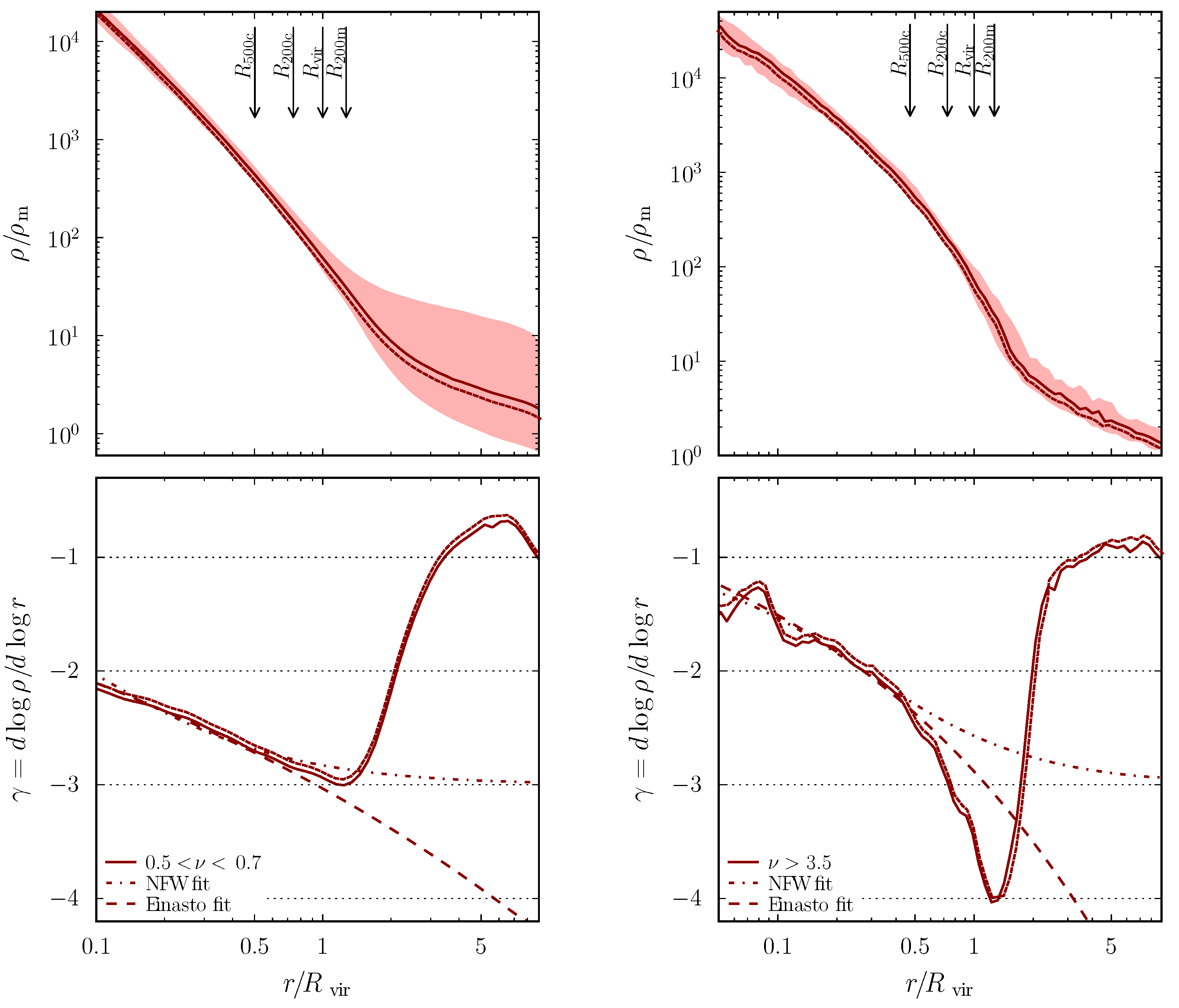
In Figure 1, we plot the median density profiles of two different halo samples, either from [19] (solid lines) or from our model (dotted lines), as well as their logarithmic slope profiles . The top panels show the median density profiles of low-mass (top left) and very massive (top right) haloes at . The shaded band represents the interval around the median containing 68% of the profiles of individual halos in the bin from [19]. The bottom panel represents the logarithmic slope profiles corresponding to the top panels. The NFW and Einasto fits of the profiles are indicated as well. The low mass sample (left panels) is characterized by , while the high mass sample contains haloes with . The solid lines represent the results from [19]. The dotted lines in the top panels represent the median density profiles while the bottom panels show the logarithmic slope profile, both obtained with our model. The plot shows a good agreement between the profiles predicted by the model and the result of the simulated model [19], only differing by a very small offset and lower numerical noise in our model’s case. The very small difference in slope cannot be perceived in the density plots. The low- sample median profile’s slope changes slowly until r ≳ Rvir. A large scatter is visible at larger radii. The high-ν sample presents a steep profile at r ≳ 0.5Rvir. The slope varies from −2 to −4 over a radius range restricted to ≈4 rescaled radius, as shown in the bottom panel representing the slope profiles. The plot shows that the NFW and Einasto profiles provide a good description of the low-ν sample out to r ≈ Rvir, while the fast steepening of the slope of the high-ν sample is poorly described. The NFW and Einasto profiles present radically different behaviors for the outer density profiles of haloes. They are able to fit the low-ν out to r ≈ Rvir for the high-ν haloes, and r ≈ 0.5Rvir in the case of the high-ν haloes. In order to fit the logarithmic slope profile, it is necessary to use a different fitting formula, such as that presented by [19] (Section 3.3 and Appendix). In the case of both the low-ν and high-ν samples, the profiles flatten to a slope of ≈−1 at r ≳ 2Rvir.
The previous plots in Figure 1 show the profiles of a bin at . In general, it could be expected that the profiles of a given when density and radii are rescaled in the correct way would be self-similar in shape. The problem is to find the radii and density to be used for rescaling.
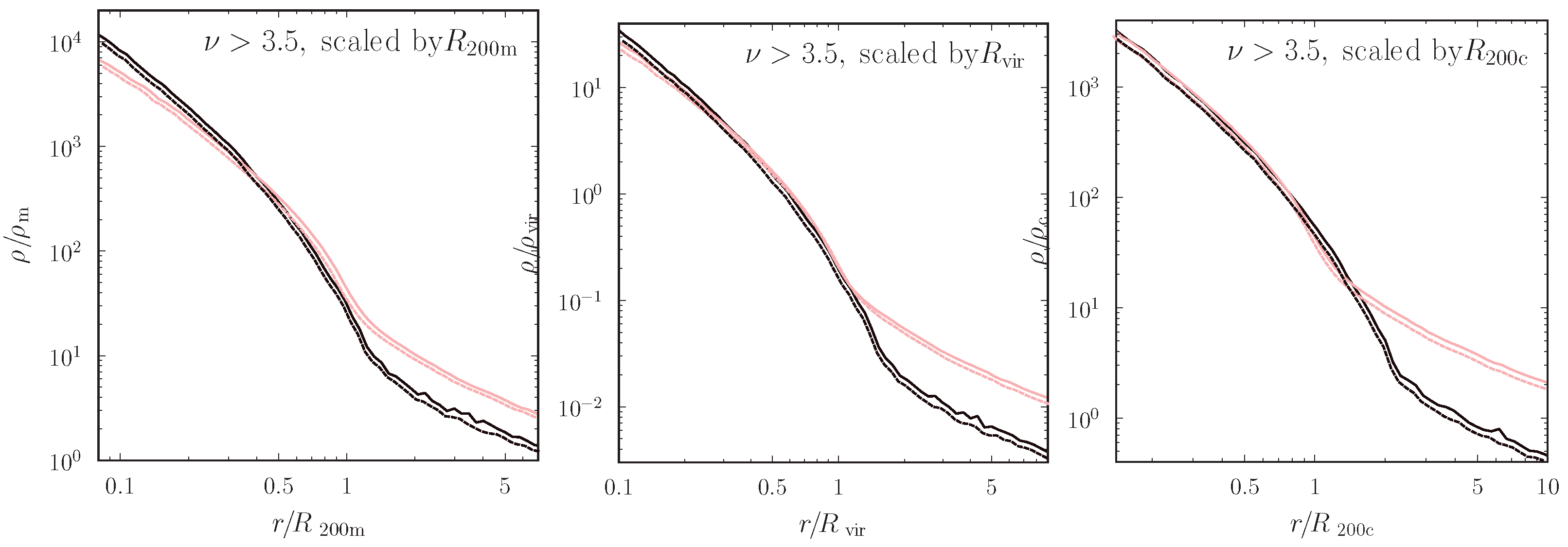
Figure 2 shows the self-similarity of the redshift evolution of the profiles for both [19] (solid lines) and for our model (dotted lines). The left panel displays the redshift evolution of the median density profiles for a peak with as a function of the radius rescaled by , with the density rescaled by . The central panel represents the same density profiles rescaled by and , respectively. The right panel represents the same density profiles rescaled by and , respectively. The black lines correspond to and the red lines to .
We emphasize that the figure plot profiles are in physical units, rescaled in the three panel from left to right by , , and , respectively, while the densities are rescaled by the corresponding quantities , , and . The plot shows clearly that the halo structure is approximately self-similar after rescaling with . It is further evident that the self-similarity depends on the kind of rescaling chosen. The most self-similar inner structures of haloes are obtained by rescaling radii and densities with and . Conversely, the most-self-similar outer profiles are obtained by rescaling with and . In order to present a more readable figure, we only plotted the haloes at two redshifts, , and . We compared the result of our model (dotted line) in Figure 3 with [19], and found again that both sets of results are in agreement, confirming the discussed self-similarity. In order to obtain a better understanding of the self-similarity, it might be possible to use logarithmic slope profiles, as they clearly reveal the radii at which rapid changes in slopes happen.
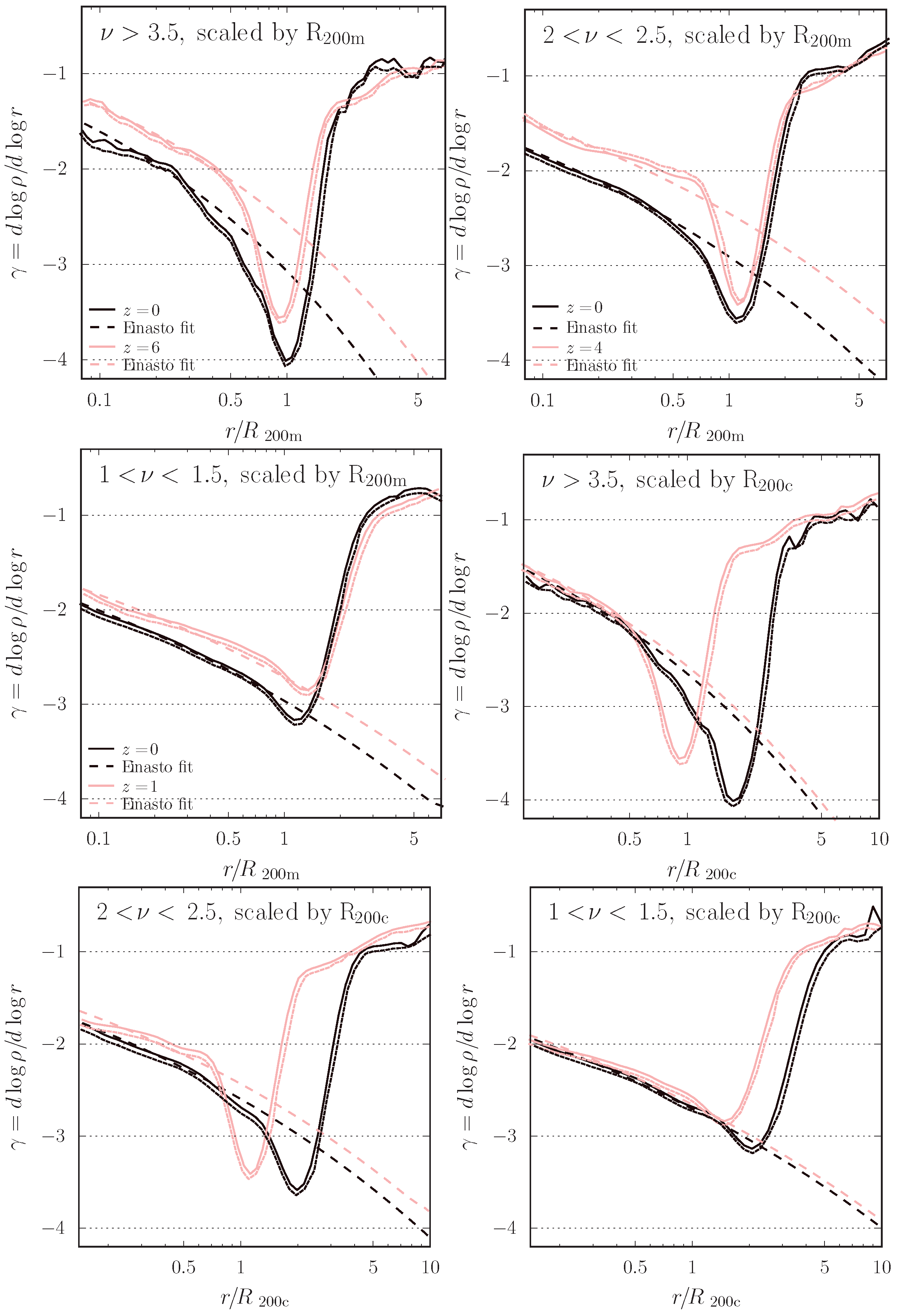
Figure 3 plots the logarithmic slope of three bins at different redshifts rescaled by (top row) and (bottom row). The left panels of Figure 3 present results for the sample of Figure 2. The central and right panels refer to the bins shown in [19], Figure 5. The radii in the top panels are rescaled in units of , while those in the bottom panel are expressed in units of . The dotted lines represent the result of our model. The solid lines stand for the [19] simulations. The dashed lines provide fits using the Einasto profile. Black and red lines correspond to different redshifts indicated in the legends of the top panels. In all cases, the slopes show a sharp steepening followed by a flattening. In units of , such sharp variations of the slope occur at the same radii with almost no sign of evolution of the transition. The radius of the steepest slope occurs around for all and redshifts. Furthermore, for haloes rescaled in units of the outer flattening displays almost no evolution or variation with . The situation is different in the case where . In this case, a variation of the slopes of the profiles at a given with and z is observed. If radii and densities are rescaled by and , the opposite is valid. While the shapes of low- and high- profiles are different, in any case they show a certain degree of uniformity at when rescaled by and at when rescaled by . The previous discussion allows us to reach the conclusion that the inner profiles are self-similar in units of while the outer profiles are self-similar in units of . It is interesting to note that one might expect a concentration of haloes to be more universal in terms of if the radius definition were related to the critical density. As in the previous figure, we only plotted two redshift dependencies in order to obtain a more readable plot. Again, the dotted lines represent the result of our model, which is in agreement with that of [19]. Another issue studied by [19] is the dependence on the mass accretion rate. As mentioned, our main goal was to show that the predictions of the simulated model [19] were in agreement with our model, that is, that our model is able to capture the main characteristics of the density profiles and their logarithmic slope to correctly describe the behavior of the outer region of the density profiles. For this reason, we do not discuss the dependence on the mass accretion rate. The comparisons shown here are sufficient to establish that our model can adequately describe the outer region of the density profile.
5. Conclusions
DM halo outskirts are characterized by very different density profiles than the inner density profile, which are usually fitted with models such as the NFW or the Einasto profile. The outer density profile is very steep over a small radial range. This kind of behavior has been interpreted as due to a pile-up of the orbits of particles and splashback of material located near half an orbit after collapse. Modeling spherical haloes, such radii provide a sharp separation of infalling matter from material just orbiting the halo, including its satellites. For exact spherical symmetry, a caustic, in this case an infinitely sharp density drop, characterises the splashback radius. In realistic halos, this caustic is smoothed out. The complexity of orbits in CDM halos along with their non-sphericity and substructures make splashback radius identification in each halo non-trivial. However, it has been observed in weak lensing as well as around stacked clusters in satellite galaxy density profiles.
Theoretically, the location of the splashback radius can be obtained through the very simple model of [20] by calculating the secondary infall of DM shell trajectories within a growing NFW-profiled DM halo. As they imposed the halo profile a priori instead of calculating it from trajectories of DM shells, they were not able to find the DM profile around the splashback radius. A more complete model was proposed by [59], who extended the self-similar collapse model of [2] to a CDM universe, allowing for simultaneous calculation of the trajectories and DM halo profile. Furthermore, [19] used simulations to study the density profiles of CDM haloes, focusing on the outer regions of the halo. They found noteworthy deviations of the outer profile from the classical distributions, such as the NFW and Einasto profiles, in the form of sharper steepening of the density profile’s logarithmic slope than had been predicted. They found that the outermost density profiles at are self-similar if the radii are rescaled by . At the same time, the inner density profiles are the most self-similar if the radii are rescaled by .
In the present paper, we have proposed an improved spherical infall model that, unlike the model of [20], takes into account shell crossing and several other effects, including ordered and random angular momentum, dynamical friction, and adiabatic contraction. Using this model, we obtained the halo density profile, and studied the behavior of the profile in its outer regions. From Gaussian initial conditions, we generated populations of haloes that can be statistically compared with other models and observations. A comparison of the profile and the logarithmic slope profile with the results of the simulations in [19] shows good agreement. We were able to reobtain the results of [19] concerning the characteristics of the density profile and its logarithmic slope.
[custom]
Author Contributions
All authors contributed equally. All authors have read and agreed to the published version of the manuscript.
Funding
MLeD acknowledges financial support by the Lanzhou University starting fund, the Fundamental Research Funds for the Central Universities (Grant No. lzujbky-2019-25), the National Science Foundation of China (grant No. 12047501), and the 111 Project under Grant No. B20063.
Institutional Review Board Statement
Not applicable.
Informed Consent Statement
Not applicable.
Data Availability Statement
Not applicable.
Conflicts of Interest
The authors declare no conflict of interest.
| 1 | RAM results from random velocities in the self-gravitating object [33]. |
| 2 | An overdense perturbation sphere within the homogeneous background Universe provides a useful non-linear model (top hat toy model). Birkhoff’s theorem is usually invoked to argue that such top hat overdensity collapses exactly as a closed sub-universe. The Newtonian approach stands on stronger justification with Gauß theorem. A more refined model divides the sphere into spherical “shells", defined as the set of particles sharing the same orbit phase at a given radius (see [39]). |
| 3 | Defined in ([8], Appendix B), with , and , the mass variance averaged on a scale . |
| 4 | For precision’s sake, the mass scale M is connected to the smoothing scale by for Gaussian smoothing () and by for top hat smoothing. The mass enclosed by the smoothing function applied to the uniform background is the same for (see BBKS). |
References
- Gunn, J.E.; Gott, J.R., III. On the Infall of Matter Into Clusters of Galaxies and Some Effects on Their Evolution. Astrophys. J. 1972, 176, 1. [Google Scholar] [CrossRef]
- Fillmore, J.A.; Goldreich, P. Self-similar gravitational collapse in an expanding universe. Astrophys. J. 1984, 281, 1. [Google Scholar] [CrossRef]
- Hoffman, Y.; Shaham, J. Local density maxima: Progenitors of structure. Astrophys. J. 1985, 297, 16. [Google Scholar] [CrossRef]
- Popolo, A.D.; Gambera, M. Substructure effects on the collapse of density perturbations. Astrophysics 1997, 321, 691. [Google Scholar]
- Ascasibar, Y.; Yepes, G.; Gottlober, S.; Muller, V. On the physical origin of dark matter density profiles. Mon. Not. R. Astron. Soc. 2004, 352, 1109. [Google Scholar] [CrossRef]
- Williams, L.L.R.; Babul, A.; Dalcanton, J.J. Investigating the Origins of Dark Matter Halo Density Profiles. Astrophys. J. 2004, 604, 18. [Google Scholar] [CrossRef]
- Hiotelis, N.; Popolo, A.D. On the Reliability of Merger-Trees and the Mass-Growth Histories of Dark Matter Haloes. Astrophys. Space Sci. 2006, 301, 167. [Google Scholar] [CrossRef]
- Del Popolo, A. The cusp/core problem and the secondary infall model. Astrophys. J. 2009, 698, 2093. [Google Scholar] [CrossRef]
- Cardone, V.F.; Leubner, M.P.; Popolo, A.D. Spherical galaxy models as equilibrium configurations in non-extensive statistics. Mon. Not. R. Astron. Soc. 2011, 414, 2265. [Google Scholar] [CrossRef]
- Blumenthal, G.R.; Faber, S.M.; Flores, R.; Primack, J.R. Contraction of Dark Matter Galactic Halos Due to Baryonic Infall. Astrophys. J. 1986, 301, 27. [Google Scholar] [CrossRef]
- Gnedin, O.Y.; Kravtsov, A.V.; Klypin, A.A.; Nagai, D. Response of dark matter halos to condensation of baryons: Cosmological simulations and improved adiabatic contraction model. Astrophysics 2004, 616, 16. [Google Scholar] [CrossRef]
- Gustafsson, M.; Fairbairn, M.; Sommer-Larsen, J. Baryonic pinching of galactic dark matter halos. Phys. Rev. D 2006, 74, 123522. [Google Scholar] [CrossRef]
- Navarro, J.F.; Frenk, C.S.; White, S.D.M. The Structure of Cold Dark Matter Halos. Astrophys. J. 1996, 462, 563. [Google Scholar] [CrossRef]
- Navarro, J.F.; Frenk, C.S.; White, S.D.M. A Universal Density Profile from Hierarchical Clustering. Astrophys. J. 1997, 490, 493. [Google Scholar] [CrossRef]
- Merritt, D.; Navarro, J.F.; Ludlow, A.; Jenkins, A. A Universal Density Profile for Dark and Luminous Matter? Astrophys. J. 2005, 624, L85. [Google Scholar] [CrossRef]
- Navarro, J.F.; Ludlow, A.; Springel, V.; Wang, J.; Vogelsberger, M.; White, S.D.M.; Jenkins, A.; Frenk, C.S.; Helmi, A. The diversity and similarity of simulated cold dark matter haloes. Mon. Not. R. Astron. Soc. 2010, 402, 21. [Google Scholar] [CrossRef]
- Cintio, A.D.; Brook, C.B.; Dutton, A.A.; Macci‘o, A.V.; Stinson, G.S.; Knebe, A. A mass-dependent density profile for dark matter haloes including the influence of galaxy formation. Mon. Not. R. Astron. Soc. 2014, 441, 2986. [Google Scholar] [CrossRef]
- Freundlich, J.; Jiang, F.; Dekel, A.; Cornuault, N.; Ginzburg, O.; Koskas, R.; Lapiner, S.; Dutton, A.; Macci‘o, A.V. The Dekel-Zhao profile: A mass-dependent dark-matter density profile with flexible inner slope and analytic potential, velocity dispersion, and lensing properties. Mon. Not. R. Astron. Soc. 2020, 499, 2912. [Google Scholar] [CrossRef]
- Diemer, B.; Kravtsov, A.V. Dependence of the outer density profiles of halos on their mass accretion rate. Astrophys. J. 2014, 789, 1. [Google Scholar] [CrossRef]
- Adhikari, S.; Dalal, N.; Chamberlain, R.T. Splashback in accreting dark matter halos. J. Cosmol. Astropart. Physics 2014, 2014, 19. [Google Scholar] [CrossRef]
- Lithwick, Y.; Dalal, N. Self-similar solutions of triaxial dark matter halos. Astrophys. J. 2011, 734, 100. [Google Scholar] [CrossRef]
- Cooper, A.P.; Mart´ınez-Delgado, D.; Helly, J.; Frenk, C.; Cole, S.; Crawford, K.; Zibetti, S.; Carballo-Bello, J.A.; GaBany, R.J. The formation of shell galaxies similar to ngc 7600 in the cold dark matter cosmogony. Astrophys. J. Lett. 2011, 743, L21. [Google Scholar] [CrossRef]
- Diemand, J.; Kuhlen, M. Infall Caustics in Dark Matter Halos? Astrophys. J. 2008, ApJL 680, L25. [Google Scholar] [CrossRef]
- Vogelsberger, M.; Mohayaee, R.; White, S.D.M. Non-spherical similarity solutions for dark halo formation. Mon. Not. R. Astron. Soc. 2011, 414, 3044. [Google Scholar] [CrossRef]
- Del Popolo, A. On the universality of density profiles. Mon. Not. R. Astron. Soc. 2010, 408, 1808. [Google Scholar] [CrossRef]
- Del Popolo, A. Non-power law behavior of the radial profile of phase-space density of halos. J. Cosmol. Astropart. Phys. 2011, 2011, 14. [Google Scholar] [CrossRef]
- Del Popolo, A. Density profile slopes of dwarf galaxies and their environment. Mon. Not. R. Astron. Soc. 2012, 419, 971–984. [Google Scholar] [CrossRef]
- Del Popolo, A. Nonbaryonic dark matter in cosmology. Int. J. Mod. Phys. 2014, 23, 1430005. [Google Scholar] [CrossRef]
- Del Popolo, A. On the density-profile slope of clusters of galaxies. Mon. Not. R. Astron. Soc. 2012, 424, 38. [Google Scholar] [CrossRef]
- Popolo, A.D.; Cardone, V.F.; Belvedere, G. Surface density of dark matter haloes on galactic and cluster scales. Mon. Not. R. Astron. Soc. 2013, 429, 1080. [Google Scholar] [CrossRef]
- Popolo, A.D.; Pace, F.; Lima, J.A.S. Extended spherical collapse and the accelerating universe. Int. J. Mod. Phys. 2013, 22, 1350038. [Google Scholar] [CrossRef] [Green Version]
- Popolo, A.D.; Pace, F.; Lima, J.A.S. Spherical collapse model with shear and angular momentum in dark energy cosmologies. Mon. Not. R. Astron. Soc. 2013, 430, 628. [Google Scholar] [CrossRef]
- Ryden, B.S.; Gunn, J.E. Galaxy Formation by Gravitational Collapse. Astrophys. J. 1987, 318, 15. [Google Scholar] [CrossRef]
- Gurevich, A.V.; Zybin, K.P. Syunyaev. Zhurnal Eksperimental noi i Teoreticheskoi Fiziki 1988, 94, 3, 5. [Google Scholar]
- White, S.D.M.; Zaritsky, D. Models for Galaxy Halos in an Open Universe. Astrophys. J. 1992, 394, 1. [Google Scholar] [CrossRef]
- Sikivie, P.; Tkachev, I.I.; Wang, Y. Secondary infall model of galactic halo formation and the spectrum of cold dark matter particles on Earth. Phys. Rev. D 1997, 56, 1863. [Google Scholar] [CrossRef]
- Nusser, A. Self-similar spherical collapse with non-radial motions. Mon. Not. R. Astron. Soc. 2001, 325, 1397. [Google Scholar] [CrossRef]
- Hiotelis, N. Density profiles in a spherical infall model with non–radial motions. A&A 2002, 382, 84. [Google Scholar]
- Delliou, M.L.; Henriksen, R.N. Non-radial motion and the NFW profile. A&A 2003, 408, 27. [Google Scholar]
- Zukin, P.; Bertschinger, E. A Generalized Secondary Infall Model. American Physical Society, APS Meeting Abstracts. 2010, p. 13003. Available online: https://hal.archives-ouvertes.fr/hal-00000474/document (accessed on 4 August 2022).
- Peebles, P.J.E. Origin of the Angular Momentum of Galaxies. Astrophys. J. 1969, 155, 393. [Google Scholar] [CrossRef]
- White, S.D.M. Angular momentum growth in protogalaxies. Astrophys. J. 1984, 286, 38. [Google Scholar] [CrossRef]
- Antonuccio-Delogu, V.; Colafrancesco, S. Dynamical Friction, Secondary Infall, and the Evolution of Clusters of Galaxies. Astrophys. J. 1994, 427, 72. [Google Scholar] [CrossRef]
- El-Zant, A.; Shlosman, I.; Hoffman, Y. Dark Halos: The Flattening of the Density Cusp by Dynamical Friction. Astrophys. J. 2001, 560, 636. [Google Scholar] [CrossRef]
- El-Zant, A.A.; Hoffman, Y.; Primack, J.; Combes, F.; Shlosman, I. Flat-cored Dark Matter in Cuspy Clusters of Galaxies. Astrophys. J. 2004, 607, L75. [Google Scholar] [CrossRef]
- Gunn, J.E. Massive galactic halos. I. Formation and evolution. Astrophys. J. 1977, 218, 592. [Google Scholar] [CrossRef]
- Peebles, P.J.E. The Large-Scale Structure of the Universe; Princeton University Press: Princeton, NJ, USA, 1980. [Google Scholar]
- Zaroubi, S.; Naim, A.; Hoffman, Y. Secondary Infall: Theory versus Simulations. Astrophys. J. 1996, 457, 50. [Google Scholar] [CrossRef]
- Zaroubi, S.; Hoffman, Y. Gravitational Collapse in an Expanding Universe: Asymptotic Self-similar Solutions. Astrophys. J. 1993, 416, 410. [Google Scholar] [CrossRef]
- Łokas, E.L. Universal profile of dark matter haloes and the spherical infall model. Mon. Not. R. Astron. Soc. 2000, 311, 423. [Google Scholar] [CrossRef]
- Hoyle, F. On the Fragmentation of Gas Clouds Into Galaxies and Stars. Astrophys. J. 1953, 118, 513. [Google Scholar] [CrossRef]
- Ryden, B.S. Galaxy Formation: The Role of Tidal Torques and Dissipational Infall. Astrophys. J. 1988, 329, 589. [Google Scholar] [CrossRef]
- Eisenstein, D.J.; Loeb, A. An Analytical Model for the Triaxial Collapse of Cosmological Perturbations. Astrophys. J. 1995, 439, 520. [Google Scholar] [CrossRef]
- Avila-Reese, V.; Firmani, C.; Hern´andez, X. On the Formation and Evolution of Disk Galaxies: Cosmological Initial Conditions and the Gravitational Collapse. Astrophys. J. 1998, 505, 37. [Google Scholar] [CrossRef]
- Bardeen, J.M.; Bond, J.R.; Kaiser, N.; Szalay, A.S. The Statistics of Peaks of Gaussian Random Fields. Astrophys. J. 1986, 304, 15. [Google Scholar] [CrossRef]
- Spergel, D.N.; Bean, R.; Dor´e, O.; Nolta, M.R.; Bennett, C.L.; Dunkley, J.; Hinshaw, G.; Jarosik, N.; Komatsu, E.; Page, L.; et al. Three-Year Wilkinson Microwave Anisotropy Probe (WMAP) Observations: Implications for Cosmology. Astrophys. J. Suppl. Ser. 2007, 170, 377. [Google Scholar] [CrossRef] [Green Version]
- Eisenstein, D.J.; Hu, W. Baryonic Features in the Matter Transfer Function. Astrophys. J. 1998, 496, 605. [Google Scholar] [CrossRef]
- Savitzky, A.; Golay, M.J.E. Smoothing and differentiation of data by simplified least squares procedures. Anal. Chem. 1964, 36, 1627. [Google Scholar] [CrossRef]
- Shi, X. The outer profile of dark matter haloes: An analytical approach. Mon. Not. R. Astron. Soc. 2016, 459, 3711. [Google Scholar] [CrossRef] [Green Version]
Figure 1.
Median density profiles of low-mass (top left) and very massive haloes (top right) at . The shaded band represents the interval around the median containing 68% of the profiles of individual halos in the bin. The bottom panel shows the logarithmic slope profiles from the top panel profiles. The NFW and Einasto fits of the profiles are indicated as well. The solid lines represent the results from [19]. The dotted lines in the top panels represent the median density profiles, while the bottom panels show the logarithmic slope profile, both obtained with our model.

Figure 2.
Self-similarity of the redshift evolution of the profiles. In all panels, solid lines represent the results from [19] while dotted lines show results obtained with our model. Left panel: redshift evolution of the median density profiles for a peak with as a function of the radius rescaled by and with density rescaled by . Central panel: the same density profiles rescaled by and , respectively. Right panel: the same density profiles rescaled by , and , respectively. The black lines correspond to and the red lines to .

Figure 3.
Logarithmic slope of three bins at different redshifts. The left panels are related to the sample of Figure 2. The central, and right panels refer to the bins shown in [19], Figure 5. The radii in the top panels are rescaled in units of , while those in the bottom panel are expressed in units of . Again, the solid lines stand for the simulations in [19], the dashed lines provide fits using the Einasto profile, and the dotted lines represents the result of our model. The black and red lines correspond to different redshifts indicated in the legends of the top panels.

Publisher’s Note: MDPI stays neutral with regard to jurisdictional claims in published maps and institutional affiliations. |
© 2022 by the authors. Licensee MDPI, Basel, Switzerland. This article is an open access article distributed under the terms and conditions of the Creative Commons Attribution (CC BY) license (https://creativecommons.org/licenses/by/4.0/).
Share and Cite
MDPI and ACS Style
Del Popolo, A.; Le Delliou, M. Splashback Radius in a Spherical Collapse Model. Universe 2022, 8, 462. https://doi.org/10.3390/universe8090462
AMA Style
Del Popolo A, Le Delliou M. Splashback Radius in a Spherical Collapse Model. Universe. 2022; 8(9):462. https://doi.org/10.3390/universe8090462
Chicago/Turabian StyleDel Popolo, Antonino, and Morgan Le Delliou. 2022. "Splashback Radius in a Spherical Collapse Model" Universe 8, no. 9: 462. https://doi.org/10.3390/universe8090462
Note that from the first issue of 2016, this journal uses article numbers instead of page numbers. See further details here.