the Creative Commons Attribution 4.0 License.
the Creative Commons Attribution 4.0 License.
 | 06 Sep 2022
A 500-year annual runoff reconstruction for 14 selected European catchments
Sadaf Nasreen
Markéta Součková
Mijael Rodrigo Vargas Godoy
Ujjwal Singh
Yannis Markonis
Rohini Kumar
Oldrich Rakovec
Since the beginning of this century, Europe has been experiencing severe drought events (2003, 2007, 2010, 2018 and 2019) which have had adverse impacts on various sectors, such as agriculture, forestry, water management, health and ecosystems. During the last few decades, projections of the impact of climate change on hydroclimatic extremes have often been used for quantification of changes in the characteristics of these extremes. Recently, the research interest has been extended to include reconstructions of hydroclimatic conditions to provide historical context for present and future extremes. While there are available reconstructions of temperature, precipitation, drought indicators, or the 20th century runoff for Europe, multi-century annual runoff reconstructions are still lacking. In this study, we have used reconstructed precipitation and temperature data, Palmer Drought Severity Index and available observed runoff across 14 European catchments in order to develop annual runoff reconstructions for the period 1500–2000 using two data-driven and one conceptual lumped hydrological model. The comparison to observed runoff data has shown a good match between the reconstructed and observed runoff and their characteristics, particularly deficit volumes. On the other hand, the validation of input precipitation fields revealed an underestimation of the variance across most of Europe, which is propagated into the reconstructed runoff series. The reconstructed runoff is available via Figshare, an open-source scientific data repository, under the DOI https://doi.org/10.6084/m9.figshare.15178107, (Sadaf et al., 2021).
- Article
(11106 KB) - Full-text XML
-
Supplement
(664 KB) - BibTeX
- EndNote


Global warming has impacted numerous land surface processes (Reinecke et al., 2021) over the last few decades, resulting in more severe droughts, heatwaves, floods and other extreme events. Droughts, in particular, pose a serious threat to Europe's water resources. The flow of many rivers is greatly hampered by prolonged droughts, which restrain the availability of fresh water for agriculture and domestic use. For example, the 2003 drought significantly reduced European river flows by approximately 60 % to 80 % relative to the average (Zappa and Kan, 2007). Likewise, the annual flow levels at several river gauges have decreased by 9 % to 22 % over the last decade (Middelkoop et al., 2001; Krysanova et al., 2008; Uehlinger et al., 2009; Su et al., 2020) due to a lack of rainfall and a warmer climate.
While runoff is a key element related to water security, it is challenging to interpret recent hydroclimate fluctuations (multi-year droughts in particular) considering observed runoff records (Markonis and Koutsoyiannis, 2016; Hanel et al., 2018), which are in general seldom available for years prior to 1900. In this way, the community does not have runoff information on various severe multi-year droughts and pluvial periods, which can be assessed only indirectly using (typically seasonal or annual) reconstructions based on various proxy data, such as past tree rings (Nicault et al., 2008; Kress et al., 2010; Cook et al., 2015; Tejedor et al., 2016; Casas-Gómez et al., 2020), speleothem (Vansteenberge et al., 2016), ice cores, sediments (Luoto and Nevalainen, 2017), and documentary and instrumental evidence (Pfister et al., 1999; Brázdil and Dobrovolný, 2009; Dobrovolný et al., 2010; Wetter et al., 2011).
The majority of existing reconstructions focus on temperature (Luterbacher et al., 2004; Xoplaki et al., 2005; Casty et al., 2005; Büntgen et al., 2006; Moberg et al., 2008; Dobrovolný et al., 2010; Trouet et al., 2013; Emile-Geay et al., 2017), precipitation (Wilson et al., 2005; Boch and Spötl, 2011; Wilhelm et al., 2012; Murphy et al., 2018) or droughts (Büntgen et al., 2010; Kress et al., 2014; Cook et al., 2015; Tejedor et al., 2016; Ionita et al., 2017; Brázdil et al., 2018; Hanel et al., 2018) and floods (Wetter et al., 2011; Swierczynski et al., 2012). A few studies have been conducted for the reconstruction of runoff–drought deficit series (Hansson et al., 2011; Kress et al., 2014; Hanel et al., 2018; Moravec et al., 2019; Martínez-Sifuentes et al., 2020). However, these studies are either local or regional or cover a relatively short period. As an example, Hansson et al. (2011) introduced a runoff series for the Baltic Sea from the years 1550 to 1995 using temperature and atmospheric circulation indices. Similarly, Sun et al. (2013) used tree-ring proxies to reconstruct runoff in the Fenhe River basin in China's Shanxi region over the last 211 years. As another example, Caillouet et al. (2017) provide a 140-year dataset of reconstructed streamflow over 662 natural catchments in France since 1871 using the GR6J hydrological model, highlighting several well-known extreme low-flow events. A multi-ensemble modelling approach using GR4J has been applied by Smith et al. (2019) to develop UK-based historical river flows and examine the potential of reconstruction for capturing peak- and low-flow events from 1891 to 2015.
The available reconstructed precipitation and temperature series (or fields) can be used to reconstruct runoff with hydrological (process-based) models (Tshimanga et al., 2011; Armstrong et al., 2020) respecting general physical laws, such as preserving mass balance (e.g. MIKE SHE; Im et al., 2009 or VELMA; Laaha et al., 2017) or data-driven methods which are able to capture complex non-linear relationships (for instance support vector machines, Zuo et al., 2020; Ji et al., 2021; artificial neural networks (ANNs), Senthil Kumar et al., 2005; Hu et al., 2018; Kwak et al., 2020; random forests, Ghiggi et al., 2019; Li et al., 2021; Contreras et al., 2021). While the lack of physical constraints in the data-driven models limits their application under changing boundary conditions (in comparison with those of the model training period), their advantage is that they can often directly use biased reconstructed data as an input series.
The objective of the present study is to provide a multi-century annual runoff reconstruction for 14 European catchments, utilizing the available precipitation (P; Pauling et al., 2006) and temperature (T; Luterbacher et al., 2004) reconstructions and the Old World Drought Atlas self-calibrated Palmer Drought Severity Index (scPDSI) reconstruction (Cook et al., 2015). Specifically, we assessed a conceptual lumped hydrological model (GR1A; Mouelhi et al., 2006) and two data-driven models, long short-term memory neural network (LSTM; Chen et al., 2020) and Bayesian regularized neural network (BRNN; Okut, 2016), for annual runoff simulation over the period 1500–2000.
Section 2 introduces P and T hydroclimatic reconstructions and the scPDSI drought indicator as well as precipitation, temperature and runoff observations. In Sect. 3, we describe the data preprocessing, models, the drought identification methodology and goodness-of-fit assessment. The accuracy of the employed P and T reconstructions, as well as the derived runoff simulations, is evaluated in Sect. 4. Finally, we summarize the advantages and limitations of reconstructed datasets in the Conclusions in Sect. 6.
Pauling et al. (2006)Luterbacher et al. (2004)Menne et al. (2018)Menne et al. (2018)Cook et al. (2015)
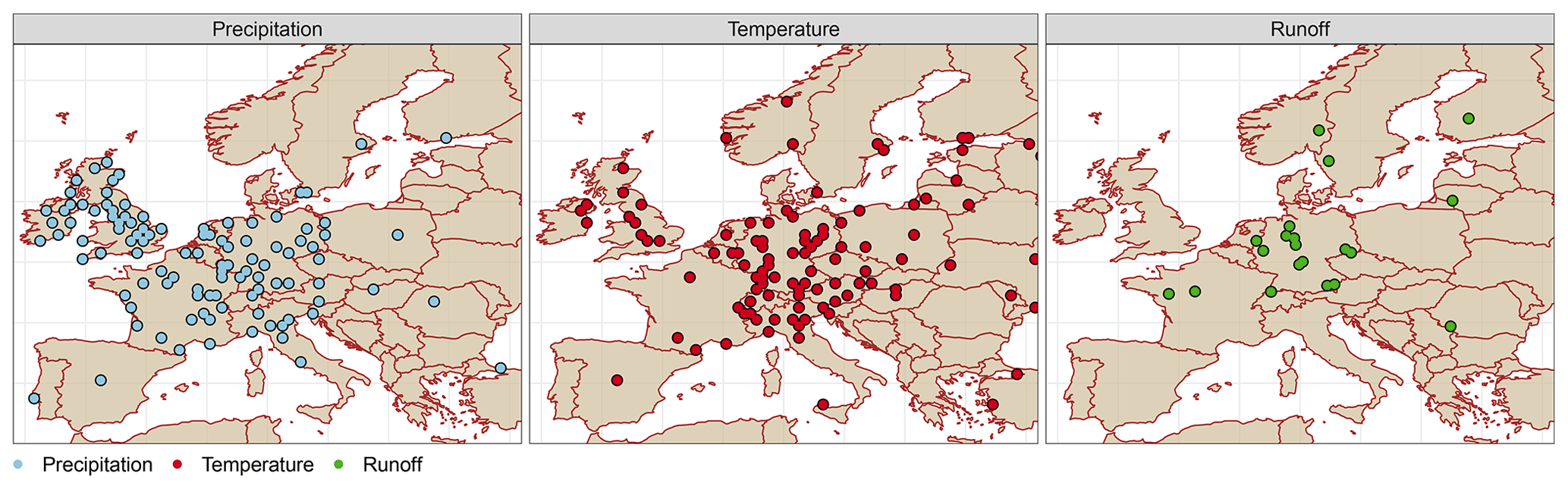
Figure 1Spatial distribution of the observed GHCN precipitation and temperature stations and GRDC runoff gauges.
This section presents the data used in this study. To force the models, we investigated the use of precipitation (Pauling et al., 2006) and temperature (Luterbacher et al., 2004) reconstructions for the past half-millennium and scPDSI drought indicator data from the Old World Drought Atlas (Cook et al., 2015). For validating the runoff reconstructions, we used runoff from the Global Runoff Data Center (GRDC; Fekete et al., 1999). The accuracy of atmospheric forcing reconstruction used as model input was assessed using the observational data records of P and T from the Global Historical Climatology Network (GHCN; Menne et al., 2018). The datasets are summarized in Table 1 and are described in more detail below.
2.1 Precipitation
We used reconstructed seasonal precipitation (0.5∘ × 0.5∘) over Europe (30.25–70.75∘ N, 29.75∘ W–39.75∘ E) from 1500 to 2000. Reconstructed precipitation (P) was derived by Pauling et al. (2006) through principal component regression based on documented evidence (i.e. memoirs, annals and newspapers), speleothem proxy records (Proctor et al., 2000) and tree-ring chronologies from the International Tree-Ring Data Bank (ITRDB; Jeong et al., 2021) .
2.2 Temperature
Reconstructed temperature (T) was obtained from Luterbacher et al. (2004), which relies on historical records and seasonal natural proxies (i.e. ice cores from Greenland and tree rings from Scandinavia and Siberia). Reconstructed temperature data are available at the same spatial and temporal resolution as precipitation (see Table 1). We refer to both of these datasets as reconstructed forcings or reconstructed precipitation/temperature fields.
2.3 Self-calibrating Palmer Drought Severity Index (scPDSI)
In addition, we used data from the Old World Drought Atlas (OWDA; Cook et al., 2015) which contains information regarding moisture conditions across Europe, specifically the self-calibrated Palmer Drought Severity Index (scPDSI) using summer-related tree-ring proxies over the period 0 to 2012 CE.
2.4 The Global Historical Climatology Network (GHCN)
The GHCN dataset (GHCN; Peterson and Vose, 1997) is one of the largest observational databases, collated by the National Oceanic and Atmospheric Administration (NOAA; Quayle et al., 1999). The GHCN-m dataset contains observed temperature, rainfall and pressure data from 1701 to 2010. Data for the majority of stations are, however, available after 1900. GHCN-m precipitation and temperature from GHCN V2, as well as from the GHCN V4 version (Menne et al., 2012), were used to assess the reconstruction accuracy of the P and T fields as an input into the considered models. We selected 113 precipitation and 144 temperature stations within the European domain (see Fig. 1) with records dating back earlier than 1875. Most stations are geographically concentrated in central Europe, and few stations are located in the eastern and northern areas of Europe (see Table 2). These data, hereafter, are referred to as the GHCN data.
2.5 Observed runoff
The Global Runoff Data Center (GRDC; http://www.bafg.de/GRDC/EN/Home/homepage_node.html, last access: 24 November 2016) provides data for more than 2780 gauging stations in Europe, with the oldest records starting from 1806. Only the GRDC runoff time series with at least 25 years of data prior to 1900 were selected. In total, there were 21 such stations predominantly available in central Europe: 11 in Germany, 2 in France, 2 in Switzerland, 1 in the Czech Republic, 1 in Sweden, 1 in Finland, 1 in Lithuania and 1 in Romania (see Fig. 1). These stations cover 12 European river basins (Rhine, Loire, Elbe, Danube, Wesser, Main, Glama, Slazach, Nemunas, Gota Alv, Inn and Kokemaenjoke), with areas ranging from nearly 6100 km2 (Kokemaenjoki, Muroleenkoski, Finland) to 576 000 km2 (Danube, Orsova, Romania). The mean annual discharge (Qmean) varies from 50 to 5 600 m3 s−1 and spans different time periods for each catchment.
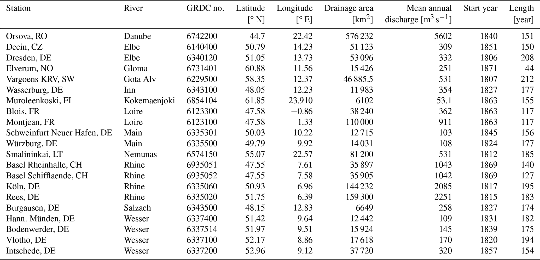
The most extensive records were available in Sweden (Vargoens KRV) and Germany (Dresden), containing the longest discharge series of 212 and 208 years, respectively. The gauging station in Köln also provided 195 years of data for the Rhine River. Note that some of the gauging stations are located nearby and therefore have a greater degree of similarity in their runoff time series (e.g. two stations in Basel, Rhine). Detailed information relating to all selected stations is provided in Table 2.
2.6 Study area
In the first part of the study, the grid-based reconstruction of precipitation and temperature was verified against the available GHCN data across the European region bounded by (30.25–70.75∘ N, 29.75∘ W–39.75∘ E). The second part focused on 21 specific central European catchments, corresponding to the available long-term GRDC discharge records. The study area and the observational data of the hydroclimatic variables are shown in Fig. 2.
This section is divided into three parts. The first part describes the preprocessing of the reconstructed forcings (i.e. precipitation and temperature) for validation across Europe and the preparation of data for runoff simulation in 21 catchments (Sect. 3.1). The hydrologic and data-driven models used to generate the runoff reconstructions are presented in Sect. 3.2 and 3.3, respectively. Finally, Sect. 3.4 describes the methods for the evaluation of simulated runoff and reconstructed forcings, and Sect. 3.5 presents the methods to identify annual runoff droughts.
3.1 Data preprocessing
Two databases were considered for the analysis and development of the annual runoff reconstruction. The first one was used for evaluating the accuracy of meteorological forcing reconstructions used for hydrological simulations and consists of observed GHCN data for all available European stations with long records (see Sect. 2.4) and values of corresponding grid cells from the reconstructed forcings dataset.
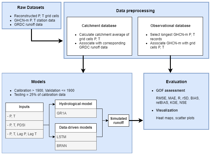
The second database was created as the basis for runoff reconstruction containing the observed runoff data for 21 selected catchments (Table 2) and the corresponding input variables of the models used to generate the multi-century runoff reconstructions. Several input variables were considered for inclusion in models such as reconstructed precipitation and temperature and Old World Drought Atlas scPDSI. The catchment average precipitation, temperature and scPDSI were estimated from the corresponding (gridded) datasets by averaging the relevant grid cells over the catchments. This database was further divided into two parts, calibration (1900–2000) and validation (before 1900), to assess the model's accuracy and to select an appropriate model. The data preprocessing, model selection, and evaluation of the models are depicted in Fig. 2.
3.2 Hydrologic model (GR1A)
We applied the annual timescale hydrologic model, GR1A (Mouelhi et al., 2006), to simulate annual runoff in each catchment. GR1A is a conceptual lumped hydrologic model (Manabe, 1969), considering dynamic storage and antecedent precipitation conditions. The model consists of a simple mathematical equation with a single (optimized) parameter:
where Q, E and P represent annual runoff, basin average potential evapotranspiration and basin average precipitation, respectively, and i denotes the year. The parameter X is optimized individually for each catchment by maximizing the Nash–Sutcliffe efficiency (NSE) between observed and simulated runoff. Default gradient-based optimization from the R package airGR (Coron et al., 2017) was used. The potential evapotranspiration was calculated using the temperature-based formula (Oudin et al., 2005). Compared to other conceptual models from the GR family (GR4J, GR5J), GR1A is simple to use, and it allows for analysing many variants, particularly defining the best antecedent rainfall, and is potentially useful to predict wet and dry hydrologic conditions (Mouelhi et al., 2006).
3.3 Data-driven models
Artificial neural networks (ANNs; Senthil Kumar et al., 2005; Kwak et al., 2020) can describe non-linear relationships and are widely used for rainfall–runoff prediction. The ANNs consist of artificial neurons organized in layers and connections that route the signal through the network. Each connection has an associated weight that is optimized within the calibration (in the context of ANNs, known as training). There are many types of ANNs which differ in terms of structure and type of connections, as well as direction and functional forms used for neuron activation or training. In the present study, we considered two approaches: long short-term memory (LSTM) neural networks and Bayesian regularized neural networks (BRNNs). These approaches have been commonly used in past rainfall–runoff modelling studies (Hu et al., 2018; Kratzert et al., 2018; Xiang et al., 2020; Ye et al., 2021). We considered combinations of reconstructed forcing, OWDA-based scPDSI and lagged forcing as an input into the network for both model types. Specifically, the network using only reconstructed precipitation and temperature fields is referred to as [P,T], the network with reconstructed forcing and OWDA scPDSI is termed as ; and finally the network which includes 1-year lagged P and T forcing in addition to actual P and T is referred to as . We also considered and explored lag times longer than 1 year. However the correlation between precipitation and runoff drops significantly at lag times longer than 1 year and therefore was not included in presented analysis.
Figure A1 shows the architecture of LSTM, which is a modified version of the recurrent neural network (Hochreiter and Schmidhuber, 1997), using backpropagation in time (Werbos, 1990). LSTM is known for efficient simulation of time series with long-term memory (Van Houdt et al., 2020). It generally consists of two unit states (hidden and cell states) and three distinct gates (hidden, input and output). In this process, the cell state saves the long-term memory at the previous unit, while hidden states act as a working memory to process information inside the gates. These gates can determine which information needs to be processed, remembered and transferred in the next state. With LSTM, different activation functions, such as hyperbolic tangent and sigmoid, can be used to update unit states. The implementation of the LSTM is carried out by applying the R packages “keras” (Arnold, 2017) and “tensorflow” (Abadi et al., 2016).
The training process of the LSTM is time-consuming due to its inherent complexity. Therefore we also considered the BRNN models that provide fast learning and convergence and were already used to tackle the complex relationship between rainfall and runoff (Ye et al., 2021). BRNNs are based on recurrent neural networks, which are often used to model time-series data (Wang et al., 2007), and the methods are extended with Bayesian regularization (Okut, 2016) to account for uncertainty related to network parameters and input data (Zhang et al., 2011). We trained this model in R using the “brnn” function of the “caret” package (Kuhn, 2015). More details are available in Appendix A3.
To set the optimal hyperparameters of the models (such as the number of neurons and activation functions) and to reduce the likelihood of overfitting during the calibration/training, the model performance was cross-checked considering an independent (or so-called “testing”) set. The testing set was for each learning exercise extracted from the calibration data (1900–2000) as a random fraction (25 %). This process of the model development was repeated several times, minimizing the root mean square error (for BRNN) and mean square error (for LSTM) for each catchment individually. The model with the best performance was then chosen for further evaluation.
3.4 Goodness-of-fit assessment
We used a set of seven statistical metrics to assess the performance of simulated runoff, namely Nash–Sutcliffe efficiency (NSE), Pearson correlation (R), standard deviation ratio (rSD), Kling–Gupta efficiency (KGE), root mean square error (RMSE), mean absolute error (MAE), bias (BIAS) and relative bias (relBIAS). The mathematical formulations of these metrics are provided in Appendix A1.
3.5 Runoff drought identification
To check the utility of our reconstruction, we finally explore how well the annual runoff droughts are represented in the simulations. Our study considers annual hydrological droughts, defined as the streamflow/runoff deficit, following the threshold level approach (Yevjevich, 1967; Sung and Chung, 2014; Rivera et al., 2017). This approach is typically used for daily or monthly timescales, considering 0.1 or 0.2 quantile threshold levels. To accommodate the annual scale used here, we defined the start of the drought, when the annual runoff anomaly falls below the 0.33 quantile (regular drought) and the 0.05 quantile (extreme drought). The drought persists until the runoff rises above the threshold again. After that, the difference between runoff and the threshold was determined for each identified drought year, called the runoff deficit. Hydrological drought series can be further assessed to understand the critical aspects of runoff (temporal) dynamics and to classify past droughts in Europe (Wetter and Pfister, 2013; Cook et al., 2015).
In this section, we analyse the 500-year annual reconstruction over space and time across Europe. Firstly, we provide a comparison between the GHCN-observed precipitation and temperature and the corresponding grid cells from Pauling et al. (2006) and Luterbacher et al. (2004) reconstructions. Next, the reconstructed annual runoff series for the selected catchments are evaluated against the corresponding observed GRDC runoff data.
Two distinct model types were investigated, i.e. a process-based conceptual lumped hydrological model (GR1A) and two data-driven models (BRNN and LSTM). While the former takes reconstructed forcing of precipitation and temperature as an input, in the case of the latter, we also considered PDSI and lagged reconstructed precipitation and temperature fields, as shown in Table 3. Statistical metrics, such as NSE, KGE, RMSE, MAE, R, BIAS and relBIAS (Appendix A1), are used to quantify the predictive skills of the models examined.

Figure 3Validation of reconstructed precipitation (Pauling et al., 2006) against GHCN observations.
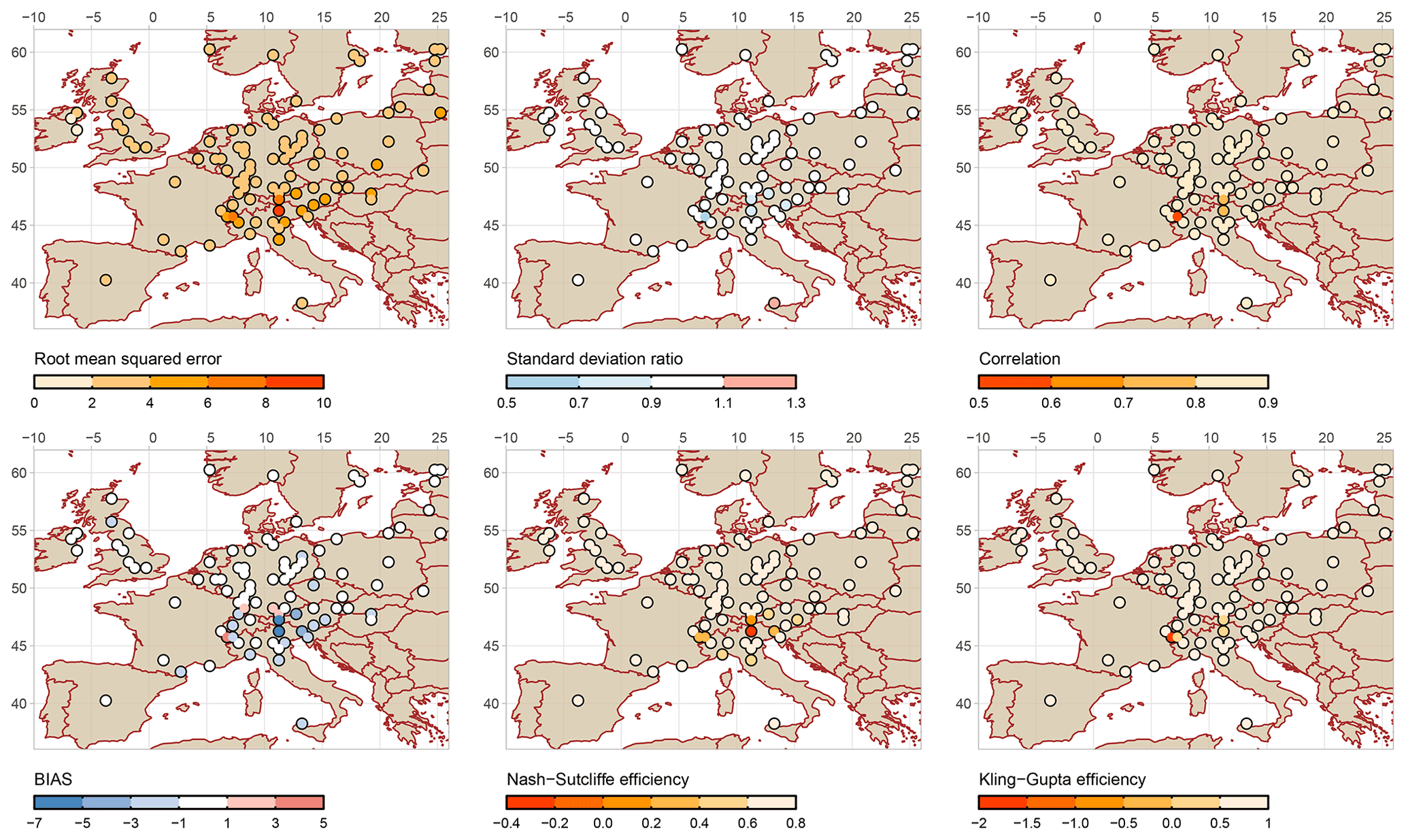
Figure 4Validation of reconstructed temperature (Luterbacher et al., 2004) against GHCN observations.
4.1 Evaluation of reconstructed precipitation and temperature fields
The 500-year annual paleoclimate reconstructions of precipitation (P) and temperature (T) were validated against the GHCN observation data. The map showing the comparison is given in Figs. 3 and 4. The reconstructed data are evaluated against observational P and T across 99 and 94 European sites, respectively. Figure 3 shows that for most of the sites the correlation coefficient (R) of P reconstruction at most of the sites is above 0.5; the relative bias (relBIAS) is between −0.1 and 0.1; KGE and NSE are showing values below 0.5 and 0.6, respectively; the rSD is between 0.7 and 0.9; and RMSE varies between 0 and 150.
The performance of the temperature reconstruction was relatively better, as depicted in Fig. 4. In this case, RMSE between reconstructed and observational T is around 0.2 ∘C, and rSD fluctuates between 0.95 and 1.05, while R is higher than 0.84, and BIAS is less than 0.5 ∘C, except for stations located in the Alps. The NSE and KGE values were above 0.5 at the majority of the stations. Low skill observed at some locations can be explained by the unresolved variability of grid-cell average temperature, especially in regions with complex terrain.
It is worth noting that the large spread of goodness-of-fit (GOF) statistics is mainly due to the outlying values at the grid cells located along the boundary of the domain (i.e. the interface between land and sea/ocean) and high elevations (see also Figs. 3 and 4). In general, reconstructed precipitation exhibits greater differences from observations than temperature. This may be because the proxies considered in the reconstruction rely on different seasons and climate conditions. Additionally, the shortest available instrumental data before the 20th century could encounter certain technical errors, such as problems with instrumental tools, station relocation and dating issues (Dobrovolný et al., 2010). Moreover, other studies (e.g. Ljungqvist et al., 2020) stated that the precipitation series employed for the reconstructions were relatively shorter and more erroneous than the temperature series before the 20th century (Pauling et al., 2006; Harris et al., 2014). Finally, the chosen statistical technique (principal component regression) could also possibly contribute to variance inflation with larger timescales (Pauling et al., 2006).
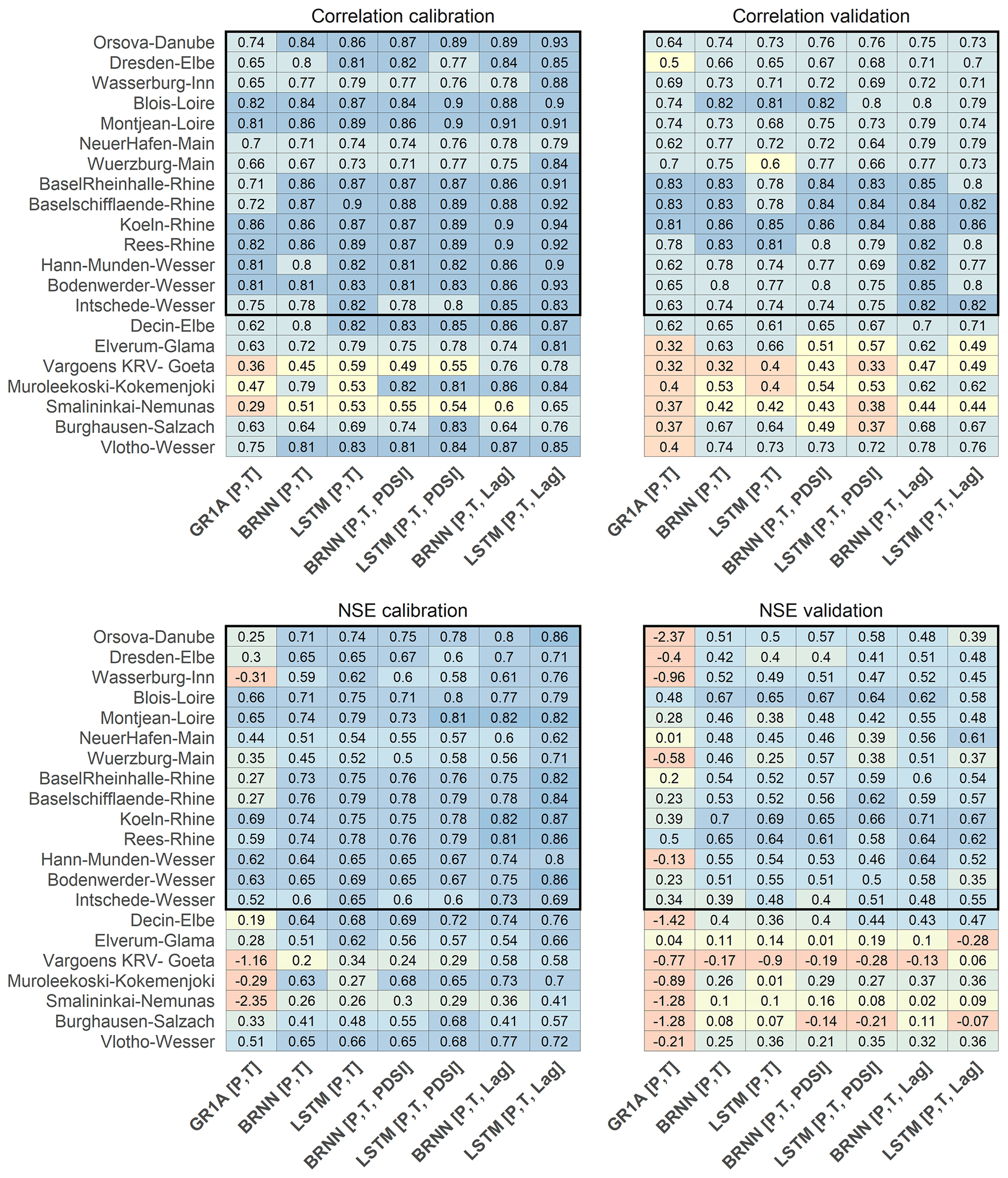
Figure 5The correlation coefficient (top) and NSE (bottom) for calibration (left) and validation (right) of the considered models for 21 study catchments. The vertical axis represents the catchments (station name and river) and the horizontal axis the considered models. The rectangular black frames represent the catchments with NSE > 0.5 over the validation period.
4.2 Assessment of the reconstructed runoff simulations
The GR1A conceptual hydrological model was driven by catchment average P and T and calibrated using observed annual runoff for each catchment separately. The simulated annual runoff series were then compared to the corresponding GRDC observations (for calibration and validation periods), and the results were summarized by means of GOF statistics. As can be seen in Fig. 5, the correlation and NSE statistics for calibration achieve reasonable results at most of the catchments, with a few exceptions (i.e. Kokemenjoki, Goeta, Nemunas and Inn). The catchments with relatively poor skills are located in northern Europe, which is in line with the previous findings by Seiller et al. (2012), who noted that the lumped hydrological models often exhibit larger uncertainties and fail to capture the extreme catchment values (both high and low) in those regions. The low skill for some of the catchments cannot be easily attributed only to bias in reconstructed precipitation and temperature (described in Sect. 4.1) but rather to low station and proxy coverage in some (especially northern) parts of Europe, leading to biased basin-average precipitation and temperature estimate. Another study of Fathi et al. (2019) suggested that the performance of the GR1A model is less efficient than the new Budyko-framework-based SARIMA model in simulating the annual runoff across the Blue Nile and the Danube catchment. This may be due to the simplified nature of the model that does not easily capture the complex relationship between rainfall and runoff variability.
In general, statistical values presented in heat maps (Fig. 5) indicate that the neural network algorithms are more skilled for runoff prediction than the GR1A model. The NSE and R statistics for the BRNN and LSTM models indicate a significant improvement in runoff prediction, as compared to the results obtained through the GR1A model. For instance, for Basel Rheinhalle the NSE increases from 0.27 to 0.73 (BRNN) and 0.75 (LSTM) for calibration and 0.2 to 0.54 (BRNN) and 0.52 (LSTM) for validation. Moreover, including scPDSI from OWDA with reconstructed forcing increases the performance slightly more (NSE 0.76 for calibration and 0.57/0.59 for validation, for BRNN/LSTM, respectively), and considering the lagged forcing results in the best performance (NSE 0.75/0.8 for calibration and 0.6/0.54 for validation, for BRNN/LSTM).
Similarly for all sites, the data-driven methods exhibited a strong correlation with the observed runoff, with the GR1A simulations resulting most frequently in lower correlation values. Other metrics (RMSE, MAE, KGE, rSD and relBIAS) are shown in Figs. S1–S5 in the Supplement. Across many study locations, the combination of reconstructed forcings and their 1-year lag performed the best in terms of rapid convergence (the number of iterations needed) and high accuracy from all input combinations for both data-driven models (BRNN, LSTM). For the validation period, the mean NSE (across all catchments) for the GR1A model is 0.16, for the BRNN it is 0.68 and it improves to 0.73 for the LSTM . In the case of the mean KGE, GR1A yields 0.62, BRNN is 0.73 and LSTM is 0.78.
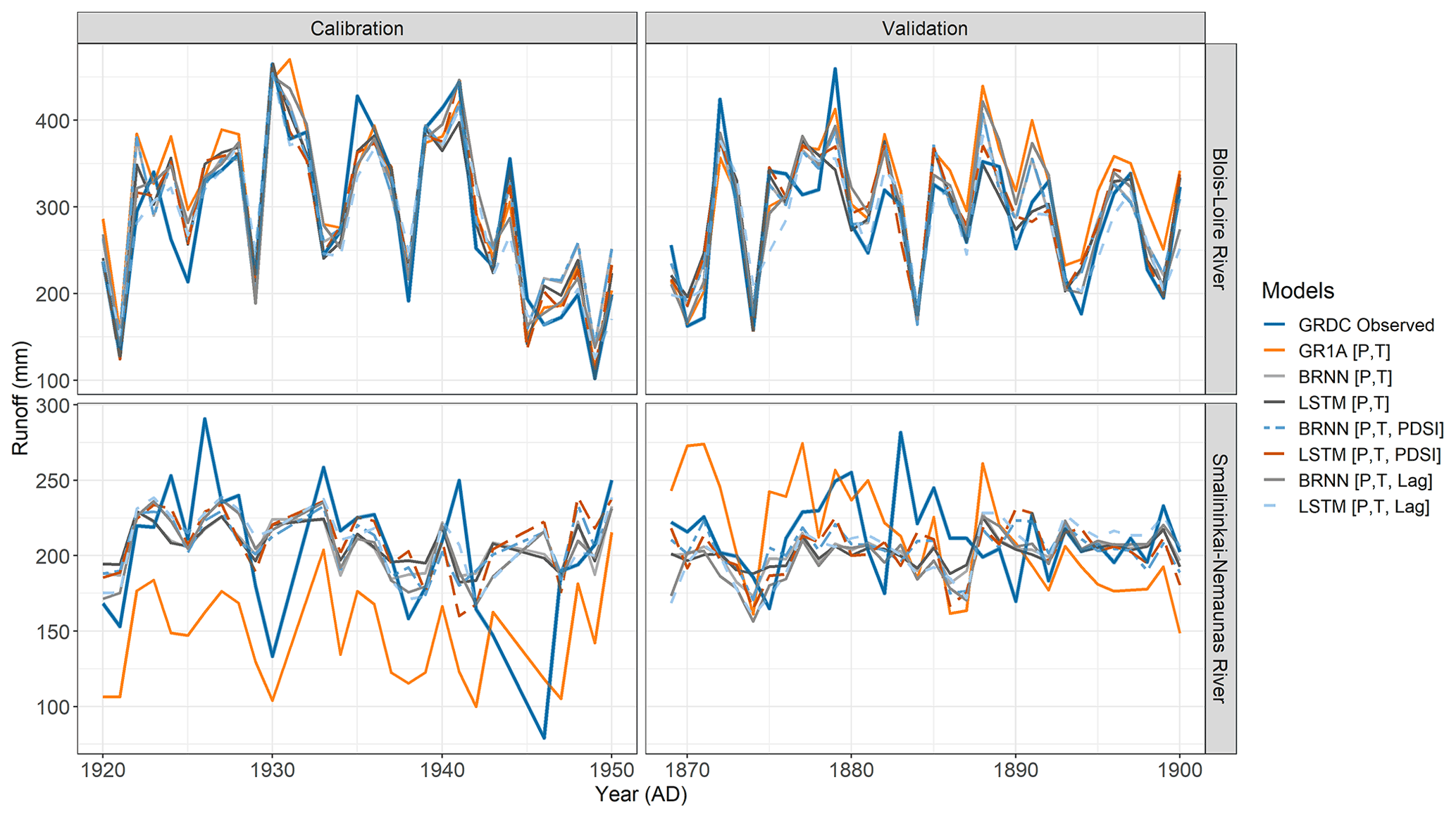
Figure 6Comparison between the models for the station with the best (Blois–Loire River, top) and the worst (Smalininkai–Nemunas River, bottom) model fit.
To further demonstrate the differences between the individual models, we show the simulated runoff series for all models for those catchments with the highest (Blois–Loire) and lowest (Smalininkai–Nemunas) performance in Fig. 6. The performance of the models is comparable during the calibration period for the Loire River. Clearly, all data-driven models are capable of mimicking the observed runoff, while the GR1A model exhibited certain minor deviations, primarily until 1930. In the validation period, the differences between the models are more visible, in particular, for above-average flows. This can be attributed to different generalization skill of individual models. At the beginning of the validation period (1870–1880), all models failed to simulate the high annual flows.
In the case of Nemunas catchment, the GR1A simulation deviates extremely from the observed data and cannot capture the mean flow level. However, the calibration is poor, even for the data-driven models, and does not simulate the year-to-year variability appropriately. Interestingly, for the validation period, the error in the GR1A model decreases. The performance of the data-driven models is similar in validation and calibration periods. Looking at the GOF statistics, the models considering OWDA-based scPDSI or lagged forcings (e.g. Pt−1) perform slightly better in terms of KGE than the other model configurations.
4.3 The annual runoff reconstruction datasets
As a first step, we excluded the catchments that exhibited poor performance in validation (see Fig. 5). As a threshold, we considered validation NSE greater than 0.5 for at least one model, following the approach used by Ayzel et al. (2020). In this step, we excluded 7 catchments (Vlotho–Wesser, Decin–Elbe, Burghausen–Salzach, Smalininkai–Nemunas, Vargoens KRV–Goeta, Elverum–Glama and Muroleekoski–Kokemenjoki) out of 21, ending up with a set of simulations for 14 catchments (highlighted by the rectangular box in Fig. 5).
Secondly, we identified the best candidate models for each of the 14 selected catchments, considering the GOFs based on the validation NSE and R greater than 0.5 and 0.7, respectively. The best model for each catchment was finally selected from those models considering the remaining validation measures (relBIAS, rSD, KGE, RMSE and MAE) as well. Specifically, we picked the models with consistent good validation measures. This choice is partly subjective, and more formal selection should be explored further. On the other hand, the candidate models all performed comparably in most cases.
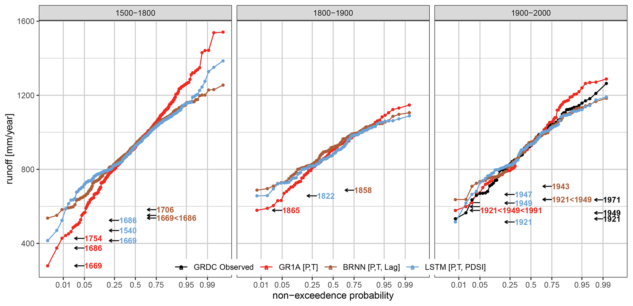
Figure 7Distribution functions for BRNN , LSTM , i.e. the best two models, GR1A [P,T]- and GRDC-observed data for the periods 1500–1800, 1800–1900 and 1900–2000 over the Basel Rheinhalle–Rhine catchment. The values on the horizontal axis are transformed using the “probit” function. The coloured labels indicate the most extreme drought years according to each model.
The resulting selected models are shown in Table 3. The combination of reconstructed forcing with 1-year time lags results in the best performance over nine catchments, of which seven employed the BRNN and the remainder the LSTM model. The LSTM with reconstructed forcing and OWDA-scPDSI was the best in just one case, and the remaining time-series reconstructions were most appropriately simulated with the BRNN [P,T] and BRNN . It should be noted that the differences between the models performing well are small, as noted in Fig. 6 and further demonstrated in Fig. 7. The latter figure compares the cumulative distribution functions of annual runoff for the periods 1500–1800, 1800–1900 and 1900–2000, as simulated by the BRNN and LSTM – the two best-performing models – and the GR1A (the most deviating simulation from the best model) with the distribution of the observed annual runoff for the Basel Rheinhalle–Rhine catchment. For the calibration period (1900–2000) in Fig. 7, the models perform well except the GR1A, which generally overestimated the observed maxima. The cumulative distribution of BRNN- and LSTM-simulated runoff values is very similar for the validation period (1800–1900), except for the top and bottom 5 % in 1500–1800. The GR1A simulation showed significant differences for the entire distribution, thus overestimating/underestimating the maxima/minima. Our finding shows that GR1A simulates a Rhine minimum of 279 mm yr−1 in Basel, whereas the observed minimum in the past century is greater than 532.6 mm yr−1, inferring that the cumulative distribution function (CDF) has significantly lower/higher runoff values between 1500 and 1800 for BRNN and GR1A, whereas LSTM appears to extrapolate less. The difference from the best model can be expressed in terms of KGE – even here, it was evident that the GR1A model deviated considerably (KGE 0.6–0.7), while the LSTM is very similar to the BRNN (KGE 0.92–0.96). The most severe drought year identified by the models in the period 1500–1800 appears to be 1669 and the year 1921 in the past century (1900–2000) (Fig. 7 left and right panels), while for 1800–1900 the models identified either 1865 (GR1A, LSTM) or 1858 (BRNN). Please note that the 1858 low-water mark is available at Laufenburg Pfister et al. (2006) near Basel and was regarded as one of the worst winter droughts in the last 200 years.

Figure 8Reconstruction of runoff series for Köln–Main and Hann. Münden Wesser rivers. The blue line corresponds to the reconstructed series, and the black and red lines represent the observed runoff for the calibration and validation period, respectively.
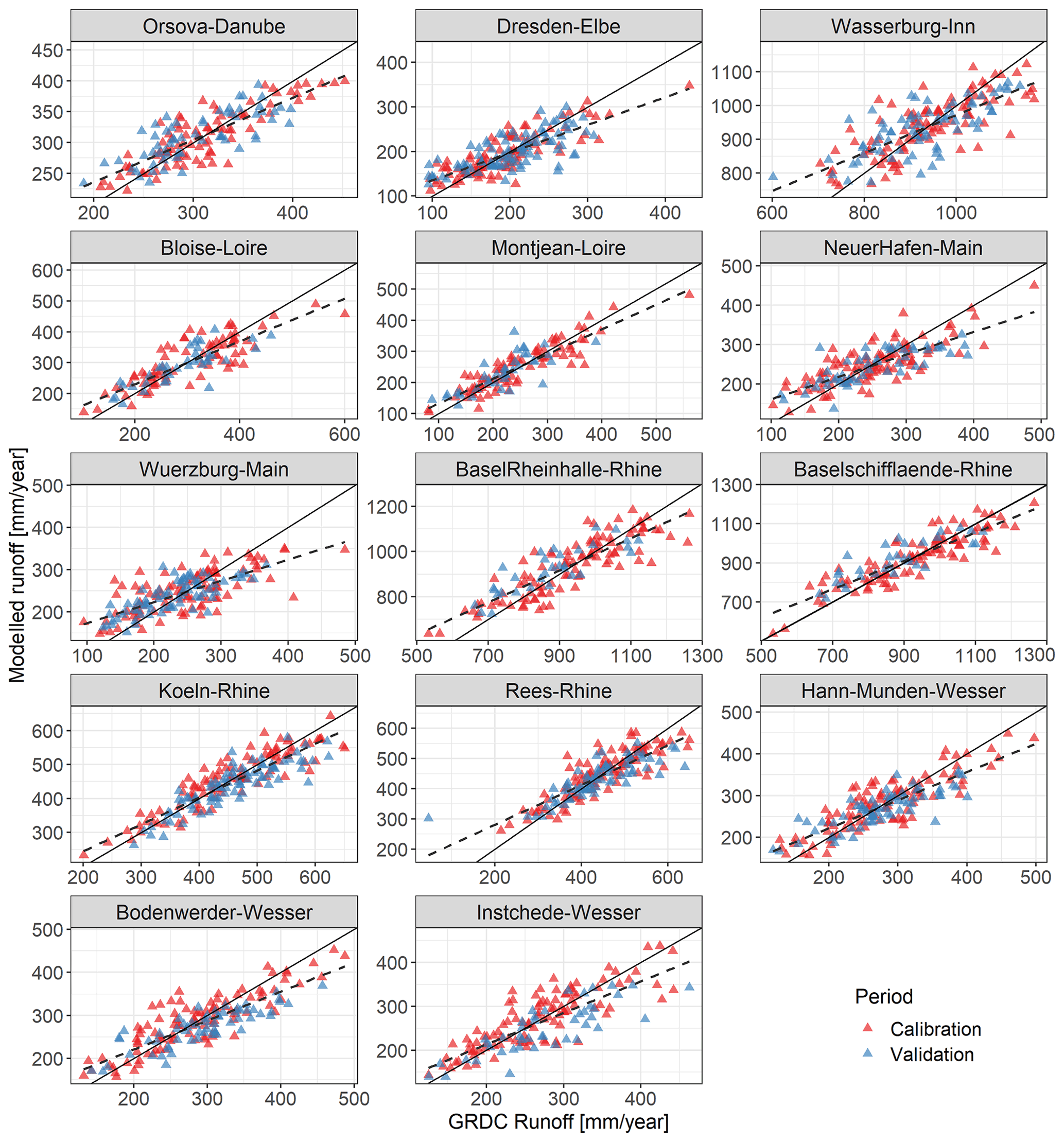
Figure 9Observed and simulated runoff for 14 selected catchments in the calibration and validation periods. The solid line represents the 1:1 relation, and the dashed line corresponds to fitted regression between observed and simulated runoff.
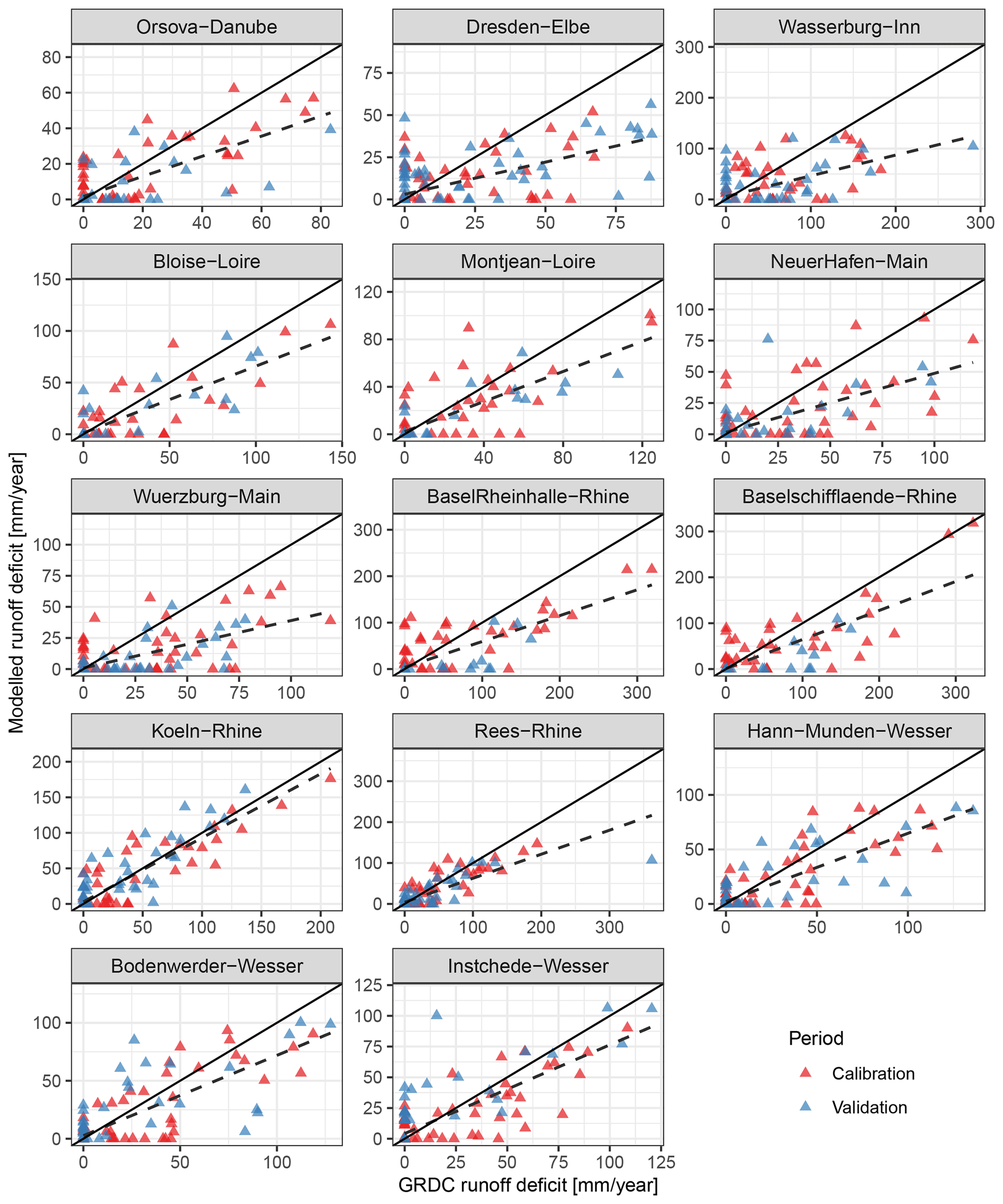
Figure 10The observed and simulated runoff deficit based on the 33rd percentile threshold for 14 selected catchments during the calibration and validation period. The solid line represents the 1:1 relation, and the dashed line corresponds to fitted regression between observed and simulated runoff.
The resulting 14 annual runoff reconstructions are available at https://doi.org/10.6084/m9.figshare.15178107 and are shown in Figs. S6–S8 in the Supplement. As an example, we present only two runoff reconstructions here (Fig. 8). As an additional validation for the reconstructed series, we inspected the scatter plots of the observed and reconstructed runoff (Fig. 9). The simulated series are generally consistent with the observed runoff, especially for the Montjean–Loire, Köln–Rhine and Basel Schifflaende–Rhine catchments, which exhibit the best relationship between the observed and the simulated runoff.
Finally, to check the consistency of our reconstructed dataset, we compared the skill of our simulation with respect to the GRDC runoff observation and the GSWP3-forced GRUN monthly runoff (Ghiggi et al., 2019) datasets. The gridded GRUN datasets were averaged over the respective catchments to enable comparison (Figs. S9 and S10 in the Supplement). Our reconstruction outperforms GRUN data in terms of RMSE, MAE, relBIAS and NSE across the majority of the catchments, while the correlation (reproduction of interannual dynamics) to GRDC runoff is slightly higher for GRUN compared to our reconstruction. The variability, which our data-driven models underestimate (on average by 16.5 %), is overestimated by GRUN (on average by 17.2 %). Since the correlation compensates for the relBIAS, the KGE for our reconstruction and GRUN is comparable. This suggests that GRUN could be used for data-driven model training, provided at least some information on flow characteristics is available in the catchment.
Table 3Selection of best model for runoff in individual catchments.

4.4 Identification of low flows, significant hydrological drought events and trends
In the final step of the analysis, we compared the droughts identified in the reconstructions with the GRDC-observed series (Fig. 10). The agreement between the simulated and observed runoff deficit is lower compared to the annual runoff time series. For most of the stations, the simulated deficit is lower than the corresponding observed estimates. This suggests that the reconstructed precipitation and temperature fields do not represent the inter-annual variability correctly. Despite a widespread issue with the representation of inter-annual persistence, Fig. 10 shows that the runoff deficits are simulated reasonably well for the Rees–Rhine and Köln–Rhine catchments.
Table 4Simulated runoff droughts since 1500. Years in bold indicate extreme droughts below 5 % quantile.
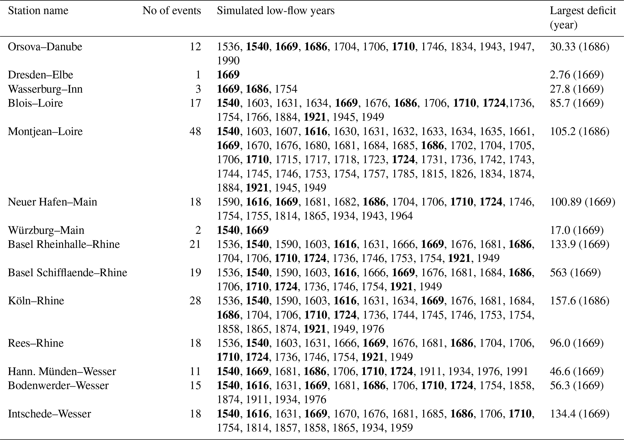
Furthermore, we contrasted reconstructed drought patterns over the last 500 years with data available from documentary evidence and other sources. In the case of extreme droughts, we considered the q0.05 threshold before 2000 CE. Low-flow analysis since 1500 and the large deficit values for catchments (below 5th percentile) are shown in Table 4. In the 16th century, the years 1536, 1540 and 1590 are associated with significant runoff deficits. The event of 1540 has already been reported (Brázdil et al., 2013; Cook et al., 2015; Brázdil et al., 2019) as the worst event of the 16th century and more severe in terms of changing hydrologic conditions. In 1540, almost 90 % of the Rhine and Elbe River catchments (Basel and Cologne) experienced low yearly discharge, which ranked as the greatest low flows in the last 5 centuries (Leggewie and Mauelshagen, 2018). The seasonal precipitation was also deficient and was evident primarily in central Europe and England (Dobrovolný et al., 2010). Wetter and Pfister (2013) stated that the spring and summer of 1540 were likely to have been warmer than the comparable period during the 2003 drought. The simulation shows that the drought during 1540 was evident in most study catchments, such as the Rhine, Main, Wesser, Loire and Danube, except Wasserburg–Inn.
In the 17th century, the years 1603, 1616, 1631, 1666, 1669, 1676, 1681, 1684 and 1686 were simulated as exceptionally low-flow years. Furthermore, two events (1669 and 1686) were associated with the largest water deficit across several study catchments. Basel Schifflaende–Rhine catchment is a good example of this, which appears to have experienced an extreme runoff deficit during 1669. In the Köln–Rhine catchment, 26 remarkable droughts have been captured over the past 500 years, and the year 1686 reached the largest runoff deficit (156 mm yr−1). The 1616 is considered the driest year of the 17th century, the so-called “drought of the century” (Brázdil et al., 2013), which significantly impacted the major rivers in Europe (e.g. Rhine, Main and Wesser). Brázdil et al. (2018) identified three unusual drought periods (1540, 1616 and 1718–19) over the Czech lands, highlighting the 1616 drought, which caused widespread famine, dried up the Elbe river watershed and altered the climate of neighbouring nations (Switzerland and Germany). The hunger stone of the Elbe River also revealed the exceptionally dry year of 1616 (Brázdil et al., 2013). During the 18th century, a similar level of runoff deficit was simulated in the years 1706 and 1719.
During the 19th century, the years 1863, 1864, 1874, 1893 and 1899 were recognized as drought years in all catchments, while in the 20th century, the driest periods occurred in 1921, 1934, 1949 and 1976. The 1921 drought in the Blois–Loire, Rees–Rhine, Köln–Rhine, Orsova–Danube, Basel Rheinhalle–Rhine and Basel Schifflaende–Rhine catchments was ranked as the most exceptional drought in the 20th century. Three catchments (Basel Rheinhalle–Rhine, Basel Schifflaende–Rhine and Blois–Loire) exhibited a large runoff deficit during the year 1921. A noticeable increase in temperature was experienced across Europe, and certain areas were notably affected by a heatwave in July of that year. The majority of central Europe, southern England and Italy were affected by this drought, where the rainfall was found to have decreased around 50 % to 60 % relative to the average (Bonacina, 1923; Cook et al., 2015). The precipitation totals were recorded as the lowest since 1774, and the year was also ranked top (in terms of deficit rainfall) in the Great Alpine region (Haslinger and Blöschl, 2017), where the rainfall deficit began in winter 1920/21 and lasted until autumn 1921. Also reported in newspapers, the Rhine River (Switzerland), Molesey Weir on the Thames River (United Kingdom) and Loire River (France) all had low river flows in 1921 (Van der Schrier et al., 2021). Monthly runoff anomalies analysed from the GRUN dataset (Ghiggi et al., 2019) show that August 1976 was the fifth driest month between 1900 and 2014, in agreement with some of our catchment reconstructions signalling the 1976 as a yearly drought in the Köln–Rhine, Hann. Münden–Wesser and Bodenwerder–Wesser.
In summary, the reconstructed annual runoff corresponded well to the majority of extreme drought years (e.g. 1540, 1616, 1669, 1710, 1724 and 1921, as highlighted in Table 4) and previously demonstrated in the OWDA-based PDSI tree-ring reconstructions and previous works (Dobrovolný et al., 2010; Brázdil et al., 2013; Wetter and Pfister, 2013; Cook et al., 2015; Markonis et al., 2018). It is important to note that the presented runoff reconstructions might have missed notably documented dry events, e.g. 1894 (Brodie, 1894), which was associated with unprecedented low levels of rainfall and excessive temperature rises in the south of England, the British Isles and other European regions (Brodie, 1894; Cook et al., 2015; Hanel et al., 2018).
Finally, we assessed the linear trends in the decadal runoff series for several time periods. The reconstructed annual runoff for 1500–2000 for each catchment was first aggregated to 10-year averages and divided by the mean annual runoff. The resulting series are shown in Fig. A2. Although significant negative trends were found for all catchments except for one considering the whole 1500–2000 period, the signal is not clearly linear. Instead, for a number of catchments, there is a period of sustained above-average (Orsova–Danube and Dresden–Elbe) or below-average (Blois and Montjean Loire) annual runoff during approx. 1600–1800, while for the rest, the persistence is weaker, although a low runoff signal is still visible (Basel Rheinhalle, Basel Schifflaende and Köln Rhine). When only the last 50 years is considered, the trends are significantly negative (positive) for seven (two) catchments, with the rest being insignificant.
The annual runoff reconstructions were prepared using the defined dataset and can be accessed on the public repository Figshare (https://doi.org/10.6084/m9.figshare.15178107, Sadaf et al., 2021). The reconstructed data of precipitation and temperature can be downloaded at https://www.ncdc.noaa.gov/data-access/paleoclimatology-data (last access: 20 Feburary 2020). The monthly global historical climatological network (GHCN) data can be accessed via the link https://www1.ncdc.noaa.gov/pub/data/ghcn/ (last access: 12 May 2019). The data repositories of GRDC runoff are accessible to the public at https://www.bafg.de/GRDC/EN/Home/homepage_node.html (last access: 24 November 2016). All analyses and visualizations were done using R.
In this study, hydrological (GR1A) and two data-driven (BRNN and LSTM) models were used to reconstruct the annual runoff during the period 1500–2000, considering various input fields. After comprehensive validation of the simulated series, this work provides annual runoff time series for 14 catchments across Europe. The presented dataset can be used to investigate annual drought duration and severity. The main findings can be summarized as follows:
-
Data-driven methods have proven to be helpful for annual runoff simulations, even when there is high uncertainty in the forcing meteorological data. This contrasts with a conceptual lumped hydrological model, which would require bias correction before hydrological simulation.
-
There is no significant difference between the BRNN- and LSTM-simulated annual runoff, neither in terms of the individual values, nor in relation to the validation metrics.
-
Validation skill metrics suggest that for annual runoff prediction, it is beneficial to consider data-driven models that explicitly account for serial dependence, either through input data (e.g. time-lagged input fields) or directly in the model structure (e.g. LSTM networks).
-
The droughts identified in the reconstructed series correlate well with significant documented events (such as 1540, 1616, 1669, 1710, 1724 and 1921).
The reconstructed annual runoff relies heavily on the consistency of underlying reconstructed precipitation (Pauling et al., 2006) and temperature (Luterbacher et al., 2004) forcing fields. Unfortunately, those cannot be fully verified directly, due to the lack of sufficient long-term observational datasets. With the limited information provided by the GHCN station, we identified several notable deficiencies in the reconstructed forcings, in particular, underestimation of the variance in precipitation reconstruction. Moreover, proxy records that were used for the derivation of precipitation and temperature input fields are spatially heterogeneous, with some regions being better represented than others. This inevitably leads to poor performance over the latter. The skill of precipitation and temperature reconstructions across the selected catchments to derive annual runoff is still fairly good. In addition, the data-driven methods that were used in the paper were capable of removing systematic bias. We cannot be sure, though, that the link between reconstructed forcing and annual runoff is stationary when going back in time. Moreover, when the number of natural proxies included in the derivation of the forcing dataset decreases, the uncertainty increases. The reconstructed data should, therefore, always be considered with caution. Finally, since the runoff reconstruction is annual, dry summers can be compensated for by wet winters masking years with sub-annual dry periods. However, this should be regarded as a resolution- not methodology-related problem. Future research could consider further improvements of the simulations, e.g. by training a meta-model combining the runoff simulations from several fitted models. In addition, since interest is not often focused on the runoff series but on some other indicator (such as PDSI or deficit volume in the case of drought), it is also possible to simulate the drought indices directly, considering either the precipitation and temperature input fields or the simulated runoff. Finally, discrete classifiers (Kolachian and Saghafian, 2021) could also be used to simulate the drought (or water level) classes directly.
A1 Goodness-of-fit assessment
We used several statistical indicators to assess the skill of annual runoff reconstruction. In following definitions, p and o refer to the predicted and observed series, respectively, and i to year.
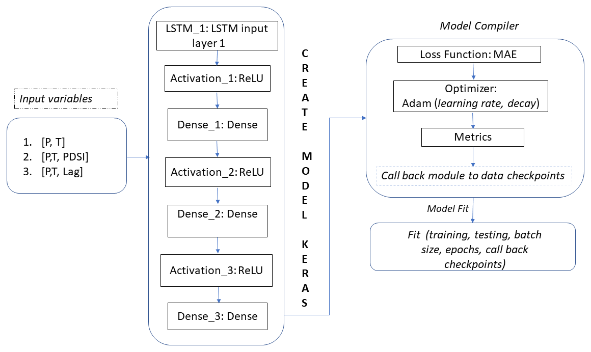
Figure A1Structure of LSTM neural network model in a Keras environment for runoff predictions.
Table A1Structure and hyperparameters of two data-driven models (BRNN and LSTM) for runoff predictions.

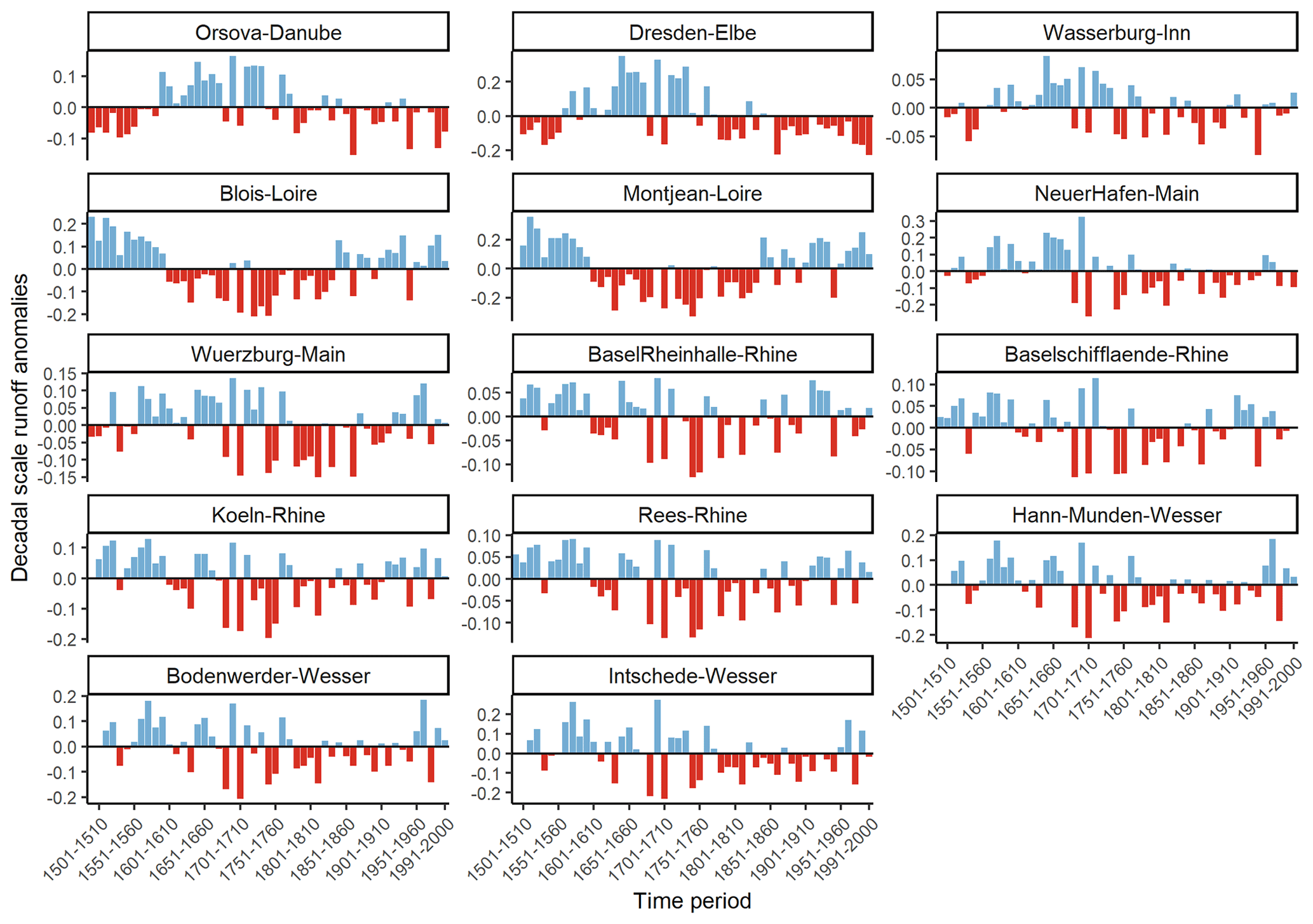
Figure A2Decadal fluctuation of runoff anomalies in selected catchments over the past 500 years.
The standard deviation (SD) ratio (rSD; Ghiggi et al., 2021) is defined as
The variability is underestimated when the value is less than 1 and overestimated when the value is greater than 1.
The root mean square error (RMSE; see, for example, Legates and McCabe, 1999)
and mean absolute error (MAE; see e.g. Legates and McCabe, 1999)
measure how well predictions fit the observations. MAE and RMSE values can range from zero to infinity, with the former value indicating a perfect fit.
Pearson's correlation coefficient (R) is defined as
The Nash–Sutcliffe efficiency (NSE; Nash and Sutcliffe, 1970),
is alternatively referred to as model efficiency. NSE = 1 corresponds to a perfect match between predicted and observed data, while a value less than 0 indicates that model predictions are on average less accurate than using the long-term mean of the observed time series .
Systematic errors can be detected using the absolute bias (BIAS)
or relative bias (relBIAS)
which has an ideal value of 0. Positive bias values indicate that the model prediction overestimates observations, whereas negative values indicate underestimated model predictions.
The Kling–Gupta efficiency index (KGE; Gupta et al., 2009)
is calculated using three primary components, R, rSD and relBIAS, as defined above. relBIAS has a zero ideal value, while rSD and R have an ideal value of 1.
A2 Long short-term memory (LSTM)
To build the LSTM model, we use the Keras environment (Arnold, 2017) with its high-level application programming interface (API) for neural networks and Tensorflow (Abadi et al., 2016). Fig. A1 represents the structure of the LSTM neural model for the rainfall runoff relationship in several catchments. We design our network by stacking one LSTM and two dense layers on top of one other. As shown in Fig. A1, the model configured four distinct input combinations, each of which was normalized to [0,1] in the training and testing phases. The model parameters choose different batch shapes, units (similar as neurons) and epochs as described in Table A1. The model considers the rectified linear unit (ReLU), using component wise multiplication and defining the dropout parameter as 0.1. According to Kingma and Ba (2014), the optimization algorithm plays a significant role in the algorithm's convergence and optimization. For this reason, Adam's optimizer is considered, as it performs stochastic gradient descent (SGD) more efficiently using the backpropagation algorithm. During compilation, the learning rate is set to 0.001 or 0.002, and the mean square error (MSE) is used to measure model accuracy. In addition, the mean absolute error (MAE) is used as an objective to minimize residues and achieve optimum value. Model checkpoints are used to save the model having minimum loss during the training with minimum loss and better accuracy.
A3 Bayesian regularized neural network (BRNN)
BRNN is a probabilistic technique for handling non-linear problems. Using the caret package, the model “brnn” was designed to work with a two-layer network as described by MacKay (1992) and Foresee and Hagan (1997). BRNN uses the Nguyen and Widrow algorithm to assign initial weights and the Gauss–Newton algorithm to optimize. Model is first trained on the training dataset, and its performance is checked by making a prediction on the testing dataset.
While selecting a model for train control, a simple boot resampling strategy was applied to evaluate performance. We tested the proposed model's predictive ability using a random bootstrap generator, with 75 % of the observations in the training set and 25 % in the testing set. RMSE was utilized as a loss function to compile and verify the model's accuracy. The model was fitted with 20 neurons, one hidden layer and implemented activation function . After compilation, the train function automatically selected the best model with the smallest RMSE as the final model.
The supplement related to this article is available online at: https://doi.org/10.5194/essd-14-4035-2022-supplement.
The study was initially designed by RK, MH and YM. Algorithms are coded with the assistance of YM, US and MH. Datasets were collected by MRVG and SN. The research was carried out by SN, MS and MH, who also wrote the paper. OR and RK both helped to revise the manuscript.
The contact author has declared that none of the authors has any competing interests.
Publisher's note: Copernicus Publications remains neutral with regard to jurisdictional claims in published maps and institutional affiliations.
This work was carried out within the bilateral project XEROS (eXtreme EuRopean drOughtS: multimodel synthesis of past, present and future events). We thank the Global Runoff Data Centre (GRDC) for providing the observed runoff data. We would also like to thank the editor, Christof Lorenz (KIT, Germany), Gionata Ghiggi (EPFL, Switzerland) and the anonymous reviewers for their insightful remarks, which improved the overall quality of the article.
This research has been supported by the Grantová Agentura České Republiky (grant no. 1924089J), the Deutsche Forschungsgemeinschaft (grant no. RA 3235/11) and the Fakulta Životního Prostředí, Česká Zemědělská Univerzita v Praze (grant no. 2020B0018).
This paper was edited by Christof Lorenz and reviewed by Gionata Ghiggi and two anonymous referees.
Abadi, M., Barham, P., Chen, J., Chen, Z., Davis, A., Dean, J., Devin, M., Ghemawat, S., Irving, G., Isard, M., Kudlur, M., Levenberg, J., Monga, R., Moorea, S., Murray, D. G., Steiner, B., Tucker, P., Vasudevan, V., Warden, P., Wicke, M., Yu, Y., Zheng, X., and Google brain: Tensorflow: A system for large-scale machine learning, in: 12th {USENIX} symposium on operating systems design and implementation ({OSDI} 16, 2–4 November 2016, Savannah, GA, USA, pp. 265–283, 2016. a, b
Armstrong, M. S., Kiem, A. S., and Vance, T. R.: Comparing instrumental, palaeoclimate, and projected rainfall data: Implications for water resources management and hydrological modelling, Journal of Hydrology: Regional Studies, 31, 100728, https://doi.org/10.1016/j.ejrh.2020.100728, 2020. a
Arnold, T. B.: kerasR: R interface to the keras deep learning library, Journal of Open Source Software, 2, 296, https://doi.org/10.21105/joss.00296, 2017. a, b
Ayzel, G., Kurochkina, L., and Zhuravlev, S.: The influence of regional hydrometric data incorporation on the accuracy of gridded reconstruction of monthly runoff, Hydrol. Sci. J., 0, https://doi.org/10.1080/02626667.2020.1762886, 1–12, 2020. a
Boch, R. and Spötl, C.: Reconstructing palaeoprecipitation from an active cave flowstone, J. Quaternary Sci., 26, 675–687, 2011. a
Bonacina, L.: The European drought of 1921, Nature, 112, 488–489, 1923. a
Brázdil, R. and Dobrovolný, P.: Historical climate in Central Europe during the last 500 years, The Polish Climate in the European Context: An Historical Overview, Springer, Dordrecht, the Netherlands, p. 41, 2009. a
Brázdil, R., Dobrovolný, P., Trnka, M., Kotyza, O., Řezníčková, L., Valášek, H., Zahradníček, P., and Štěpánek, P.: Droughts in the Czech Lands, 1090–2012 AD, Clim. Past, 9, 1985–2002, https://doi.org/10.5194/cp-9-1985-2013, 2013. a, b, c, d
Brázdil, R., Kiss, A., Luterbacher, J., Nash, D. J., and Řezníčková, L.: Documentary data and the study of past droughts: a global state of the art, Clim. Past, 14, 1915–1960, https://doi.org/10.5194/cp-14-1915-2018, 2018. a, b
Brázdil, R., Demarée, G. R., Kiss, A., Dobrovolný, P., Chromá, K., Trnka, M., Dolák, L., Řezníčková, L., Zahradníček, P., Limanowka, D., and Jourdain, S.: The extreme drought of 1842 in Europe as described by both documentary data and instrumental measurements, Clim. Past, 15, 1861–1884, https://doi.org/10.5194/cp-15-1861-2019, 2019. a
Brodie, F. J.: The great drought of 1893, and its attendant meteorological phenomena, Q. J. Roy. Meteor. Soc., 20, 1–30, 1894. a, b
Büntgen, U., Frank, D. C., Nievergelt, D., and Esper, J.: Summer temperature variations in the European Alps, AD 755–2004, J. Climate, 19, 5606–5623, 2006. a
Büntgen, U., Franke, J., Frank, D., Wilson, R., González-Rouco, F., and Esper, J.: Assessing the spatial signature of European climate reconstructions, Clim. Res., 41, 125–130, 2010. a
Caillouet, L., Vidal, J.-P., Sauquet, E., Devers, A., and Graff, B.: Ensemble reconstruction of spatio-temporal extreme low-flow events in France since 1871, Hydrol. Earth Syst. Sci., 21, 2923–2951, https://doi.org/10.5194/hess-21-2923-2017, 2017. a
Casas-Gómez, P., Sánchez-Salguero, R., Ribera, P., and Linares, J. C.: Contrasting Signals of the Westerly Index and North Atlantic Oscillation over the Drought Sensitivity of Tree-Ring Chronologies from the Mediterranean Basin, Atmosphere, 11, 644, https://doi.org/10.3390/atmos11060644, 2020. a
Casty, C., Wanner, H., Luterbacher, J., Esper, J., and Böhm, R.: Temperature and precipitation variability in the European Alps since 1500, Int. J. Climatol., 25, 1855–1880, 2005. a
Chen, X., Huang, J., Han, Z., Gao, H., Liu, M., Li, Z., Liu, X., Li, Q., Qi, H., and Huang, Y.: The importance of short lag-time in the runoff forecasting model based on long short-term memory, J. Hydrol., 589, 125359, https://doi.org/10.1016/j.jhydrol.2020.125359, 2020. a
Contreras, P., Orellana-Alvear, J., Muñoz, P., Bendix, J., and Célleri, R.: Influence of Random Forest Hyperparameterization on Short-Term Runoff Forecasting in an Andean Mountain Catchment, Atmosphere, 12, 238, https://doi.org/10.3390/atmos12020238, 2021. a
Cook, E. R., Seager, R., Kushnir, Y., Briffa, K. R., Büntgen, U., Frank, D., Krusic, P. J., Tegel, W., van der Schrier, G., Andreu-Hayles, L., Baillie, M., Baittinger, C., Bleicher, N., Bonde, N., Brown, D., Carrer, M., Cooper, R., Čufar, K., Dittmar, C., Esper, J., Griggs, C., Gunnarson, B., Günther, B., Gutierrez, E., Haneca, K., Helama, S., Herzig, F., Heussner, K. U., Hofmann, J., Janda, P., Kontic, R., Köse, N., Kyncl, T., Levanič, T., Linderholm, H., Manning, S., Melvin, T. M., Miles, D., Neuwirth, B., Nicolussi, K., Nola, P., Panayotov, M., Popa, I., Rothe, A., Seftigen, K., Seim, A., Svarva, H., Svoboda, M., Thun, T., Timonen, M., Touchan, R., Trotsiuk, V., Trouet, V., Walder, F., Ważny, T., Wilson, R., and Zang, C.: Old World megadroughts and pluvials during the Common Era, Science Advances, 1, e1500561, https://doi.org/10.1126/sciadv.1500561, 2015. a, b, c, d, e, f, g, h, i, j, k
Coron, L., Thirel, G., Delaigue, O., Perrin, C., and Andréassian, V.: The suite of lumped GR hydrological models in an R package, Environ. Modell. Softw., 94, 166–171, 2017. a
Dobrovolný, P., Moberg, A., Brázdil, R., Pfister, C., Glaser, R., Wilson, R., van Engelen, A., Limanówka, D., Kiss, A., Halíčková, M., Macková, J., Riemann, D., Luterbacher, J., and Böhm, R.: Monthly, seasonal and annual temperature reconstructions for Central Europe derived from documentary evidence and instrumental records since AD 1500, Climatic Change, 101, 69–107, 2010. a, b, c, d, e
Emile-Geay, J., McKay, N. P., Kaufman, D. S., Von Gunten, L., Wang, J., Anchukaitis, K. J., Abram, N. J., Addison, J. A., Curran, M. A., Evans, M. N., Henley, B. J., Hao, Z., Martrat, B., McGregor, H. V., Neukom, R., Pederson, G. T., Stenni, B., Thirumalai, K., Werner, J. P., Xu, C., Divine, D. V., Dixon, B. C., Gergis, J., Mundo, I. A., Nakatsuka, T., Phipps, S. J., Routson, C. C., Steig, E. J., Tierney, J. E., Tyler, J. J., Allen, K. J., Bertler, N. A. N., Björklund, J., Chase, B. M., Chen, M.-T., Cook, E., de Jong, R., DeLong, K. L., Dixon, D. A., Ekaykin, A. A., Ersek, V., Filipsson, H. L., Francus, P., Freund, M. B., Frezzotti, M., Gaire, N. P., Gajewski, K., Ge, Q., Goosse, H., Gornostaeva, A., Grosjean, M., Horiuchi, K., Hormes, A., Husum, K., Isaksson, E., Kandasamy, S., Kawamura, K., Kilbourne, K. H., Koç, N., Leduc, G., Linderholm, H. W., Lorrey, A. M., Mikhalenko, V., Mortyn, P. G., Motoyama, H., Moy, A. D., Mulvaney, R., Munz, P. M., Nash, D. J., Oerter, H., Opel, T., Orsi, A. J., Ovchinnikov, D. V., Porter, T. J., Roop, H. A., Saenger, C., Sano, M., Sauchyn, D., Saunders, K. M., Seidenkrantz, M.-S., Severi, M., Shao, X., Sicre, M.-A., Sigl, M., Sinclair, K., St. George, S., St. Jacques, J.-M., Thamban, M., Kuwar Thapa, U., Thomas, E. R., Turney, C., Uemura, R., Viau, A. E., Vladimirova, D. O., Wahl, E. R., White, J. W. C., Yu, Z., Zinke, J., and PAGES2k Consortium: A global multiproxy database for temperature reconstructions of the Common Era, Scientific Data, 4, 170088, https://doi.org/10.1038/sdata.2017.88, 2017. a
Fathi, M. M., Awadallah, A. G., Abdelbaki, A. M., and Haggag, M.: A new Budyko framework extension using time series SARIMAX model, J. Hydrol., 570, 827–838, 2019. a
Fekete, B. M., Vörösmarty, C. J., and Grabs, W.: Global, composite runoff fields based on observed river discharge and simulated water balances, Tech. Rep. 22, Global Runoff Data Centre, Koblenz, Germany, 1999. a
Foresee, F. D. and Hagan, M. T.: Gauss-Newton approximation to Bayesian learning, in: Proceedings of international conference on neural networks (ICNN'97), vol. 3, pp. 1930–1935, IEEE, Houston, TX, USA, 1997. a
Ghiggi, G., Humphrey, V., Seneviratne, S. I., and Gudmundsson, L.: GRUN: an observation-based global gridded runoff dataset from 1902 to 2014, Earth Syst. Sci. Data, 11, 1655–1674, https://doi.org/10.5194/essd-11-1655-2019, 2019. a, b, c
Ghiggi, G., Humphrey, V., Seneviratne, S., and Gudmundsson, L.: G-RUN ENSEMBLE: A Multi-Forcing Observation-Based Global Runoff Reanalysis, Water Resour. Res., 57, e2020WR028787, https://doi.org/10.1029/2020WR028787, 2021. a
Gupta, H. V., Kling, H., Yilmaz, K. K., and Martinez, G. F.: Decomposition of the mean squared error and NSE performance criteria: Implications for improving hydrological modelling, J. Hydrol., 377, 80–91, https://doi.org/10.1016/j.jhydrol.2009.08.003, 2009. a
Hanel, M., Rakovec, O., Markonis, Y., Máca, P., Samaniego, L., Kyselỳ, J., and Kumar, R.: Revisiting the recent European droughts from a long-term perspective, Scientific Reports, 8, 1–11, 2018. a, b, c, d
Hansson, D., Eriksson, C., Omstedt, A., and Chen, D.: Reconstruction of river runoff to the Baltic Sea, AD 1500–1995, Int. J. Climatol., 31, 696–703, 2011. a, b
Harris, I., Jones, P. D., Osborn, T. J., and Lister, D. H.: Updated high-resolution grids of monthly climatic observations–the CRU TS3.10 Dataset, Int. J. Climatol., 34, 623–642, 2014. a
Haslinger, K. and Blöschl, G.: Space-time patterns of meteorological drought events in the European Greater Alpine Region over the past 210 years, Water Resour. Res., 53, 9807–9823, 2017. a
Hochreiter, S. and Schmidhuber, J.: Long short-term memory, Neural Comput., 9, 1735–1780, 1997. a
Hu, C., Wu, Q., Li, H., Jian, S., Li, N., and Lou, Z.: Deep learning with a long short-term memory networks approach for rainfall-runoff simulation, Water, 10, 1543, https://doi.org/10.3390/w10111543, 2018. a, b
Im, S., Kim, H., Kim, C., and Jang, C.: Assessing the impacts of land use changes on watershed hydrology using MIKE SHE, Environ. Geol., 57, 231, https://doi.org/10.1007/s00254-008-1303-3, 2009. a
Ionita, M., Tallaksen, L. M., Kingston, D. G., Stagge, J. H., Laaha, G., Van Lanen, H. A. J., Scholz, P., Chelcea, S. M., and Haslinger, K.: The European 2015 drought from a climatological perspective, Hydrol. Earth Syst. Sci., 21, 1397–1419, https://doi.org/10.5194/hess-21-1397-2017, 2017. a
Jeong, J., Barichivich, J., Peylin, P., Haverd, V., McGrath, M. J., Vuichard, N., Evans, M. N., Babst, F., and Luyssaert, S.: Using the International Tree-Ring Data Bank (ITRDB) records as century-long benchmarks for global land-surface models, Geosci. Model Dev., 14, 5891–5913, https://doi.org/10.5194/gmd-14-5891-2021, 2021. a
Ji, Y., Dong, H.-T., Xing, Z.-X., Sun, M.-X., Fu, Q., and Liu, D.: Application of the decomposition-prediction-reconstruction framework to medium-and long-term runoff forecasting, Water Supply, 21, 696–709, 2021. a
Kingma, D. P. and Ba, J.: Adam: A method for stochastic optimization, arXiv [preprint], arXiv:1412.6980, 2014. a
Kolachian, R. and Saghafian, B.: Hydrological drought class early warning using support vector machines and rough sets, Environ. Earth Sci., 80, 1–15, 2021. a
Kratzert, F., Klotz, D., Brenner, C., Schulz, K., and Herrnegger, M.: Rainfall–runoff modelling using Long Short-Term Memory (LSTM) networks, Hydrol. Earth Syst. Sci., 22, 6005–6022, https://doi.org/10.5194/hess-22-6005-2018, 2018. a
Kress, A., Saurer, M., Siegwolf, R. T., Frank, D. C., Esper, J., and Bugmann, H.: A 350 year drought reconstruction from Alpine tree ring stable isotopes, Global Biogeochem. Cy., 24, 1–16, https://doi.org/10.1029/2009GB003613, 2010. a
Kress, A., Hangartner, S., Bugmann, H., Büntgen, U., Frank, D. C., Leuenberger, M., Siegwolf, R. T., and Saurer, M.: Swiss tree rings reveal warm and wet summers during medieval times, Geophys. Res. Lett., 41, 1732–1737, 2014. a, b
Krysanova, V., Vetter, T., and Hattermann, F.: Detection of change in drought frequency in the Elbe basin: comparison of three methods, Hydrol. Sci. J., 53, 519–537, 2008. a
Kuhn, M.: Caret: classification and regression training, Astrophysics Source Code Library, https://ui.adsabs.harvard.edu/abs/2015ascl.soft05003K (last access: 21 December 2021), pp. ascl–1505, 2015. a
Kwak, J., Lee, J., Jung, J., and Kim, H. S.: Case Study: Reconstruction of Runoff Series of Hydrological Stations in the Nakdong River, Korea, Water, 12, 3461, https://doi.org/10.3390/w12123461, 2020. a, b
Laaha, G., Gauster, T., Tallaksen, L. M., Vidal, J.-P., Stahl, K., Prudhomme, C., Heudorfer, B., Vlnas, R., Ionita, M., Van Lanen, H. A. J., Adler, M.-J., Caillouet, L., Delus, C., Fendekova, M., Gailliez, S., Hannaford, J., Kingston, D., Van Loon, A. F., Mediero, L., Osuch, M., Romanowicz, R., Sauquet, E., Stagge, J. H., and Wong, W. K.: The European 2015 drought from a hydrological perspective, Hydrol. Earth Syst. Sci., 21, 3001–3024, https://doi.org/10.5194/hess-21-3001-2017, 2017. a
Legates, D. R. and McCabe Jr., G. J.: Evaluating the use of “goodness-of-fit” measures in hydrologic and hydroclimatic model validation, Water Resour. Res., 35, 233–241, 1999. a, b
Leggewie, C. and Mauelshagen, F.: Climate change and cultural transition in Europe, Brill, Leiden, the Netherlands, 2018. a
Li, Y., Wei, J., Wang, D., Li, B., Huang, H., Xu, B., and Xu, Y.: A Medium and Long-Term Runoff Forecast Method Based on Massive Meteorological Data and Machine Learning Algorithms, Water, 13, 1308, https://doi.org/10.3390/w13091308, 2021. a
Ljungqvist, F. C., Piermattei, A., Seim, A., Krusic, P. J., Büntgen, U., He, M., Kirdyanov, A. V., Luterbacher, J., Schneider, L., Seftigen, K., Stahle, D. W., Villalba, R., Yang, B., and Esper, J.: Ranking of tree-ring based hydroclimate reconstructions of the past millennium, Quaternary Sci. Rev., 230, 106074, https://doi.org/10.1016/j.quascirev.2019.106074, 2020. a
Luoto, T. P. and Nevalainen, L.: Quantifying climate changes of the Common Era for Finland, Clim. Dynam., 49, 2557–2567, 2017. a
Luterbacher, J., Dietrich, D., Xoplaki, E., Grosjean, M., and Wanner, H.: European seasonal and annual temperature variability, trends, and extremes since 1500, Science, 303, 1499–1503, 2004. a, b, c, d, e, f, g, h
MacKay, D. J.: A practical Bayesian framework for backpropagation networks, Neural Comput., 4, 448–472, 1992. a
Manabe, S.: Climate and the ocean circulation: I. The atmospheric circulation and the hydrology of the earth's surface, Mon. Weather Rev., 97, 739–774, 1969. a
Markonis, Y. and Koutsoyiannis, D.: Scale-dependence of persistence in precipitation records, Nat. Clim. Change, 6, 399–401, 2016. a
Markonis, Y., Hanel, M., Máca, P., Kyselỳ, J., and Cook, E.: Persistent multi-scale fluctuations shift European hydroclimate to its millennial boundaries, Nat. Commun., 9, 1–12, 2018. a
Martínez-Sifuentes, A. R., Villanueva-Díaz, J., and Estrada-Ávalos, J.: Runoff reconstruction and climatic influence with tree rings, in the Mayo river basin, Sonora, Mexico, iForest, 13, 98, https://doi.org/10.3832/ifor3190-013, 2020. a
Menne, M. J., Durre, I., Vose, R. S., Gleason, B. E., and Houston, T. G.: An overview of the global historical climatology network-daily database, J. Atmos. Ocean. Tech., 29, 897–910, 2012. a
Menne, M. J., Williams, C. N., Gleason, B. E., Rennie, J. J., and Lawrimore, J. H.: The global historical climatology network monthly temperature dataset, version 4, J. Climate, 31, 9835–9854, 2018. a, b, c
Middelkoop, H., Daamen, K., Gellens, D., Grabs, W., Kwadijk, J. C., Lang, H., Parmet, B. W., Schädler, B., Schulla, J., and Wilke, K.: Impact of climate change on hydrological regimes and water resources management in the Rhine basin, Climatic Change, 49, 105–128, 2001. a
Moberg, A., Mohammad, R., and Mauritsen, T.: Analysis of the Moberg et al. (2005) hemispheric temperature reconstruction, Clim. Dynam., 31, 957–971, 2008. a
Moravec, V., Markonis, Y., Rakovec, O., Kumar, R., and Hanel, M.: A 250-year European drought inventory derived from ensemble hydrologic modeling, Geophys. Res. Lett., 46, 5909–5917, 2019. a
Mouelhi, S., Michel, C., Perrin, C., and Andréassian, V.: Linking stream flow to rainfall at the annual time step: the Manabe bucket model revisited, J. Hydrol., 328, 283–296, 2006. a, b, c
Murphy, C., Broderick, C., Burt, T. P., Curley, M., Duffy, C., Hall, J., Harrigan, S., Matthews, T. K. R., Macdonald, N., McCarthy, G., McCarthy, M. P., Mullan, D., Noone, S., Osborn, T. J., Ryan, C., Sweeney, J., Thorne, P. W., Walsh, S., and Wilby, R. L.: A 305-year continuous monthly rainfall series for the island of Ireland (1711–2016), Clim. Past, 14, 413–440, https://doi.org/10.5194/cp-14-413-2018, 2018. a
Nash, J. E. and Sutcliffe, J. V.: River flow forecasting through conceptual models part I–A discussion of principles, J. Hydrol., 10, 282–290, 1970. a
Nicault, A., Alleaume, S., Brewer, S., Carrer, M., Nola, P., and Guiot, J.: Mediterranean drought fluctuation during the last 500 years based on tree-ring data, Clim. Dynam., 31, 227–245, 2008. a
Okut, H.: Bayesian regularized neural networks for small n big p data, in: Artificial neural networks-models and applications, in: Artificial Neural Networks, edited by: Rosa, J. L. G., IntechOpen, 21–23, https://doi.org/10.5772/63256, 2016. a, b
Oudin, L., Hervieu, F., Michel, C., Perrin, C., Andréassian, V., Anctil, F., and Loumagne, C.: Which potential evapotranspiration input for a lumped rainfall–runoff model?: Part 2–Towards a simple and efficient potential evapotranspiration model for rainfall–runoff modelling, J. Hydrol., 303, 290–306, 2005. a
Pauling, A., Luterbacher, J., Casty, C., and Wanner, H.: Five hundred years of gridded high-resolution precipitation reconstructions over Europe and the connection to large-scale circulation, Clim. Dynam., 26, 387–405, 2006. a, b, c, d, e, f, g, h, i
Peterson, T. C. and Vose, R. S.: An overview of the Global Historical Climatology Network temperature database, B. Am. Meteorol. Soc., 78, 2837–2850, 1997. a
Pfister, C., Brázdil, R., Glaser, R., Barriendos, M., Camuffo, D., Deutsch, M., Dobrovolný, P., Enzi, S., Guidoboni, E., Kotyza, O., Militzer, S., Rácz, L., and Rodrigo, F. S.: Documentary evidence on climate in sixteenth-century Europe, Climatic Change, 43, 55–110, 1999. a
Pfister, C., Weingartner, R., and Luterbacher, J.: Hydrological winter droughts over the last 450 years in the Upper Rhine basin: a methodological approach, Hydrol. Sci. J., 51, 966–985, 2006. a
Proctor, C., Baker, A., Barnes, W., and Gilmour, M.: A thousand year speleothem proxy record of North Atlantic climate from Scotland, Clim. Dynam., 16, 815–820, 2000. a
Quayle, R. G., Peterson, T. C., Basist, A. N., and Godfrey, C. S.: An operational near-real-time global temperature index, Geophys. Res. Lett., 26, 333–335, 1999. a
Reinecke, R., Müller Schmied, H., Trautmann, T., Andersen, L. S., Burek, P., Flörke, M., Gosling, S. N., Grillakis, M., Hanasaki, N., Koutroulis, A., Pokhrel, Y., Thiery, W., Wada, Y., Yusuke, S., and Döll, P.: Uncertainty of simulated groundwater recharge at different global warming levels: a global-scale multi-model ensemble study, Hydrol. Earth Syst. Sci., 25, 787–810, https://doi.org/10.5194/hess-25-787-2021, 2021. a
Rivera, J. A., Araneo, D. C., and Penalba, O. C.: Threshold level approach for streamflow drought analysis in the Central Andes of Argentina: a climatological assessment, Hydrol. Sci. J., 62, 1949–1964, 2017. a
Sadaf, N., Součková, M., Godoy, M. R. V., Singh, U., Markonis, Y., Kumar, R., Rakovec, O., and Hanel, M.: Supporting data for A 500-year runoff reconstruction for European catchments, figshare [data set], https://doi.org/10.6084/m9.figshare.15178107, 2021. a, b
Seiller, G., Anctil, F., and Perrin, C.: Multimodel evaluation of twenty lumped hydrological models under contrasted climate conditions, Hydrol. Earth Syst. Sci., 16, 1171–1189, https://doi.org/10.5194/hess-16-1171-2012, 2012. a
Senthil Kumar, A., Sudheer, K., Jain, S., and Agarwal, P.: Rainfall-runoff modelling using artificial neural networks: comparison of network types, Hydrol. Process., 19, 1277–1291, 2005. a, b
Smith, K. A., Barker, L. J., Tanguy, M., Parry, S., Harrigan, S., Legg, T. P., Prudhomme, C., and Hannaford, J.: A multi-objective ensemble approach to hydrological modelling in the UK: an application to historic drought reconstruction, Hydrol. Earth Syst. Sci., 23, 3247–3268, https://doi.org/10.5194/hess-23-3247-2019, 2019. a
Su, W., Tao, J., Wang, J., and Ding, C.: Current research status of large river systems: a cross-continental comparison, Environ. Sci. Pollut. R., 27, 39413–39426, 2020. a
Sun, J., Liu, Y., Wang, Y., Bao, G., and Sun, B.: Tree-ring based runoff reconstruction of the upper Fenhe River basin, North China, since 1799 AD, Quatern. Int., 283, 117–124, 2013. a
Sung, J. H. and Chung, E.-S.: Development of streamflow drought severity–duration–frequency curves using the threshold level method, Hydrol. Earth Syst. Sci., 18, 3341–3351, https://doi.org/10.5194/hess-18-3341-2014, 2014. a
Swierczynski, T., Brauer, A., Lauterbach, S., Martín-Puertas, C., Dulski, P., von Grafenstein, U., and Rohr, C.: A 1600 yr seasonally resolved record of decadal-scale flood variability from the Austrian Pre-Alps, Geology, 40, 1047–1050, 2012. a
Tejedor, E., de Luis, M., Cuadrat, J. M., Esper, J., and Saz, M. Á.: Tree-ring-based drought reconstruction in the Iberian Range (east of Spain) since 1694, Int. J. Biometeorol., 60, 361–372, 2016. a, b
Trouet, V., Diaz, H., Wahl, E., Viau, A., Graham, R., Graham, N., and Cook, E.: A 1500-year reconstruction of annual mean temperature for temperate North America on decadal-to-multidecadal time scales, Environ. Res. Lett., 8, 024008, 2013. a
Tshimanga, R., Hughes, D., and Kapangaziwiri, E.: Initial calibration of a semi-distributed rainfall runoff model for the Congo River basin, Phys. Chem. Earth Pt. A/B/C, 36, 761–774, 2011. a
Uehlinger, U. F., Wantzen, K. M., Leuven, R. S., and Arndt, H.: The Rhine river basin, in: Rivers of Europe, edited by: Tockner, K., Academic Press, London, ISBN 978-0-12-369449-2, 2009. a
van der Schrier, G., Allan, R. P., Ossó, A., Sousa, P. M., Van de Vyver, H., Van Schaeybroeck, B., Coscarelli, R., Pasqua, A. A., Petrucci, O., Curley, M., Mietus, M., Filipiak, J., Štěpánek, P., Zahradníček, P., Brázdil, R., Řezníčková, L., van den Besselaar, E. J. M., Trigo, R., and Aguilar, E.: The 1921 European drought: impacts, reconstruction and drivers, Clim. Past, 17, 2201–2221, https://doi.org/10.5194/cp-17-2201-2021, 2021. a
Van Houdt, G., Mosquera, C., and Nápoles, G.: A review on the long short-term memory model, Artif. Intell. Rev., 53, 5929–5955, 2020. a
Vansteenberge, S., Verheyden, S., Cheng, H., Edwards, R. L., Keppens, E., and Claeys, P.: Paleoclimate in continental northwestern Europe during the Eemian and early Weichselian (125–97 ka): insights from a Belgian speleothem, Clim. Past, 12, 1445–1458, https://doi.org/10.5194/cp-12-1445-2016, 2016. a
Wang, W., Gelder, P. H. V., and Vrijling, J.: Comparing Bayesian regularization and cross-validated early-stopping for streamflow forecasting with ANN models, IAHS Publications-Series of Proceedings and Reports, 311, 216–221, 2007. a
Werbos, P. J.: Backpropagation through time: what it does and how to do it, Proceedings of the IEEE, 78, 1550–1560, 1990. a
Wetter, O. and Pfister, C.: An underestimated record breaking event – why summer 1540 was likely warmer than 2003, Clim. Past, 9, 41–56, https://doi.org/10.5194/cp-9-41-2013, 2013. a, b, c
Wetter, O., Pfister, C., Weingartner, R., Luterbacher, J., Reist, T., and Trösch, J.: The largest floods in the High Rhine basin since 1268 assessed from documentary and instrumental evidence, Hydrol. Sci. J, 56, 733–758, 2011. a, b
Wilhelm, B., Arnaud, F., Sabatier, P., Crouzet, C., Brisset, E., Chaumillon, E., Disnar, J.-R., Guiter, F., Malet, E., Reyss, J.-L., Tachikawa, K., Bard, E., and Delannoy, J.-J.: 1400 years of extreme precipitation patterns over the Mediterranean French Alps and possible forcing mechanisms, Quaternary Res., 78, 1–12, 2012. a
Wilson, R. J., Luckman, B. H., and Esper, J.: A 500 year dendroclimatic reconstruction of spring–summer precipitation from the lower Bavarian Forest region, Germany, Int. J. Climatol., 25, 611–630, 2005. a
Xiang, Z., Yan, J., and Demir, I.: A rainfall-runoff model with LSTM-based sequence-to-sequence learning, Water Resour. Res., 56, e2019WR025326, https://doi.org/10.1029/2019WR025326, 2020. a
Xoplaki, E., Luterbacher, J., Paeth, H., Dietrich, D., Steiner, N., Grosjean, M., and Wanner, H.: European spring and autumn temperature variability and change of extremes over the last half millennium, Geophys. Res. Lett., 32, L15713, https://doi.org/10.1029/2005GL023424, 2005. a
Ye, L., Jabbar, S. F., Abdul Zahra, M. M., and Tan, M. L.: Bayesian Regularized Neural Network Model Development for Predicting Daily Rainfall from Sea Level Pressure Data: Investigation on Solving Complex Hydrology Problem, Complexity, 2021, 6631564, https://doi.org/10.1155/2021/6631564, 2021. a, b
Yevjevich, V. M.: Objective approach to definitions and investigations of continental hydrologic droughts, An, Hydrology papers, Colorado State University. Libraries, 23, 1967. a
Zappa, M. and Kan, C.: Extreme heat and runoff extremes in the Swiss Alps, Nat. Hazards Earth Syst. Sci., 7, 375–389, https://doi.org/10.5194/nhess-7-375-2007, 2007. a
Zhang, X., Liang, F., Yu, B., and Zong, Z.: Explicitly integrating parameter, input, and structure uncertainties into Bayesian Neural Networks for probabilistic hydrologic forecasting, J. Hydrol., 409, 696–709, 2011. a
Zuo, G., Luo, J., Wang, N., Lian, Y., and He, X.: Two-stage variational mode decomposition and support vector regression for streamflow forecasting, Hydrol. Earth Syst. Sci., 24, 5491–5518, https://doi.org/10.5194/hess-24-5491-2020, 2020. a