the Creative Commons Attribution 4.0 License.
the Creative Commons Attribution 4.0 License.
 | 06 Sep 2022
Vectorized dataset of roadside noise barriers in China using street view imagery
Zhen Qian
Yue Yang
Teng Zhong
Fan Zhang
Rui Zhu
Kai Zhang
Zhixin Zhang
Zhuo Sun
Peilong Ma
Guonian Lü
Yu Ye
Jinyue Yan
Roadside noise barriers (RNBs) are important urban infrastructures to ensure that cities remain liveable. However, the absence of accurate and large-scale geospatial data on RNBs has impeded the increasing progress of rational urban planning, sustainable cities, and healthy environments. To address this problem, this study creates a vectorized RNB dataset in China using street view imagery and a geospatial artificial intelligence framework. First, intensive sampling is performed on the road network of each city based on OpenStreetMap, which is used as the georeference for downloading 6×10⁶ Baidu Street View (BSV) images. Furthermore, considering the prior geographic knowledge contained in street view images, convolutional neural networks incorporating image context information (IC-CNNs) based on an ensemble learning strategy are developed to detect RNBs from the BSV images. The RNB dataset presented by polylines is generated based on the identified RNB locations, with a total length of 2667.02 km in 222 cities. Last, the quality of the RNB dataset is evaluated from two perspectives, i.e., the detection accuracy and the completeness and positional accuracy. Specifically, based on a set of randomly selected samples containing 10 000 BSV images, four quantitative metrics are calculated, with an overall accuracy of 98.61 %, recall of 87.14 %, precision of 76.44 %, and F1 score of 81.44 %. A total length of 254.45 km of roads in different cities are manually surveyed using BSV images to evaluate the mileage deviation and overlap level between the generated and surveyed RNBs. The root mean squared error for the mileage deviation is 0.08 km, and the intersection over union for overlay level is 88.08 % ± 2.95 %. The evaluation results suggest that the generated RNB dataset is of high quality and can be applied as an accurate and reliable dataset for a variety of large-scale urban studies, such as estimating the regional solar photovoltaic potential, developing 3D urban models, and designing rational urban layouts. Besides that, the benchmark dataset of the labeled BSV images can also support more work on RNB detection, such as developing more advanced deep learning algorithms, fine-tuning the existing computer vision models, and analyzing geospatial scenes in BSV. The generated vectorized RNB dataset and the benchmark dataset of labeled BSV imagery are publicly available at https://doi.org/10.11888/Others.tpdc.271914 (Chen, 2021).
- Article
(18487 KB) - Full-text XML
- BibTeX
- EndNote


In recent years, several studies have documented the substantial impact of traffic noise problems in cities (Apparicio et al., 2016; Begou et al., 2020). Roadside noise barriers (RNBs) are a vital urban infrastructure that contribute significantly to mitigate undesirable traffic noise in communities (Abdulkareem et al., 2021; Ning et al., 2010). Additionally, RNBs contribute to the development of sustainable cities in many ways. For example, with the emphasis on new energy, RNBs are being used to install solar photovoltaic panels, thereby increasing the utility of new energy sources (Gu et al., 2012; Zhong et al., 2021). The reasonable presence of RNBs also enables the airflow in the urban canyon region to be adjusted, thereby improving the roadside air quality (Huang et al., 2021; Zhao et al., 2021). Because of the importance of RNBs in building sustainable cities, the demand for RNBs has increased alongside traffic growth in recent decades (Den Boer and Schroten, 2007; Oltean-Dumbrava and Miah, 2016). There are bottom-up benefits from establishing an accurate and standardized large-scale RNB dataset with detailed geospatial information about RNBs, including their mileage, location, and distribution (Liu et al., 2020; Wang and Wang, 2021). Specifically, precise RNB locations enable traffic departments to effectively manage and maintain this type of infrastructure (Sainju and Jiang, 2020), urban research can simulate dynamic cities based on accurate RNB geospatial information (Wang and Wang, 2021; Zhao et al., 2017), and governments can rely on the RNB maps to examine urban layouts and create green and sustainable cities (Song et al., 2021; Song and Wu, 2021).
Over the past few years, extensive geospatial databases have been established to store data on many aspects of urban infrastructure (Griffiths and Boehm, 2019; Perkins and Xiang, 2006). However, the sharing and exchange of RNB data in these databases are restricted, and the data only cover a limited geographic area (Wang et al., 2019; K. Zhang et al., 2022). These challenges to data acquisition are because databases have to adhere to various standards related to geographic data (e.g., file format and geographic coordination reference; Lafia et al., 2018). On the other hand, the RNB data are often created and updated manually through road inspections and investigations which are costly and time consuming, especially on a large scale (Potvin et al., 2019; Ranasinghe et al., 2019). The RNB geospatial dataset must be generated, and kept up to date, as soon as possible using alternative, efficient methods.
Street view imagery is georeferenced data densely covering the road network of cities. As a new geospatial data source, it provides depictions of real-world surroundings, including natural landscapes and the built environment, and enables users to recognize physical objects, urban dynamics features, and geographic scenes on a large scale (Zhang et al., 2018). In addition, as part of the data sharing movement, an increasing number of community-based organizations and corporations, such as Baidu Maps, Tencent Maps, and Google Maps, are regularly generating and updating open-access street view imagery (Qin et al., 2020; Zhang et al., 2019). Such big data bring great prospects for acquiring urban infrastructure information (e.g., RNBs), with benefits such as broad coverage, a rapid update speed, and low acquisition costs (Kang et al., 2020). However, manual interpretation is a tedious task, and conventional computer vision algorithms struggle when confronted with large amounts of data and complex image features (Zhang et al., 2018).
With the advancement of computing hardware and frameworks, deep learning methods now have an increased capacity for extracting semantic features from a large amount of data (Lecun et al., 2015; Liu et al., 2022). The emerging approaches are increasingly being used to interpret physical objects and detect interior patterns from Earth observation data (Z. Zhang et al., 2022; Qian et al., 2022). Meanwhile, image classification based on deep learning has been used to identify RNBs using street view imagery (Zhong et al., 2021). However, for the purposes of identifying RNBs, prior geographic knowledge, which is essential, is frequently overlooked, such as the fact that RNBs are frequently located between roads and densely populated regions (e.g., residential, educational, and medical areas; Arenas, 2008; Wang et al., 2018; K. Zhang et al., 2022). In recent years, a new framework of data-driven research based on geospatial artificial intelligence (GeoAI) and machine learning has resulted in multiple notable improvements in the discovery of geographic scene knowledge (Goodchild and Li, 2021; Li, 2020). When empirical and prior spatial information are included into deep learning approaches, they can help to develop a more holistic understanding of a research subject and mitigate the effects of data scarcity or representational bias (Janowicz et al., 2019; Qian et al., 2020). As a result, it is possible to enhance the effectiveness of deep learning methods in identifying RNBs by incorporating some prior geographic knowledge from street view imagery. Additionally, Wolpert and Macready (1997) introduced the “no free lunch” theory, demonstrating that a single model must pay for some accuracy by degrading its generalizability. This is acceptable, as it is challenging to construct a perfect solution for all scenarios using a single model, particularly when dealing with vast volumes of data and large-scale areas (Wang and Li, 2021).
The purpose of this study is to build an accurate and nationwide vectorized RNB dataset utilizing Baidu Street View (BSV) imagery. To improve the performance for the detection of RNBs, this work proposes a GeoAI framework. Concretely, an ensemble of convolutional neural networks incorporating image context information (IC-CNNs) is developed, which considers the prior geographic knowledge contained in street view images. Subsequently, a post-processing method is applied to generate the vectorized RNB dataset based on the identified RNB locations. Last, the RNB dataset quality is quantitatively evaluated from two perspectives, i.e., the detection accuracy and the completeness and positional accuracy. The main contributions of this study can be summarized as follows:
-
This study provides the first reliable and nationwide vectorized RNB dataset in China and provides labeled BSV images which can be used as a benchmark dataset.
-
A GeoAI framework is presented for the processing of numerous BSV images in order to generate the RNB mapping and for the comprehensively evaluation of the generated results.
-
This study presents multiple IC-CNNs based on prior geographic knowledge and an ensemble learning strategy to achieve high-performance object identification from street view imagery.
The remainder of this paper is organized as follows. Section 2 briefly describes the data and methods used to generate and evaluate the RNB dataset. Section 3 presents the results of the RNB mapping and an evaluation and analysis for the RNB dataset. Section 4 discusses the capability of proposed methods, as well as the challenges and limitations of this work. The last section provides the conclusions of this study.
2.1 The GeoAI framework
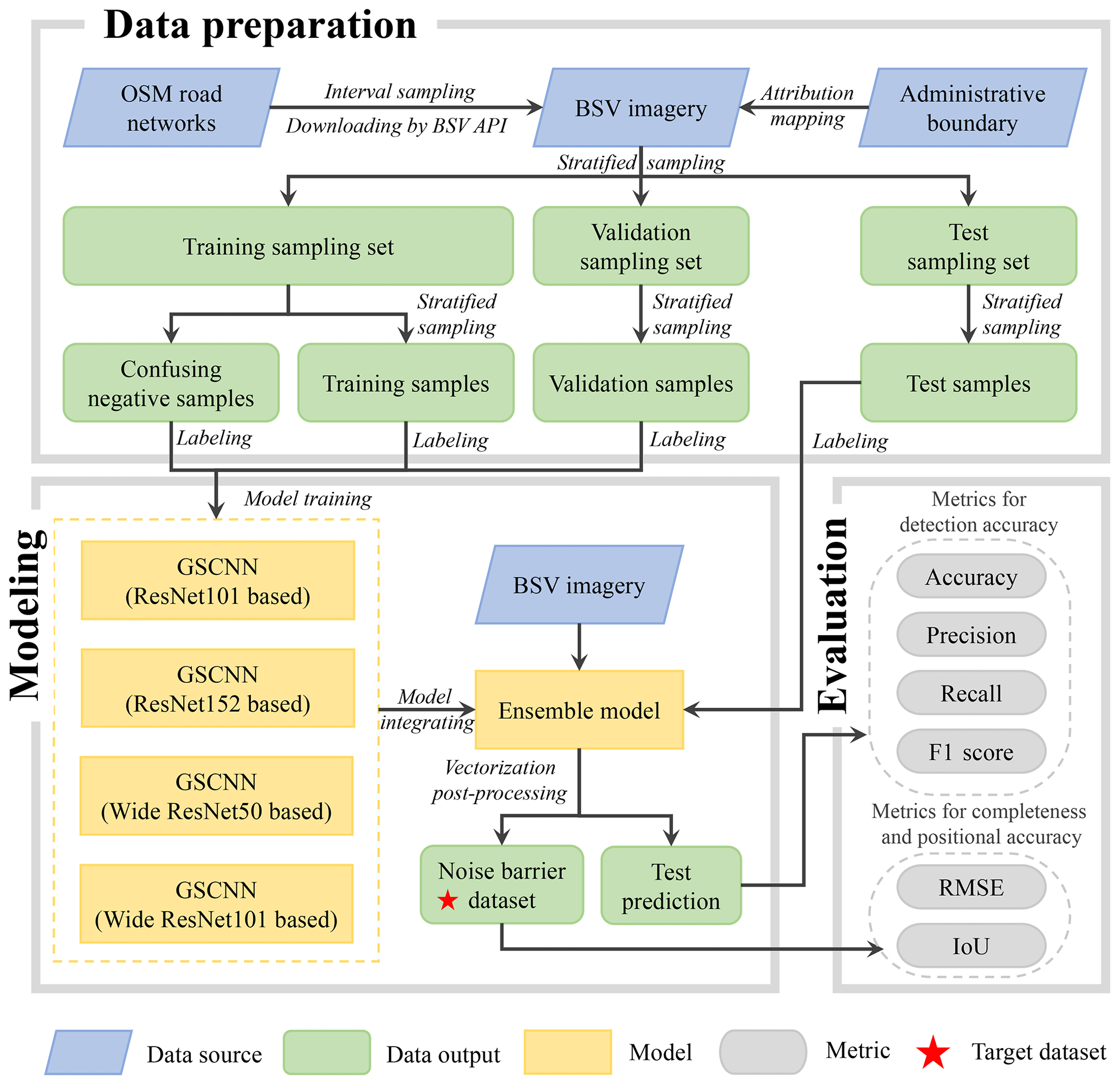
The GeoAI framework's workflow is divided into three stages: data preparation, modeling, and evaluation, as shown in Fig. 1. To begin with, BSV images are gathered during the data preparation stage using OpenStreetMap (OSM) road data and the BSV application programming interface (API). Subsequently, BSV images are used to generate various samples for modeling and evaluation. During the modeling stage, deep learning approaches are used to detect RNBs from the BSV imagery. Using the vectorization post-processing method, the identified and scattered RNB locations are subsequently processed into a vectorized dataset. During the evaluation stage, the quality of the created dataset is quantitatively assessed in two aspects, i.e., the detection accuracy and completeness and positional accuracy.
2.2 Data preparation
There are three types of data are acquired for this study, i.e., the road networks, administrative boundary, and street view imagery. Afterwards, training, validation, and test samples are collected based on these data. The data from Taiwan Province are scarce.
2.2.1 Road networks
The road networks were downloaded from OSM (https://www.openstreetmap.org/, last access: 16 May 2021) in May 2021, which are polyline-based and include a variety of road types, including motorways, trunk roads, primary roads, and secondary roads. According to previous findings, the quality of OSM road networks in China is high in terms of completeness and positional accuracy (Liu and Long, 2015). In addition, RNBs have a high probability of being installed on motorways and trunk roads (K. Zhang et al., 2022). Therefore, given the expense of acquiring and computing BSV images, in this study, samples on motorways and trunk roads are only considered for downloading BSV images. Figure 2a depicts the spatial distribution of these two types of roads.
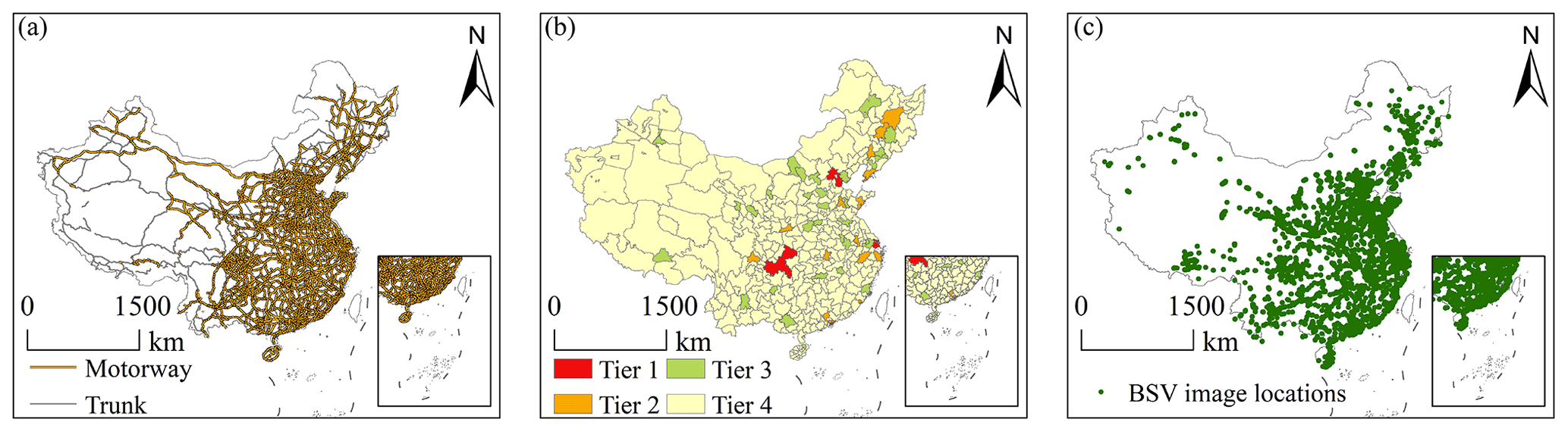
Figure 2There are three data sources used in this study. OSM road network data (a), the Chinese administrative boundary, with four city tiers (b), and the spatial distribution of the BSV image locations (c) are shown. Road networks are from © OpenStreetMap contributors (2022) and distributed under the Open Data Commons Open Database License (ODbL) v1.0.
2.2.2 Administrative boundary
The city boundary was acquired from http://bzdt.ch.mnr.gov.cn/ (last access: 21 April 2021) in April 2021. According to the urban management hierarchy established by the Chinese government, cities in China are divided into four tiers (Guan and Rowe, 2018; Jia et al., 2020), including municipalities, sub-provincial cities, and prefecture-level cities, and their locations are shown in Fig. 2b. Specifically, tier 1 is centrally administered cities and municipalities. Tier 2 is primarily sub-provincial cities, whereas tier 3 is province capitals and large prefecture-level cities. Tier 4 is ordinary prefecture cities. Cities with varying administrative levels have varying authorities over resource allocation and jurisdiction (Guan et al., 2018).
2.2.3 Street view imagery
With their high-resolution and detailed information on Chinese streets, BSV images are of comparable quality to Google Street View images, which are not available in China (H. Zhou et al., 2019). Numerous sample points along OSM roads are collected, and the BSV API is utilized to obtain street view images at those locations. Following the work of K. Zhang et al. (2022), a sampling interval of around 25 m is utilized to account for the tradeoff between data granularity and the expense of downloading imagery. As a result, the total number of sample points is 24 871 839. As shown in Fig. 3, an illustration of the BSV images, with photographs showing different directions, shows that a BSV image with a 90∘ viewing angle is more appropriate for the present work because it provides a comprehensive roadside view. Hence, to identify the RNBs along the corresponding roadside, BSV images with a 90∘ viewing angle are acquired. Owing to the absence of BSV images on a few road segments in a particular year, these will be supplemented in adjacent years. Additionally, the BSV sensors may be obstructed by some vehicles or other surrounding objects. These issues are resolved through the use of multitemporal BSV images (ones from 2013 to 2021 are downloaded in this study). A total of 6 008 674 BSV images are downloaded with a size of 500 pixels × 400 pixels, and their spatial locations are shown in Fig. 2c. Figure 4 depicts the spatial distribution of the number of BSV images in China, with the eastern region and higher city tiers having a greater number of BSV images.

Figure 3Illustration of BSV images, with photographs showing different directions (BSV images are from © Baidu Maps, 2022).
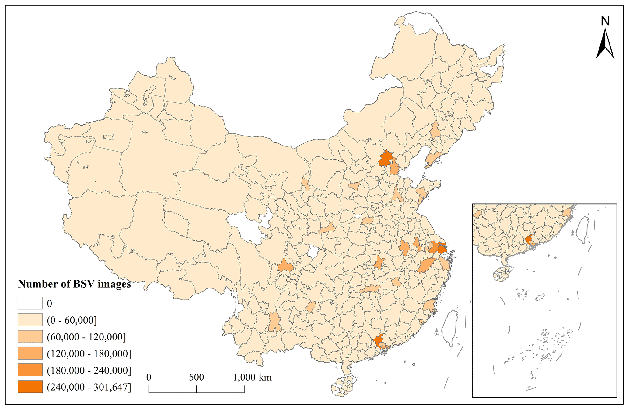
Figure 4Zonal statistics of the number of BSV images in China.
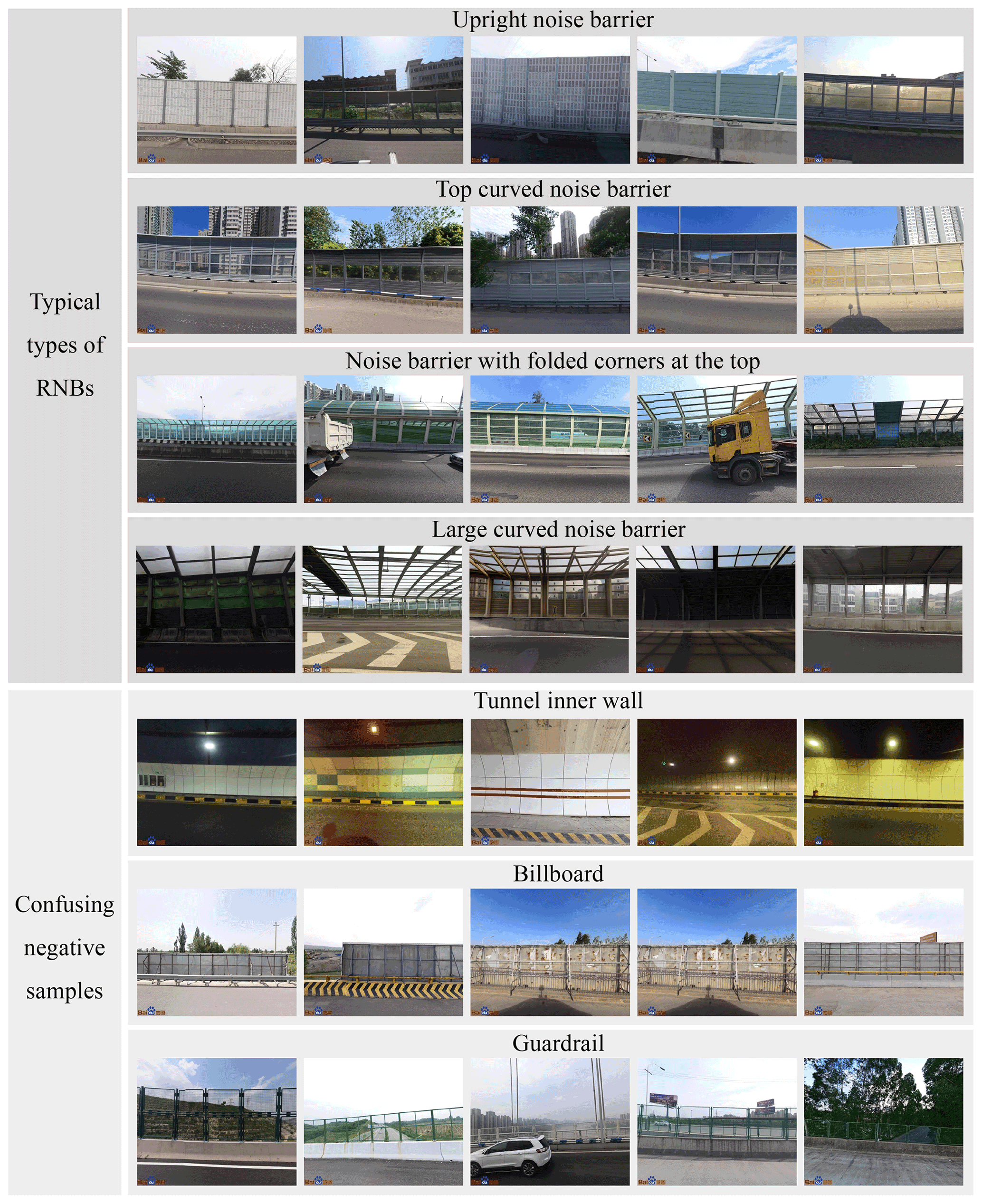
Figure 5Illustration of BSV samples, including four typical types of RNBs based on physical shapes (a) and three types of confusing negative samples which look like RNBs (b) (BSV images are from © Baidu Maps, 2022).
2.2.4 Training, validation, and test sample collection
An effective sampling technique for generating training, validation, and test image samples is developed to detect RNBs from the large volume of BSV images collected. According to their physical shapes, the RNBs identified in this study can be categorized into the following four distinct types: upright noise barrier, top curved noise barrier, noise barrier with folded corners at the top, and large curved noise barrier, as depicted in Fig. 5. Figure 1 illustrates the different steps followed in the data preparation stage. The BSV images are classified into four tiers based on their location within the city administration hierarchy. Subsequently, the training, validation, and test sampling set are subdivided from the entire images, accounting for 60 %, 20 %, and 20 % of images, respectively. These sampling sets can be used to collect the corresponding samples and are beneficial in that they avoid the mixing of samples.
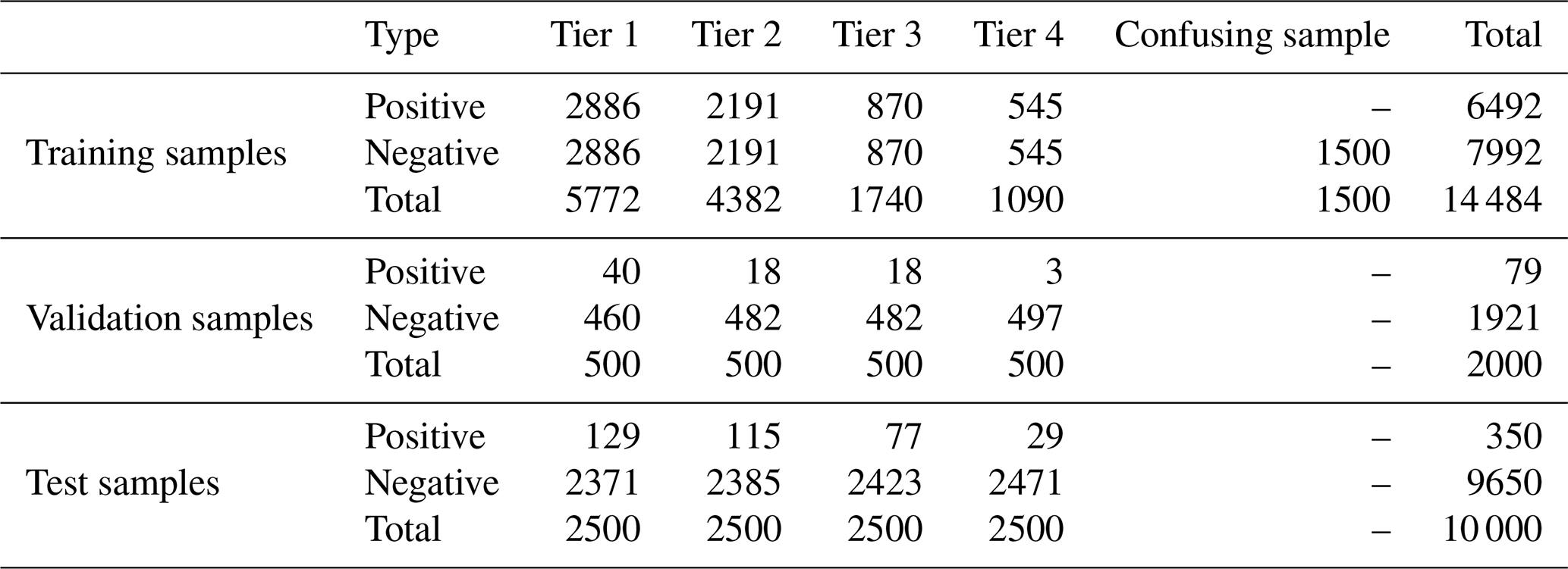
Previous investigations revealed that BSV images with RNBs are rare, accounting for less than 5 % of the sampled images. To alleviate the impact of the class imbalance problem on model training, 50 000 images are randomly selected from each city tier based on the training sampling set. These samples are labeled as positive type (i.e., image with RNB) or negative type (i.e., image without RNB) by manual visual interpretation, the details of which are shown in Fig. 6. Subsequently, the same number of positive and negative samples are maintained. Certain objects, such as tunnel inner walls, billboards, and guardrails, seem like RNBs in images, which intensifies the difficulty of deep learning, as shown in Fig. 5. Therefore, 500 images of each of these objects are added as confusing negative samples to the training samples. The ultimate training sample size is 14 484, including 6492 positive and 7992 negative samples. To generate the validation and test samples, 500 and 2500 image samples from each city tier are chosen. There are 79 positive samples and 1921 negative samples in the validation samples, while there are 350 positive samples and 9650 negative samples in the test samples. The details of the sample collection results are shown in Table 1. The labeled BSV images are available at https://doi.org/10.11888/Others.tpdc.271914 (Chen, 2021).


Figure 7The construction of the convolutional neural network incorporating image background information (BSV images are from © Baidu Maps, 2022).
2.3 Modeling
2.3.1 Convolutional neural network incorporating image context information (IC-CNN)
RNBs are widely placed on the roadside in densely populated regions, such as residential areas and educational and government institutions, as previously described in other studies (Arenas, 2008; Wang et al., 2018; K. Zhang et al., 2022). Therefore, based on this prior geographic knowledge, an IC-CNN that leverages the context information contained in BSV images is developed which aims at enhancing the RNB detection accuracy. Figure 7 illustrates the construction of IC-CNN, which adopts the ResNet architecture (He et al., 2016). In this workflow, prior geographic knowledge is incorporated into the neural network by means of transferring learning. Initially, 500 samples are randomly selected from positive and negative training samples in each tier. There are three context labels added, depending on the context of these BSV images, i.e., building dominated, non-building dominated, and uncertain (unable to judge the background of the BSV image because it is obscured by objects), as shown in Fig. 6. The context labels are interpreted by semantic segmentation models released by the MIT Computer Vision team (B. Zhou et al., 2019). Besides the sky and ground objects, images are judged to be building dominated if the ratio of building objects is the most; otherwise, they are evaluated to be non-building dominated. Additionally, the uncertain type is classified by a visual interpretation of whether the background environment in the image is obscured. These labeled images are available at https://doi.org/10.11888/Others.tpdc.271914 (Chen, 2021). Next, 4000 samples with image context labels are used to train the IC-CNN on a preliminary basis, using hybrid loss to optimize the parameters in IC-CNN for image context and RNB identification, as formulated in Eq. (1). After the network has converged, the IC-CNN's classifier is replaced with a binary classification, and all the training samples are supplemented to fine-tune and intensively train the network.
where pimage context is the confidence of the image context identification, pnoise barrier is the confidence of the RNB identification, and CE(p) refers to the cross-entropy loss function (Hu et al., 2018).
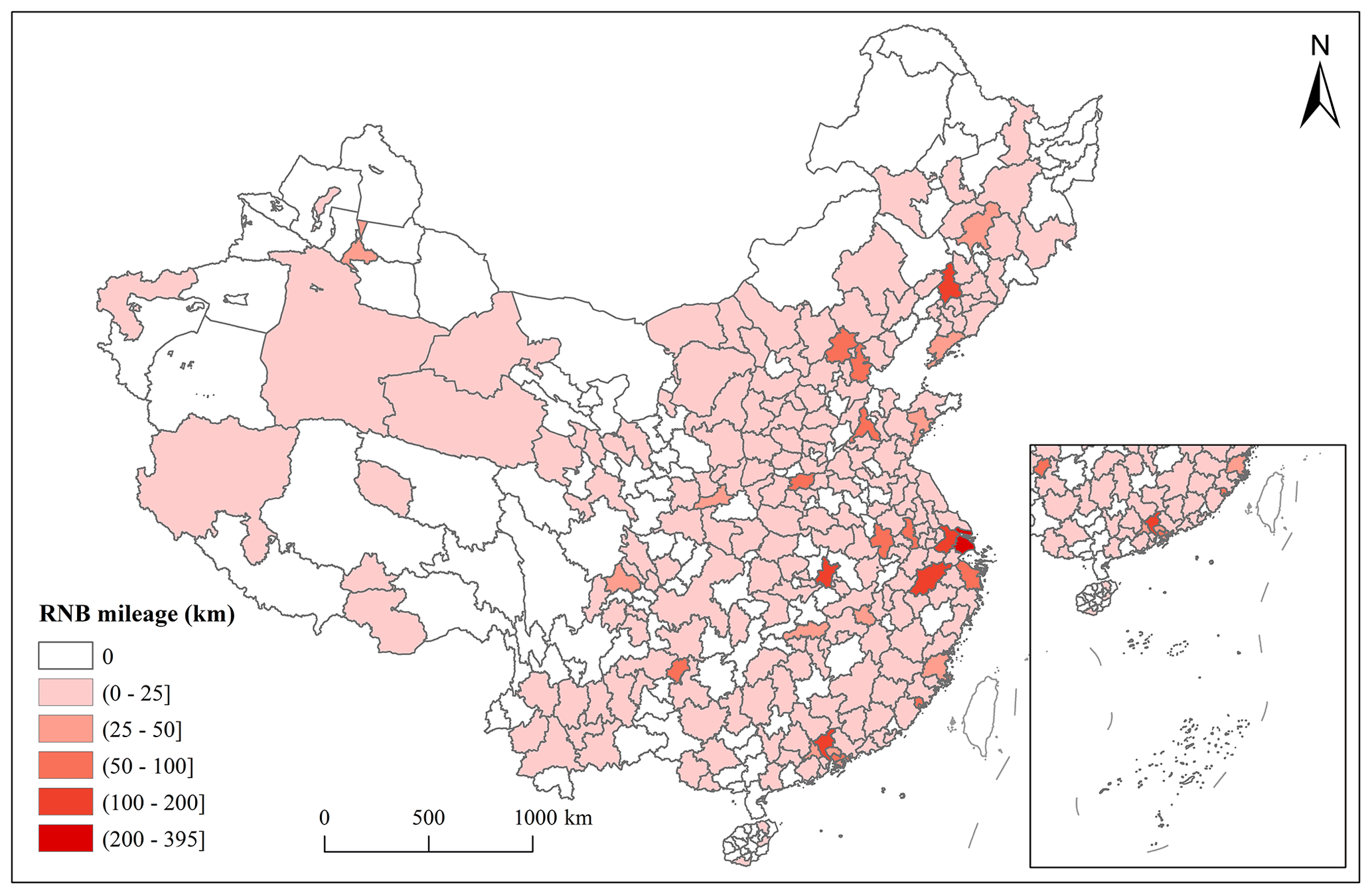
Figure 8Zonal statistics of RNB mileage in China. The blank areas indicate no RNBs or a lack of BSV images.
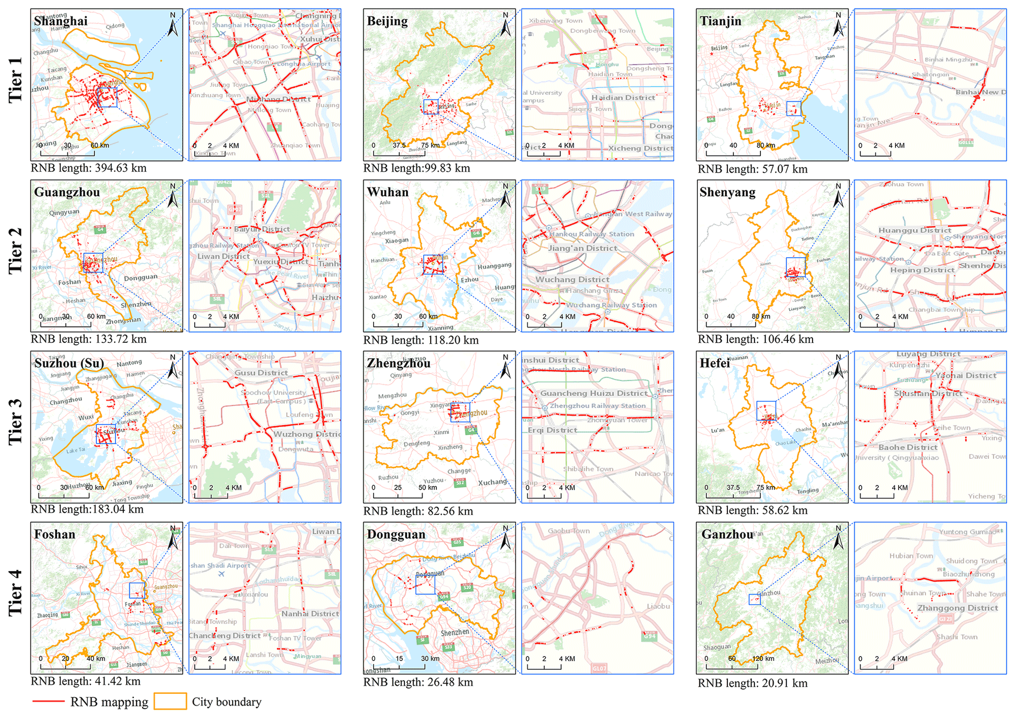
Figure 9Distribution of RNBs in several representative cities (base maps are from Esri).
2.3.2 Ensemble learning strategy
Owing to the high cost of labeling and the restricted quantity of trained samples, an ensemble learning strategy for enhancing RNB detection accuracy is utilized in this study based on the “no free lunch” theory (Wolpert and Macready, 1997). In an ensemble learning domain, the effective strategy to boost performance is to integrate the numerous high-variance models together (Cao et al., 2020). Therefore, this study integrates four IC-CNNs, and their convolutional layers are chosen from the ResNet family (He et al., 2016; Zagoruyko and Komodakis, 2016), including ResNet101, ResNet152, Wide ResNet50, and Wide ResNet101. The integration of the four IC-CNNs with varying capacities for feature extraction can make a significant contribution to achieving high detection accuracy.
2.3.3 Vectorization post-processing
After performing a detection run by an ensemble of IC-CNNs, the identified and scattered RNB locations are connected to create a vectorized RNB dataset by a post-processing technique, which is based on the spatial neighbor relationship between samples. Specifically, if adjacent sample images of the same road contain RNB objects, their locations will be connected. Furthermore, the findings of Sainju and Jiang (2020) demonstrated that the “near objects are more related” principle (Tobler, 1970, 2004) holds true when using street view imagery to detect objects at the urban scale. Therefore, in this study, given the likelihood of RNB misidentification, if a sample image is flanked by images containing RNBs in the same road, it will be considered as a positive type to minimize the impact of misidentification.
2.4 Evaluation methods
2.4.1 Metrics for detection accuracy
To evaluate the accuracy of RNB detection, four quantitative metrics in the deep learning classification task, including overall accuracy (OA), recall, precision, and F1 score (Thomas et al., 2020) are analyzed. Due to the class imbalance problem in BSV images, OA is susceptible to being affected by a large number of sample types in this study (i.e., negative type sample). In comparison, precision and recall can concentrate on positive type samples. The F1 score is the most comprehensive of these metrics because it considers both precision and recall. After detecting the RNBs in BSV images, the number of false negative (FN), true negative (TN), true positive (TP), and false positive (FP) images is calculated. True positive means that the prediction and ground truth of images are both positive. Conversely, false negative means the predictions are negative while the ground truths are positive. The four metrics are calculated based on the following (Thomas et al., 2020):
2.4.2 Metrics for completeness and positional accuracy
To quantitatively evaluate the completeness and positional accuracy of generated RNBs, two quantitative metrics, including the root mean squared error (RMSE) and the intersection over union (IoU) are adopted (Rezatofighi et al., 2019). To calculate these metrics, numerous roads are selected from various cities and are surveyed manually as ground truths based on BSV imagery. Based on the mileage deviation and overlap relationship between the generated and surveyed RNBs, RMSE and IoU are calculated following Eqs. (7) and (8), respectively:
where m is the number of selected roads, li is the surveyed RNB mileage of the ith road, and is the generated RNB mileage of the ith road.
where Lintersection is intersection mileage of the generated and surveyed RNB, and Lunion is union mileage of the generated and surveyed RNB.
2.5 Implementation configuration
Several techniques to enhance the performance of the model throughout the training and inference stages are employed in this study. Data augmentation techniques such as random resized cropping and random horizontal flipping are utilized to increase the data volume and decrease model bias error. The model parameters are optimized using the cosine annealing learning rate scheduler (Bhattacharyya et al., 2021) and AdamW optimizer (Loshchilov and Hutter, 2017). Long training and inference resized tuning (Touvron et al., 2019) are employed to improve the model's performance. Finally, an ensemble of models identifies RNBs based on the voting mechanism.
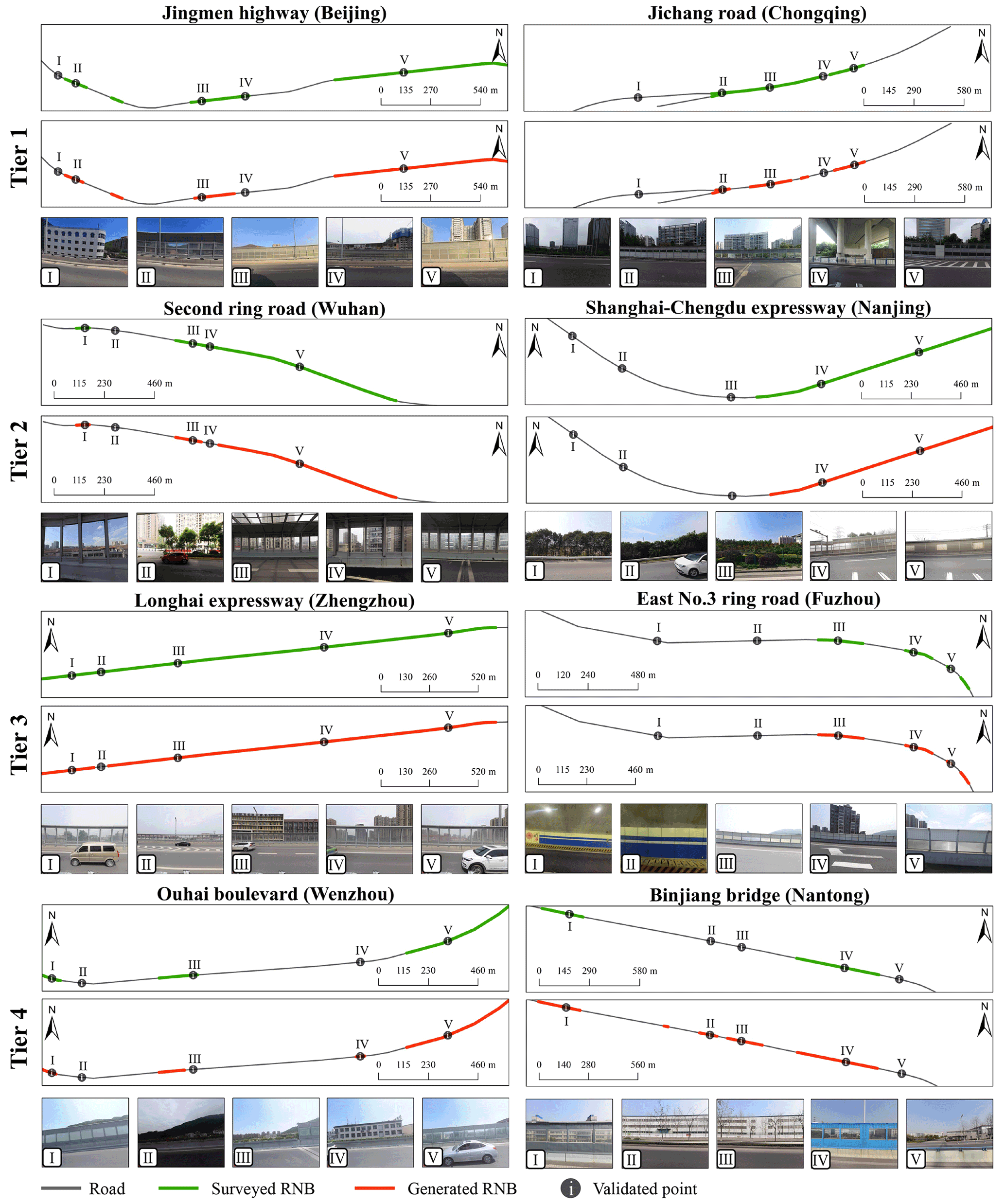
Figure 10RNB mapping result in the city scale (BSV images are from © Baidu Maps, 2022).
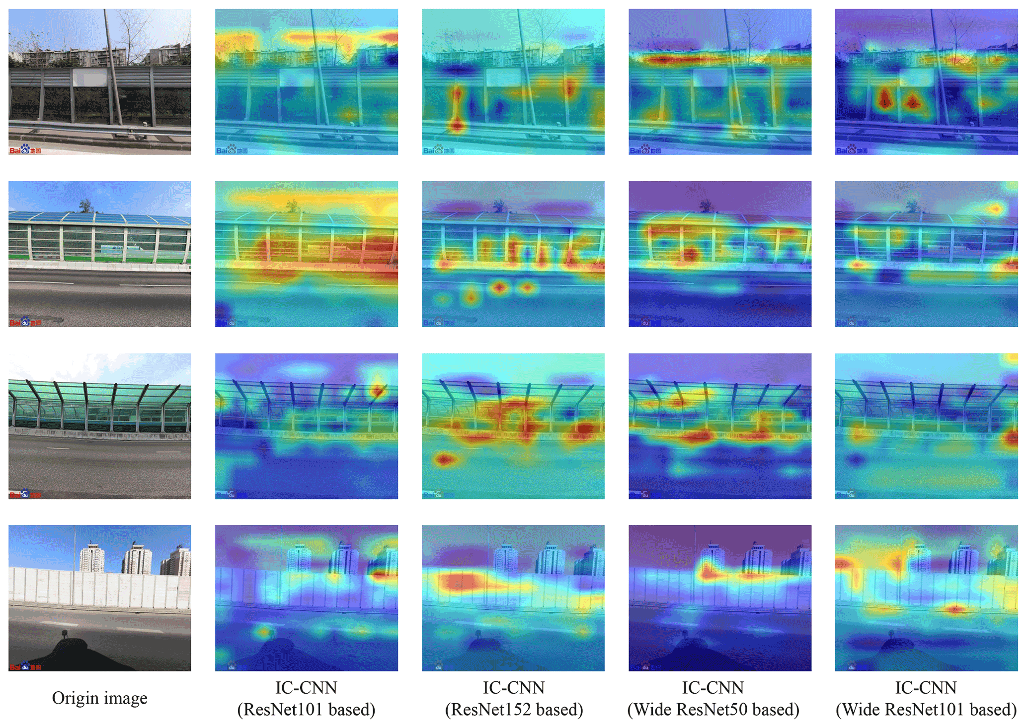
Figure 11Heat maps of IC-CNNs on BSV images with RNB. The hotspots indicate the area where the attention of IC-CNN is focused (BSV images are from © Baidu Maps, 2022).
3.1 RNB mapping result
The final RNBs dataset is available at https://doi.org/10.11888/Others.tpdc.271914 (Chen, 2021). Details of the BSV image identification results are shown in Appendix A, and details of RNB mileage by city in China are shown in Appendix B, with the total RNB mileage of 2667.02 km and the average RNB mileage for each city tier of 102.39 km (±117.83 km), 66.36 km (±18.70 km), 22.19 km (±12.52 km), and 1.12 km (±0.42 km), respectively. The quantitative results suggest that there are substantial variations between the different city tiers. Tiers 1 and 2 contain a major portion of the total RNB mileage compared with the other city tiers; moreover, confidence intervals show that the higher the city tier, the greater the difference in the level of RNB construction in that city tier. The reason for these variances is that the unique urban administration system in China mandates lower-tier cities to rigidly follow the leadership of higher-tier cities (Ma, 2005; Zhao et al., 2003). Higher-tier cities are rapidly increasing in size and occupying considerable resources, while lower-tier cities are developing slowly (Au and Henderson, 2006; Lin, 2002). The spatial distribution of RNB mileage among cities is further depicted in Fig. 8, where blank areas indicate the absence of RNBs or BSV images (there are 17 cities lacking BSV images, as shown in Appendix B). Figure 8 suggests that RNBs in eastern China are more densely distributed and have longer mileage. To a certain extent, it shows that the statistics correlate with the development of Chinese cities, implying that higher-tier cities have a high probability of covering and updating BSV imagery or laying down RNBs.
Table 2Evaluation results of RNB identification in different city tiers. The evaluation results of every city tier are calculated using the test samples of the corresponding city tier, while the overall evaluation results are calculated using the entire test samples.
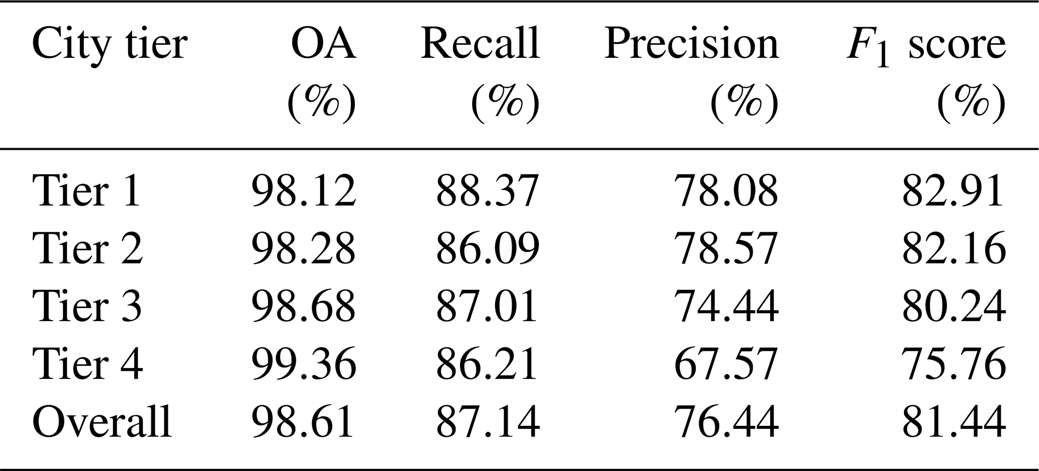
Table 3Ablation study design. The ablation study combines the four strategies used in this study to illustrate their effectiveness.
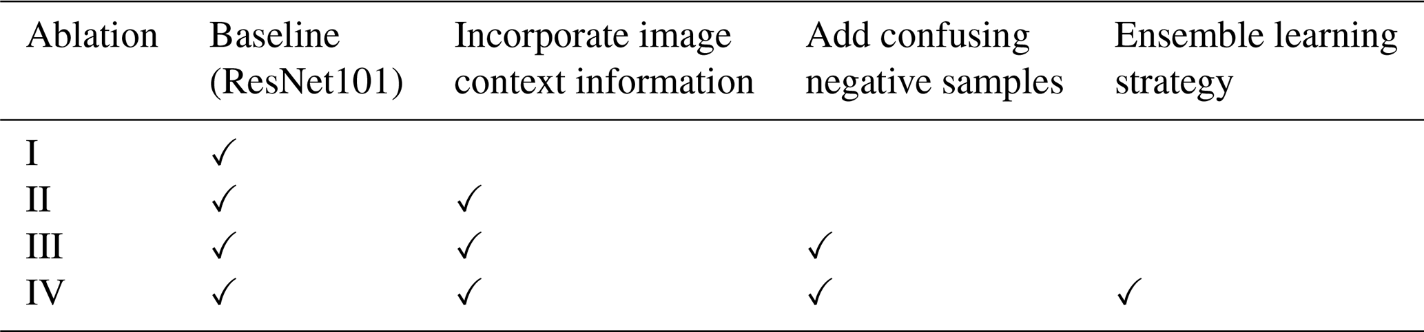
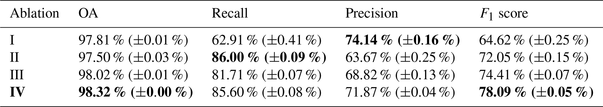
Table 4Quantitative results of ablation. The ablation results show that the proposed methods have the highest RNB detection accuracy. The bold values indicate the highest value in each metric.
After analyzing the generated RNB dataset from a national scale, three cities with the highest RNB mileage in each tier are selected to analyze the citywide mapping results, as shown in Fig. 9. The figure shows that RNBs are generally clustered in the central areas of these cities. For example, the RNBs in Shanghai are mainly clustered on the third ring road, while those in Beijing are mainly clustered on the sixth ring road. As a result, when combined with the planned layout and actual mapping of RNB distribution, the generated RNB dataset can partially reflect the rationality of urban infrastructure planning and layout.
3.2 Evaluation and analysis
3.2.1 RNB detection accuracy
Table 2 summarizes the evaluation results of the RNB identification at different city tiers based on test samples. The OA and the F1 score for the overall city tiers are 98.61 % and 81.44 %, respectively. However, the accuracy is greater for higher-tier cities than for lower-tier cities. This may be attributed to the fact that cities with lower tiers appear to have less RNB infrastructure, resulting in a more severe class imbalance problem for deep learning methods, which impacts the training and generalization of the model. Therefore, the results indicate that, prior to using this dataset, an assessment of the influence of regional quality differences on specific applications is required.
3.2.2 RNB completeness and positional accuracy
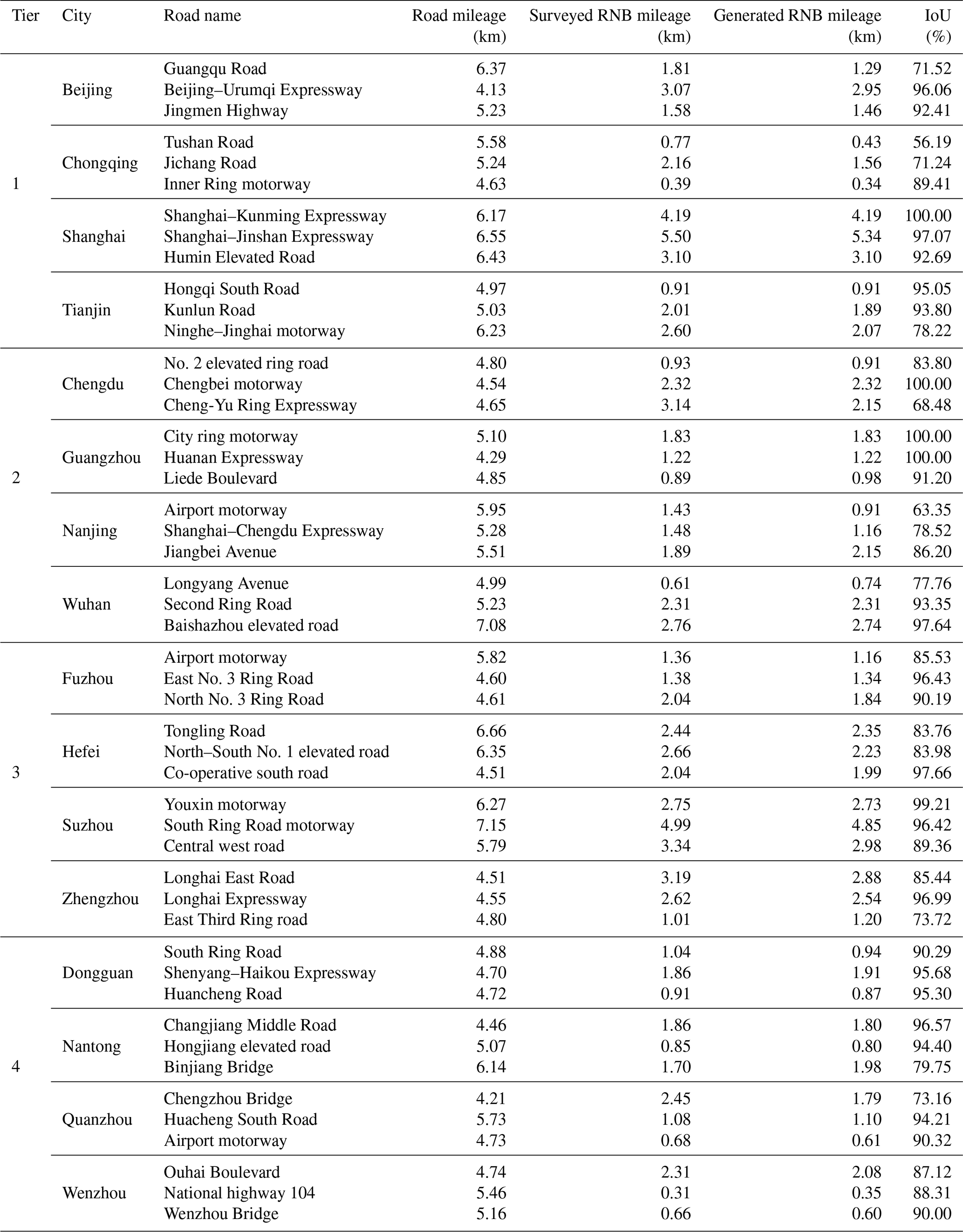
To evaluate the completeness and positional accuracy of the RNB dataset, approximately 254.45 km of roads are selected from different city tiers and manually surveyed using the BSV imagery. Appendix C summarizes the detailed quantitative differences between generated and surveyed RNBs in terms of mileage deviation and level of overlap. The overall RMSE for the mileage deviation is 0.08 km, and the IoU for the overlay level is 88.08 % ± 2.95 %. The results shows that the generated and surveyed RNBs are highly consistent in terms of mileage and distribution, demonstrating the high completeness and positional accuracy of the generated RNB dataset.
Moreover, as illustrated in Fig. 10, a visual comparison between surveyed and generated RNBs on various roads depicts that the generated and surveyed RNBs on the road are overall consistent in terms of mapping. However, several validated points demonstrated that the proposed deep learning approach incorrectly recognized small RNB objects in the images, such as validated points IV, II, and III on Beijing's Jingmen Highway, Zhengzhou's Longhai Expressway, and Wenzhou's Ouhai Boulevard, respectively. Additionally, several objects that looked similar to RNBs, such as multi-windowed buildings, are misclassified as a positive type, for example, point IV on Wenzhou's Ouhai Boulevard and points II and III on Nantong's Binjiang Bridge. Despite these misclassifications, most of the validated points demonstrated a high accuracy of the RNB prediction and the high performance of the proposed framework, implying the reliability of the generated RNB dataset.
4.1 Model capability
An ablation study is conducted to demonstrate the quality of the generated dataset and validate the effectiveness of developed methods (Table 3). As shown in Table 4, the combination of proposed strategies achieves the highest performance. The ablation results illustrate that the effectiveness of proposed strategies, including integrating image context information into CNN, adding confusing negative samples, and using an ensemble learning strategy. Additionally, Fig. 11 depicts the areas of the IC-CNN's attention, revealing that IC-CNNs not only have a capacity for focusing on RNB objects in BSV images but also have a sense of their surroundings. The results suggest the reliability of the generated dataset and partially decipher the “black box” of deep learning to explain the high performance of the developed methods. Notably, this study successfully achieves incorporating some of the prior geographic knowledge into the deep learning method. RNB detection accuracy can be increased further by combining more comprehensive knowledge of geographic scenes from BSV images into deep learning network, such as various geographic elements and processes and the associated construction theory (Lü et al., 2018).
Table 5Confidence assessment in the mapping accuracy for cities with low-mileage RNBs.

4.2 Limitations and future work
This study has several limitations in the process of dataset generation which can be grouped into three categories, namely data source, ground scenario, and modeling.
Due to the economic status, topographical conditions, or government policies, not all Chinese cities are covered by BSV imagery, with data not being available for 17 cities (Deng et al., 2021; Du et al., 2020). In addition, challenges owing to overexposure or obstruction of the sensors by vehicles hinder the capturing of a complete street scene. As a result, the natural characteristics of the data source can have certain impacts on the accuracy of the RNB dataset.
The road/traffic environment is often complex. Concretely, BSV sensors can detect RNBs on distant highways or other lanes, and it may result in some mistakes during RNB detection and mapping. However, the likelihood of this occurring is small (about 4 % of RNB samples) by sampling investigation.
This study implicitly presupposes that BSV images are independent and identically distributed. As shown in Fig. 9, the developed GeoAI framework can achieve a high performance in continuous RNB mapping. However, the spatial autocorrelation effect in BSV images is overlooked, as BSV images taken along the same road network path frequently resemble the adjacent one (Sainju and Jiang, 2020).
Moreover, there are some uncertainties in cities with short mileage RNBs which may be generated due to misidentification. A manual survey is performed to verify the confidence level of these cities. Table 5 shows the quantitative results, which indicate that the shorter the RNBs, the lower the confidence level. In addition, the results show that the confidence level is lowest for cities with RNBs of less than 0.2 km, so further validation is needed when applying them in specific applications.
In the future, to address the data shortage issue, more data sources, such as Google Maps and Tencent Maps, will be used. Additionally, approaches for photogrammetry and image scene understanding techniques will be developed to tackle the complex ground scenario. Finally, end-to-end deep learning algorithms will be constantly enhanced by the addition of more powerful units and structures to account for spatial autocorrelation in street view imagery.
The road networks come from OSM (https://www.openstreetmap.org/, OpenStreetMap contributors, 2021), a collaborative project dedicated to providing many types of freely editable geographic data for the world. City boundaries can be obtained from http://bzdt.ch.mnr.gov.cn/ (Map Technical Review Center, Ministry of Natural Resources, China, 2021). In addition, BSV images can be downloaded by using BSV API (https://api.map.baidu.com/panorama/v2?key=parameters, Baidu Maps, 2022). Finally, the generated RNB dataset, labeled BSV image benchmark, and RNB detection results are available to the public at https://doi.org/10.11888/Others.tpdc.271914 (Chen, 2021). Specifically, the generated RNB dataset is grouped by city level, with attributes of city tier, city name, province, and RNB mileage; the image labels are documented in a *.csv file for a benchmark of the image context, and all images are categorized into specific folders. The RNB detection results include meta information of all BSV samples, such as longitude, latitude, city name, city tier, timing of imaging, and detection label (0 presents non-RNB type, while 1 presents RNB type). The mileage in RNB dataset is calculated with the Albers equal-area conical projection.
The codes of deep learning approaches in this study are available at https://doi.org/10.11888/Others.tpdc.271914 (Chen, 2021) and https://github.com/ChanceQZ/NoiseBarrierIdentification (last access: 20 January 2022). Python 3 packages such as PyTorch, NumPy, and OpenCV are used to develop the code. The vectorization post-processing procedure is performed in the ArcGIS Pro platform.
This study presents the first nationwide vectorized dataset of RNB and the benchmark dataset of the labeled BSV images in China using BSV imagery and a GeoAI framework. In this study, based on prior geographic knowledge in BSV imagery, RNB samples are identified based on deep learning approaches, and the vectorized RNB dataset is subsequently constructed using the vectorization post-processing procedure. The created RNB dataset is evaluated from two perspectives, i.e., the detection accuracy and the completeness and positional accuracy. The four quantitative metrics, OA, recall, precision, and F1 score, with values of 98.61 %, 87.14 %, 76.44 %, and 81.44 %, illustrate high accuracy of the model in RNB detection. The level of mileage deviation and overlay between the generated and surveyed RNBs are further determined via a manual survey of around 254.45 km of roads in various cities, with the RMSE of 0.08 km and IoU of 88.08 % ± 2.95 % revealing that the created and surveyed RNBs are consistent and reliable.
The intended applications for the two datasets are diverse. In terms of the vectorized dataset of RNBs, urban studies can benefit from accurate information of RNB mileage, location, and distribution. For example, the regional energy potential of solar photovoltaic panels on RNB can be estimated, finer 3D urban models are able to be developed, and the sustainability of urban layouts can be evaluated. On the other hand, the benchmark dataset of labeled BSV images may contribute to multiple other research and applications related to RNBs identification, such as developing advanced deep learning algorithms and fine-tuning existing computer vision models to detect RNBs more accurately and exploring the further relationship between the RNB locations and surrounding environment.

Table A2Identification of a confusion matrix based on test samples.

The total RNB mileage in China is 2667.02 km. The RNB mileage values in different city tiers are 614.34, 995.45, 710.25, and 346.32 km, respectively. The average RNB mileage values in different city tiers are 102.39 km (±117.83 km), 66.36 km (±18.70 km), 22.19 km (±12.52 km), and 1.12 km (±0.42 km), respectively.
Table B1Details of RNB mileage by city in China. The RNB mileage values of some cities are 0 km, indicating that they lack RNBs or BSV images or that the BSV images are out of date. Specifically, there are 17 cities lacking BSV images, e.g., Baisha, Baoting, Changjiang, Dingan, Ledong, Língāo, Sansha, Wenchang, Jiyuan, Daxing'anling, Shuangyashan, Guoluo, Huangnan, Bazhong, Nujiang, Zhoushan, Xinji.
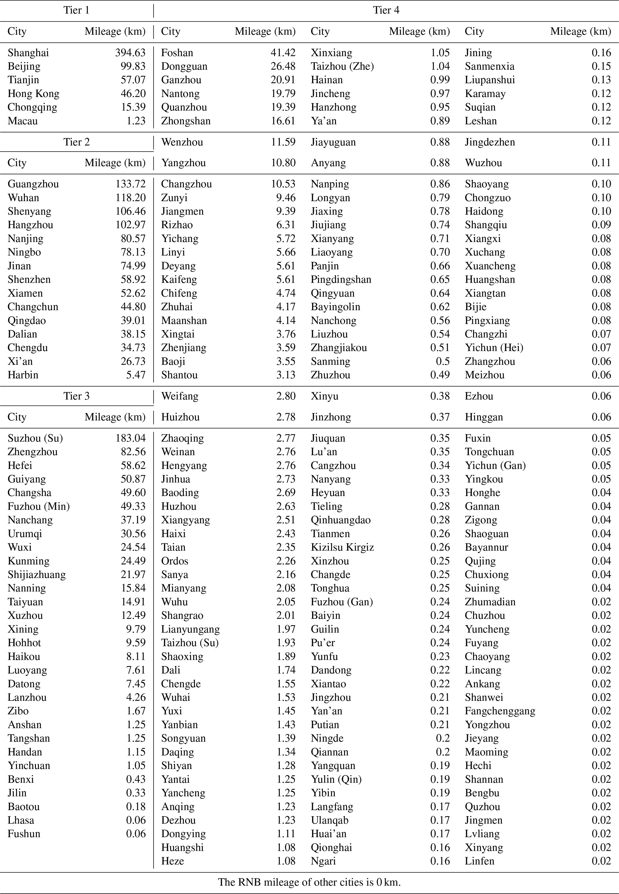
Table C1Quantitative comparison with the generated and surveyed RNBs in different roads in different city tiers. The 4–7.5 km of roads with RNBs are selected as surveyed objects. The total road mileage is around 254.45 km.
ZQ developed the framework, performed experiments, and wrote the original draft. MC conceptualized and supervised the project and contributed with the design of the work and the critical revision of the article, together with TZ, FZ, ZZ, and RZ. YYa and KZ collected and processed data source and published the dataset. ZS aided with the data preparation. PM aided in data collection and visualization. GL and YYe contributed with the technical review.
The contact author has declared that none of the authors has any competing interests.
Publisher’s note: Copernicus Publications remains neutral with regard to jurisdictional claims in published maps and institutional affiliations.
We appreciate the detailed suggestions and comments from the anonymous reviewers. We express heartfelt thanks to the other members of the Smart City Sensing and Simulation lab and OpenGMS lab, who undertook the data collection and annotation work. The data of this work are licensed and hosted by the National Tibetan Plateau Data Center.
This research has been supported by the National Natural Science Foundation of China and National Natural Science Foundation of China-Guangdong Joint Fund (grant no. U1811464) and the Postgraduate Research and Practice Innovation Program of Jiangsu Province (grant no. KYCX22_1567).
This paper was edited by Alexander Gruber and reviewed by two anonymous referees.
Abdulkareem, M., Havukainen, J., Nuortila-Jokinen, J., and Horttanainen, M.: Life cycle assessment of a low-height noise barrier for railway traffic noise, J. Clean. Prod., 323, 129169, https://doi.org/10.1016/j.jclepro.2021.129169, 2021.
Apparicio, P., Carrier, M., Gelb, J., Séguin, A.-M., and Kingham, S.: Cyclists' exposure to air pollution and road traffic noise in central city neighbourhoods of Montreal, J. Transp. Geogr., 57, 63–69, https://doi.org/10.1016/j.jtrangeo.2016.09.014, 2016.
Arenas, J. P.: Potential problems with environmental sound barriers when used in mitigating surface transportation noise, Sci. Total Environ., 405, 173–179, https://doi.org/10.1016/j.scitotenv.2008.06.049, 2008.
Au, C.-C. and Henderson, J. V.: Are Chinese cities too small?, Rev. Econ. Stud., 73, 549–576, https://doi.org/10.1111/j.1467-937X.2006.00387.x, 2006.
Baidu Maps: Baidu Street View, https://api.map.baidu.com/panorama/v2?key=parameters, last access: 13 June 2022.
Begou, P., Kassomenos, P., and Kelessis, A.: Effects of road traffic noise on the prevalence of cardiovascular diseases: The case of Thessaloniki, Greece, Sci. Total Environ., 703, 134477, https://doi.org/10.1016/j.scitotenv.2019.134477, 2020.
Bhattacharyya, A., Chatterjee, S., Sen, S., Sinitca, A., Kaplun, D., and Sarkar, R.: A deep learning model for classifying human facial expressions from infrared thermal images, Scientific Reports, 11, 20696, https://doi.org/10.1038/s41598-021-99998-z, 2021.
Den Boer, L. and Schroten, A.: Traffic noise reduction in Europe, CE Delft, 14, 2057–2068, https://inquinamentoacustico.it/_dowload/traffic_noise_reduction-CE-Delft.pdf (last access: 12 December 2021), 2007.
Cao, Y., Geddes, T. A., Yang, J. Y. H., and Yang, P.: Ensemble deep learning in bioinformatics, Nature Machine Intelligence, 2, 500–508, https://doi.org/10.1038/s42256-020-0217-y, 2020.
Chen, M.: Vectorized dataset of roadside noise barriers in China, National Tibetan Plateau/Third Pole Environment Data Center [data set], https://doi.org/10.11888/Others.tpdc.271914, 2021.
Deng, M., Yang, W., Chen, C., Wu, Z., Liu, Y., and Xiang, C.: Street-level solar radiation mapping and patterns profiling using Baidu Street View images, Sustain. Cities Soc., 75, 103289, https://doi.org/10.1016/j.scs.2021.103289, 2021.
Du, K., Ning, J., and Yan, L.: How long is the sun duration in a street canyon? – Analysis of the view factors of street canyons, Build. Environ., 172, 106680, https://doi.org/10.1016/j.buildenv.2020.106680, 2020.
Goodchild, M. F. and Li, W.: Replication across space and time must be weak in the social and environmental sciences, P. Natl. Acad. of Sci. USA, 118, e2015759118, https://doi.org/10.1073/pnas.2015759118, 2021.
Griffiths, D. and Boehm, J.: Improving public data for building segmentation from Convolutional Neural Networks (CNNs) for fused airborne lidar and image data using active contours, ISPRS J. Photogramm., 154, 70–83, https://doi.org/10.1016/j.isprsjprs.2019.05.013, 2019.
Gu, M., Liu, Y., Yang, J., Peng, L., Zhao, C., Yang, Z., Yang, J., Fang, W., Fang, J., and Zhao, Z.: Estimation of environmental effect of PVNB installed along a metro line in China, Renew. Energ., 45, 237–244, https://doi.org/10.1016/j.renene.2012.02.021, 2012.
Guan, C. and Rowe, P. G.: In pursuit of a well-balanced network of cities and towns: A case study of the Changjiang Delta Region in China, Environ. Plann. B, 45, 548–566, https://doi.org/10.1177/2399808317696073, 2018.
Guan, X., Wei, H., Lu, S., Dai, Q., and Su, H.: Assessment on the urbanization strategy in China: Achievements, challenges and reflections, Habitat Int., 71, 97–109, https://doi.org/10.1016/j.habitatint.2017.11.009, 2018.
He, K., Zhang, X., Ren, S., and Sun, J.: Deep Residual Learning for Image Recognition, 2016 IEEE Conference on Computer Vision and Pattern Recognition (CVPR), Las Vegas, NV, USA, 27–30 June 2016, 770–778, https://doi.org/10.1109/CVPR.2016.90, 2016.
Hu, K., Zhang, Z., Niu, X., Zhang, Y., Cao, C., Xiao, F., and Gao, X.: Retinal vessel segmentation of color fundus images using multiscale convolutional neural network with an improved cross-entropy loss function, Neurocomputing, 309, 179–191, https://doi.org/10.1016/j.neucom.2018.05.011, 2018.
Huang, Y., Lei, C., Liu, C. H., Perez, P., Forehead, H., Kong, S., and Zhou, J. L.: A review of strategies for mitigating roadside air pollution in urban street canyons, Environ. Pollut., 280, 116971, https://doi.org/10.1016/j.envpol.2021.116971, 2021.
Janowicz, K., Gao, S., McKenzie, G., Hu, Y., and Bhaduri, B.: GeoAI: spatially explicit artificial intelligence techniques for geographic knowledge discovery and beyond, Int. J. Geogr. Inf. Sci., 34, 625–636, https://doi.org/10.1080/13658816.2019.1684500, 2019.
Jia, M., Liu, Y., Lieske, S. N., and Chen, T.: Public policy change and its impact on urban expansion: An evaluation of 265 cities in China, Land Use Policy, 97, 104754, https://doi.org/10.1016/j.landusepol.2020.104754, 2020.
Kang, Y., Zhang, F., Gao, S., Lin, H., and Liu, Y.: A review of urban physical environment sensing using street view imagery in public health studies, Annals of GIS, 26, 261–275, https://doi.org/10.1080/19475683.2020.1791954, 2020.
Lafia, S., Turner, A., and Kuhn, W.: Improving Discovery of Open Civic Data, in: 10th International Conference on Geographic Information Science (GIScience 2018), Schloss Dagstuhl–Leibniz-Zentrum fuer Informatik, UC Santa Barbara, https://doi.org/10.4230/LIPIcs.GISCIENCE.2018.9, 2018.
LeCun, Y., Bengio, Y., and Hinton, G.: Deep learning, Nature, 521, 436–444, https://doi.org/10.1038/nature14539, 2015.
Li, W.: GeoAI: Where machine learning and big data converge in GIScience, Journal of Spatial Information Science, 20, 71–77, https://doi.org/10.5311/josis.2020.20.658, 2020.
Lin, G. C.: The growth and structural change of Chinese cities: a contextual and geographic analysis, Cities, 19, 299–316, https://doi.org/10.1016/S0264-2751(02)00039-2, 2002.
Liu, X. and Long, Y.: Automated identification and characterization of parcels with OpenStreetMap and points of interest, Environ. Plann. B, 43, 341–360, https://doi.org/10.1177/0265813515604767, 2015.
Liu, X., Chen, M., Claramunt, C., Batty, M., Kwan, M.-P., Senousi, A. M., Cheng, T., Strobl, J., Arzu, C., and Wilson, J.: Geographic information science in the era of geospatial big data: A cyberspace perspective, The Innovation, 3, 100279, https://doi.org/10.1016/j.xinn.2022.100279, 2022.
Liu, Y., Ma, X., Shu, L., Yang, Q., Zhang, Y., Huo, Z., and Zhou, Z.: Internet of things for noise mapping in smart cities: state of the art and future directions, IEEE Network, 34, 112–118, https://doi.org/10.1109/MNET.011.1900634, 2020.
Loshchilov, I. and Hutter, F.: Decoupled weight decay regularization, arXiv [preprint], https://doi.org/10.48550/arXiv.1711.05101, 14 November 2017.
Lü, G., Chen, M., Yuan, L., Zhou, L., Wen, Y., Wu, M., Hu, B., Yu, Z., Yue, S., and Sheng, Y.: Geographic scenario: a possible foundation for further development of virtual geographic environments, Int. J. Digit. Earth, 11, 356–368, https://doi.org/10.1080/17538947.2017.1374477, 2018.
Ma, L. J.: Urban administrative restructuring, changing scale relations and local economic development in China, Polit. Geogr., 24, 477–497, https://doi.org/10.1016/j.polgeo.2004.10.005, 2005.
Map Technical Review Center, Ministry of Natural Resources, China: Chinese administrative boundary, http://bzdt.ch.mnr.gov.cn/, last access: 21 April 2021.
Ning, Z., Hudda, N., Daher, N., Kam, W., Herner, J., Kozawa, K., Mara, S., and Sioutas, C.: Impact of roadside noise barriers on particle size distributions and pollutants concentrations near freeways, Atmos. Environ., 44, 3118–3127, https://doi.org/10.1016/j.atmosenv.2010.05.033, 2010.
Oltean-Dumbrava, C. and Miah, A.: Assessment and relative sustainability of common types of roadside noise barriers, J. Clean. Prod., 135, 919–931, https://doi.org/10.1016/j.jclepro.2016.06.107, 2016.
OpenStreetMap contributors: Data networks, OSM [data set], https://www.openstreetmap.org/, last access: 16 May 2021.
Perkins, R. M. and Xiang, W.-N.: Building a geographic info-structure for sustainable development planning on a small island developing state, Landscape Urban Plan., 78, 353–361, https://doi.org/10.1016/j.landurbplan.2005.10.005, 2006.
Potvin, S., Apparicio, P., and Séguin, A.-M.: The spatial distribution of noise barriers in Montreal: A barrier to achieve environmental equity, Transportation Res. D-T. E., 72, 83–97, https://doi.org/10.1016/j.trd.2019.04.011, 2019.
Qian, Z., Liu, X., Tao, F., and Zhou, T.: Identification of Urban Functional Areas by Coupling Satellite Images and Taxi GPS Trajectories, Remote Sensing, 12, 2449, https://doi.org/10.3390/rs12152449, 2020.
Qian, Z., Chen, M., Zhong, T., Zhang, F., Zhu, R., Zhang, Z., Zhang, K., Sun, Z., and Lü, G.: Deep Roof Refiner: A detail-oriented deep learning network for refined delineation of roof structure lines using satellite imagery, Int. J. Appl. Earth Obs., 107, 102680, https://doi.org/10.1016/j.jag.2022.102680, 2022
Qin, K., Xu, Y., Kang, C., and Kwan, M. P.: A graph convolutional network model for evaluating potential congestion spots based on local urban built environments, Transactions in GIS, 24, 1382–1401, https://doi.org/10.1111/tgis.12641, 2020.
Ranasinghe, D., Lee, E. S., Zhu, Y., Frausto-Vicencio, I., Choi, W., Sun, W., Mara, S., Seibt, U., and Paulson, S. E.: Effectiveness of vegetation and sound wall-vegetation combination barriers on pollution dispersion from freeways under early morning conditions, Sci. Total Environ., 658, 1549–1558, https://doi.org/10.1016/j.scitotenv.2018.12.159, 2019.
Rezatofighi, H., Tsoi, N., Gwak, J., Sadeghian, A., Reid, I., and Savarese, S.: Generalized intersection over union: A metric and a loss for bounding box regression, in: Proceedings of the IEEE/CVF Conference on Computer Vision and Pattern Recognition, Long Beach, CA, USA 15–20 June 2019, https://doi.org/10.1109/CVPR.2019.00075, 658–666, 2019.
Sainju, A. M. and Jiang, Z.: Mapping Road Safety Features from Streetview Imagery: A Deep Learning Approach, ACM/IMS Trans. Data Sci., 1, 15, https://doi.org/10.1145/3362069, 2020.
Song, Y. and Wu, P.: Earth Observation for Sustainable Infrastructure: A Review, Remote Sensing, 13, 1528, https://doi.org/10.3390/rs13081528, 2021.
Song, Y., Thatcher, D., Li, Q., McHugh, T., and Wu, P.: Developing sustainable road infrastructure performance indicators using a model-driven fuzzy spatial multi-criteria decision making method, Renew. Sust. Energ. Rev., 138, 110538, https://doi.org/10.1016/j.rser.2020.110538, 2021.
Thomas, K. A., Kidziński, Ł., Halilaj, E., Fleming, S. L., Venkataraman, G. R., Oei, E. H., Gold, G. E., and Delp, S. L.: Automated classification of radiographic knee osteoarthritis severity using deep neural networks, Radiology: Artificial Intelligence, 2, e190065, https://doi.org/10.1148/ryai.2020190065, 2020.
Tobler, W.: A computer movie simulating urban growth in the Detroit region, Econ. Geogr., 46, 234–240, 1970.
Tobler, W.: On the first law of geography: A reply, Ann. Assoc. Am. Geogr., 94, 304–310, https://doi.org/10.1111/j.1467-8306.2004.09402009.x, 2004.
Touvron, H., Vedaldi, A., Douze, M., and Jégou, H.: Fixing the train-test resolution discrepancy, arXiv [preprint], https://doi.org/10.48550/arXiv.1906.06423, 14 June 2019.
Wang, M., Deng, Y., Won, J., and Cheng, J. C.: An integrated underground utility management and decision support based on BIM and GIS, Automat. Constr., 107, 102931, https://doi.org/10.1016/j.autcon.2019.102931, 2019.
Wang, S. and Wang, X.: Modeling and analysis of highway emission dispersion due to noise barrier and automobile wake effects, Atmos. Pollut. Res., 12, 67–75, https://doi.org/10.1016/j.apr.2020.08.013, 2021.
Wang, Y., Zhu, X., Zhang, T., Bano, S., Pan, H., Qi, L., Zhang, Z., and Yuan, Y.: A renewable low-frequency acoustic energy harvesting noise barrier for high-speed railways using a Helmholtz resonator and a PVDF film, Appl. Energ., 230, 52–61, https://doi.org/10.1016/j.apenergy.2018.08.080, 2018.
Wang, Y.-R. and Li, X.-M.: Arctic sea ice cover data from spaceborne synthetic aperture radar by deep learning, Earth Syst. Sci. Data, 13, 2723–2742, https://doi.org/10.5194/essd-13-2723-2021, 2021.
Wolpert, D. H. and Macready, W. G.: No free lunch theorems for optimization, IEEE T. Evolut. Comput., 1, 67–82, https://doi.org/10.1109/4235.585893, 1997.
Zagoruyko, S. and Komodakis, N.: Wide residual networks, arXiv [preprint], https://doi.org/10.48550/arXiv.1605.07146, 23 May 2016.
Zhang, F., Zhou, B., Liu, L., Liu, Y., Fung, H. H., Lin, H., and Ratti, C.: Measuring human perceptions of a large-scale urban region using machine learning, Landscape Urban Plan., 180, 148–160, https://doi.org/10.1016/j.landurbplan.2018.08.020, 2018.
Zhang, F., Wu, L., Zhu, D., and Liu, Y.: Social sensing from street-level imagery: A case study in learning spatio-temporal urban mobility patterns, ISPRS J. Photogramm., 153, 48–58, https://doi.org/10.1016/j.isprsjprs.2019.04.017, 2019.
Zhang, K., Qian, Z., Yang, Y., Chen, M., Zhong, T., Zhu, R., Lv, G., and Yan, J.: Using street view images to identify road noise barriers with ensemble classification model and geospatial analysis, Sustain. Cities Soc., 78, 103598, https://doi.org/10.1016/j.scs.2021.103598, 2022.
Zhang, Z., Qian, Z., Zhong, T., Chen, M., Zhang, K., Yang, Y., Zhu, R., Zhang, F., Zhang, H., Zhou, F., Yu, J., Zhang, B., Lü, G., and Yan, J.: Vectorized rooftop area data for 90 cities in China, Scientific Data, 9, 66, https://doi.org/10.1038/s41597-022-01168-x, 2022.
Zhao, S. X., Chan, R. C., and Sit, K. T.: Globalization and the dominance of large cities in contemporary China, Cities, 20, 265–278, https://doi.org/10.1016/S0264-2751(03)00031-3, 2003.
Zhao, W.-J., Liu, E.-X., Poh, H. J., Wang, B., Gao, S.-P., Png, C. E., Li, K. W., and Chong, S. H.: 3D traffic noise mapping using unstructured surface mesh representation of buildings and roads, Appl. Acoust., 127, 297–304, https://doi.org/10.1016/j.apacoust.2017.06.025, 2017.
Zhao, Y., Li, H., Kubilay, A., and Carmeliet, J.: Buoyancy effects on the flows around flat and steep street canyons in simplified urban settings subject to a neutral approaching boundary layer: Wind tunnel PIV measurements, Sci. Total Environ., 797, 149067, https://doi.org/10.1016/j.scitotenv.2021.149067, 2021.
Zhong, T., Zhang, K., Chen, M., Wang, Y., Zhu, R., Zhang, Z., Zhou, Z., Qian, Z., Lv, G., and Yan, J.: Assessment of solar photovoltaic potentials on urban noise barriers using street-view imagery, Renew. Energ., 168, 181–194, https://doi.org/10.1016/j.renene.2020.12.044, 2021.
Zhou, B., Zhao, H., Puig, X., Xiao, T., Fidler, S., Barriuso, A., and Torralba, A.: Semantic understanding of scenes through the ade20k dataset, Int. J. Comput. Vision, 127, 302–321, https://doi.org/10.1007/s11263-018-1140-0, 2019.
Zhou, H., He, S., Cai, Y., Wang, M., and Su, S.: Social inequalities in neighborhood visual walkability: Using street view imagery and deep learning technologies to facilitate healthy city planning, Sustain. Cities Soc., 50, 101605, https://doi.org/10.1016/j.scs.2019.101605, 2019.