Generating CP Violation from a Modified Fridberg-Lee Model

Abstract

The overall characteristics of the solar and atmospheric neutrino oscillations are approximately consistent with a tribimaximal form of the mixing matrix U of the lepton sector. Exact tribimaximal mixing leads to ${\theta }_{13}=0$. However, the results from the Daya Bay and RENO experiments have established, such that in comparison to the other neutrino mixing angles, ${\theta }_{13}$ is small. Moreover, the atmospheric and solar mass splitting differ by two orders of magnitude. These significant differences constitutes the great enthusiasm and main motivation for our research herein reported. Keeping the behavior of U as tribimaximal, we would make a response to the following questions: at some level, whether or not the small parameters such as the solar neutrino mass splitting and $U_{e3}$, which vanish in a new framework, can be interpreted as a modified FL neutrino mass model? Subsequently, a minimal single perturbation leads to nonzero values for both of them? Our minimal perturbation matrix is constructed solely from computing the third mass eigenstate, using the rules of perturbation theory. Let us point out that, unlike other investigations, this matrix is not adopted on an ad hoc basis, but is created following a series of steps that we will describe. Also in compared to the original FL neutrino mass model which generalize it by inserting phase factors, our work is more accurate. Subsequently, we produce the following results that add new contributions to the literature: (a) we obtain a realistic neutrino mixing matrix with $\delta \ne 0$ and ${\theta }_{23}={45}^{\circ }$; (b) the solar mass splitting term is dominated by an imaginary term, which could induce the existence of Majorana neutrinos, along with explaining a large CP violation in nature; (c) the ordering of the neutrino masses is normal; however, at the end of the allowed range, it becomes more degenerate ($97\%$); (d) we also obtain the allowed range of the mass parameters, which not only are in accordance with the experimental data but also allow falsifiable predictions for the masses of the neutrinos and the CP violating phases which none of these results has been achieved in the original FL neutrino mass model. Finally, let us emphasize that the results obtained by our framework here are much more efficient compared to those obtained in previous works in terms of currently available experimental data (namely, the best fit column).

1. Introduction

One of the remarkable observational achievements associated with neutrinos has been reported by neutrino oscillation experiments [1,2,3,4,5], which establish the non-zero neutrino masses. Concretely, that data yields information regarding neutrino masses and mixing, which can be summarized as in

Table 1. The experimental data for the neutrinos mixing parameters. When multiple sets of allowed ranges are stated, the upper row corresponds to normal hierarchy and the lower row to inverted hierarchy.

Parameter	The Experimental Data $3\mathit{\sigma }$ Range	The Best Fit ($\pm 1\mathit{\sigma }$)
$\Delta m_{21}^2\left[{10}^{-5}{\mathrm{eV}}^2\right]$	6.94–8.14	7.30–7.72
$|\Delta m_{31}^2|\left[{10}^{-3}{\mathrm{eV}}^2\right]$	2.47–2.63	2.52–2.57
	2.37–2.53	2.42–2.47
${sin}^2{\theta }_{12}$	3.02–3.34	0.292–0.317
${sin}^2{\theta }_{23}$	0.434–0.610	0.560–0.588
	0.433–0.608	0.561–0.568
${sin}^2{\theta }_{13}$	0.02000–0.02405	0.02138–0.02269
	0.02018–0.02424	0.02155–0.02289
$\delta$	${128}^{\circ }$–${359}^{\circ }$	${172}^{\circ }$–${218}^{\circ }$
	${200}^{\circ }$–${353}^{\circ }$	${256}^{\circ }$–${310}^{\circ }$

[5].

In the standard parametrization, the lepton mixing matrix is given by [6,7,8],

$$U_{PMNS}=\left(\begin{array}{ccc}{c}_{12}{c}_{13}& s_{12}{c}_{13}& s_{13}{e}^{-i\delta }\\ -s_{12}{c}_{23}-c_{12}{s}_{23}{s}_{13}{e}^{i\delta }& c_{12}{c}_{23}-s_{12}{s}_{23}{s}_{13}{e}^{i\delta }& s_{23}{c}_{13}\\ s_{12}{s}_{23}-c_{12}{c}_{23}{s}_{13}{e}^{i\delta }& -c_{12}{s}_{23}-s_{12}{c}_{23}{s}_{13}{e}^{i\delta }& c_{23}{c}_{13}\end{array}\right)\left(\begin{array}{ccc}{e}^{i\rho }& 0& 0\\ 0& 1& 0\\ 0& 0& e^{i\sigma }\end{array}\right),$$

(1)

where $c_{ij}\equiv cos{\theta }_{ij}\mathrm{and}{s}_{ij}\equiv sin{\theta }_{ij}$ [for $i,j=(1,2),(1,3)\mathrm{and}(2,3)$]. The phase $\delta$ is called the Dirac phase, analogous to the CKM phase, and the phases $\rho$ and $\sigma$ are called the Majorana phases and are relevant for Majorana neutrinos.

Experimental results have therefore shown that ${\theta }_{13}$ does not vanish but is very small in comparison to the other neutrino mixing angles. This recent observation ushered the possibility of leptonic CP violation, although the CP violating phase $\delta$ is not a well measured quantity. Furthermore, there is not any data about the magnitude of the Majorana phases $\rho$ and $\sigma$. Moreover, as it has been shown, the solar mass splitting is about two orders smaller than the atmospheric one. The sign of the atmospheric mass splitting has not been determined yet. Therefore, the query is that whether the neutrino mass spectrum either does respect the normal ordering or does obey the inverted ordering. Moreover, the absolute neutrino mass scale is unknown. Theoretically, an important question is that how we can define this distinguished neutrino mixing pattern such that it would be perfectly feasible to obtain probable values of unknown parameters along with the other measured ones.

The tribimaximal neutrino mixing matrix $U_{TBM}$ is one of the well-known neutrino mixing matrices [9,10,11], which is given by

$$U_{TBM}=\left(\begin{array}{ccc}-\sqrt{\frac{2}{3}}& \frac{1}{\sqrt{3}}& 0\\ \frac{1}{\sqrt{6}}& \frac{1}{\sqrt{3}}& -\frac{1}{\sqrt{2}}\\ \frac{1}{\sqrt{6}}& \frac{1}{\sqrt{3}}& \frac{1}{\sqrt{2}}\end{array}\right).$$

(2)

The general exact tribimaximal mixing matrix $U_{TBM}$, regardless of the model, fixes the element ${\left(U_{e3}\right)}_{TBM}=0$. It is important to note that, with the exception of ${\theta }_{13}$, the values of the mixing angles associated with the matrix $U_{TBM}$ are consistent with the data of Table 1. The role of a non-zero ${\theta }_{13}$, or equivalently $U_{e3}$, is rather relevant to many concepts in the lepton sector. It is necessary for CP violation in neutrino oscillations and may be necessary to explain leptogenesis. For CP violation, of course, both ${\theta }_{13}$ and the complex phase $\delta$ should be non-zero. Moreover, ${\theta }_{13}\ne 0$ mirrors an equivalent feature present in the quark sector, where mixing between all three generations is a confirmed result, although the mixing angles in the two sectors are very different. However, the discovery of the ${\theta }_{13}$, whose smallness (in comparison to the other mixing angles) proposes to modifythe the neutrino mixing matrix by means of a small perturbation about the basic tribimaximal structure. Consequently, it can lead to a realistic neutrino mixing matrix. There are many neutrino mass models [12,13,14,15,16,17] which can assist us to obtain the tribimaximal neutrino mixing matrix. In order to produce ${\theta }_{13}\ne 0$ starting from an initial tribimaximal structure, different approaches have been investigated: In [18,19,20], a perturbative analysis has been examined, from $U_{TBM}$. In [21], an alternative method has been proposed in which a sequential ‘integrating out’ of heavy neutrino states is involved. The authors of [22,23,24,25,26] have employed the approach of parametrizing the deviation from the tribimaximal form. In [27,28,29,30,31], the deviations from tribimaximal mixing due to charged lepton effects and Renormalization Group running have been the direction of study. Alternative explorations, based on the $A\left(4\right)$ symmetry, have been carried out in [15,16,32,33,34], while in [14,35,36,37,38], other discrete symmetries have been the basis for investigations.

The mixing parameters and the mass ordering in Table 1 are required inputs for recognizing viable models associated to the neutrino masses. A natural option could be to take the mixing angles as either ${\theta }_{13}=0$ or ${\theta }_{23}=\frac{\pi }{4}$, such as those taken to obtain $U_{TBM}$ in Equation (2), and the solar mass splitting is missing. In this regard, one proposal is provided as: which the atmospheric mass splitting and the maximal mixing (of this sector) arise from a unperturbed mass matrix while the smalle solar mass splitting and realistic $U_{13}$, (${\theta }_{13}$ and $\delta$), are generating by a perturbation. Moreover, it applies minor amendments to ${\theta }_{12}$. By employing different methods in widely contexts, a lot of endeavors have been pursued to generate some of the neutrino parameters in perturbation theory [30,39,40].

The purpose of our work is to introduce a framework, that constitutes a modification of the neutrino mass setup proposed by Friedberg and Lee (FL) [41]. The FL setting1 can be regarded as a successful phenomenological neutrino mass model with flavor symmetry, which can be appropriately and equivalently employed for both Dirac and Majorana neutrinos2.

However, in our work, we will employ instead a fundamental approach, which is different from that used in [42]. Let us be more precise. In our herein paper, the perturbation mass matrix will not be added by hand, but in contrast, it will be thoroughly computed within a series of steps. To this aim, we will be using the third perturbed mass eigenstate within perturbation theory methods. More concretely, the perturbation mass matrix will be thus constructed. We proceed as follows: (i) By employing perturbation theory in the mass basis with real parameters, we obtain the elements of the perturbation matrix which breaks the $\mu -\tau$ symmetry. It will be seen that we get ${\theta }_{13}\ne 0$, but we do not have CP violation yet. (ii) We extend our work to the case with CP violation, and show that a complex perturbation matrix will be generated. In this case we have nonzero values for both ${\theta }_{13}$ and $\delta$. We also investigate the solar neutrino mass splitting in which an imaginary term will be dominant and lead to the generation of the Majorana phases. Consequently, we obtain CP violation along with a realistic neutrino mixing matrix. (iii) Finally, by comparing our phenomenological results with the corresponding experimental data, we will set up allowed parameter ranges, along with neutrino masses and CP violation phases.

This paper is organized as follows. In the next section we briefly introduce our (modified FL) model, and then present the results of the real and complex perturbation analysis described above in two subsections, separately.

Moreover, for the complex case we compute the perturbation mass matrix generating CP violation and we get a realistic neutrino mixing matrix. In Section 3, we map two of the experimental data onto the allowed region of our parameter space. Thereafter, we find the presently allowed ranges for all the parameters (especially perturbation parameters) of the model. Finally, not only do we check the consistency of all of the results with the available experimental data, but we also present our predictions for the actual masses and CP violation parameters. In Section 4 we summarize and analyze the results. In Appendix A, we briefly introduce the FL model.

2. Modified Friedberg-Lee Model

In this section we construct our model, within the FL framework, based on the basic tribimaximal neutrino mixing matrix. We compute the minimal neutrino mass perturbation matrix, along with a realistic neutrino mixing matrix. It is important to note that the innovative distinguishing characteristic of the preset work is that a neutrino mass perturbation will be erected from the minimal principle of the perturbation theory. Namely, we will not add a neutrino mass perturbation from any ad hoc assumptions, whilst in [42], the neutrino mass perturbation was added by hand by considering a few symmetries. It is important to note that, according to the experimental data reported in Table 1, the results of our herein improved model indicate an efficiency fitting increase of about 30 percent in contrast to those presented in [42]. In Section 3, we will further elaborate with more detail concerning this result. The tribimaximal neutrino mixing is a natural consequence of the $M_{FL}$ mass matrix in the case of $\mu -\tau$ permutation symmetry (namely, the neutrino mass matrix remains invariant under interchanging indices $\mu$ and $\tau$ [43,44,45]). From Equation (A2) it is apparent that $M_{FL}$ possesses exact $\mu -\tau$ symmetry only when $b=c$. The magic property3 of $M_{FL}$ obviously remains under exact $\mu -\tau$ symmetry. Setting $b=c$ and using the hermiticity of $M_{FL}$, a straightforward diagonalization procedure yields $U^T{M}_{FL}U=\tilde{M}$, where

$$\tilde{M}=\left(\begin{array}{ccc}3b+m_0& 0& 0\\ 0& m_0& 0\\ 0& 0& 2a+b+m_0\end{array}\right)\mathrm{and}U=U_{TBM}.$$

(3)

Also, we should notice that in the pure FL model one of the neutrino masses is exactly zero. Moreover, just as in the general FL setting $m_0$ must be positive [41].

The reported experimental results have shown that the solar neutrino mass difference is tiny and the inequality $\Delta m_{21}^2>0$ is confirmed [5]. Considering the experimental data, Equation (3) yields $b<0$, and $\left|b\right|\ll m_0$. Therefore, we can set $\lambda =-b$ in Equation (A3) and employ the transformations $a\to \alpha =a-b$ and $b\to 0$. Consequently, in the flavor basis, the unperturbed neutrino mass matrix is a magic $\mu -\tau$ symmetry4 and given by

$$M_{\nu }^0\simeq \left(\begin{array}{ccc}{m}_0& 0& 0\\ 0& \alpha +m_0& -\alpha \\ 0& -\alpha & \alpha +m_0\end{array}\right),$$

(4)

which has only two parameters $\alpha$ and $m_0$. Of course, the diagonalized matrix which obtained from the mass matrix $M_{\nu }^0$, Equation (4), is a special case of the mass matrix Equation (3), which has three parameters a, b and $m_0$. It is of interest that they shares the same neutrino mixing matrix given by Equation (2)5, $U_{TBM}$[41].

The mass spectrum of $M_{\nu }^{\left(0\right)}$ is6

$$\begin{array}{c}\hfill m_1^{\left(0\right)}=m_2^{\left(0\right)}=m_0,\mathrm{and}{m}_3^{\left(0\right)}=2\alpha +m_0.\end{array}$$

(5)

Here $m_1^{\left(0\right)}$ and $m_2^{\left(0\right)}$ are real and positive numbers, but at this stage, the sign of $m_3^{\left(0\right)}$ is unknown. In the next section, by comparing the results of our model with the experimental data, we will see that the sign of $m_3^{\left(0\right)}$ as well as the ordering of it (with respect to $m_1^{\left(0\right)}$ and $m_2^{\left(0\right)}$) will be specified. We should mention that, up to now, the shortcomings are: (i) the absence of the solar neutrino mass splitting, (ii) the ordering of neutrino masses is unknown and (iii) the mixing matrix is still $U_{TBM}$. Thus, the main objective will be to obtain the solar mass splitting by means of a mass perturbation, which is the cause of ${\theta }_{13}\ne 0$ and CP violation. Moreover, CP violation conditions necessarily mandate that $\mu -\tau$ symmetry should be broken. An interesting question is: after the $\mu -\tau$ symmetry breaking, will ${\theta }_{23}={45}^{\circ }$ remain valid or not?

In summary, up to now, we have proposed that the modified FL neutrino mass matrix in Equation (4) has a combination in which $\Delta m_{12}^2$ and ${\theta }_{13}$ are vanishing, while ${\theta }_{23}=\frac{\pi }{4}$. Moreover, the atmospheric mass splitting $\Delta m_{31}^2$ does not vanish. Furthermore, the solar mixing angle ${\theta }_{12}$ can be selected as chosen by the popular mixing matrix as $U_{TBM}$. This is a good estimate of the observed data although small characteristic are missing here. Therefore, the neutrino mass matrix in Equation (4) has two mass eigenvalues, $m_1^{\left(0\right)}$ and $m_2^{\left(0\right)}$, which are degenerate, hence it is highly distinctive from the original FL model, in which all neutrino masses are different [41]. Moreover, to the best of our knowledge, such kind of FL modification has not been performed in the literature yet.

In the next stage, we will consider the attendance of a small contribution, which can be obtained by employing the perturbation theory, which generates small parameters in the neutrino mixing component, namely, $U_{13}$, (${\theta }_{13}$ and $\delta$), $\Delta m_{21}^2$ and provides minor amendments to ${\theta }_{12}$ (but not to ${\theta }_{23}$). CP violation will be investigated. As previously mentioned, because of small ${\theta }_{13}$ and $\Delta m_{21}^2$, we believe that the perturbative treatment is a more precise method than others for getting the correction of the $U_{TBM}$. In our point of view, our work is special even in the perturbative treatment, because our minimal perturbation matrix is constructed solely from computing the third mass eigenstate, using the rules of perturbation theory, see Section 2.1 and Section 2.2. Therefore, this perturbation matrix could induce both $U_{13}$ and $\Delta m_{21}^2$. It is worth mentioning, in the original FL model, by inserting phase factors in the neutrino mass matrix, the CP violation incorporate [41].

In order to establish the structure of the neutrino mass matrix, as noted before, our strategy is to employ the perturbation theory. Thus, we set $M_{\nu }=M_{\nu }^0+M_{\nu }^{\prime }$ where $M_{\nu }^{\prime }<<M_{\nu }^0$. In general, $M_{\nu }^0$ and $M_{\nu }^{\prime }$ are symmetric and complex. However, as seen from Equation (4), in this case $M_{\nu }^0$ is symmetric and real, i.e., it is Hermitian. In the following two subsections we will consider first the case where $M_{\nu }^{\prime }$ is real and then the case where it is complex, respectively. In either situation we have ${\theta }_{13}\ne 0$, but CP is conserved when $M_{\nu }^{\prime }$ is real. Furthermore, in the complex case the solar neutrino masses are split and CP is violated.

In the mass basis the eigenstates of $M_{\nu }^0$ (the unperturbed mass eigenstates) are as follows:

$$|{\nu }_1^{\left(0\right)}\rangle =\left(\begin{array}{c}1\\ 0\\ 0\end{array}\right),|{\nu }_2^{\left(0\right)}\rangle =\left(\begin{array}{c}0\\ 1\\ 0\end{array}\right),|{\nu }_3^{\left(0\right)}\rangle =\left(\begin{array}{c}0\\ 0\\ 1\end{array}\right),$$

(6)

in which the first two mass eigenstates are degenerate. We choose $M_{\nu }^{\prime }$ such that ${\nu }_1$ and ${\nu }_2$ are its nondegenerate eigenstates, namely, $\langle {\nu }_i^{\left(0\right)}|M_{\nu }^{\prime }|{\nu }_j^{\left(0\right)}\rangle =m_i^{\left(1\right)}{\delta }_{ij}$ where $(i,j=1,2)$, with $m_1^{\left(1\right)}\ne m_2^{\left(1\right)}$. Then we take ${\left(M_{\nu }^{\prime }\right)}_{33}=0$ and consequently need to consider only ${\left(M_{\nu }^{\prime }\right)}_{13}$ and ${\left(M_{\nu }^{\prime }\right)}_{23}$. Therefore, in order to reproduce the correct solar mixing, the basis vectors ${\nu }_1$ and ${\nu }_2$ are chosen, while the physical basis is fixed by the perturbation. It is straightforward to show that by expressing the mass eigenstates given by Equation (6) in terms of the flavor basis, we can get the columns of $U_{TBM}$ as given by Equation (2). Consequently, in the flavor basis, the eigenstates are given by

$$|{\nu }_1^{\left(0\right)}\rangle =\left(\begin{array}{c}-\sqrt{\frac{2}{3}}\\ \frac{1}{\sqrt{6}}\\ \frac{1}{\sqrt{6}}\end{array}\right),|{\nu }_2^{\left(0\right)}\rangle =\left(\begin{array}{c}\frac{1}{\sqrt{3}}\\ \frac{1}{\sqrt{3}}\\ \frac{1}{\sqrt{3}}\end{array}\right),|{\nu }_3^{\left(0\right)}\rangle =\left(\begin{array}{c}0\\ -\frac{1}{\sqrt{2}}\\ \frac{1}{\sqrt{2}}\end{array}\right).$$

(7)

2.1. CP Conservation

In this subsection, our aim is to determine the third perturbed mass eigenstate in the CP conserving case. When this eigenstate is expressed in the flavor basis, we must obtain the third column of the neutrino mixing matrix, given by Equation (1). Thus we can compute the elements of the perturbation matrix which will also be employed in the next subsection. Again, it is necessary to mention that in this method, we do not pick up a perturbation mass matrix by hand; instead, we compute it using of the third perturbed mass eigenstate, which is an unique feature and distinguishable from that used in [42]. As stated previously, here we assume $M_{\nu }^{\prime }$, which is symmetric, to also be real, and therefore Hermitian. Hence, while it may generate a nonzero ${\theta }_{13}$, it necessarily yields $\delta =0$, and so leads to no CP violation. For the perturbation expansion we keep terms up to linear order in $s_{13}$. To first order we have

$$|{\nu }_3\rangle =|{\nu }_3^{\left(0\right)}\rangle +\sum _{j\ne 3}{\mathcal{C}}_{3j}|{\nu }_j^{\left(0\right)}\rangle ,$$

(8)

where,

$${\mathcal{C}}_{3j}=-{\mathcal{C}}_{j3}={(m_3^{\left(0\right)}-m_j^{\left(0\right)})}^{-1}<{\nu }_j^{\left(0\right)}|M_{\nu }^{\prime }|{\nu }_3^{\left(0\right)}>,(j\ne 3).$$

(9)

In this case, the coefficients ${\mathcal{C}}_{3j}$ are real and proportional to the elements ${\left(M_{\nu }^{\prime }\right)}_{3j}$ in the mass basis.

Obviously, $|{\nu }_3\rangle$ in Equation (8) Should be equal to the third column of the mixing matrix $U_{PMNS}$ (with $\delta =0$) of Equation (1). In the flavor basis, by using Equation (8), we can easily determine ${\mathcal{C}}_{31}$ and ${\mathcal{C}}_{32}$. We obtain the matrix equation

$$\left(\begin{array}{c}{s}_{13}\\ s_{23}{c}_{13}\\ c_{23}{c}_{13}\end{array}\right)=\left(\begin{array}{c}\frac{-\sqrt{2}{\mathcal{C}}_{31}+{\mathcal{C}}_{32}}{\sqrt{3}}\\ -\frac{1}{\sqrt{2}}+\frac{{\mathcal{C}}_{31}}{\sqrt{6}}+\frac{{\mathcal{C}}_{32}}{\sqrt{3}}\\ \frac{1}{\sqrt{2}}+\frac{{\mathcal{C}}_{31}}{\sqrt{6}}+\frac{{\mathcal{C}}_{32}}{\sqrt{3}}\end{array}\right)$$

(10)

To linear order in $s_{13}$, we obtain ${\mathcal{C}}_{31}=-\sqrt{\frac{2}{3}}{s}_{13}$ and ${\mathcal{C}}_{32}=\sqrt{\frac{1}{3}}{s}_{13}$, where we have used maximality of the 2–3 mixing angle, (${\theta }_{23}={45}^{\circ }$). Therefore, in the mass basis, by using Equations (5) and (9), we have ${\left(M_{\nu }^{\prime }\right)}_{13}=-2\alpha \sqrt{\frac{2}{3}}{s}_{13}$ and ${\left(M_{\nu }^{\prime }\right)}_{23}=2\alpha \sqrt{\frac{1}{3}}{s}_{13}$.

Briefly, in the CP conserving case, we calculate solely

$$U=U_{TBM}+\left(\begin{array}{ccc}0& 0& s_{13}\\ \frac{-s_{13}}{\sqrt{3}}& \frac{s_{13}}{\sqrt{6}}& 0\\ \frac{s_{13}}{\sqrt{3}}& \frac{-s_{13}}{\sqrt{6}}& 0\end{array}\right),M_{\nu }=M_{\nu }^0+\left(\begin{array}{ccc}0& 0& -2\alpha \sqrt{\frac{2}{3}}{s}_{13}\\ 0& 0& 2\alpha \sqrt{\frac{1}{3}}{s}_{13}\\ -2\alpha \sqrt{\frac{2}{3}}{s}_{13}& 2\alpha \sqrt{\frac{1}{3}}{s}_{13}& 0\end{array}\right)$$

(11)

U is unitary up to order $s_{13}$.

2.2. CP Violation

In this subsection, let us proceed our discussion, now addressing CP violation. We now assume $M_{\nu }^{\prime }$ to be a complex symmetric matrix, thus not Hermitian; then this is also true for the total mass matrix $M_{\nu }=M_{\nu }^0+M_{\nu }^{\prime }$. This is accomplished by considering nonzero values for both $sin{\theta }_{13}$ and $\delta$. The columns of the mixing matrix U in Equation (1) are eigenvectors of $M_{\nu }^{†}{M}_{\nu }=M_{\nu }^{0†}{M}_{\nu }^0+M_{\nu }^{0†}{M}_{\nu }^{\prime }+M_{\nu }^{\prime †}{M}_{\nu }^0$, where we have dropped the term $\mathcal{O}{\left(M_{\nu }^{\prime }\right)}^2$. We should mention that the unperturbed term $M_{\nu }^{0^{†}}{M}_{\nu }^0$ is Hermitian, its eigenstates are the columns of $U_{TBM}$ [in Equation (2)], and its eigenvalues are $|m_1^{\left(0\right)}{|}^2$, $|m_2^{\left(0\right)}{|}^2$, and $|m_3^{\left(0\right)}{|}^2$. Instead of Equation (9), we now have

$${\mathcal{C}}_{3j}=-{\mathcal{C}}_{j3}^{*}={\left(|m_3^{\left(0\right)}{|}^2-{|m_j^{\left(0\right)}|}^2\right)}^{-1}{\mathcal{M}}_{j3},(j\ne 3)$$

(12)

where ${\mathcal{M}}_{j3}=<{\nu }_j^{\left(0\right)}|(M_{\nu }^{0†}{M}_{\nu }^{\prime }+M_{\nu }^{\prime †}{M}_{\nu }^0)|{\nu }_3^{\left(0\right)}>$ and $|{\nu }_3\rangle$ is reproduced, to first order, by substituting the expressions associated to ${\mathcal{C}}_{3j}$ from Equation (12) into Equation (8). Consequently, by using an appropriate variant of Equation (10) for this case, we get ${\mathcal{C}}_{31}=-\sqrt{\frac{2}{3}}{s}_{13}{e}^{-i\delta }$ and ${\mathcal{C}}_{32}=\sqrt{\frac{1}{3}}{s}_{13}{e}^{-i\delta }$. It is important to note that, in the mass basis, due to the symmetric nature of $M_{\nu }^{\prime }$, it is easy to relate ${\mathcal{C}}_{31}$ and ${\mathcal{C}}_{32}$ to the elements of $M_{\nu }^{\prime }$ as

$$\begin{array}{}& \hfill {\mathcal{C}}_{3j}\left(|m_3^{\left(0\right)}{|}^2-{|m_j^{\left(0\right)}|}^2\right)& =& <{\nu }_j^{\left(0\right)}|(M_{\nu }^{0†}{M}_{\nu }^{\prime }+M_{\nu }^{\prime †}{M}_{\nu }^0)|{\nu }_i^{\left(0\right)}>\hfill \mathrm{(13)}& & =& m_j^{\left(0\right)}{\left(M_{\nu }^{\prime }\right)}_{j3}+m_3^{\left(0\right)}{\left(M_{\nu }^{\prime }\right)}_{j3}^{*},(j\ne 3).\hfill \end{array}$$

Employing Equation (13), we get ${\left(M_{\nu }^{\prime }\right)}_{13}=-\sqrt{\frac{2}{3}}\frac{|\Delta m_{31}^2|s_{13}}{g\left(\eta \right)}{e}^{i\eta }$ and ${\left(M_{\nu }^{\prime }\right)}_{23}=\sqrt{\frac{1}{3}}$$\frac{|\Delta m_{31}^2|s_{13}}{g\left(\eta \right)}{e}^{i\eta }$, where $\Delta m_{31}^2={\left(m_3^{\left(0\right)}\right)}^2-{\left(m_1^{\left(0\right)}\right)}^2$ is the atmospheric mass splitting, (considering the expressions for $m_1^{\left(0\right)}$, $m_3^{\left(0\right)}$ from Equation (5)),

$$\eta ={tan}^{-1}\left(\frac{\alpha +m_0}{\alpha }tan\delta \right),$$

(14)

and

$$g\left(\eta \right)={\left[m_0^2+{(2\alpha +m_0)}^2+2m_0(2\alpha +m_0)cos2\eta \right]}^{1/2}.$$

(15)

and the allowed range for both of $\eta$ and $\delta$ is $\{0,2\pi \}$. From Equation (15), it can be seen that $|m_3^{\left(0\right)}|-|m_1^{\left(0\right)}|\le g\left(\eta \right)\le |m_3^{\left(0\right)}|+|m_1^{\left(0\right)}|$.

Up to now, by using Equation (13) and ${\mathcal{C}}_{31}$, we have focused on deriving ${\theta }_{13}\ne 0$ via a perturbation analysis starting from an FL setting and the basic tribimaximal neutrino mixing matrix. Now, we investigate the solar neutrino mass splitting. In our framework of minimal perturbation we take ${\left(M_{\nu }^{\prime }\right)}_{12}={\left(M_{\nu }^{\prime }\right)}_{21}=0$. The first order corrections to the neutrino masses are obtained from $m_i^{\left(1\right)}{\delta }_{ij}=<{\nu }_i^{\left(0\right)}|M_{\nu }^{\prime }|{\nu }_j^{\left(0\right)}>$. We consider these first-order mass corrections as

$$m_1^{\left(1\right)}=m_3^{\left(1\right)}=0\mathrm{and}{m}_2^{\left(1\right)}\ne 0.$$

(16)

Therefore, in the mass basis, (16) implies that only ${\left(M_{\nu }^{\prime }\right)}_{22}\ne 0$ whilst other diagonal elements of the perturbation matrix vanish. Such a correction displays a nonzero solar neutrino mass splitting in which $m_2^{\left(1\right)}=m_2-m_1$, and $\Delta m_{21}^2={\left(m_2\right)}^2-{\left(m_1\right)}^2$ takes positive values. Consequently, in the mass basis, we obtain the final perturbation matrix as

$$M_{\nu }^{\prime }=\left(\begin{array}{ccc}0& 0& -\sqrt{\frac{2}{3}}{s}_{13}F\\ 0& m_2^{\left(1\right)}& \sqrt{\frac{1}{3}}{s}_{13}F\\ -\sqrt{\frac{2}{3}}{s}_{13}F& \sqrt{\frac{1}{3}}{s}_{13}F& 0\end{array}\right),$$

(17)

and

$$F=\frac{|\Delta m_{31}^2|}{g\left(\eta \right)}{e}^{i\eta }.$$

(18)

Now from the elements of $M_{\nu }^{\prime }$ in Equation (17), let us define a dimensionless parameter as7 $\epsilon \equiv \frac{m_2^{\left(1\right)}g\left(\eta \right)}{|\Delta m_{31}^2|s_{13}}$, which relates the solar mass splitting, $m_2^{\left(1\right)}$, to $sin{\theta }_{13}$. In the next section, we will employ this parameter to obtain the order of $sin{\theta }_{13}$. In general, the solar mass splitting can take complex values, so let us mention that the Majorana mass is given by $m_2^{\left(1\right)}\equiv |m_2^{\left(1\right)}|exp\left(i\phi \right)$. If we write $m_2=m_2^{\left(0\right)}+m_2^{\left(1\right)}\equiv |m_2|exp\left(i\varphi \right)$, we obtain

$$|m_2|={\left[{\left(m_1^{\left(0\right)}\right)}^2+(|m_2^{\left(1\right)}{|)}^2+2m_1^{\left(0\right)}|m_2^{\left(1\right)}|cos\phi \right]}^{1/2},\varphi ={tan}^{-1}\left[\frac{|m_2^{\left(1\right)}|sin\phi }{m_1^{\left(0\right)}+|m_2^{\left(1\right)}|cos\phi }\right].$$

(19)

Therefore, in the Majorana case, $\varphi$ is the origin of the Majorana phases which arise from the perturbation. In the next section, we obtain interesting results associated to $\phi$ and $\varphi$, namely, that $m_2^{\left(1\right)}$ is dominated by its imaginary part, and so $\varphi$ can take large values.

In order to relate our perturbation mass matrix to the FL model, let us rewrite $M_{\nu }^{\prime }$, [which is given by Equation (17) and it was calculated in the mass basis, see Equation (6)] in the flavor basis. Therefore, employing relation between mass and flavor basis and rewrite $M_{\nu }^{\prime }$, as

$$M_{\nu }^{\prime \left(f\right)}=\frac{F{s}_{13}}{\sqrt{2}}\left(\begin{array}{ccc}0& -1& 1\\ -1& 0& 0\\ 1& 0& 0\end{array}\right)+\frac{m_2^{\left(1\right)}}{3}\left(\begin{array}{ccc}1& 1& 1\\ 1& 1& 1\\ 1& 1& 1\end{array}\right).$$

(20)

We observe that the first and the second terms on the right-hand side are responsible for ${\theta }_{13}$ and for $\Delta m_{21}^2$, respectively. Notice that $M_{\nu }^{\prime \left(f\right)}$ in Equation (20) violates both $\mu -\tau$ symmetry and the magic feature of the total mass matrix. Using degenerate perturbation theory [48], to linear order in $s_{13}$, and the relation associated to ${\mathcal{C}}_{3j}$ given by Equation (12), and aware of ${\mathcal{C}}_{ij}=0$ if $i\ne 3$, which we know from the elements of $M_{\nu }^{\prime \left(f\right)}$ according to Equation (17), we obtain the neutrino mixing matrix, with $\delta \ne 0$, as

$$U=U_{TBM}+\left(\begin{array}{ccc}0& 0& s_{13}{e}^{-i\delta }\\ -\sqrt{\frac{1}{3}}{s}_{13}{e}^{i\delta }& \sqrt{\frac{1}{6}}{s}_{13}{e}^{i\delta }& 0\\ \sqrt{\frac{1}{3}}{s}_{13}{e}^{i\delta }& -\sqrt{\frac{1}{6}}{s}_{13}{e}^{i\delta }& 0\end{array}\right).$$

(21)

The nonzero $\delta$ indicates CP violation in the lepton sector.

In [49], with a different motivation in view, this same form for U has been discussed and the consistency with the observed mixing angles noted.

A rephasing-invariant measure of CP violation in neutrino oscillation is the universal parameter J [50] [given in Equation (A4)], where its form is independent of the choice of the Dirac or Majorana neutrinos.

Using Equations (14) and (21), the expression for J can be simplified as

$$\begin{array}{}& \hfill J& =& -\frac{1}{3\sqrt{2}}{s}_{13}sin\delta \hfill \mathrm{(22)}& & =& -\frac{1}{3\sqrt{2}}{s}_{13}\frac{\left(\frac{\alpha }{\alpha +m_0}\right)sin\eta }{\sqrt{{cos}^2\eta +{\left(\frac{\alpha }{\alpha +m_0}\right)}^2{sin}^2\eta }}.\hfill \end{array}$$

We should notice that in order to have CP violation in the lepton sector, both $s_{13}$ and $\eta$ must take nonzero values.

3. Comparison with Experimental Data

In this section, we compare the results obtained through our (modified FL) model with the experimental data [5]. It is important to note that in the original FL model [41] almost there is no numerical prediction for neutrino parameters. Therefore, in this section, we compare our herein results with the corresponding ones obtained in [42]. Let us perform this in two steps.

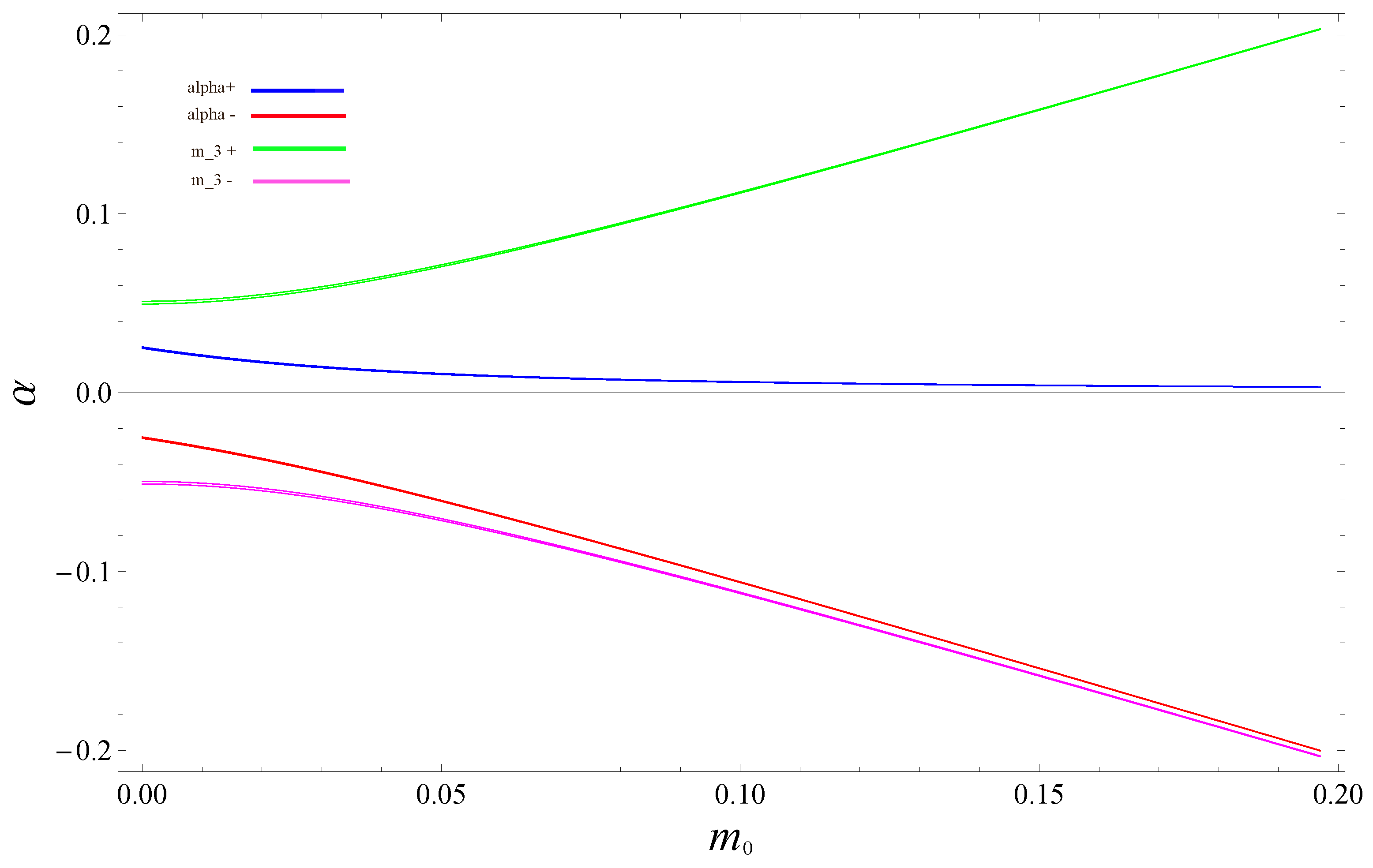
In the first step, we obtain the allowed ranges for the parameters of the neutrino mass matrix along with the perturbation term. We do this by mapping neutrino mass constraints obtained from the experimental data for $\Delta m_{31}^2$ and $\Delta m_{21}^2$ onto our parameter space. In Figure 1, we have shown the limits imposed by $\Delta m_{31}^2$ on the $\alpha$ and $m_0$ parameter space space8 of our model. However, as seen from Equation (5), $\Delta m_{31}^2={(2\alpha +m_0)}^2-m_0^2$. The values of $\alpha$, coming from Equation (23), are

$${\alpha }_{\pm }=-\frac{1}{2}{m}_0\pm \frac{1}{2}\sqrt{m_0^2+|\Delta m_{31}^2|},$$

(23)

where we have denoted these two solutions with upper (plus) and lower (minus) signs. As we see, we always have ${\alpha }_{+}>0$ and ${\alpha }_{-}<0$. In order to visualize the results of Equation (23), in Figure 1 we have plotted $\alpha$ versus $m_0$. We see that we can have $m_3>0$ or $m_3<0$, corresponding to ${\alpha }_{+}$ and ${\alpha }_{-}$, respectively. The range of $m_0$ is very impressible and important because when $m_0>0.197$ then we get ${\alpha }_{+}\to 0$ which yields $m_3^{+}\to m_0$ and ${\alpha }_{-}\to -m_0$ which yields $m_3^{-}\to -m_0$. Such that for both of the cases, the results are unacceptable by comparing with the experimental data. The interesting point is that these results show that the physical mass spectrum is identical for both cases, the green and magenta curves, corresponding to $m_3^{+}$ and $m_3^{-}$ respectively. These curves are symmetric about the $m_0$ axis which is implying phase choice for the $m_3$s, as it is seen in

Table 2. The available experimental data for neutrinos for the case of normal mass hierarchy and the predictions of our model. These predictions are obtained from our parameters as shown in Equation (24).

Parameter	bfp ($\pm 1\mathit{\sigma }$)	Predictions of Our Model
$\Delta m_{21}^2\left({10}^{-5}{\mathrm{eV}}^2\right)$	(7.30–7.72)	(7.43–7.49)
$\Delta m_{31}^2\left({10}^{-3}{\mathrm{eV}}^2\right)$	(2.52–2.57)	(2.40–2.52)
$\delta$	172${}^{\circ }$–218${}^{\circ }$	$({21.48}^{\circ }$–92.29${}^{\circ })\lesssim \delta \lesssim ({267.71}^{\circ }$–338.52${}^{\circ })$
$|J|$	…	≲(0.012–0.035)
masses	…	$m_1\approx$ (0–0.197) $\mathrm{eV},$
		$\langle m_{{\nu }_e}\rangle \approx$ (0.00386–0.20162) eV
	…	$|m_2|\approx$ (0.00862–0.19719) eV, $\varphi \approx ({2.6}^{\circ }$–89.98${}^{\circ })$
		$\langle m_{{\nu }_{\mu }}\rangle \approx$ (0.02737–0.20243) eV
	…	$m_{3\mp }\equiv |m_3|\approx$ (0.0490–0.2033) $\mathrm{eV},$
		$\langle m_{{\nu }_{\tau }}\rangle \approx$ (0.02743–0.20248) eV
$\rho$ and $\sigma$	…	$m_3<0$, $\rho \lesssim -({1.3}^{\circ }$–44.99${}^{\circ })$, $\sigma \lesssim ({88.70}^{\circ }$–45.01${}^{\circ })$
		$m_3>0$, $\rho =\sigma \lesssim -({1.3}^{\circ }$–44.99${}^{\circ })$
$\langle m_{{\nu }_{\beta \beta }}\rangle$	…	$\langle m_{{\nu }_{\beta \beta }}\rangle \approx$ (0.0028–0.12) eV

. Namely, the Majorana phases are different for each case. Hence $|m_3^{+}|=|m_3^{-}|$, and the value of $m_3$s in both case is the same. Naturally, the physics in the perturbation matrix elements does not depend on the chosen solution. We can see no reason to prefer either specific solution. For both values of $\alpha$, our model has normal hierarchy, the same result as in [42].

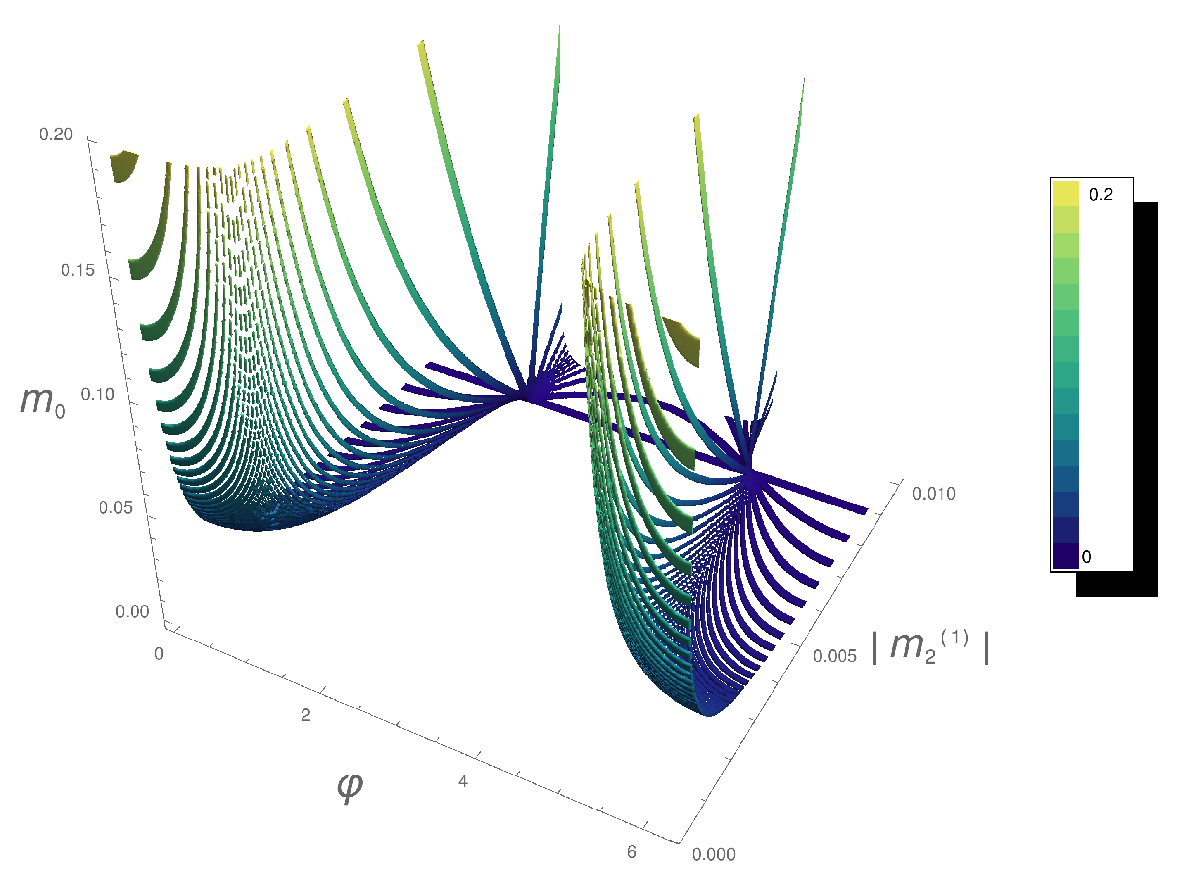
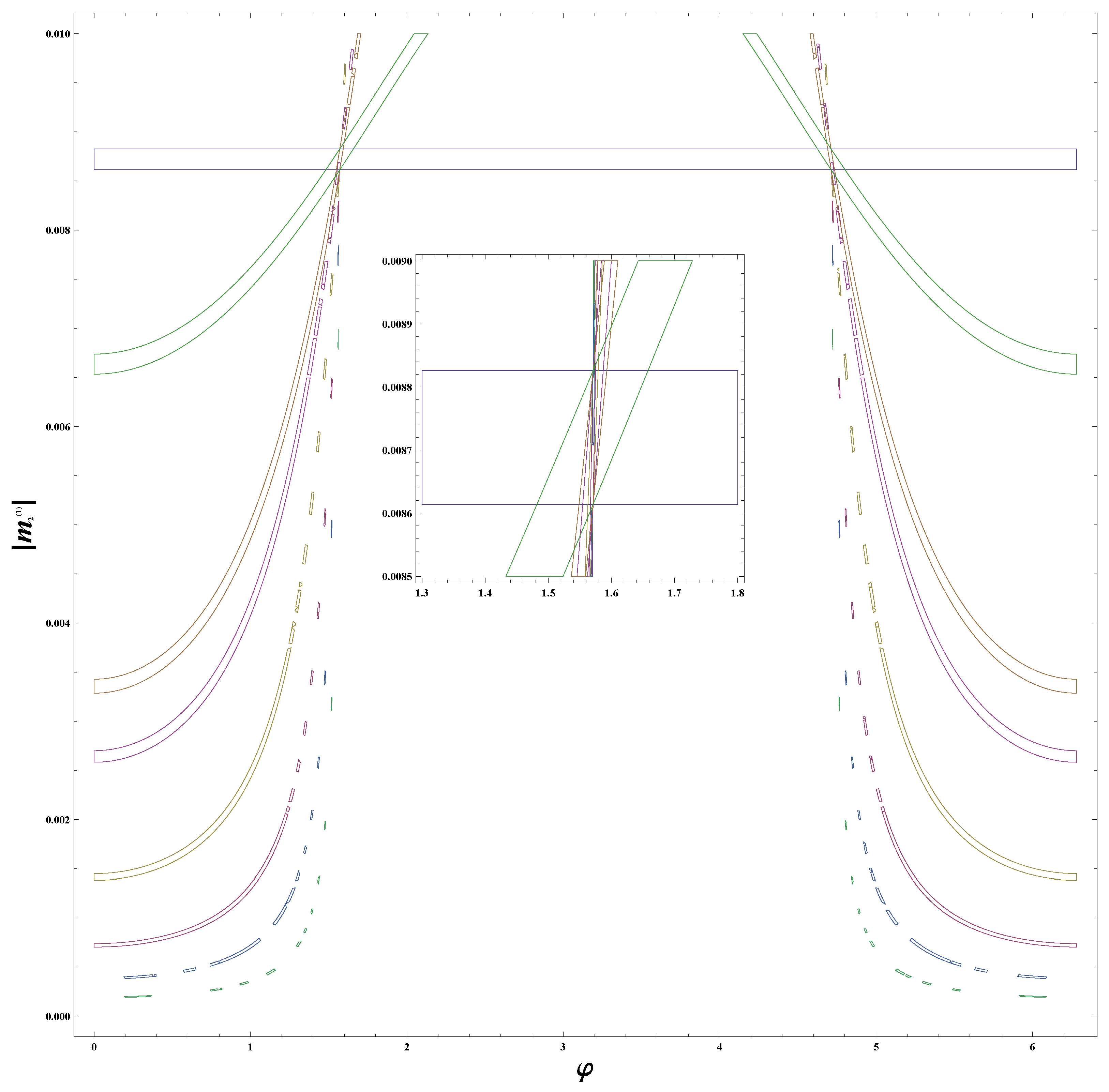
In Figure 2 we have plotted the overlap of $\Delta m_{21}^2$, by using Equations (5) and (19), $\Delta m_{21}^2={|m_2^{\left(1\right)}|}^2+2m_0{m}_2^{\left(1\right)}cos\phi$ with the results obtained in our model along with the allowed ranges of $m_0$ onto the $|m_2^{\left(1\right)}|$ and $\phi$ perturbation parameter space in comparison with experimental data. In Figure 2, each colored curve implies a value of $m_0$ in the equation $\Delta m_{21}^2$ in our model. All these curves overlap with each other in a narrow area in the plane of $|m_2^{\left(1\right)}|$ and $\phi$. Therefore, in Figure 3, we have depicted the contour plot of Figure 2 such that we could clearly show the boundaries of $|m_2^{\left(1\right)}|$ and $\phi$. Our results for the mass matrix parameters are given by

$$\begin{array}{}& \hfill m_0& \approx & (0--0.197)\mathrm{eV},\hfill & \hfill {\alpha }_{-}& \approx & -(0.0245--0.2)\mathrm{eV},\hfill & \hfill {\alpha }_{+}& \approx & (0.0245--0.0033)\mathrm{eV},\hfill & \hfill |m_2^{\left(1\right)}|& \approx & (0.00862--0.00883)\mathrm{eV},\hfill \mathrm{(24)}& \hfill \phi & \approx & ({89.98}^{\circ }--{90.10}^{\circ }).\hfill \end{array}$$

Note that the value of $\phi$ in Equation (24) shows that $m_2^{\left(1\right)}$, the solar neutrino mass splitting term, is dominated by its imaginary part. Therefore, due to the allowed range of $\phi$ [according to (24)], the origin of the Majorana phases, $\varphi$ [in Equation (19)], can take large values. This seems to suggest that the Majorana nature of neutrinos can be responsible for a large value of CP violation in nature [51].

We expect that the different nonzero components of the perturbation matrix Equation (17) are roughly of similar order. We may then expect $\epsilon \equiv \frac{m_2^{\left(1\right)}g\left(\eta \right)}{|\Delta m_{31}^2|s_{13}}\sim \mathcal{O}\left(1\right)$, and could predict the order of $sin{\theta }_{13}$ in $\epsilon$. Therefore, by using the order of $\alpha$ and $|m_2^{\left(1\right)}|$ from the previous stage, we obtain $sin{\theta }_{13}\sim \mathcal{O}\left({10}^{-1}\right)$. Moreover, employing Equation (21), and considering only the order of $sin{\theta }_{13}$, we obtained the allowed range of ${sin}^2{\theta }_{23}$:

$${sin}^2{\theta }_{23}=\frac{|U_{23}{|}^2}{1-|U_{13}{|}^2}\approx (0.505--0.549),$$

(25)

which agrees well with the experimental data.

In the second step, we obtain the allowed ranges for $\delta$ and J, the Jarlskog parameter, as in Equation (A4) and for this we must first determine the allowed range of $\eta$. For this we use the expression of $g\left(\eta \right)$ in Equation (15). Recalling $|m_1|-|m_3|<g\left(\eta \right)<|m_1|+|m_3|$, and so $0.049<g\left(\eta \right)<0.400$, we obtain the allowed range of $\eta$ as $|\eta |\lesssim {92.29}^{\circ }$. In the limit $m_0\to 0$, we get $\eta \to \delta$ and $g\left(\eta \right)\to |m_3|$. In order to get the allowed values of $\delta$, we substitute the allowed ranges of $m_0$, $\alpha$ and $\eta$ into the expression associated to $\delta$ in Equation (14). The results are

$$\begin{array}{c}\hfill ({21.48}^{\circ }--{92.29}^{\circ })\lesssim \delta \lesssim ({267.71}^{\circ }--{338.52}^{\circ }),\end{array}$$

(26)

$$\begin{array}{ccc}\hfill |J|& \lesssim & (0.012--0.035).\hfill \end{array}$$

(27)

Not only we have obtained all the parameters of the model [according to (24)], but now we can also make predictions for the masses of the neutrinos as well as the phases, see Equation (28). We emphasize that we have made predictions that correspond to physical quantities for which there is yet no experimental data. These predictions include

$$\begin{array}{}& \hfill m_1& \approx & (0--0.197)\mathrm{eV},\hfill & \hfill |m_2|& \approx & (0.00862--0.19719)\mathrm{eV}\mathrm{and}\varphi \approx ({2.6}^{\circ }--{89.98}^{\circ }),\hfill & \hfill |m_3|& \approx & (0.0490--0.2033)\mathrm{eV},\hfill & \hfill \Delta m_{21}^2& \approx & (7.43--7.49)\times {10}^{-5}\mathrm{eV},\hfill \mathrm{(28)}& \hfill \Delta m_{31}^2& \approx & (2.40--2.52)\times {10}^{-3}\mathrm{eV}.\hfill \end{array}$$

As mentioned, $\varphi$ is the origin of the Majorana phases which is retrieved from the perturbation. We could dispense with the overall phase, $exp\left(i\varphi \right)$, and therefore we would have two phases that appear in the mass eigenvalues shown in Equation (28). As we noted, these phases are not the same for $|m_3|\equiv m_{3\mp }$. Namely, for $m_{3-}$ we have $\rho =(-\frac{\varphi }{2})$ and $\sigma =(\frac{\pi }{2}-\frac{\varphi }{2})$. Whereas, for $m_{3+}$, $\rho =\sigma =(-\frac{\varphi }{2})$. For the Dirac neutrinos, these phases can be removed, and for the Majorana neutrinos, these phases remain as Majorana phases and contribute to CP violation [52]. Therefore, all of our model predictions for Dirac and Majorana neutrinos (but not for Majorana phases in general) are the same, so no case (Dirac or Majorana) differs from the other so far.

As mentioned, in the Appendix A, in the FL setting $m_0\ne 0$, while the magnitude of the lower bound in Equation (28) is about $m_0=0$. These predictions are compatible with the neutrino mass predictions in [42]. However, it is important to note that the results in this work (such as $\Delta m_{21}^2$ and $\Delta m_{31}^2$), established by means of a different approach, fit the experimental data much better than those reported in [42] especially the best fit column in Table 1. In order to compare our methodology and approach to that in [42] and employing the current experimental data, the ratio $\frac{\Delta m_{21}^2}{\Delta m_{31}^2}$ can be considered as an appropriate parameter. For instance, herein we obtain $\frac{\Delta m_{21}^2}{\Delta m_{31}^2}\approx$ (2.97–3.09) ×${10}^{-2}$, which is closer and more consistent with the best fit experimental data, $\frac{\Delta m_{21}^2}{\Delta m_{31}^2}\approx$ (2.99–3.02) ×${10}^{-2}$, than the corresponding result reported in [42]. Namely, the agreement rate using our improved framework regarding the best fit experimental data is about 30 percent better than in [42]. Moreover, in [41], the phenomenological calculations associated to the CP violation case have not been compared with the corresponding experimental data. In Table 2, we have displayed all of the relevant experimental data presented at Table 1 along with the predictions of our model. As is shown in Table 2 we have predictions for some physical quantities for which there are not any experimental data.

In this model, the magnitude of degeneracy associated with the neutrino masses is defined by $\frac{m_3-m_1}{m_3}$. Hence, the limit $m_1\to 0\left(m_3\right)$ means $0\%(100\%)$ degeneracy among the neutrino masses [53]. We should note that by using the allowed ranges of $m_1$ and $m_3$ in Equation (28) the magnitude of degeneracy of the neutrino masses in our model is ≈(0–97%).

For the flavor eigenstates, we can just calculate the expectation values associated to the masses. Therefore, we can use

$$\langle m_{{\nu }_i}\rangle =\sum _{j=1}^3|U_{ij}{|}^2|m_j|,$$

(29)

where $i=e,\mu ,\tau$. Our predictions for these quantities are as follows, $\langle m_{{\nu }_e}\rangle \approx$ (0.00386–0.20162) eV, $\langle m_{{\nu }_{\mu }}\rangle \approx$ (0.02737–0.20243) eV and $\langle m_{{\nu }_{\tau }}\rangle \approx$ (0.02743–0.20248) eV. The Majorana neutrinos can violate lepton number, for example in neutrinoless double beta decay $\left(\beta \beta 0\nu \right)$ [54]. Such a process has not yet been observed and an upper bound has been set for the relevant quantity, i.e., $\langle m_{{\nu }_{\beta \beta }}\rangle$. Results from the first phase of the KamLAND-Zen experiment sets the following constraint $\langle m_{{\nu }_{\beta \beta }}\rangle <$ (0.061–0.165) eV at 90% CL [55]. Our prediction (better than those in [42]) for this quantity is $\langle m_{{\nu }_{\beta \beta }}\rangle \approx$ (0.0028–0.12) eV which is consistent with the result of kamLAND-Zen experiment.

One of the main experimental result is the sum of the three light neutrino masses which has just been reported by the Planck measurements of the cosmic microwave background (CMB) at $95\%$ CL [56] as

$$\sum m_{\nu }<0.12\mathrm{eV}(\mathrm{Plank}+\mathrm{WMAP}+\mathrm{CMB}+\mathrm{BAO}).$$

(30)

In our model, we obtain $\sum m_{\nu }\approx$ (0.058–0.597) eV, which is in agreement with (30).

4. Discussion and Conclusions

In the next stage, we will consider the attendance of a small contribution, which can be obtained by employing the perturbation theory, which generates small parameters in the neutrino mixing component, namely, $U_{13}$, (${\theta }_{13}$ and $\delta$), $\Delta m_{21}^2$ and provides minor amendments to ${\theta }_{12}$ (but not to ${\theta }_{23}$). CP violation will be investigated.

We should emphasize that in our present work, the method for retrieving the minimal perturbation mass matrix is completely different from those present in the literature (see, e.g., [42] and references therein) and it can be considered as a more fundamentally based approach. The distinguishing features of our herein model are: (i) solely from using the third perturbed mass eigenstate and by employing the rules of the perturbation theory, we constructed the minimal perturbation matrix of the basic tribimaximal mixing matrix, producing a modified Friedberg-Lee model. Therefor, it was produced from the rules of perturbation theory.9 (ii) the perturbation mass matrix is simultaneously responsible for the solar neutrino mass splitting and CP nonconservation in the lepton sector. Consequently, due to these two initiatives and distinctive consideration, our modified framework regarding the best fit experimental data is 30 percent better than in [42]. The model is based on the tribimaximal mixing matrix in which the experimental data of mixing angles (except ${\theta }_{13}$) is well approximated. Therefore, by employing the Friedberg-Lee neutrino mass framework, we obtained the tribimaximal structure which led us to produce a mass matrix constrained by the elements of the TBM mixing matrix and the experimental data. The mass matrix thus obtained (unperturbed mass matrix) loses the solar neutrino mass splitting whilst it remains as a magic and symmetric matrix under $\mu -\tau$ symmetry. At this level, by employing perturbation theory, we generate a perturbation matrix which breaks softly both the $\mu -\tau$ symmetry and the magic feature, and consequently causes CP violation.

Our investigation proceeded in two stages [of Section 2]: CP conservation and CP violation. In the first stage, we obtained the elements of the perturbation matrix in a non CP violation case. In this case, the elements of the perturbation matrix are real, and therefore $\delta =0$ while ${\theta }_{13}\ne 0$.

In the second stage, we extended our study to the case of CP violation, and we obtained the complex elements of the perturbation matrix in both the flavor and mass bases. Moreover, (a) We retrieved a realistic mixing matrix with $\delta \ne 0$. However, in this case, the $\mu -\tau$ symmetry is softly broken, but still we have ${\theta }_{23}={45}^{\circ }$. (b) We obtained the solar neutrino mass splitting dominated by an imaginary term. Therefore, the most important corresponding results or claims are: there is a possibility that Majorana neutrinos exist. According to the results of our herein model, the Majorana phases have been given large values. Hence, it could be a justification for the large leptonic CP violation in nature. Therefore, it is more likely that the neutrinos are of the Majorana type.

In order to get valuable predictions concerning neutrino masses, $\delta$, the origin of the Majorana phases and J, we compared the results of our phenomenological model with experimental data. We have shown that how our phenomenological model whether or not is consistent with experimental data. Mapping two sets of experimental data, namely, the allowed ranges of $\Delta m_{21}^2$ and $\Delta m_{31}^2$ onto the allowed region of our parameter space can determine valid values for our parameters. The consistency of experimental data with the allowed ranges of our parameters shows that our model has normal hierarchy. We then predict the perturbation mass matrix and the values of three masses, $m_1\approx$ (0–0.197) eV, $|m_2|\approx$ (0.00862–0.19719) eV, and $m_3\approx \mp$ (0.0490–0.2033) eV. Therefore, the magnitude of degeneracy for neutrino masses at the end of the allowed ranges is about $97\%$. We have shown that the order of $sin{\theta }_{13}$, which is estimated from the order of the mass parameters, is consistent with the experimental data. We also obtain predictions for the CP violation parameters $\delta$, J, $\rho$ and $\sigma$. These are $|\delta |\lesssim ({21.48}^{\circ }$–92.29${}^{\circ })$, $|J|\lesssim$ (0.012–0.035), while the values of the Majorana phases depend on the sign of $m_3$: for $m_3<0$, $\rho \lesssim -({1.3}^{\circ }$–44.99${}^{\circ })$, $\sigma \lesssim ({88.70}^{\circ }$–45.01${}^{\circ })$, while for $m_3>0$, $\rho =\sigma \lesssim -({1.3}^{\circ }$–44.99${}^{\circ })$. Our predictions for the neutrino masses and CP violation parameters could be tested in future experiments such as the upcoming long baseline neutrino oscillation ones. Moreover, our predictions are entirely consistent with the constraints reported by Planck, WP and high L measurements and the KamLAND-Zen experiment [54,56].

In our model, the minimal perturbation matrix was obtained by means of a fundamental process, and not merely added by hand. Therefore, we can claim that the model presented here can be regarded as presenting a more comprehensive scenario. Another important point is that although our predictions are in correspondence with those in [42], we should emphasize that our outcomes (such as $\Delta m_{21}^2$ and $\Delta m_{31}^2$), constitute with the best fit experimental data reported in Table 1. Last and not least to emphasize, the consistency fitting rate concerning the best fit experimental data is about 30 percent more efficient trough the framework introduced in this paper rather than in [42].

Finally, we plan to subsequently proceed and investigate a $6\times 6$ neutrino mass matrix, by using the same methodology, to obtain the corresponding perturbation mass matrix and CP violation.

References

- Eguchi, K. et al. [KamLAND Collaboration] First Results from KamLAND: Evidence for Reactor Antineutrino Disappearance. Phys.Rev. Lett. 2003, 90, 021802. [Google Scholar] [CrossRef] [PubMed]
- Ahn, M.H. et al. [K2K Collaboration] Indications of Neutrino Oscillation in a 250 km Long-Baseline Experiment. Phys. Rev. Lett. 2003, 90, 041801. [Google Scholar] [CrossRef] [PubMed]
- Dwyer, D.A. [Daya Bay Collaboration]. The Improved Measurement of Electron-antineutrino Disappearance at Daya Bay. Nucl. Phys. Proc. Suppl. 2013, 30, 235–236. [Google Scholar]
- Ahmad, Q.R. et al. [SNO Collaboration] Direct Evidence for Neutrino Flavor Transformation from Neutral-Current Interactions in the Sudbury Neutrino Observatory. Phys. Rev. Lett. 2002, 89, 011301. [Google Scholar] [CrossRef] [PubMed]
- de Salas, P.F.; Forero, D.V.; Gariazzo, S.; Martinez-Mirave, P.; Mena, O.; Ternes, C.A.; Tortola, M.; Valle, J.W.F. 2020 global reassessment of the neutrino oscillation picture. J. High Energy Phys. 2021, 2021, 71. [Google Scholar] [CrossRef]
- Schechter, J.; Valle, J.W.F. Neutrino masses in SU(2)⨂U(1) theories. Phys. Rev. D 1980, 22, 2227. [Google Scholar] [CrossRef]
- Fritzsch, H.; Xing, Z.Z. How to Describe Neutrino Mixing and CP Violation. Phys. Lett. B 2001, 517, 363–368. [Google Scholar] [CrossRef]
- Yao, W.M. et al. [Particle Data Group] Review of Particle Physics. J. Phys. G 2006, 33, 1. [Google Scholar] [CrossRef]
- Harrison, P.F.; Perkins, D.H.; Scott, W.G. A Redetermination of the Neutrino Mass-Squared Difference in Tri-Maximal Mixing with Terrestrial Matter Effects. Phys. Lett. B 1999, 458, 79–92. [Google Scholar] [CrossRef]
- Xing, Z.Z. Nearly tri bimaximal neutrino mixing and CP violation. Phys. Lett. B 2002, 533, 85–93. [Google Scholar] [CrossRef]
- He, X.-G.; Zee, A. Some Simple Mixing and Mass Matrices for Neutrinos. Phys. Lett. B 2003, 560, 87–90. [Google Scholar] [CrossRef] [Green Version]
- Ciafaloni, P.; Picariello, M.; Urbano, A.; Torrente-Lujan, E. Toward a minimal renormalizable supersymmetric SU(5) grand unified model with tribimaximal mixing from A4 flavor symmetry. Phys. Rev. D 2010, 81, 016004. [Google Scholar] [CrossRef]
- Frampton, P.H.; Kephart, T.W.; Matsuzaki, S. Simplified renormalizable T′ model for tribimaximal mixing and Cabibbo angle. Phys. Rev. D 2008, 78, 073004. [Google Scholar] [CrossRef]
- Plentinger, F.; Seidl, G.; Winter, W. Group space scan of flavor symmetries for nearly tribimaximal lepton mixing. J. High Energy Phys. 2008, 2008, 077. [Google Scholar] [CrossRef]
- Bazzocchi, F.; Morisi, S.; Picariello, M. Embedding A4 into left-right flavor symmetry: Tribimaximal neutrino mixing and fermion hierarchy. Phys. Lett. B 2008, 659, 628–633. [Google Scholar] [CrossRef]
- Altarelli, G.; Feruglio, F. Tri-Bimaximal Neutrino Mixing, A4 and the Modular Symmetry. Nucl. Phys. B 2006, 741, 215–235. [Google Scholar] [CrossRef]
- Xing, Z.Z. A translational flavor symmetry in the mass terms of Dirac and Majorana fermions. J. Phys. G 2022, 49, 025003. [Google Scholar] [CrossRef]
- He, X.; Zee, A. Minimal modification to tribimaximal mixing. Phys. Rev. D 2011, 84, 053004. [Google Scholar] [CrossRef]
- Brahmachari, B.; Raychaudhuri, A. Perturbative generation of θ13 from tribimaximal neutrino mixing. Phys. Rev. D 2012, 86, 051302. [Google Scholar] [CrossRef]
- Ghosh, G. Non-zero θ13 and δCP phase with A4 Flavor Symmetry and Deviations to Tri-Bi-Maximal mixing via Z2×Z2 invariant perturbations in the Neutrino sector. Nucl. Phys. B 2022, 979, 115759. [Google Scholar] [CrossRef]
- Grinstein, B.; Trott, M. An expansion for neutrino phenomenology. J. High Energy Phys. 2012, 2012, 5. [Google Scholar] [CrossRef] [Green Version]
- King, S.F. Parametrizing the lepton mixing matrix in terms of deviations from tri-bimaximal mixing. Phys. Lett. B 2008, 659, 244–251. [Google Scholar] [CrossRef]
- Pakvasa, S.; Rodejohann, W.; Weiler, T. Unitary Parametrization of Perturbations to Tribimaximal Neutrino Mixing. Phys. Rev. Lett. 2008, 100, 111801. [Google Scholar] [CrossRef] [PubMed]
- Albright, C.H.; Dueck, A.; Rodejohann, W. Possible Alternatives to Tri-bimaximal Mixing. Eur. Phys. J. C 2010, 70, 1099–1110. [Google Scholar] [CrossRef]
- Wilina, P.; Shubhakanta Singh, M.; Nimai Singh, N. Deviations from Tribimaximal and Golden Ratio mixings under radiative corrections of neutrino masses and mixings. arXiv 2022, arXiv:2205.01936. [Google Scholar] [CrossRef]
- Barradas-Guevara, E.; Félix-Beltrán, O.; Gonzalez-Canales, F. Deviation to the Tri-Bi-Maximal flavor pattern and equivalent classes. arXiv 2022, arXiv:2204.03664. [Google Scholar]
- Boudjemaa, S.; King, S.F. Deviations from Tri-bimaximal Mixing: Charged Lepton Corrections and Renormalization Group Running. Phys. Rev. D 2009, 79, 033001. [Google Scholar] [CrossRef]
- Goswami, S.; Petcov, S.T.; Ray, S.; Rodejohann, W. Large Ue3 and Tri-bimaximal Mixing. Phys. Rev. D 2009, 80, 053013. [Google Scholar] [CrossRef]
- Meloni, D.; Plentinger, F.; Winter, W. Perturbing exactly tri-bimaximal neutrino mixings with charged lepton mass matrices. Phys. Lett. B 2011, 699, 354. [Google Scholar] [CrossRef]
- Garg, S.K. Consistency of perturbed Tribimaximal, Bimaximal and Democratic mixing with Neutrino mixing data. Nucl. Phys. B 2018, 931, 469–505. [Google Scholar] [CrossRef]
- Marzocca, D.; Petcov, S.T.; Romanino, A.; Spinrath, M. Sizeable θ13 from the Charged Lepton Sector in SU(5), (Tri-)Bimaximal Neutrino Mixing and Dirac CP Violation. J. High Energy Phys. 2011, 2011, 9. [Google Scholar] [CrossRef]
- Ma, E.; Wegman, D. Nonzero θ13 for neutrino mixing in the context of A(4) symmetry. Phys. Rev. Lett. 2011, 107, 061803. [Google Scholar] [CrossRef] [PubMed] [Green Version]
- Gupta, S.; Joshipura, A.S.; Patel, K.M. Minimal extension of tri-bimaximal mixing and generalized Z2 X Z2 symmetries. Phys. Rev. D 2012, 85, 031903. [Google Scholar] [CrossRef]
- Adhikary, B.; Brahmachari, B.; Ghosal, A.; Ma, E.; Parida, M.K. A4 symmetry and prediction of Ue3 in a modified Altarelli-Feruglio model. Phys. Lett. B 2006, 638, 345–349. [Google Scholar] [CrossRef]
- Ma, E. Near Tribimaximal Neutrino Mixing with Δ(27) Symmetry. Phys. Lett. B 2008, 660, 505–507. [Google Scholar] [CrossRef]
- Haba, N.; Takahashi, R.; Tanimoto, M.; Yoshioka, K. Tri-bimaximal Mixing from Cascades. Phys. Rev. D 2008, 78, 113002. [Google Scholar] [CrossRef]
- Ge, S.-F.; Dicus, D.A.; Repko, W.W. Residual Symmetries for Neutrino Mixing with a Large θ13 and Nearly Maximal δD, Phys. Rev. Lett. 2012, 108, 041801. [Google Scholar] [CrossRef]
- Araki, T.; Li, Y.F. Q6 flavor symmetry model for the extension of the minimal standard model by three right-handed sterile neutrinos. Phys. Rev. D 2012, 85, 065016. [Google Scholar] [CrossRef]
- Liao, J.; Marfatia, D.; Whisnant, K. Generalized perturbations in neutrino mixing Phys. Rev. D 2015, 92, 073004. [Google Scholar] [CrossRef]
- Garg, S.K. Model independent analysis of Dirac CP violating phase for some well-known mixing scenarios Int. J. Mod. Phys. A 2021, 36, 2150118. [Google Scholar] [CrossRef]
- Friedberg, R.; Lee, T.D. A Possible Relation between the Neutrino Mass Matrix and the Neutrino Mapping Matrix. High Energy Phys.Nucl. Phys. 2006, 30, 591. [Google Scholar]
- Razzaghi, N.; Gousheh, S.S. Neutrino mixing matrix and masses from a generalized Friedberg-Lee model. Phys. Rev. D 2014, 89, 033010. [Google Scholar] [CrossRef]
- Balaji, K.R.S.; Grimus, W.; Schwetz, T. The solar LMA neutrino oscillation solution in the Zee model Phys. Lett. B 2001, 508, 301. [Google Scholar] [CrossRef] [Green Version]
- Lam, C.S. A 2-3 symmetry in neutrino oscillations Phys. Lett. B 2001, 507, 214. [Google Scholar] [CrossRef]
- Grimus, W.; Lavoura, L. Softly broken lepton numbers and maximal neutrino mixing J. High Energy Phys. 2001, 2001, 045. [Google Scholar] [CrossRef]
- Lam, C.S. Magic neutrino mass matrix and the Bjorken–Harrison–Scott parameterization. Phys. Lett. B 2006, 640, 260–262. [Google Scholar] [CrossRef]
- Gautam, R.R.; Kumar, S. Zeros in the magic neutrino mass matrix. Phys. Rev. D 2016, 94, 036004. [Google Scholar] [CrossRef]
- Schiff, L.I. Quantum Mechanics, 3rd ed.; McGraw-Hill: New York, NY, USA, 1968. [Google Scholar]
- Xing, Z.-Z. A Shift from Democratic to Tri-bimaximal Neutrino Mixing with Relatively Large θ13. Phys. Lett. B 2011, 696, 232–236. [Google Scholar] [CrossRef]
- Jarlskog, C. Commutator of the Quark Mass Matrices in the Standard Electroweak Model and a Measure of Maximal CP Nonconservation. Phys. Rev. Lett. 1985, 55, 1039. [Google Scholar] [CrossRef]
- Ballett, P.; Pascoli, S.; Turner, J. Mixing angle and phase correlations from A5 with generalised CP and their prospects for discovery. Phys. Rev. D 2015, 92, 093008. [Google Scholar] [CrossRef]
- Fukugita, M.; Yanagida, T. Physics of Neutrinos and Applications to Astrophysics; Springer: New York, NY, USA, 2003. [Google Scholar]
- Haba, N.; Takahashi, R. Constraints on neutrino mass ordering and degeneracy from Planck and neutrino-less double beta decay. Acta Phys. Polon. B 2014, 45, 61–69. [Google Scholar] [CrossRef]
- Wolfenestein, L. Neutrino oscillations in matter. Phys. Rev. D 1978, 17, 2369. [Google Scholar] [CrossRef]
- Gando, Y. [KamLAND-Zen Collaboration]. Neutrinoless double beta decay search with liquid scintillator experiments. arXiv 2018, arXiv:1904.06655. [Google Scholar]
- Aghanim, N. et al. [Planck] Planck 2018 results. Astron. Astrophys. 2020, 641, A6. [Google Scholar]
- Huang, C.S.; Li, T.; Liao, W.; Zhu, S.H. Generalization of Friedberg-Lee symmetry. Phys. Rev. D 2008, 78, 013005. [Google Scholar] [CrossRef] [Green Version]
- Jenkins, E.; Manohar, A.V. Rephasing Invariants of Quark and Lepton Mixing Matrices. Nucl. Phys. B 2008, 792, 187. [Google Scholar] [CrossRef]
- Zralek, M. 50 Years of Neutrino Physics Acta Phys. Pol. B 2011, 41, 2563. [Google Scholar]
- Zyla, P.A. et al. [Particle Data Group] Review of Particle Physics. PTEP 2020, 2020, 083C01. [Google Scholar]
- Xing, Z.Z.; Zhang, H.; Zhou, S. Nearly Tri-bimaximal Neutrino Mixing and CP Violation from mu-tau Symmetry Breaking. Phys. Lett. B 2006, 641, 189. [Google Scholar] [CrossRef]
- Baba, T.; Yasue, M. Correlation between Leptonic CP Violation and mu-tau Symmetry Breaking. Phys. Rev. D 2007, 75, 055001. [Google Scholar] [CrossRef]
- Xing, Z.Z.; Zhang, H.; Zhou, S. Generalized Friedberg-Lee model for neutrino masses and leptonic CP violation from mu-tau symmetry breaking. Int. J. Mod. Phys. A 2008, 23, 3384–3387. [Google Scholar] [CrossRef] [Green Version]
Figure 1.
Allowed range of in parameter space. Two symmetric spaces are associated to and which yield two different results for .
Figure 2.
In this figure, the whole region of the - plane which is allowed by our model along with the allowed range of is shown. Each color curve implies a value of in the rang (0–0.197) eV in the in our model. The overlap region of the experimental values for with our model are two tiny regions. These regions are the semi-symmetry of each other.
Figure 3.
In this figure, the contour plot of Figure 2, the entire region of the - plane with the allowed range of are shown. In the zoomed box we have magnified the right overlap region.