
A Decision Support System to Enhance Electricity Grid Resilience against Flooding Disasters


1
Department of Civil, Construction & Environmental Engineering, San Diego State University, 5500 Campanile Dr, San Diego, CA 92182, USA
2
Department of Electrical & Computer Engineering, San Diego State University, 5500 Campanile Dr, San Diego, CA 92182, USA
*
Author to whom correspondence should be addressed.
Water 2022, 14(16), 2483; https://doi.org/10.3390/w14162483
Submission received: 1 June 2022
/
Revised: 5 August 2022
/
Accepted: 9 August 2022
/
Published: 12 August 2022
(This article belongs to the Section Urban Water Management)
Abstract
:Highlights
- A decision support system framework based on network cost minimization is proposed to divert flood waters from flood-susceptible utility poles, thereby enhancing electricity grid resilience.
- This optimization framework is evaluated in three different watersheds in the United States using state-of-the-art mathematical optimization platforms, i.e., JuMP/Julia interface and the Gurobi solver.
- The results of this proposed optimization framework could provide adequate flood diversion capacity to prevent failure of utility poles.
Abstract
In different areas across the U.S., there are utility poles and other critical infrastructure that are vulnerable to flooding damage. The goal of this multidisciplinary research is to assess and minimize the probability of utility pole failure through conventional hydrological, hydrostatic, and geotechnical calculations embedded to a unique mixed integer linear programming (MILP) optimization framework. Once the flow rates that cause utility pole overturn are determined, the most cost-efficient subterranean pipe network configuration can be created that will allow for flood waters to be redirected from vulnerable infrastructure elements. The optimization framework was simulated using the Julia scientific programming language, for which the JuMP interface and Gurobi solver package were employed to solve a minimum cost network flow objective function given the numerous decision variables and constraints across the network. We implemented our optimization framework in three different watersheds across the U.S. These watersheds are located near Whittier, NC; Leadville, CO; and London, AR. The implementation of a minimum cost network flow optimization model within these watersheds produced results demonstrating that the necessary amount of flood waters could be conveyed away from utility poles to prevent failure by flooding.
1. Introduction
In modern society, the electricity grid is one of the vital cornerstones of socio-economic prosperity. Humans rely on an uninterrupted supply of electricity for an ever-increasing plethora of needs [1]. When these needs are unmet, the consequences are often severe and range from social disruption to loss of property and life.
In many cases, it is not only the socio-economic activity of communities that is affected by electricity grid failures. Studies by [2,3,4] all present similar evidence pointing to sharp increases in mortality risk and disease during periods of blackout. Each of these studies refer to one particularly devastating blackout during 14–15 August 2003 in New York City. During this time, death, illness, and injury greatly increased due to food poisoning, hypothermia, falling, and the inability to contact health care providers. The multitude of adverse effects caused by power outages on communities in the U.S. and around the world is a rapidly evolving field of research with a wide availability of literature.
There was an unfortunate recurrence of disasters (separate from the incident in New York) caused by electricity grid failures in recent years [5]. According to a University of Vermont study [6], from 1984 to 2006, there were 933 reported power outage events in the U.S., most of which were sustained (lasting longer than 5 min), and wind/rain events causing damage to utility poles and other electricity infrastructure was one of the leading causes. U.S. utility companies are legally obligated to disclose to the North American Electric Reliability Corporation (NERC) any electricity grid irregularities and/or disruptions exceeding 300 megawatts (MW) and impacting 50,000 customers or more. During this 22-year period, it was estimated that over 185,000 individuals were without power and adversely affected by power outages caused by wind/rain. It is likely the weather-related figures are underreported because not all weather-related power outages were accurately reported by utility companies to the NERC [5]. Therefore, the actual number of people impacted by weather-related power outages is likely significantly higher.
Another study conducted by the U.S. Department of Energy (DOE), which has its own database of grid disruption occurrences, demonstrates that during an 18-year period (1992–2010), 78% of 1333 recorded sustained grid disruptions were weather-related (severe rain and wind). It is estimated that these disturbances affected over 178 million customers over the course of the 18-year period [5].
In many cases, the vulnerabilities of U.S. electrical infrastructure are only examined and given necessary attention after these disasters occur [7]. Antiquated electrical infrastructure in the U.S. also produced concerns over national security over the past 20 years. Under current circumstances, U.S. infrastructure is divided into sixteen critical, interrelated, and interdependent sectors, including the electricity grid. Therefore, a natural disaster could be sufficient to cripple not only the electricity grid, but other infrastructure sectors as well, according to Hemme [7]. To address these concerns, recent publications proposed cost-efficient MILP frameworks to enhance the resilience of electricity and natural gas elements of microgrids against various types of disturbances, including natural disasters [8,9]. The results of these two studies provide novel approaches for microgrid operators to contend with disturbances based on different simulated outcomes.
The increasing dependence on an aging electricity grid that became significantly less reliable over the past several years [10] and averting potential disaster when elements of this grid (e.g., power poles) fail were the primary motivations for conducting this study.
This paper particularly focuses on increasing electricity grid resilience by mitigating utility pole failure due to flooding. Example illustration of such a failure is presented by McLaughlin showing utility poles failing from flood waters due to heavy rainfall in Sanford, Michigan [11].
To mitigate utility pole failure, each watershed is mathematically modeled as a network, a system of links and nodes, which can be used to find optimal solutions by optimizing cost, ease of use, failure, energy efficiency, etc. All flow networks have three different types of nodes: production, storage, and consumption [12]. Additionally, as seen in Crucitti et al. [13], not all nodes are created equally; they will have varying capacities based on node type and the composition of the network. Specifically, a minimum-cost network flow methodology is used in this study. This approach was selected because network optimization is proven to be effective across a variety of disciplines.
Recently, there were optimization procedures applied to watershed management for pollution control best management practices, e.g., [14,15] and optimal allocation of water inside distribution networks using various techniques. It does not appear as though a minimum cost network flow optimization problem was applied to a stream network inside a watershed to optimally redirect flood waters away from utility poles.
However, in the past several decades, there was much research conducted on water allocation in river basins via network flow programming. One of the earliest network flow algorithms for watershed planning purposes was developed [16]. An “out-of-kilter” algorithm was introduced in 1976 for optimizing a multi-reservoir network for hydropower and water usage along the Trent River in Ontario, Canada [17].
As years went on, optimization models for watershed management became increasingly more sophisticated [18]. Watershed planning and management models underwent significant advancements in the 1980’s and 1990’s, with the introduction of programs, such as MODSIM3. This was a decision support system based on a network optimization model that allowed the City of Fort Collins, Colorado to more efficiently meet water demands [19]. Six years later, a network flow model called KCOM integrated both surface and subterranean water allocation for Kern County, CA, which allowed for thorough and extensive optimization of the water distribution network in the Kern County Water Bank [20].
Although mixed integer linear programming (MILP) is not a recent technique [21], its application in water resources planning and management contributed to important advancements in recent years. Liu et al. [22] used a MILP approach to meet water usage demands and determine the most cost-efficient placement of water resources infrastructure on the Greek Islands of Paros–Antiparos and Syros. Veintimilla-Reyes [23] adopted MILP to a network optimization problem to create a model addressing water accessibility concerns by predicting appropriate amounts of water in reservoirs at different times of the day. Watson [24] demonstrates that several unique optimization objectives must be considered to realize the optimal configuration of sensor placement for safeguarding water distribution networks. Mani et al. [25] proposed a mixed integer linear fractional programming approach in Northern Louisiana to both maximize groundwater usage and minimize reservoir storage capacity using four existing surface water reservoirs. Groundwater usage was further optimized via conjunctive use with the surface water reservoirs.
The optimization of water distribution operations is by no means a new research topic. However, optimal allocation of drinking water became an extremely important consideration in recent years because of the increasing scarcity of potable water. Studies utilizing both linear and non-linear programming [26] were successful in minimizing cost while ensuring drinking water is efficiently and safely transported through networks to where it is most needed [27]. Municipal water distribution systems are also modeled using “multi-period mixed integer linear programming” to find cost-efficient solutions and meet both potable and non-potable consumer needs [28]. A successful, large-scale instance of multi-period mixed integer linear programming in a water distribution system is found in Kuwait, where the model was applied to energy and water co-generation [29].
This study utilizes a MILP optimization framework as a decision support system to alleviate flooding impacts on utility poles that are at risk of failure. Our model for a node receives flood water from the surface and conveys the flow through a network system of pipe to a discharge point. This type of conveyance occurs only at nodes where drainage is occurring.
The methodology proposed in this study aims to create a versatile decision support framework that will redirect flood waters produced from multiple return periods of storms away from flood-susceptible utility poles through a cost-efficient network of subterranean pipes. For each watershed, storm return periods ranging from 2 to 500 years are individually analyzed at each at-risk utility pole to determine which storm return period(s) cause utility pole failure. The techniques used for obtaining peak flow rates in subwatersheds, and subsequently determining results for the utility pole pass/fail analysis, are further elaborated in the methodology section.
Even though the results of this study represent utility pole failure under some of the worst-case scenario storms, the unprecedented role of climate change in causing these types of “rare” storms to occur more frequently is well documented. Recent studies [30,31,32] confirm with overwhelming evidence that there is a connection between climate change and the increasing frequency of more powerful storms recorded in the U.S. in the past few decades. Many of these more intense precipitation events occurred east of the Rocky Mountains [33]. Since more powerful storms are indisputably occurring more often, developing novel approaches to enhance the resilience of utility poles and the electricity grid against extreme events is of paramount importance at the present time. A 100-year storm is the extreme event of interest for this paper.
This paper contains the following structure: First, the anatomy of the minimum-cost network flow model is discussed with respect to each watershed. Then, the methodology is presented for how each of the peak flow rate inputs to the model is obtained. Subsequently, the minimum cost network optimization problem is introduced, and the decision variables, objective function, and constraints are defined. Lastly, an analysis of the results for each study area is discussed and conclusions are drawn based upon the outputs for the model corresponding to each study area.
2. Methodology
2.1. Study Areas and Hydrologic Analyses
The three watersheds in this paper, Whittier, NC; Leadville, CO; and London, AR, were selected because each are located in underserved areas and contain utility poles susceptible to failure during flood events. These watersheds were delineated using U.S. Geological Survey’s (USGS) Streamstats tool and ArcGIS 10.6.1 with publicly available 10 m digital elevation models (DEMs) from USGS. The Archydro add-on for ArcGIS 10.6.1 was used to delineate subwatersheds inside each watershed.
These subwatersheds each have one longest, aggregate flow path (link). Between each link is a node. Therefore, the number of subwatersheds delineated inside of a watershed determines the composition of the surface node-link network that will be inputted into the optimization model.
Stormwater draining into nodes is modeled to be conveyed through pipes extending downward at a vertical slope to connect with larger diameter pipes that will convey the flow to the most downstream node of the network, i.e., the outfall.
The underground network mirrors the surface network, with the pipe extending from drainage nodes connecting the two. Once the model has run, the optimal underground links are selected, and based on projected cost, runoff is calculated for each subwatershed and the calculated flow rates at which the utility poles fail. These criteria function as the basis for the decision support system.
The Whittier, NC watershed spans an area of 390.4 acres (1.58 sq. km) (Figure 1) and drains into the Tuckasegee River. This watershed is comprised of 31 subwatersheds and 4 utility poles susceptible to failure by flooding. The soil in this watershed is predominantly hydrologic type C. Delineation was performed from the utility pole (green dot) located closest to the Tuckasegee River (Figure 1). The nodes labeled in this figure will be used in the model.
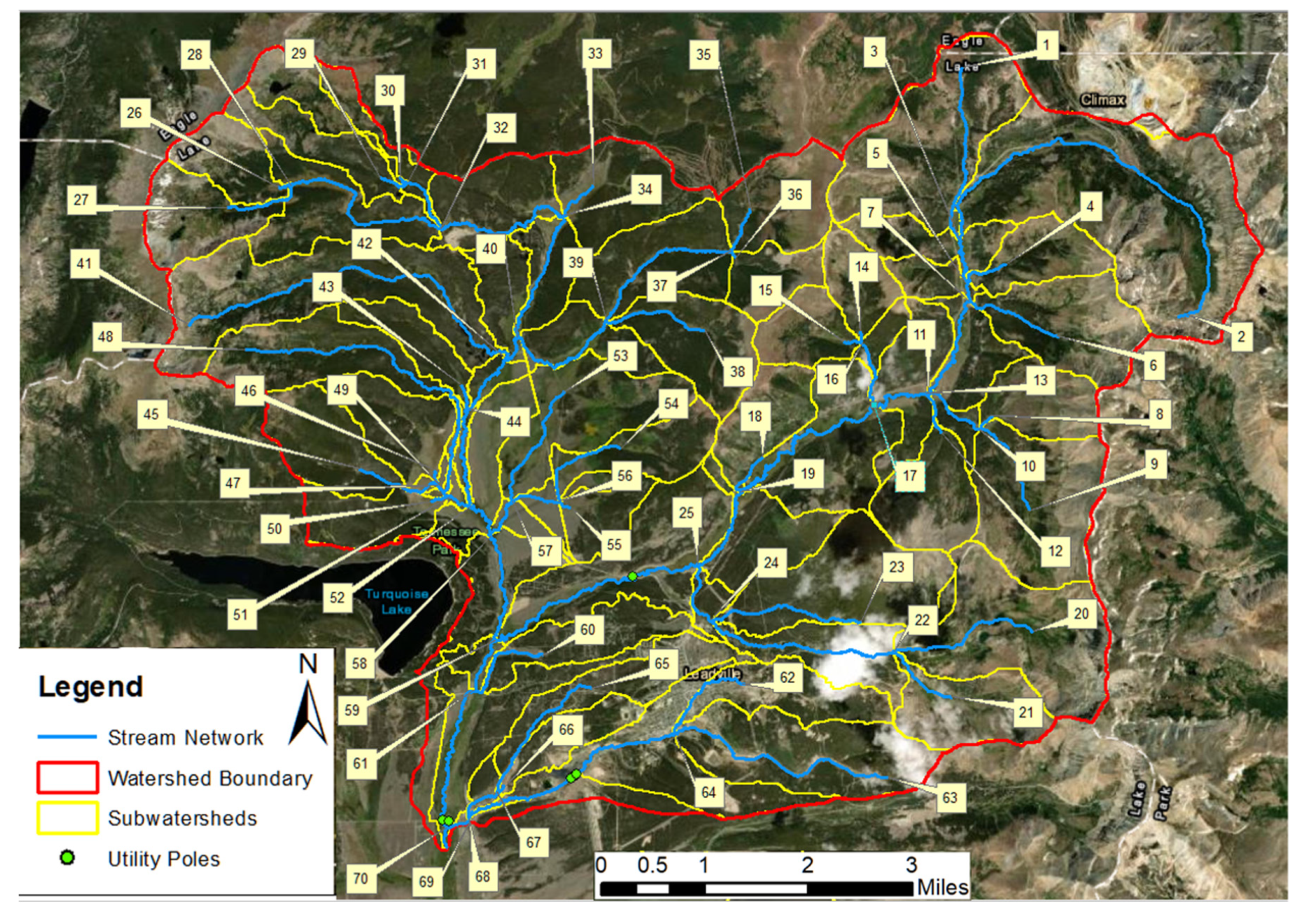
Runoff in the Whittier, NC watershed was calculated using the rational method because each subwatershed has an area (A) sufficiently small (<200 acres) to warrant using this hydrologic method (see Supplementary Information). The second watershed, Leadville, CO, is much larger and is located near Turquoise Lake in Colorado, with an area of 113 sq. miles (292.67 sq. km) and 69 sub watersheds (Figure 2). Two of the watershed’s major streams flow through the town of Leadville. Additionally, there are 6 flood-susceptible utility poles across three locations. This entire watershed stream network ultimately drains into the Arkansas River. Each subwatershed has an area greater than 200 acres and requires the “Natural Resource Conservation Service (NRCS) Curve Number Loss and Dimensionless Unit Hydrograph Method” to accurately calculate the peak flow of each sub watershed (see Supplemental Information). The City of Colorado Springs Drainage Criteria Manual Vol I was used because Leadville and surrounding areas are not densely populated and do not have established hydrology/drainage manuals.
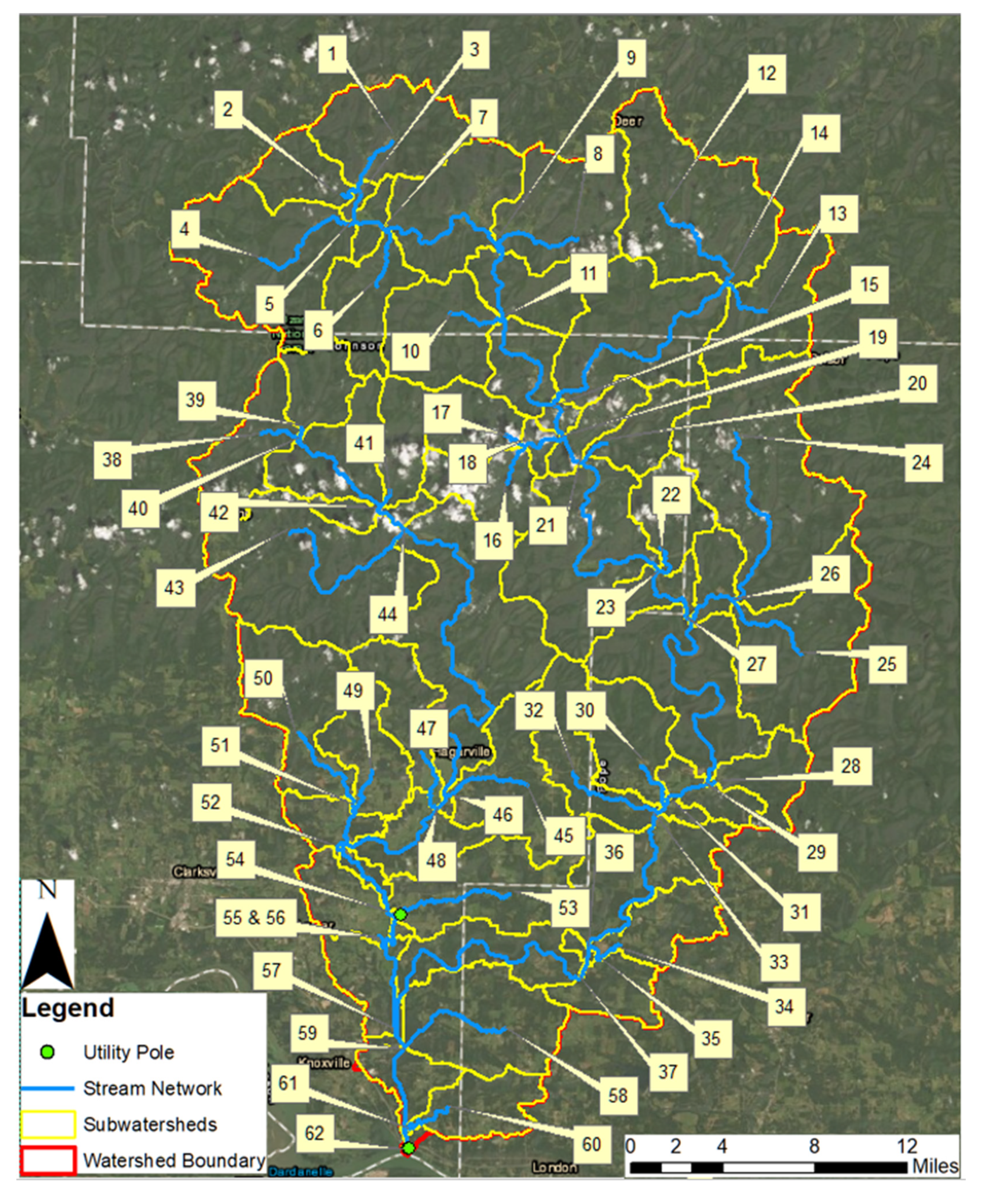
The final watershed, located in Arkansas, discharges into the Arkansas River, near the town of London. Encompassing an area of 537 sq. mile (1390.82 sq. km), this watershed stretches across a portion of the Ozark National Forest and has a major stream flowing through the town of Hagarville (Figure 3). In this watershed, there are only 61 subwatersheds, despite being larger than the Leadville Colorado watershed. There are also 3 utility poles deemed to be flood-susceptible. Similar to the second study area, the NRCS method was used to calculate the runoff for each of the subwatersheds, using nearly the exact same formulae and methodology (see Supplemental Information). The hydrographs developed by the rational and NRCS methods were routed through the river network using the HEC-RAS 5.0.7 software. Cross-sectional areas were derived using the HEC-geoRAS package as an add-on to Arc-GIS based on the digital elevation models for the study areas. HEC-RAS was specifically used to determine the flow depth and velocity at utility pole locations in each watershed.
2.2. Pole Failure Model
The following assumptions were made for all utility poles:
- (1)
- Utility pole–soil interactions can be modeled as a small retaining wall subjected to a passive pressure earth force (Equation (2)), which contributes to the total resisting moment. This total resisting moment opposes the moment created by the force applied by stormwater Equation (1) and the WSE.
- (2)
- The governing drag force formula,was considered to be used to calculate the applied (horizontal) force from stormwater, where V is the velocity of water flow colliding with a utility pole, Cd is the drag coefficient, A is the cross-sectional area, and ρ is the density of water. We also considered the momentum equation for the flow in motion: assuming the velocity is dissipated after hitting the pole (as a conservative assumption), which resulted in more conservative values compared to drag forces, and thus selected in this paper.
- (3)
- (4)
- Full setting depth is determined by the commonly accepted rule, 10% of the utility pole length plus two feet [35].
- (5)
- All utility poles are directly buried in the soil with no embedment foundation, based on observations made in Google Street View.
- (6)
- The version of the Rankine passive earth pressure force of the soil (Equation (11)) was used based on the assumption that the soils in each watershed are predominantly granular [36].
Assumption 6 was confirmed with an online U.S. Department of Agriculture (USDA) Natural Resources Conservation Service (NRCS) Web Soil Survey analysis in areas near the utility poles.
Passive earth pressure exists when a lateral force is causing a retaining wall to move toward the soil [36]. Gamma (γ) is the bulk density of soil and in this study, and is estimated based on the soil texture and observed vegetation around utility poles (Table 1). There are several in situ methods for accurate estimation of soil bulk density [37]. However, these methods are outside the scope of this network optimization research.
Bulk density estimates are around the upper or lower limit based on observed vegetation growth in areas around utility poles. The bulk density values were referenced from an NRCS publication [38].
- (7)
- In Rankine theory, it is assumed that the structure being modeled as a retaining wall is completely vertical and has a smooth surface. Therefore, factors such as wall–soil friction and retaining wall sloping are negligible.
- (8)
- Equation (3) assumes that there is no angle of incline and only takes into consideration the angle of friction. Kp is the Rankine passive pressure coefficient, which can be calculated from the following equation.
- (9)
- Based on [36], it is assumed the resisting force is applied at approximately 2/3 of the utility pole (retaining wall) burial depth (measured from the ground line downward), or a distance 1/3 from the bottom of the utility pole (measured upward).
The angle of friction is determined based on a soil’s grain distribution size, void ratio, surface roughness, and angularity [39]. A proposed regression model [40] calculated an average friction angle for four different types of sand based on stress–displacement performance. The average soil friction angle calculated for group 3 sands was 35°, and this is consistent with values reported in USCS soil friction angle charts [41] and in the USDA publication [39] for sandy, non-cohesive soils.
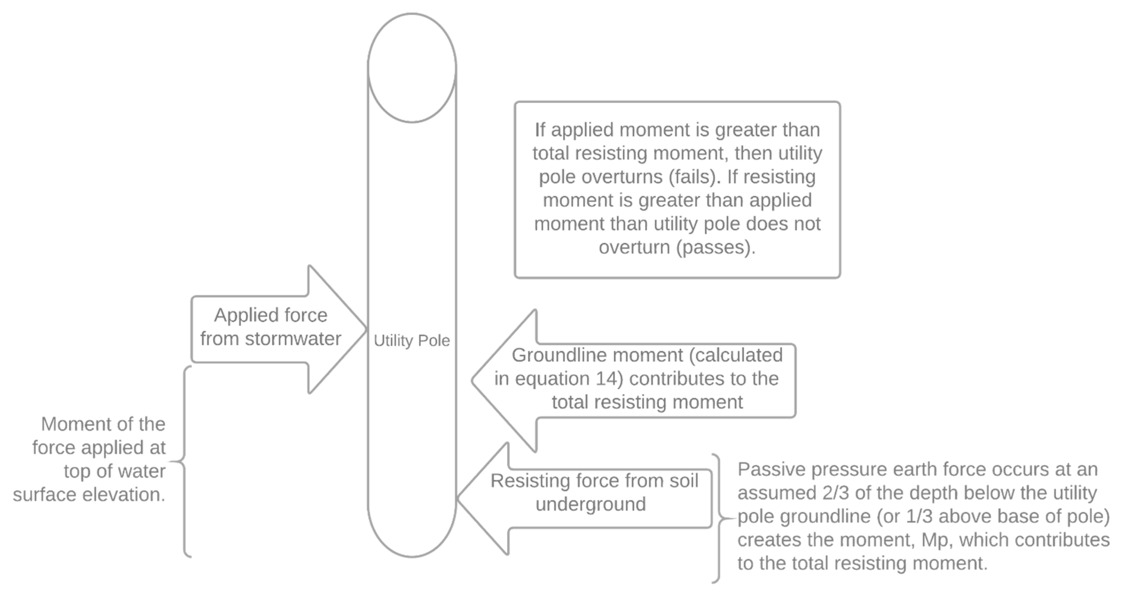
It is assumed that each utility pole in this study will be subjected to an applied moment of stormwater at a depth varying with the storm return period (WSE) and a cumulative resisting moment. This total resisting moment (Mt) is the sum of the maximum allowable moment at the utility pole groundline (Mgl) (Equation (5)) [35] and the product of the passive pressure occurring at a depth of (2/3)H (Mp).
where fs is the fiber stress (psi) of the wood utility pole, according to the American National Standards Institute (ANSI). This value varies based on the class and species of the pole (Table 2). The diameter (d) of the utility pole at the groundline can also be expressed as
where the circumference of the utility pole at groundline (C) is calculated as follows
C0 and C1 are the circumferences of the pole at the top and 6 feet from the bottom, respectively. The total length (L) of the pole has a setting depth (E) associated with it, and the constant 6 denotes 6 ft subtracted from the total length of the pole. Equations (5)–(7) follow the methodology used by Keshavarzian [35].
In Table 2, the southern pine pole species was assumed for all utility poles because that is the species of wood used for most utility poles in North America [42]. Assumed utility pole lengths were estimated from a google street view analysis. A circumference 6 feet from the pole bottom was determined using a circular taper factor of 0.25 in/ft. Setting depth was determined using the 10% of total length plus two feet rule.
Figure 4 depicts the culmination of the hydrostatic and geotechnical calculations. The accumulated flow from each subwatershed along a stream is used to calculate the applied moment on a utility pole. The same calculations were performed for every at-risk utility pole in each of the watersheds. The flow rate causing the applied moment to be equal to the resisting moment is the upper limit of Equation (14), which is discussed in the next subsection.
2.3. Minimum Cost Network Flow Optimization Problem
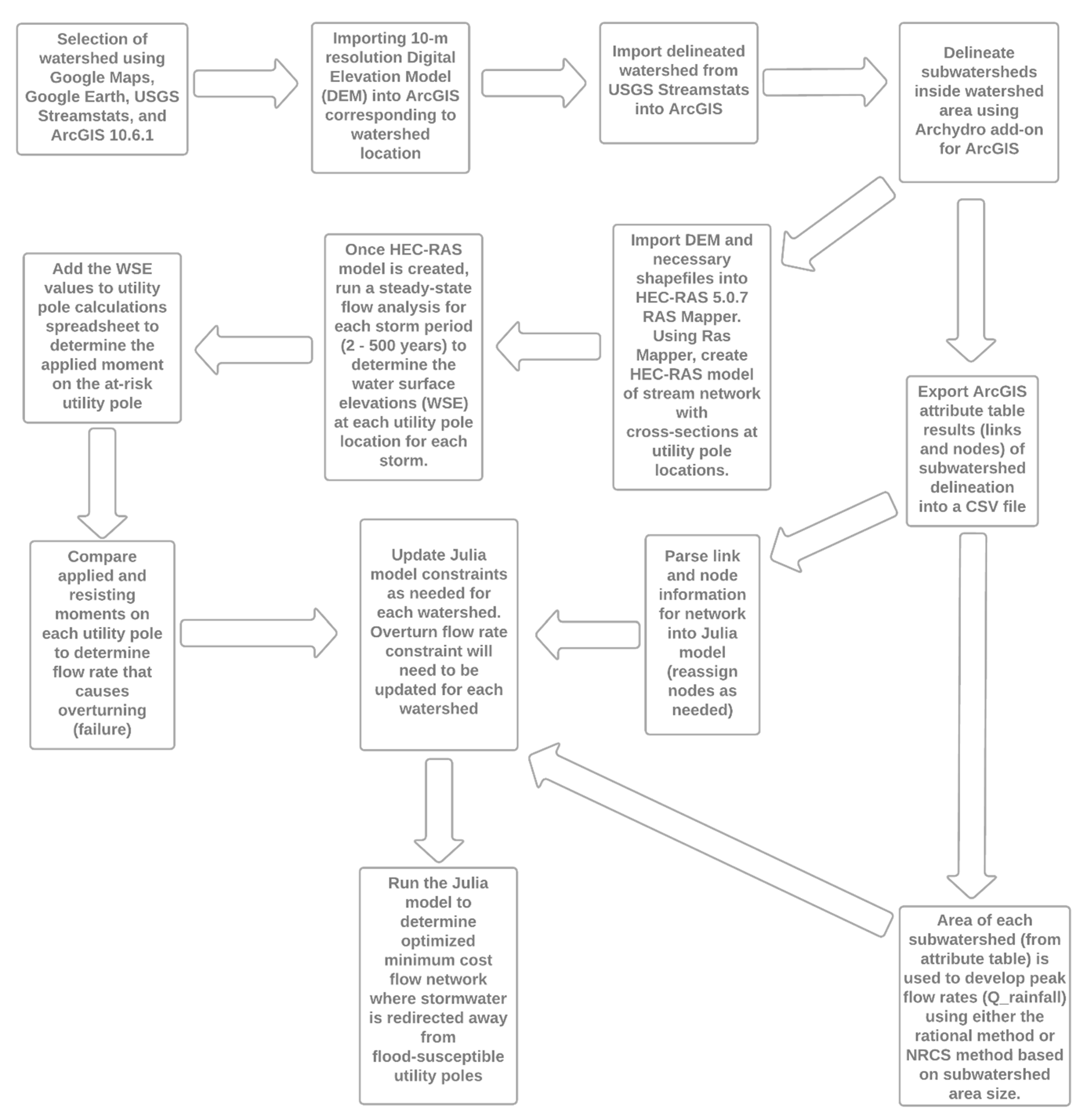
A comprehensive methodology to build and process data for this MILP decision support system are summarized in Figure 5. Performing the hydrostatic and geotechnical calculations assesses whether a utility pole will fail at a given peak flow rate. An approximate water surface elevation (WSE) had to be determined at a cross section at the utility pole location. HEC-RAS 5.0.7 (HEC-RAS) was used to determine the WSEs at utility poles in each watershed.
Flow across any network is governed by costs associated with production, some material in transit across the links, and a series of constraints applying to the links and nodes. Additionally, any optimization problem will consist of an objective function, decision variables, and constraints. This is the core anatomy of a network optimization problem. It is important to note that network optimization problems can be applied to many other facets of life outside of electricity grid design and water resources infrastructure, e.g., [43,44].
Although many solvers exist for optimization problems, [45] suggests that both the Gurobi solver and the JuMP interface are well-suited to MILP problems. To prevent utility pole failure, a minimum cost network flow problem will be established, where each watershed will be treated as a network of links and nodes. Each surface link (segment of stream) occupies one sub watershed and nodes are the vertices on either end of a stream segment. In the underground network, nodes are on either end of nearhorizontal pipes (this term was used to show the contrasts with the vertical drainage elements):
Costi and Costp are the cost of the vertical and horizontal pipe, respectively. Near-horizontal pipes follow the mild slope of the natural terrain. The Manning’s equation was used to calculate the flow capacity of the subterranean pipes network. Links in the subterranean network consist of:
- (1)
- pipe extending vertically downward from surface nodes to connect to horizontal pipe and
- (2)
- horizontal pipe conveying stormwater to the network outfall, or discharge point.
The vertical and horizontal pipes comprise the underground network. The optimal underground network is the target output of this model.
Ui is a binary decision variable that functions as either 0 or 1, depending on the existence of drainage at a node. Up is a second binary decision variable, that dictates if there will be flow through an underground pipe or not. Flow rate units were calculated in cubic feet per second (cfs).
Equation (8) is the objective function for the minimum cost network flow problem and is subject to a series of constraints that define the feasible decision space. Equation (9) is for surface links that do not contain utility poles.
Qhydraulic capacity is expressed as the upper limit of Equations (10) and (11), and can be used to size the vertical pipes connected to nodes and the horizontal underground pipes that will be used in the model. There are two conservation of flow constraints, one for surface network nodes and another for nodes in the underground network. Both of the conservation of flow constraints (Equations (12) and (13)) incorporate the Qstream, Qdrained, and Qpipe decision variables seen above. Qstream refers to only the surface stream network. Qdrained is used in Equations (12) and (13) and is denoted in the surface network (Equation (12)) as Qdrained(i) to determine the amount of stormwater to be conveyed into the vertical pipe at certain surface nodes so that utility pole failure is mitigated. In Equation (13), Qdrained(p) signifies stormwater in the underground network being conveyed downward through a vertical pipe to the horizontal pipe. Once Qdrained(p) reaches the horizontal pipe, it becomes Qpipe, and is carried to the underground network’s node of discharge (outfall).
It should be noted that Qrainfall becomes Qstream in every subwatershed and flows into every downstream subwatershed.
Equation (12) is used to balance the network nodes on the surface and Equation (13) balances the subterranean nodes. These two equations function in tandem with one another to connect the surface stream network to the vertical and horizontal pipes comprising the underground network. Essentially, the left side of Equations (12) and (13) are stating that the flow of stormwater exiting a node at a link is subtracted by the flow of stormwater entering a node in the subsequent link and is equal to the net amount of stormwater at a particular node. Therefore, Equations (12) and (13) are referred to as node balance equations, or flow conservation constraints.
Discharge represents stormwater leaving the network at a specified node both at the surface (Discharge(i)) and in the underground pipe network (Discharge(p)). For all networks in this study, discharge only occurs at the downstream terminal node.
Lastly, there are additional constraints for each of the utility pole locations, dictating that flow in a stream segment corresponding to a utility pole location cannot exceed the flow rate that would cause utility pole failure (overturning). Each of these constraints will take the following form and are crucial to the entire decision support system because they allow the model to decide how much stormwater to allocate to the underground network.
Once water surface elevations were determined for each storm return period via a steady-state flow analysis in HEC-RAS, they were used to compute the moment being applied on the utility pole of interest. From there, the flow rate at which the utility pole failed is inferred. This flow rate is the upper limit of Equation (14).
3. Results
The methods enumerated above were applied to each watershed to test the model’s efficacy on networks of different size and composition. The results of the calculations for one utility pole in the Whittier, NC watershed (Table 3) are used as an example to illustrate a typical analysis for every utility pole. In Table 4, Table 5 and Table 6, the hydraulic capacity is the output of the model. “Drainage Capacity Recommended” is the amount of drainage occurring at a node for the model to reach the optimal solution. “Underground Pipe Flow” is the sum of surface drainage at a node and drainage occurring at any upstream nodes conveyed to that node.
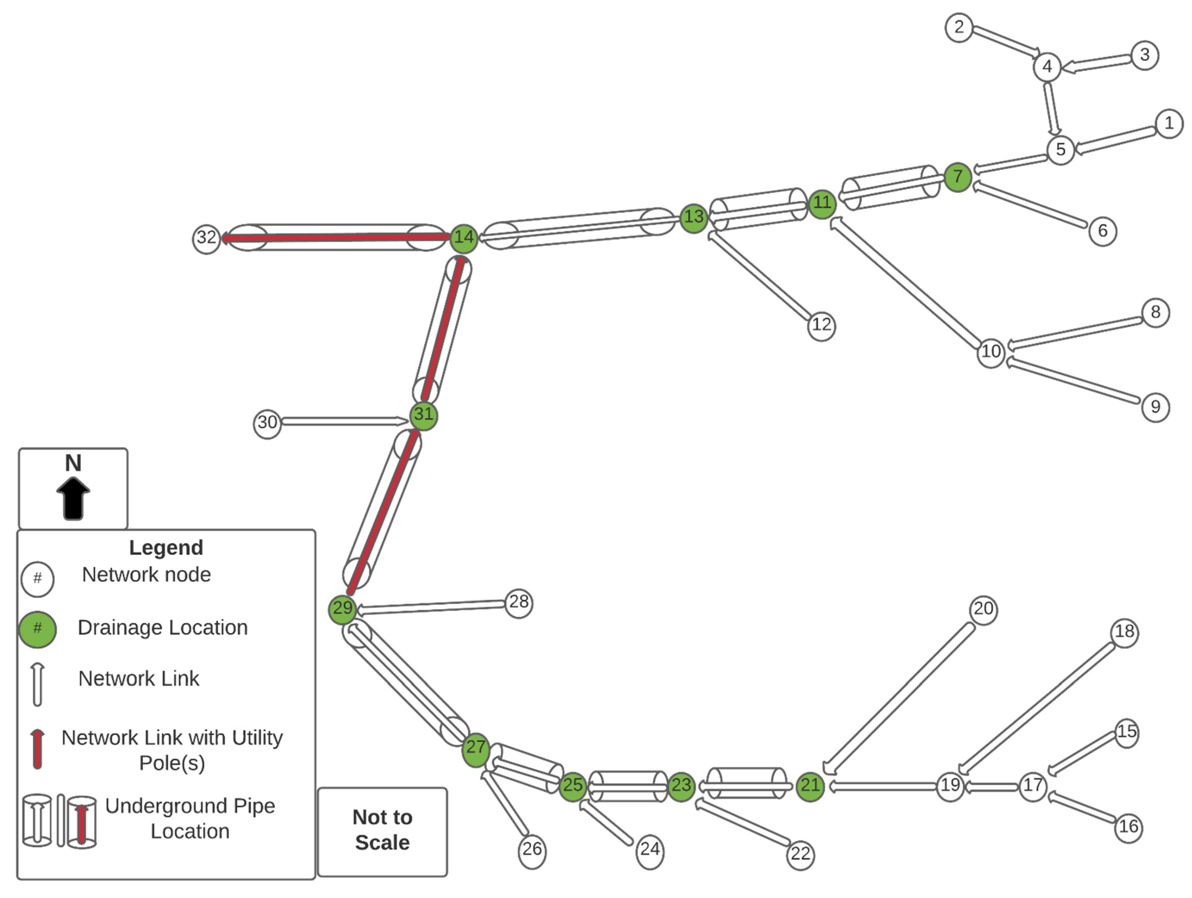
Figure 6, Figure 7 and Figure 8 were designed to be used as visual aids to interpret the data outputs in Table 4, Table 5 and Table 6, where locations of utility poles (red arrows) and underground pipe are clearly denoted. The nodes and links in Figure 6, Figure 7 and Figure 8 can also be referenced to exact locations within each watershed by using Figure 2, Figure 3 and Figure 4.
Some of the WSEs in Table 3 are high because the Whittier, NC watershed has a steep average slope and there are well-defined channels towards the confluence of the watershed’s streams. These are where the flood-susceptible utility poles are located (Figure 6) and where cross-sections were taken in HEC-RAS.
4. Discussions and Conclusions
The model is behaving as expected for each of the watersheds. Sufficient drainage is occurring at nodes (drainage capacity recommended) to mitigate utility pole failure. In the Whittier, NC watershed, this will allow successively larger underground pipes to convey flood water away from utility poles. The hydraulic capacities reported in Table 4 were a result of flow rates from the 100-year storm and are appropriate for feasible pipe diameters. In the Leadville, CO and London, AR watersheds, peak flow rates for the 100-year storm were much higher due to larger subwatershed areas. Therefore, the model is reporting large hydraulic capacities for node drainage and underground pipe flow (Table 5 and Table 6) that are not conducive to feasible pipe diameters. This means that utility poles in the Leadville, CO and London, AR watersheds are at great risk of failure during severe flooding events, and to mitigate this failure using the current framework would require unreasonably large vertical and horizontal pipes. To resolve this issue, one can adopt alternative measures, including changes in the utility distribution line types (e.g., installing lines underground), which is beyond the scope of our particular study.
Based on the outputs of the model in Table 5 and Table 6, it is recommended that any future versions of this study delineate smaller subwatersheds inside the two larger watersheds. Smaller subwatersheds would result in lower peak flow rates and a larger network. Therefore, a more robust decision support system would also be created where the hydraulic capacity results would be conducive to feasible pipe diameters.
The present decision support system could be further strengthened by adding more decision variables. An additional decision variable could be added at certain nodes for above-ground hydraulic structures, such as trapezoidal channels. These channels can convey high peak flow rates and would be feasible in the Leadville, CO and London, AR watersheds due to existing lakes. The channels’ conveyance of high peak flow rates would lessen the load on the optimal underground pipe network. In Table 4, Table 5 and Table 6, many of the node drainage values repeat. This is because the model is maximizing the amount of drainage occurring at nodes, so the optimized network has the fewest possible pipes with minimum deployment cost.
Nearly all the utility poles analyzed for the 100-year storm were projected to fail based on the calculations (refer to Table 3 for calculation result template). However, the utility pole at link 53.54 in the London, AR watershed passed. As seen in Figure 8, the model deemed drainage to be unnecessary at node 53 because the constraint summarized in Equation (14) was not violated. This was due to a low peak flow rate in the link’s corresponding subwatershed.
Future studies should consider a more thorough methodology for flood-susceptible utility pole identification. Alam [46] devised a methodology to determine utility pole vitality through photography from unmanned aerial vehicles (UAVs) and computation of “computer vision-based” angles of inclination. Post-computation, utility poles with angles of inclination reflecting an unhealthy condition (>10°) can be identified. After identification, the framework introduced in this study could be applied so that any failure due to flooding is mitigated.
Photography from UAVs could also strengthen the techniques proposed in this study. There are commercially available software packages (Ansys Workbench and O-Calc Pro Line Design) that use photogrammetry to determine accurate measurement of objects. Utility pole photography could be analyzed in either of these programs to determine more accurate measurements of the diameter, circumference, and length of the pole, which factor into calculations for the total resisting moment. A more accurately calculated resisting moment will produce an even more reliable analysis of utility pole failure.
The results of this MILP optimization framework, using the Gurobi solver inside the JuMP interface, are encouraging because the model demonstrated the ability to successfully redirect flood waters from at-risk utility poles. Therefore, the novel methodology proposed in this study can alleviate flood vulnerabilities in the U.S. electricity grid and abroad.
Supplementary Materials
Author Contributions
H.D. Formulating the research questions and data collection. M.V. Implementing the optimization model and writing the draft manuscript. S.D.M. Supervising the analyses and reviewing the manuscript and visualizations. All authors have read and agreed to the published version of the manuscript.
Funding
The work submitted for publication is un-funded.
Institutional Review Board Statement
Not applicable.
Informed Consent Statement
Not applicable.
Data Availability Statement
All data, models, or code that support the findings of this study are available from the corresponding author upon reasonable request.
Conflicts of Interest
The submitted article represents an original scientific work that has not been published and is not under consideration for publication elsewhere. All works referred to in the article have been acknowledged by proper citation, and there is no real or apparent conflict of interests in its content. There is no financial or non-financial interests that are directly or indirectly related to the work submitted for publication. The work submitted for publication is un-funded.
References
- Pant, R.; Thacker, S.; Hall, J.W.; Alderson, D.; Barr, S. Critical infrastructure impact assessment due to flood exposure. J. Flood Risk Manag. 2018, 11, 22–33. [Google Scholar] [CrossRef]
- Anderson, G.B.; Bell, M.L. Lights Out: Impact of the August 2003 Power Outage on Mortality in New York, NY. Epidemiology 2012, 23, 189–193. [Google Scholar] [CrossRef] [PubMed]
- Klinger, C.; Owen Landeg, V.M. Power outages, extreme events and health: A systematic review of the literature from 2011–2012. PLoS Curr. 2014, 6, 14–27. [Google Scholar] [CrossRef]
- Marx, M.A.; Rodriguez, C.V.; Greenko, J.; Das, D.; Heffernan, R.; Karpati, A.M.; Mostashari, F.; Balter, S.; Layton, M.; Weiss, D. Diarrheal illness detected through syndromic surveillance after a massive power outage: New York City, August 2003. Am. J. Public Health 2006, 96, 547–553. [Google Scholar] [CrossRef] [PubMed]
- Campbell, R.J.; Lowry, S. Weather-Related Power Outages and Electric System Resiliency; CRS Report for Congress: Washington, DC, USA, 2012. [Google Scholar]
- Hines, P.; Apt, J.; Talukdar, S. Trends in the history of large blackouts in the United States. In Proceedings of the 2008 IEEE Power and Energy Society General Meeting-Conversion and Delivery of Electrical Energy in the 21st Century, Pittsburgh, PA, USA, 20–24 July 2008; pp. 1–8. [Google Scholar]
- Hemme, K. Critical infrastructure protection: Maintenance is national security. J. Strateg. Secur. 2015, 8, 25–39. [Google Scholar] [CrossRef]
- Manshadi, S.; Khodayar, M. Resilient Operation of Multiple Energy Carrier Microgrids. IEEE Trans. Smart Grid 2015, 6, 2283–2292. [Google Scholar] [CrossRef]
- Manshadi, S.; Khodayar, M. Preventive reinforcement under uncertainty for islanded microgrids with electricity and natural gas networks. J. Mod. Power Syst. Clean Energy 2018, 6, 1223–1233. [Google Scholar] [CrossRef]
- Li, Z.; Guo, J. Wisdom about age [aging electricity infrastructure]. IEEE Power Energy Mag. 2006, 4, 44–51. [Google Scholar]
- McLaughlin, K. Photos and Videos Show the Destruction after 2 Dams Collapsed in Michigan, Threatening a Town with 9 Feet of Flooding. Insider. Available online: https://www.insider.com/photos-videos-show-michigan-dam-collapse-destruction-2020-5 (accessed on 20 May 2020).
- Turnquist, M.; Vugrin, E. Design for resilience in infrastructure distribution networks. Environ. Syst. Decis. 2013, 33, 104–120. [Google Scholar] [CrossRef]
- Crucitti, P.; Latora, V.; Marchiori, M. Model for cascading failures in complex networks. Phys. Rev. E 2004, 69, 045104. [Google Scholar] [CrossRef]
- Maringanti, C.; Chaubey, I.; Arabi, M.; Engel, B. Application of a Multi-Objective Optimization Method to Provide Least Cost Alternatives for NPS Pollution Control. Environ. Manag. 2011, 48, 448–461. [Google Scholar] [CrossRef] [PubMed]
- Muleta, M.K.; Nicklow, J.W. Evolutionary algorithms for multiobjective evaluation of watershed management decisions. J. Hydroinformatics 2002, 4, 83–97. [Google Scholar] [CrossRef]
- Evenson, D.E.; Moseley, J.C. Simulation/Optimization Techniques for Multi-Basin Water Resource Planning1. J. Am. Water Resour. Assoc. 1970, 6, 725–736. [Google Scholar] [CrossRef]
- Sigvaldson, O.T. A simulation model for operating a multipurpose multireservoir system. Water Resour. Res. 1976, 12, 263–278. [Google Scholar] [CrossRef]
- Ilich, N. Limitations of Network Flow Algorithms in River Basin Modeling. J. Water Resour. Plan. Manag. 2009, 135, 48–55. [Google Scholar] [CrossRef]
- Labadie, J.W.; Bode, D.A.; Pineda, A.M. Network Model for Decision Support in Municipal Raw Water Supply. J. Am. Water Resour. Assoc. 1986, 22, 927–940. [Google Scholar] [CrossRef]
- Andrews, E.S.; Chung, F.I.; Lund, J.R. Multilayered, Priority—Based Simulation of Conjunctive Facilities. J. Water Resour. Plan. Manag. 1992, 118, 32–53. [Google Scholar] [CrossRef]
- Bixby, R. A Brief History of Linear and Mixed-Integer Programming Computation. Doc. Math. 2012, 2012, 107–121. [Google Scholar]
- Liu, S.; Konstantopoulou, F.; Gikas, P.; Papageorgiou, L.G. A mixed integer optimisation approach for integrated water resources management. Comput. Chem. Eng. 2011, 35, 858–875. [Google Scholar] [CrossRef]
- Veintimilla-Reyes, J.; Cattrysse, D.; De Meyer, A.; Van Orshoven, J. Mixed integer linear programming (MILP) approach to deal with spatio-temporal water allocation. Procedia Eng. 2016, 162, 221–229. [Google Scholar] [CrossRef]
- Watson, J.-P.; Greenberg, H.J.; Hart, W.E. A Multiple-Objective Analysis of Sensor Placement Optimization in Water Networks. Crit. Transit. Water Environ. Resour. Manag. 2004, 5, 1–10. [Google Scholar]
- Mani, A.; Tsai, F.T.-C.; Paudel, K.P. Mixed Integer Linear Fractional Programming for Conjunctive Use of Surface Water and Groundwater. J. Water Resour. Plan. Manag. 2016, 142, 04016045. [Google Scholar] [CrossRef]
- Carini, M.; Maiolo, M.; Pantusa, D.; Chiaravalloti, F.; Capano, G. Modelling and optimization of least-cost water distribution networks with multiple supply sources and users. Ric. Mat. 2018, 67, 465–479. [Google Scholar] [CrossRef]
- Bieupoude, P.; Azoumah, Y.; Neveu, P. Optimization of drinking water distribution networks: Computer-based methods and constructal design. Comput. Environ. Urban Syst. 2012, 36, 434–444. [Google Scholar] [CrossRef]
- Ghelichi, Z.; Tajik, J.; Pishvaee, M.S. A novel robust optimization approach for an integrated municipal water distribution system design under uncertainty: A case study of Mashhad. Comput. Chem. Eng. 2018, 110, 13–34. [Google Scholar] [CrossRef]
- Alqattan, N.A. A Multi-Period Mixed Integer Linear Programming Model for Desalination and Electricity Co-generation in Kuwait. Graduate Thesis, USF Tampa, Tampa, FL, USA, 2014. [Google Scholar]
- Lubchenco, J.; Hayes, J. A better eye on the storm. Sci. Am. 2012, 306, 68–73. [Google Scholar] [CrossRef]
- Teegavarapu, R.S. Climate variability and changes in precipitation extremes and characteristics. In Sustainable Water Resources Planning and Management Under Climate Change; Springer: Berlin/Heidelberg, Germany, 2017; pp. 3–37. [Google Scholar]
- Trenberth, K.E. Changes in precipitation with climate change. Clim. Res. 2011, 47, 123–138. [Google Scholar] [CrossRef]
- Groisman, P.Y.; Knight, R.W.; Karl, T.R. Changes in intense precipitation over the central United States. J. Hydrometeorol. 2012, 13, 47–66. [Google Scholar] [CrossRef]
- Davisson, M.; Prakash, S. A Review of Soil-Pole Behavior; Highway Research Record (39); Highway Research Board: Washington, DC, USA, 1963. [Google Scholar]
- Keshavarzian, M. Self-supported Wood Pole Fixity at ANSI Groundline. Pract. Period. Struct. Des. Constr. 2002, 7, 147–155. [Google Scholar] [CrossRef]
- Das, B.M. Principles of Foundation Engineering, 8th ed.; Cengage Learning: Boston, MA, USA, 2016; pp. 593–645. [Google Scholar]
- Al-Shammary, A.A.G.; Kouzani, A.Z.; Kaynak, A.; Khoo, S.Y.; Norton, M.; Gates, W. Soil Bulk Density Estimation Methods: A Review. Pedosphere 2018, 28, 581–596. [Google Scholar] [CrossRef]
- USDA NRCS. (n.d.). Soil Bulk Density/Moisture/Aeration. USDA-NRCS. Available online: https://www.nrcs.usda.gov/Internet/FSE_DOCUMENTS/nrcs142p2_053260.pdf (accessed on 20 January 2021).
- USDA Forest Service Engineering Staff. Slope Stability Reference Guide for National Forests in the United States. USDA. 1994. Available online: https://www.fs.fed.us/rm/pubs_other/wo_em7170_13/wo_em7170_13_vol2.pdf (accessed on 20 January 2021).
- Bareither, C.A.; Edil, T.B.; Benson, C.H.; Mickelson, D.M. Geological and Physical Factors Affecting the Friction Angle of Compacted Sands. J. Geotech. Geoenvironmental Eng. 2008, 134, 1476–1489. [Google Scholar] [CrossRef]
- Koloski, J.W.; Schwarz, S.D.; Tubbs, D.W. Geotechnical Properties of Geologic Materials. 1989. Available online: http://www.tubbs.com/geotech/geotech.htm (accessed on 20 January 2021).
- Wolfe, R.W.; Moody, R.C. ANSI Pole Standards: Development and Maintenance. In Proceedings of the First Southeastern Pole Conference, Madison, WI, USA, 8–11 November 1992; pp. 143–149. [Google Scholar]
- Durbin, M.; Hoffman, K. OR PRACTICE—The Dance of the Thirty-Ton Trucks: Dispatching and Scheduling in a Dynamic Environment. Oper. Res. 2008, 56, 3–19. [Google Scholar] [CrossRef]
- Su, L.-H.; Cheng, T.C.E.; Chou, F.-D. A minimum-cost network flow approach to preemptive parallel-machine scheduling. Comput. Ind. Eng. 2013, 64, 453–458. [Google Scholar] [CrossRef]
- Dunning, I.; Huchette, J.; Lubin, M. JuMP: A Modeling Language for Mathematical Optimization. SIAM Rev. 2017, 59, 295–320. [Google Scholar] [CrossRef]
- Alam, M.M.; Zhu, Z.; Eren Tokgoz, B.; Zhang, J.; Hwang, S. Automatic Assessment and Prediction of the Resilience of Utility Poles Using Unmanned Aerial Vehicles and Computer Vision Techniques. Int. J. Disaster Risk Sci. 2020, 11, 119–132. [Google Scholar] [CrossRef]
- Charlotte-Mecklenburg Stormwater Services. Charlotte-Mecklenburg Storm Water Design Manual Chapter 2. Charlotte Chamber Design Manual Task Force. 2014. Available online: https://charlottenc.gov/StormWater/Regulations/Documents/SWDMC/SWDMChap2Final12312013.pdf (accessed on 27 January 2021).
- U.S. Geological Survey; City of Charlotte and Mecklenburg County; Weaver, J. Frequency of Annual Maximum Precipitation in the City of Charlotte and Mecklenburg County, North Carolina, through 2004. 2006. Available online: https://pubs.usgs.gov/sir/2006/5017/pdf/report.pdf (accessed on 20 January 2021).
- City of Colorado Springs. Drainage Criteria Manual Vol I. 2014. Available online: https://coloradosprings.gov/sites/default/files/images/dcm_volume_1.pdf (accessed on 27 January 2021).
- Merwade, V. Creating SCS Curve Number Grid using HEC-GeoHMS; Purdue University: West Lafayette, IN, USA, 2010. [Google Scholar]
- City of Fayetteville Engineering Division. Fayetteville Arkansas Drainage Criteria Manual. 2014. Available online: https://www.fayetteville-ar.gov/DocumentCenter/View/2248/Drainage-Criteria-Manual-2014-PDF (accessed on 27 January 2021).
Figure 1.
Whittier, NC watershed with labeled nodes shown in yellow square text boxes (35.399467°, −83.292734°).
Figure 1.
Whittier, NC watershed with labeled nodes shown in yellow square text boxes (35.399467°, −83.292734°).

Figure 2.
Leadville, CO watershed with labeled nodes shown in yellow square text boxes (39.222713°, −106.356648°).
Figure 2.
Leadville, CO watershed with labeled nodes shown in yellow square text boxes (39.222713°, −106.356648°).

Figure 3.
London, Arkansas watershed with labeled nodes shown in yellow square text boxes (35.345107°, −93.329761°).
Figure 3.
London, Arkansas watershed with labeled nodes shown in yellow square text boxes (35.345107°, −93.329761°).

Figure 4.
Diagram depicting forces occurring on utility pole from soil and stormwater.

Figure 5.
Methodology workflow to generate the decision support system to mitigate flood water impact on utility poles.
Figure 5.
Methodology workflow to generate the decision support system to mitigate flood water impact on utility poles.

Figure 6.
Whittier, NC watershed network schematic for the 100-year storm.

Figure 7.
Leadville. CO watershed network schematic for the 100-year storm.

Figure 8.
London. AR watershed network schematic for the 100-year storm.


Table 1.
Bulk densities assigned to each watershed based on dominant soil texture and vegetation [38].
Table 1.
Bulk densities assigned to each watershed based on dominant soil texture and vegetation [38].
| Watershed | Dominant Soil Texture | Amount of Vegetation | 1 Bulk Density (g/cm3) |
|---|---|---|---|
| Whittier, NC | Sandy loam | plentiful | 1.40 |
| Leadville, CO | Gravely, sandy loam | sparse | 1.63 |
| London, AR | Sandy loam | plentiful | 1.40 |
Notes: 1 Bulk densities reported in [38] are in g/cm3. During calculations these were converted to lb/ft3. 1 g/cm3 = 62.43 lb/ft3.
Table 2.
Utility pole attributes for each watershed [42].
Table 2.
Utility pole attributes for each watershed [42].
| Watershed | Pole Class | 1 Length Range (ft) | 1 Assumed Length (ft) | 2 Top Circ. (in) | 2 Circ. 6 ft from Pole Bottom (in) | 3 Fiber Stress (lb/in2) | 1 Setting Depth (ft) |
|---|---|---|---|---|---|---|---|
| Whittier, NC | 7 | 20–45 | 30 | 15 | 21.00 | 8000 | 5 |
| Leadville, CO | 7 | 20–45 | 35,45 | 15 | 22.25, 24.75 | 8000 | 5.5, 6.5 |
| London, AR | 7 | 20–45 | 45 | 15 | 24.75 | 8000 | 6.5 |
Note: Circumference denoted as “Circ.”. 1 1 ft = 0.305 m. 2 1 in = 2.54 cm. 3 1 lb/in2 = 6.89 kPa.
Table 3.
Calculations template of parameters used to determine overturn flow rates as the model constraints for a flood-susceptible utility pole in Whittier, NC watershed.
Table 3.
Calculations template of parameters used to determine overturn flow rates as the model constraints for a flood-susceptible utility pole in Whittier, NC watershed.
| Utility Pole * | Storm Return Period (year) | 1 Flow Rate Colliding with Pole (ft3/s) | 2 WSE (ft) | 3 Applied Moment (ft-lb) | 3 Resisting Moment (ft-lb) | Pass/Fail? | 1 Overturn Flow Rate (ft3/s) |
|---|---|---|---|---|---|---|---|
| 1 | 2 | 233.97 | 0.13 | 2109.61 | 26,686.93 | Pass | 2959.91 |
| 1 | 5 | 297.41 | 0.18 | 4719.74 | 26,686.93 | Pass | 1681.73 |
| 1 | 10 | 328.01 | 0.2 | 6378.83 | 26,686.93 | Pass | 1372.35 |
| 1 | 25 | 387.83 | 0.39 | 17389.02 | 26,686.93 | Pass | 595.22 |
| 1 | 50 | 425.5 | 0.46 | 24688.61 | 26,686.93 | Pass | 459.96 |
| 1 | 100 | 468.72 | 0.54 | 35167.58 | 26,686.93 | Fail | 355.70 |
| 1 | 500 | 569.1 | 0.61 | 58565.07 | 26,686.93 | Fail | 259.34 |
Notes: * One utility pole was selected out of the 4 in the Whittier, NC watershed for demonstration purposes. This analysis is typical for all at-risk utility poles at each of the watersheds. 1 1 ft3/s = 0.028 m3/s. 2 1 ft = 0.305 m. 3 1 ft-lb = 1.36 N-m.
Table 4.
Optimized values for Whittier, NC watershed (analysis for 100-year storm).
| Node | 1 Drainage Capacity Recommended (ft3/s) | Links | 2 Underground Pipe Flow (ft3/s) |
|---|---|---|---|
| 1 | 1.5 | ||
| 2 | 2.4 | ||
| 3 | 3.4 | ||
| 4 | 4.5 | ||
| 5 | 5.7 | ||
| 6 | 6.7 | ||
| 7 | 75.00 | 7.11 | 75.00 |
| 8 | 8.10 | ||
| 9 | 9.10 | ||
| 10 | 10.11 | ||
| 11 | 75.00 | 11.13 | 150.00 |
| 12 | 12.13 | ||
| 13 | 75.00 | 13.14 | 225.00 |
| 14 | 75.00 | 15.17 | |
| 15 | 16.17 | ||
| 16 | 17.19 | ||
| 17 | 18.19 | ||
| 18 | 19.21 | ||
| 19 | 20.21 | ||
| 20 | 21.23 | 75.00 | |
| 21 | 75.00 | 22.23 | |
| 22 | 23.25 | 127.04 | |
| 23 | 52.04 | 24.25 | |
| 24 | 25.27 | 202.04 | |
| 25 | 75.00 | 26.27 | |
| 26 | 27.29 | 277.04 | |
| 27 | 75.00 | 28.29 | |
| 28 | 29.31 | 352.04 | |
| 29 | 75.00 | 30.31 | |
| 30 | 31.14 | 427.04 | |
| 31 | 75.00 | 14.32 | 727.04 |
| 32 |
Notes: 1 Drainage capacity recommended is the amount of flow the model recommends be drained at a particular node to reach the optimal solution of the network optimization problem. 2 Underground pipe flow is the sum of surface drainage from a node and existing pipe flow from surface drainage of upstream nodes (notes 1 and 2 are typical for Table 4, Table 5 and Table 6). All blank areas indicate a flow of zero (typical for Table 4, Table 5 and Table 6).
Table 5.
Optimization values for Leadville. CO watershed (analysis for the 100-year storm).
| Nodes | 1 Drainage Capacity Recommended (ft3/s) | Links | 2 Underground Pipe Flow (ft3/s) |
|---|---|---|---|
| 1 | 1.3 | ||
| 2 | 2375 | 2.3 | 2375 |
| 3 | 2375 | 3.5 | 4750 |
| 4 | 4.5 | ||
| 5 | 2375 | 5.7 | 7125 |
| 6 | 6.7 | ||
| 7 | 2375 | 7.11 | 9500 |
| 8 | 8.10 | ||
| 9 | 9.10 | ||
| 10 | 10.11 | ||
| 11 | 2375 | 11.13 | 11,875 |
| 12 | 12.13 | ||
| 13 | 2375 | 13.17 | 14,250 |
| 14 | 14.16 | ||
| 15 | 15.16 | ||
| 16 | 16.17 | ||
| 17 | 2375 | 17.19 | 16,625 |
| 18 | 112.10 | 18.19 | 112.10 |
| 19 | 2375 | 19.25 | 19,112.10 |
| 20 | 20.22 | ||
| 21 | 21.22 | ||
| 22 | 22.24 | ||
| 23 | 23.24 | ||
| 24 | 24.25 | ||
| 25 | 2375 | 26.28 | |
| 26 | 27.28 | ||
| 27 | 28.32 | ||
| 28 | 30.31 | ||
| 29 | 29.31 | ||
| 30 | 31.32 | ||
| 31 | 32.34 | ||
| 32 | 33.34 | ||
| 33 | 35.37 | ||
| 34 | 36.37 | ||
| 35 | 37.39 | ||
| 36 | 38.39 | ||
| 37 | 39.40 | ||
| 38 | 34.40 | ||
| 39 | 40.42 | 2375 | |
| 40 | 2375 | 41.42 | |
| 41 | 42.44 | 4750 | |
| 42 | 2375 | 43.44 | |
| 43 | 44.52 | 7125 | |
| 44 | 2375 | 45.47 | |
| 45 | 46.47 | ||
| 46 | 47.49 | ||
| 47 | 48.49 | ||
| 48 | 49.51 | 178.75 | |
| 49 | 178.75 | 50.51 | |
| 50 | 51.52 | 2553.75 | |
| 51 | 2375 | 53.57 | |
| 52 | 2375 | 54.56 | |
| 53 | 55.56 | ||
| 54 | 56.57 | ||
| 55 | 57.58 | 952.81 | |
| 56 | 52.58 | 12,053.75 | |
| 57 | 952.81 | 58.59 | 15,381.57 |
| 58 | 2375 | 25.59 | 21,487.10 |
| 59 | 2336.96 | 59.61 | 39,205.63 |
| 60 | 60.61 | ||
| 61 | 2375 | 62.64 | |
| 62 | 63.64 | ||
| 63 | 64.68 | 484.43 | |
| 64 | 484.43 | 65.67 | |
| 65 | 66.67 | ||
| 66 | 67.68 | ||
| 67 | 68.69 | 484.43 | |
| 68 | 69.70 | 2195.88 | |
| 69 | 1711.44 | 61.70 | 41,580.63 |
| 70 |
Notes: 1 Drainage capacity recommended is the amount of flow the model recommends be drained at a particular node to reach the optimal solution of the network optimization problem. 2 Underground pipe flow is the sum of surface drainage from a node and existing pipe flow from surface drainage of upstream nodes (notes 1 and 2 are typical for Table 4, Table 5 and Table 6). All blank areas indicate a flow of zero (typical for Table 4, Table 5 and Table 6).
Table 6.
Optimization values for London. Arkansas watershed (analysis run for the 100-year storm).
| Nodes | 1 Drainage Capacity Recommended (ft3/s) | Links | 2 Underground Pipe Flow (ft3/s) |
|---|---|---|---|
| 1 | 1.3 | ||
| 2 | 2.3 | ||
| 3 | 3.5 | ||
| 4 | 4.5 | ||
| 5 | 5.7 | ||
| 6 | 6.7 | ||
| 7 | 7.9 | ||
| 8 | 8.9 | ||
| 9 | 9.11 | ||
| 10 | 10.11 | ||
| 11 | 1490 | 11.15 | 1490 |
| 12 | 12.14 | ||
| 13 | 13.14 | ||
| 14 | 14.15 | ||
| 15 | 1490 | 15.19 | 2980 |
| 16 | 16.18 | ||
| 17 | 17.18 | ||
| 18 | 18.19 | ||
| 19 | 1490 | 19.21 | 4470 |
| 20 | 20.21 | ||
| 21 | 1490 | 21.23 | 5960 |
| 22 | 22.23 | ||
| 23 | 1490 | 23.27 | 7450 |
| 24 | 24.26 | ||
| 25 | 25.26 | ||
| 26 | 1490 | 26.27 | 1490 |
| 27 | 1490 | 27.29 | 10,430 |
| 28 | 28.29 | ||
| 29 | 1490 | 29.31 | 11,920 |
| 30 | 30.31 | ||
| 31 | 1490 | 31.33 | 13,410 |
| 32 | 32.33 | ||
| 33 | 1490 | 33.36 | 14,900 |
| 34 | 34.36 | ||
| 35 | 35.36 | ||
| 36 | 1349.02 | 36.37 | 16,249.02 |
| 37 | 1490 | 38.40 | |
| 38 | 39.40 | ||
| 39 | 40.42 | ||
| 40 | 41.42 | ||
| 41 | 42.44 | ||
| 42 | 43.44 | ||
| 43 | 44.46 | 1490 | |
| 44 | 1490 | 45.46 | |
| 45 | 46.48 | 2891.27 | |
| 46 | 1401.27 | 47.48 | 843.03 |
| 47 | 843.03 | 48.52 | 5222.30 |
| 48 | 1490 | 49.51 | |
| 49 | 50.51 | ||
| 50 | 51.52 | ||
| 51 | 52.54 | 6714.30 | |
| 52 | 1490 | 53.54 | |
| 53 | 54.56 | 8202.30 | |
| 54 | 1490 | 55.56 | 1490 |
| 55 | 1490 | 56.57 | 11,184.30 |
| 56 | 1490 | 37.57 | 17,739.02 |
| 57 | 1490 | 57.59 | 30,413.33 |
| 58 | 58.59 | ||
| 59 | 1490 | 59.61 | 31,903.33 |
| 60 | 60.61 | ||
| 61 | 1490 | 61.62 | 33,393.33 |
| 62 |
Notes: 1 Drainage capacity recommended is the amount of flow the model recommends be drained at a particular node to reach the optimal solution of the network optimization problem. 2 Underground pipe flow is the sum of surface drainage from a node and existing pipe flow from surface drainage of upstream nodes (notes 1 and 2 are typical for Table 4, Table 5 and Table 6). All blank areas indicate a flow of zero (typical for Table 4, Table 5 and Table 6).
Publisher’s Note: MDPI stays neutral with regard to jurisdictional claims in published maps and institutional affiliations. |
© 2022 by the authors. Licensee MDPI, Basel, Switzerland. This article is an open access article distributed under the terms and conditions of the Creative Commons Attribution (CC BY) license (https://creativecommons.org/licenses/by/4.0/).
Share and Cite
MDPI and ACS Style
Violante, M.; Davani, H.; Manshadi, S.D. A Decision Support System to Enhance Electricity Grid Resilience against Flooding Disasters. Water 2022, 14, 2483. https://doi.org/10.3390/w14162483
AMA Style
Violante M, Davani H, Manshadi SD. A Decision Support System to Enhance Electricity Grid Resilience against Flooding Disasters. Water. 2022; 14(16):2483. https://doi.org/10.3390/w14162483
Chicago/Turabian StyleViolante, Michael, Hassan Davani, and Saeed D. Manshadi. 2022. "A Decision Support System to Enhance Electricity Grid Resilience against Flooding Disasters" Water 14, no. 16: 2483. https://doi.org/10.3390/w14162483
Note that from the first issue of 2016, this journal uses article numbers instead of page numbers. See further details here.