New approach for designing an underwater free-space optical communication system

Introduction

The ocean is rich in resources. The exploration, development, and utilization of the ocean are of great significance to the future development of mankind. Seabed observation platforms can provide diversified, comprehensive, and instantaneous marine information (Sherlock et al., 2014; Liu et al., 2019). The platforms are laid at the bottom of the ocean. Collecting marine information through a variety of underwater sensors mounted on the platforms can help researchers instantaneously obtain physical and chemical marine data, as well as earthquake and tsunami data and other relevant information, which is very helpful for scientific observations.

After obtaining the corresponding observation information, a seabed observation system must send the information back to an observation station on the shore. The most convenient information transmission method is to use submarine cable communication. However, submarine cable communication has distance limitations and is not suitable for seabed observation systems located in the deep sea or far away from the shore. In these cases, information transmission must be conducted using mobile platforms, such as autonomous underwater vehicles (AUVs) (Yoon et al., 2012; Su et al., 2019). The information interaction between a mobile platform and a fixed platform is very important. During the information interaction process, a mobile platform AUV can not only replace the communication cable and remove the communication distance limitation, but can also conduct two-way communication with multiple fixed platforms. After obtaining data, an AUV will sail to the sea surface and then send the information back to a coastal observation station via a satellite (Zhang et al., 2020a). The core problem with this information handling mode is achieving stable communication between an AUV and a seabed base station. Underwater communication modes can be divided into contact communication and non-contact communication groups. Traditional contact communication needs a connection technology based on direct coupling or electromagnetic coupling. This relies on high-precision physical positioning of the underwater vehicle (Zhang et al., 2020a; N’Doye et al., 2021). Non-contact communication has lower requirements than contact communication for AUV positioning accuracy and control and can achieve one-to-one, one-to-many, and many-to-many information transmissions. Therefore, the goal of this study was to design a general and stable underwater contactless communication system.

Underwater non-contact communication methods primarily include acoustic communication (Cao et al., 2018; Han et al., 2019b), radio frequency (RF) communication (Che et al., 2010), and optical communication (Sahoo et al., 2019; Zhu et al., 2020). Acoustic communication uses sound waves as the information transmission medium. Seabed observations have high-security requirements, so underwater acoustic communication cannot be used because underwater acoustic information can be easily stolen. RF communication uses high-frequency electromagnetic waves as the communication medium. RF communication has shorter communication distances and higher power requirements than optical communication. Therefore, underwater optical communication was chosen in this study to achieve non-contact communication, as shown in Figure 1.

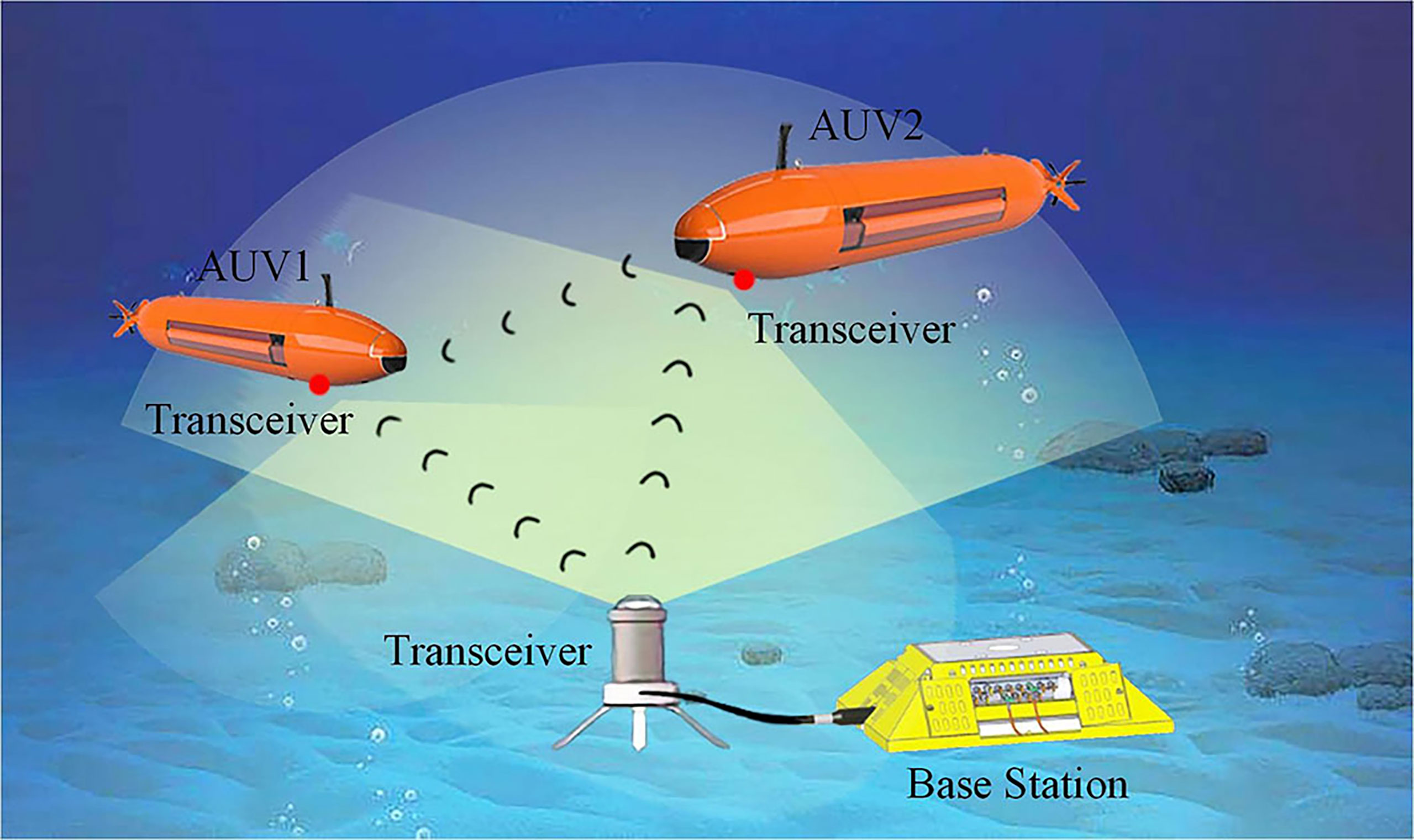
Figure 1 Schematic diagram of the seabed communication of AUV.

Since the beginning of the twenty-first century, the development of photoelectric technology and communication technology has promoted progress in underwater optical communication technology. Optical communication may use Gbps or even Tbps bandwidths (Zhang et al., 2020b). However, most underwater optical communication devices use concentrated light beams for communication. AquaOptical II is an underwater point-to-point optical communication device (Doniec and Rus, 2010). At a distance of 21 m, the two ends could conduct stable two-way communication at a rate of 5 Mbps. The disadvantage of this equipment is that it can only conduct point-to-point communication. It can only be applied to underwater information handling media that can conduct accurate position control, so its use scenarios are limited.

To achieve uniform optical coverage over the whole space, free-space optical communication (FSOC) technology was developed (Abrahamsen et al., 2021; Alexander et al., 2021; Zafar and Khalid, 2021). LED light is uniform and is not costly, so it is often used in FSOC (Huang et al., 2019; Abrahamsen et al., 2021). The Woods Hole Institute (Farr et al., 2006; Pontbriand et al., 2008; Pontbriand et al., 2016) has made outstanding research achievements in long-distance underwater optical communication. Their long-distance optical communication products use six 470 nm blue LEDs at the light-emitting end to form an evenly distributed light field. At the light-receiving end, a hemispherical photomultiplier tube (PMT) is used for optical signal acquisition. A sea trial of communication between a deep-sea seabed optical communication node and an AUV was performed for the products, and full duplex communication for distances of 0–125 m and rates of 5–20 Mbps was achieved at a depth of 2,400 m.

Some commercial products also exist, such as Sonardyne’s BlueComm modems and Aquatec’s AQUA modems. Studies regarding these products have achieved good communication results, but they rarely discuss how to design the spatial arrangements of the light-emitting devices. In fact, the structural designs of the emitters are also very important because they determine the distribution effects of the light in space. If the emitting end emits light unevenly, it can no longer conduct stable and efficient communication in space. To make the transmitter emit light evenly, a spherical transmitter with a 360° light emission range was designed (Baiden et al., 2009; Baiden and Bissiri, 2011). The light-emitting devices used were LEDs. Communication at a distance of 11 m and with a speed of 20 Mbps was achieved in a laboratory. A lake trial was completed for communication at a speed of 10 Mbps. Additionally, a new LED packaging structure was proposed (Han et al., 2019a). The light emitted by the LED with the improved structure was nearly evenly distributed in the space, a result which laid a solid foundation for optical communication in the entire space. The optical communication experiment was conducted with seven LEDs as optical transmitters. It was found that the bit error rate was very low in the range of 160°, which meets the needs of all space communication. There is still much room for improvement in FSOC light utilization and distribution uniformity, which depend on the optimization of transmitter structure. Optimizing the transmitter structure can also further improve the communication distance.

During this study, the following primary work was completed:

● A luminous model for underwater LEDs was developed and a transmitter structural design approach is proposed.

● A set of transmitter models with hemispherical coverage, high light utilization, and uniform luminescence was designed, and its luminous effect was verified.

● Through the modulation and demodulation of the photoelectric signal, a set of free-space optical communication equipment suitable for underwater use was manufactured. Experiments indicated that the communication of this system is stable and reliable.

The paper structure is described next. The approaches and corresponding simulation results are described in Sections 2–4. The experimental results are presented in Section 5. Finally, the conclusions drawn during the study are given in Section 6.

Underwater light diffusion model

The blue–green visible light band is located in the minimum attenuation window of the underwater visible light absorption spectrum. Therefore, the light in this band (wavelength between 400 and 480 nm) can be used for communication in seawater. To achieve the effect of full coverage and uniform luminescence at the transmitter, a new underwater LED blue–green light diffusion model was developed.

Underwater transmission characteristics of blue–green light

As is shown in Figure 2A, when a beam of light hits a particle underwater, three effects may occur. First, part of the light is absorbed by the particle, resulting in attenuation. Second, part of the light is scattered by the particle, which changes the transmission direction. Third, part of the light is emitted in the original direction. Through this analysis, the influences of particles on light can be approximately divided into absorption and scattering effects. These two effects weaken the light and attenuate its energy.

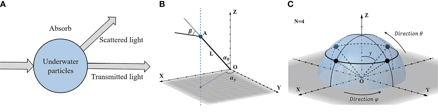
Figure 2 Physical model of (A) light colliding with an underwater particle, (B) photon emission, (C) LED spatial layout coordinate system.

If the energy of the incident light is represented by Ø₀, the light energy absorbed by the seawater is Ø_a, the light energy scattered by the seawater is Ø_b, and the transmitted light energy is Ø_t, their relationship can be expressed by Eq. (1):

To evaluate the effect of seawater on light, some parameters must be defined. a is defined as the absorption coefficient of seawater with respect to light, and it is primarily related to various particles in seawater. b is defined as the scattering coefficient of seawater with respect to light. Scattering causes irregular light transmission, leading to a pulse broadening effect and improving the bit error rate of the communication. c is defined as the extinction coefficient of seawater with respect to light.

These three coefficients are generally used to evaluate the total impact of seawater on optical transmission. The composition of seawater is complex, and the seawater quality in different sea areas is different. To facilitate the research, it is necessary to clearly define and classify different types of seawater quality.

Jerlov classified sea areas according to the spectral transmission coefficient of light per meter of sea water. Scientists then classified Jerlov’s water types in more detail (Cochenour et al., 2008). In this study, as is shown in Table 1, three types of water bodies and related parameters are cited, which provides support for the optical modeling described next.

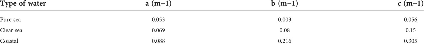
Table 1 Characteristic parameters of different types of seawater.

LED photon-free motion model

LEDs were chosen as the light source at the transmitting end for this study. The primary advantages of LED light are simple circuitry, long service life, low heat production, reliable performance, and large light-emitting range. These characteristics ensure that the light can work stably underwater for a long time, and that there are low requirements for the positioning of the receiving end.

The motion of photons generated by the LEDs was modeled based on the Monte Carlo method (Song et al., 2013). Taking the motion of a single photon as the research object, through the analysis and statistics for the motions of a large number of photons, a macroscopic light distribution result was obtained.

(1) Photon emission direction

The probabilities of photon emission in each direction are not equal. As is shown in Figure 2B, the initial photon motion direction, OA, is generated by a probability equation. The probability equation was modeled to randomly generate the initial motion conditions of the photons.

The Lambert radiation formula is a theoretical formula used to describe the relationship between the LED luminous intensity and the emission angle. According to the Lambert radiation formula, the LED radiation model can be expressed by Eq. (3):

where α represents the LED emission angle, φ(α) is the unit angle relative light intensity, and m₀ is a coefficient related to the half power angle of the LED light. Eq. (3) meets both Eqs. (4) and (5):

In Eq. (5), α_1/2 is the half power angle. The most common LED half power angles are 30° and 60°. Section 2.3 focuses on the simulation of these two types of LEDs.

To describe the random emission directions of the photons, an equal probability random number, ϵ∈[0, 1] , was constructed:

Eq. (7) was obtained by combining Eqs. (4) and (6):

By constructing the random number, the required random emission angle can be generated. α₀ represents the angle between the exit direction and the z-axis, and α₀∈[0, π/2] . To obtain the initial photon emission direction, the included angle with the y-axis is also required. Similarly, the angle with the y-axis (α_y) is also a random value, and α_y has equal probability in [−π, π]. Another random number, , was also constructed.

α_y∈[−π, π] . If the photon emission velocity is U₀, the initial photon emission direction is expressed by Eq. (9):

(2) Free motion distance and energy

The free motion distance of the photons refers to the distance the photons travel before colliding with particles, and it is calculated using Eq. (10):

In Eq. (10), τ represents a random number evenly distributed between 0 and 1, and c is the extinction coefficient of seawater with respect to light, which was introduced in Section 2.1. After scattering or absorption, the photon energy decays:

where e_out and e_in represent the energy before and after particle collisions, respectively, and a is the light absorption coefficient.

(3) Scattering

As shown in Figure 2B, light scattered in water changes the direction of photon motion and forms a scattering angle (β). The H–G phase function was used in this study for the scattering analysis, and its expression is given in Eq. (12):

In Eq. (12), g =< cosβ >, which is not only the scattering asymmetry factor, but also the average value of the cosine of the scattering angle. When g = −1, all the light is backscattered. g = 0 indicates isotropic light scattering. When g = 1, all the light is forward-scattered. According to Eq. (12), the random function for the scattering angle is given by Eq. (13):

where μ is a random number evenly distributed between 0 and 1. σ represents the scattering pitch angle, which is a random value:

If (U_x, U_y, U_z) is the photon motion vector before the last collision and (U_x1, U_y1, U_z1) is the photon motion vector after that, when U_z ≥ 0.999, Eq. (15) applies:

Otherwise, Eq. (16) is used for calculations:

The equations presented above comprise the underwater light diffusion model developed during this study.

LED luminous simulation

To test this model, the luminescence of two common LEDs was simulated: LEDs with a half power angle of 30° and LEDs with a half power angle of 60°. The asymmetry coefficient, g, was taken as 0.924, and the results are shown in Figure 3.

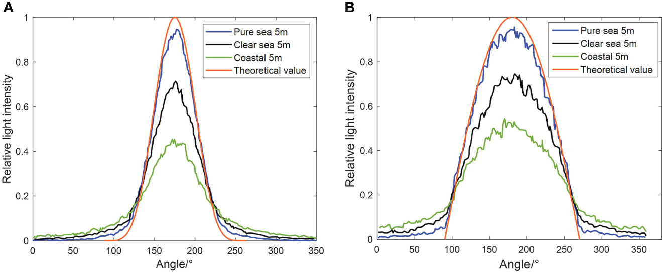
Figure 3 Luminous effects of single LEDs with half power angles of (A) 30° and (B) 60°.

In pure sea water, the theoretical results of the two LEDs are approximately consistent with the actual results, but there are also some differences. The reason for the differences is that the absorption of light by the water makes the intensity in the transmission direction (an angle of 180°) lower than the theoretical value. Light scattering also makes the light intensity extend to both sides. Comparing the transmission results of single LEDs in different water qualities indicates that a worse water quality leads to a greater difference between the actual and theoretical light intensity distributions and more obvious absorption and scattering effects. Overall, the simulation results for the single LEDs are consistent with the theoretical predictions.

LED array layout

The placement of the LEDs in the space was designed to achieve the effect of uniform light coverage in the space. Figure 2C shows the coordinate system of the light-emitting end. It is assumed that the LEDs are distributed on a sphere with radius r, and that the luminous direction is consistent with the normal direction. N LEDs emit K photons in total, and some photons reach the sphere at a distance L from the center. The spatial luminous effect of each LED can be described by two directions, φ and θ, in spherical coordinates. The influences of the two factors on the light intensity distribution do not interfere with each other, so they were studied separately.

φ direction

First, the change in light intensity caused by the arrangement of LEDs in the φ direction was studied. For the convenience of design, N was set as a number that can be divided by 360, that is, N = 1, 2, 3, 4, 5, 6, 8, 9, 10, 12, 15, …. If V₁ is the emitting direction of the LED numbered 1 and V_i is the emitting direction of the LED numbered i, then i∈[1, N] and Eq. (17) applies:

In Eq. (17), R_i1 represents the rotation matrix around the z-axis:

The distribution of photons in the φ direction reaching the sphere is measured. There are two indicators to evaluate the effect of spatially distributed light: the minimum photon number in space and the luminous uniformity.

(1) Minimum photon number

The range of φ is [0°, 360°] and is divided into 360 intervals, where each interval is 1°. The total number, m_i, of photons reaching this interval is calculated and its minimum value is found. This minimum value is defined as M_i:

M_i can show the influence of the number of LEDs on the minimum photon number when the LEDs are evenly arranged.

(2) Luminous uniformity

The standard deviation of the number of photons reaching these intervals is defined as the luminous uniformity, ρ_i:

In Eq. (21), $\overline{m}$ represents the average value of the photons and n = 360.

To obtain the best design scheme for the transmitter LED array, the luminescence of the LED array in the φ direction was analyzed using the mathematical model described above. When the total number of photons is the same, different numbers of LED groups are evenly distributed along the circumference in the φ direction. The photon distributions in space are compared. As shown in Figure 4, with increases in the number of LED groups, the light intensity fluctuations become smaller and the luminous uniformity improves.

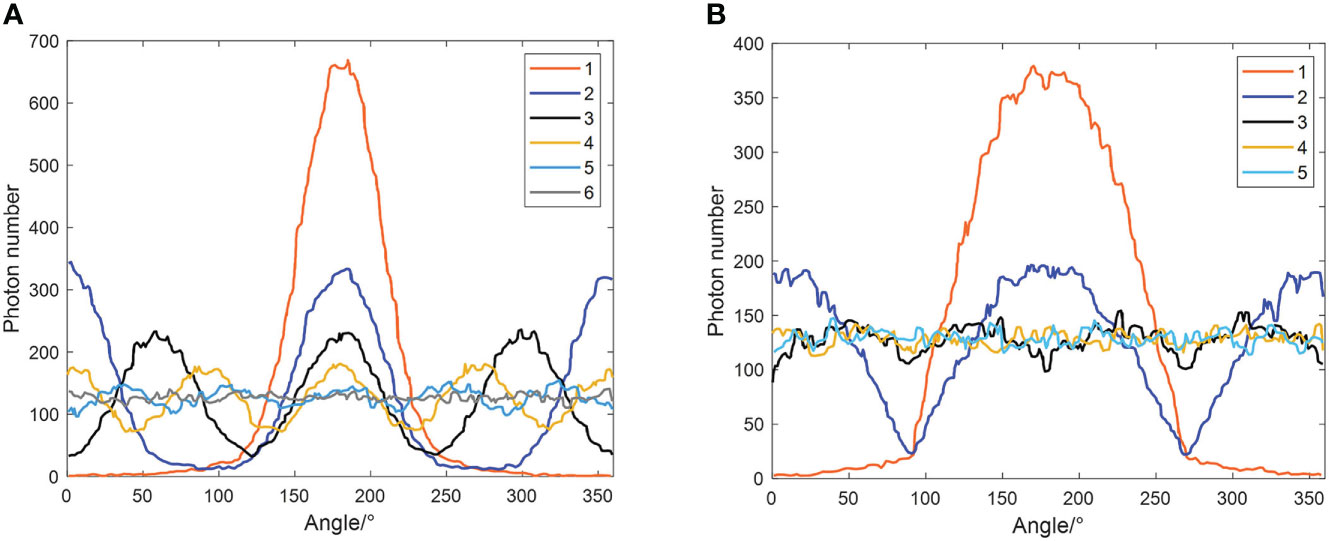
Figure 4 Photon distributions in the φ direction of the LED array with half power angles of (A) 30° and (B) 60°.

Then, the minimum photon number and the standard deviation along the circumferential direction are used to compare the luminous uniformity, as shown in Figure 5. For different water qualities, when the half power angle is 30° and six or more groups of LEDs are distributed along the circumference, the minimum photon number and the standard deviation remain nearly unchanged, indicating that the light distribution is uniform.

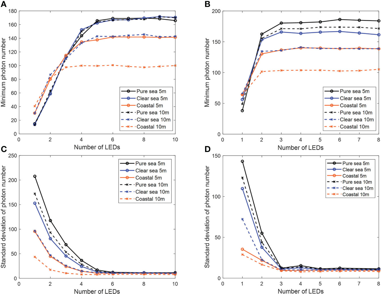
Figure 5 Minimum number of photons in the φ direction for LED arrays with half power angles of (A) 30° and (B) 60°. Standard deviation of the photon number in the φ direction for LED arrays with half power angles of (C) 30° and (D) 60°.

Similarly, when the half power angle is 60° and three or more groups of LEDs are distributed along the circumference, the light distribution is uniform. Comparing the luminous effects of the two LEDs indicates that the LEDs with a half power angle of 60° achieve a more uniform luminous effect with a smaller quantity of LEDs. Therefore, four groups of LEDs with a half power angle of 60° were used for the next analysis.

θ direction

The analysis methods for the θ and φ directions are the same. Since the AUV will have depth control when sinking, it will not be at a large angle with the base station. Therefore, it is sufficient for the LED to cover an angle of 160° in the θ direction. The included angle between the LED and the z-axis is represented by γ. Since the photons in the area below the hemisphere are useless, the light effective utilization, ω, was used to quantify the useful light.

In Eq. (23), n₀ represents the number of photons emitted and n₁ is the number of photons in the upper hemisphere. When the number of LEDs is odd, to ensure light symmetry, the direction of one LED is vertically upward. When the number of LEDs is even, the LEDs are symmetrically distributed around the z-axis.

The luminescence in the θ direction was then simulated and analyzed. As shown in Figure 6, when γ∈ (60°, 65°) , the photon standard deviation is small and the minimum photon density is large. A smaller included angle leads to a greater effective light utilization rate. Considering these three factors comprehensively, γ = 60° was taken as the design criterion.

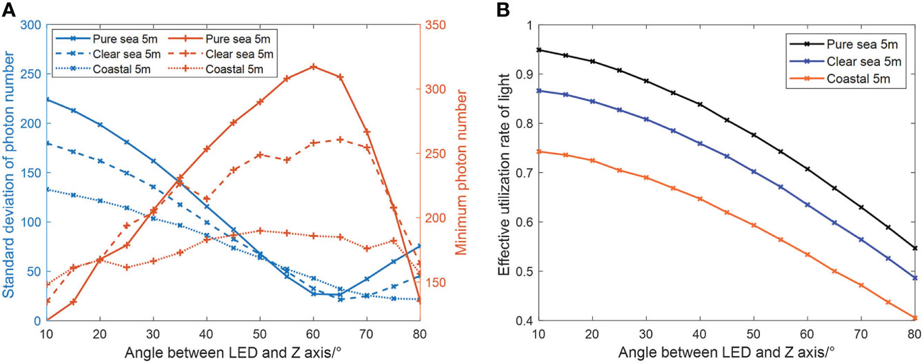
Figure 6 (A) Minimum photon number and standard deviation, (B) effective utilization of light in the θ direction of the LED array with a half power angle of 60°.

Transmitter luminous simulation

Combined with the analyses in the φ and θ directions, the structural design of the transmitter was completed. The design consists of four groups of LEDs with a half power angle of 60° that are evenly distributed along the φ direction, with an included angle between these LEDs and the z-axis of 60°.

The transmitter model was imported into the optical simulation software Trace Pro for testing. As shown in Figure 7, the light is evenly distributed in the φ directions, and the coverage angle of the light in the θ direction increased to 83°. This model ensures uniform light distribution over a large range, which shows that the design is reasonable.

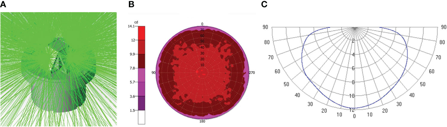
Figure 7 Luminous effect of (A) the transmitter and (B) the transmitter in the φ direction and (C) in the θ direction.

Photoelectric signal processing

Avalanche diodes can detect weak light with a high response frequency. An avalanche diode was chosen as the receiving device when designing the system. To achieve stable communication, photoelectric signal processing is needed at the receiving end.

Noise filtering

The photocurrent of an avalanche diode must be amplified and shaped by an operational amplifier circuit. This process requires a high bias voltage and generates a large amount of noise, so it must be denoised before output.

Blue light band communication with a wavelength of approximately 400–480 nm was used. According to this characteristic, the blue light filter can be used to filter out most of the light with wavelengths not in this band. In this work, two different types of interference must also be eliminated: various noise interferences generated in the circuit and ambient light interference. In this work, a second-order Butterworth low-pass filter was used to filter the circuit noise. This filter has a good suppression effect on high-frequency signals and can be used to filter out high-frequency noise. A finite length unit impulse response digital filter (FIR) was used to filter the ambient light interference. The FIR filter ensures arbitrary amplitude frequency characteristics and strict linear phase frequency characteristics simultaneously, which can effectively filter out low-frequency sinusoidal ambient noise.

Improved 16-PPM algorithm

To avoid the interference of the environment and reduce the bit error rate, it is necessary to modulate and demodulate the optical signal. Pulse modulation is generally used for long-distance underwater optical communication, that is, optical pulses are used to transmit optical information. The pulse position modulation (PPM) method has the lowest bit error rate for long-distance underwater optical communication. Considering the transmission efficiency, the 16-PPM method was finally selected for information transmission.

The traditional PPM method has some defects. Owing to the limited production process and the influence of temperature, there are irregular errors in the clock frequency of the hardware system at the transmitter and receiver. This problem leads to continuous changes in the clock phase between the receiver and the transmitter, resulting in some misjudgments. For example, when the rising edge of a pulse reaches the receiving end, the clock at the receiving end is in the low state and the information cannot be effectively collected. Instead, it must wait until the high state of the next clock, so the arrival time is misjudged.

The solution to this problem is described next. The time between receiving the rising edge of one pulse and receiving the rising edge of the next pulse is measured. This time interval is used to accurately judge the distance between two adjacent pulses, so as to ensure the accuracy of demodulation. As is shown in Figure 8, two additional measures are also taken to increase the stability of communication.

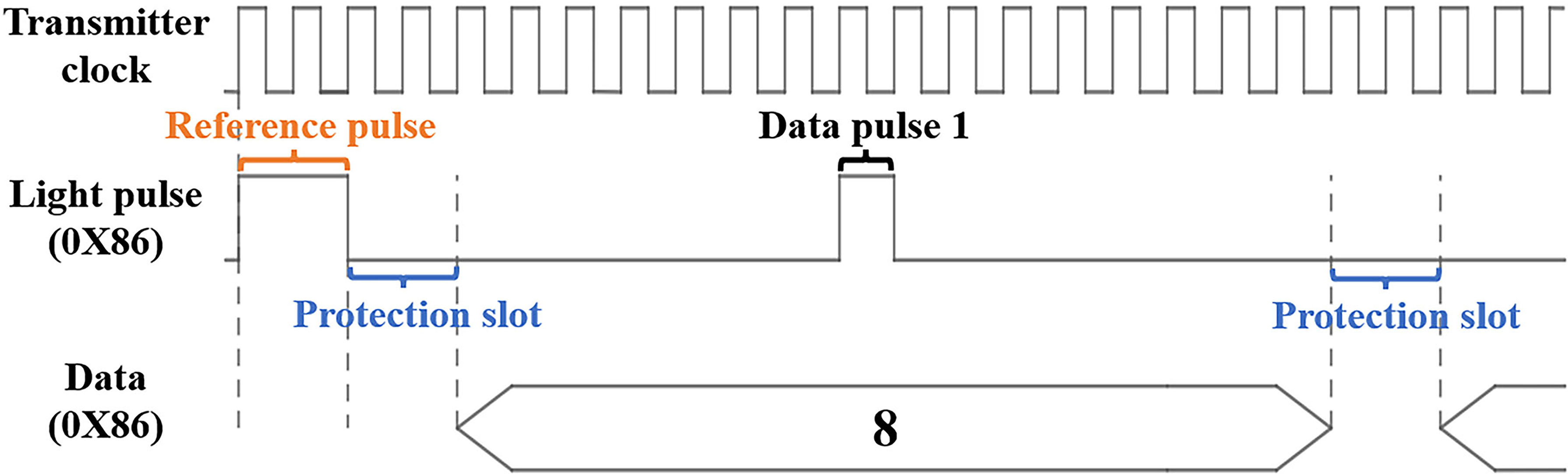
Figure 8 Schematic diagram of the improved 16-PPM method.

(1) Increase the initial reference pulse

The length of the reference pulse is set to twice that of an ordinary pulse to indicate the beginning of communication. This is done to avoid misjudging the reference pulse due to short-term interference and to achieve frame synchronization.

(2) Add a protection slot

A blank time slot is placed after each pulse to prevent the front and rear pulses from interfering with each other. Although this change takes up time, it improves the communication stability.

Experimental results

Prototype

A system prototype was manufactured according to the method described above. The prototype was divided into two primary parts, a transmitter and a receiver, as shown in Figure 9. The transmitter used LEDs with a half power angle of 60° as the light-emitting device. Four groups of LEDs were evenly distributed along the circumference with an inclination of 60°. Avalanche diodes were used as signal receiving devices. An FPGA processing board was used for photoelectric signal modulation and demodulation, information caching, and processing. The devices were located in a mechanical pressure housing with a glass observation window that was sealed with an O-ring and a rubber gasket. We test the application reliability of the prototype through a heat dissipation simulation and pressure response experiment.

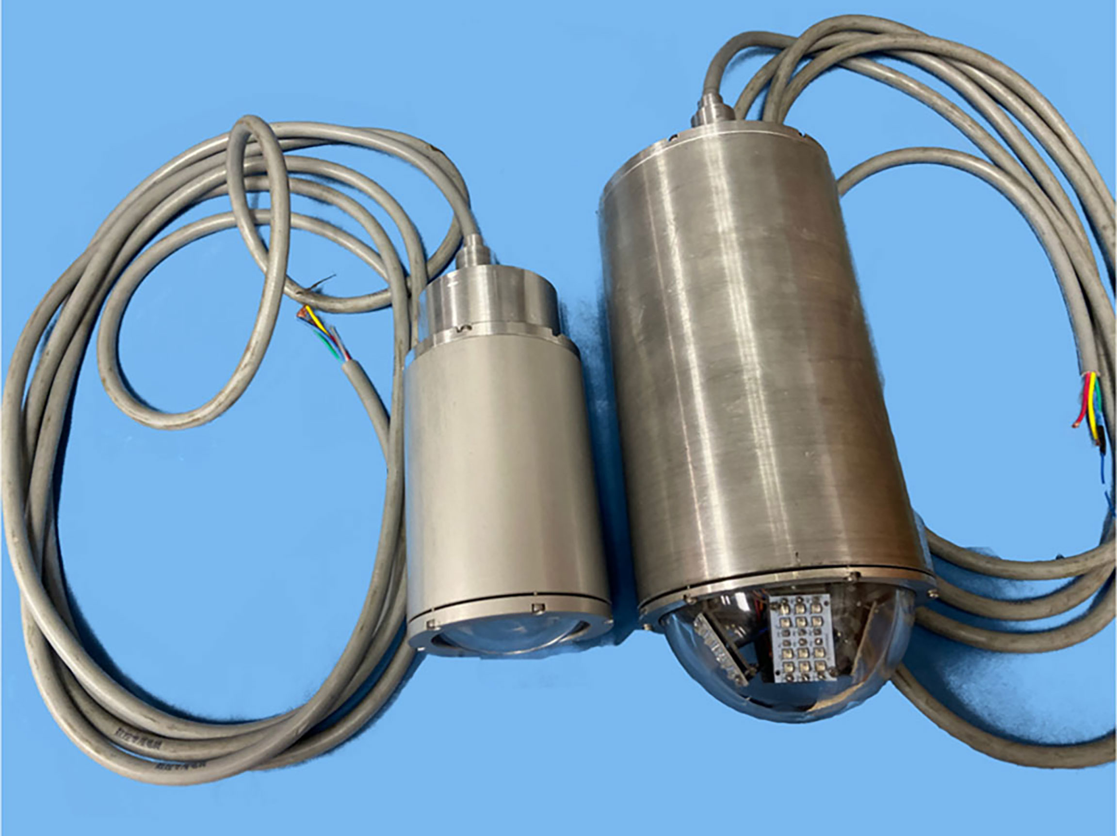
Figure 9 Prototype: receiver on the left and transmitter on the right.

When an LED is emitting light, only 20%–30% of the energy is converted into light energy, and the rest is converted into heat energy. If the heat energy cannot be dispersed well, the temperature of the LED will rise rapidly. This will lead to a rapid decline in the luminous efficiency and will ultimately affect the communication effect. The maximum power of the system is 14 W; we simulate the heat dissipation of the transmitter, and the results are shown in Figure 10. When the system is turned on at full power, high temperatures are concentrated at the luminous LED (approximately 35°C). At this temperature, the LED operation will not be significantly affected. This proves that the design presented in this paper is feasible.

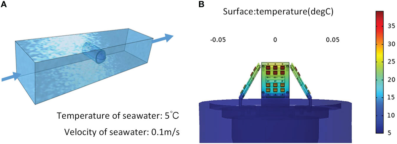
Figure 10 Heat dissipation simulation: (A) simulation model, (B) heat dissipation diagram of the transmitter when the thermal power is 14 W.

To test the reliability of the equipment for deep-sea applications, we use the software ANSYS to conduct a withstand pressure analysis of the pressure housing. Because the housing is centrosymmetric, the simulation model can be simplified to a two-dimensional model as shown in Figure 11A. The housing is made of 6061-T6 aluminum alloy with a yield strength of 275 MPa. We add 30-MPa pressure to the outer surface of the housing in all directions, and the results are shown in Figure 11B. The simulation shows that there are stress concentration points at some corners that exceed the yield strength, so we add chamfers at the corners. As shown in Figure 11C, D, the pressure test is carried out on the prototype using a high-pressure experimental chamber. Since the target application depth of the prototype is 1500 m, the test pressure is set to 15 MPa. The prototype can withstand high pressure without water leakage and can be used in the deep sea normally.

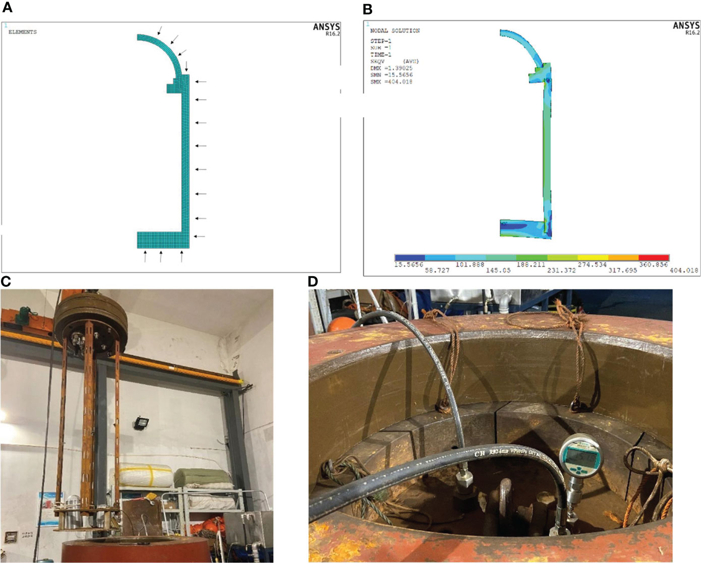
Figure 11 The pressure withstand experiment: (A) load model, (B) stress diagram of housing, (C) test in high-pressure experimental chamber, (D) pressure value.

Basic function test

As shown in Figure 12A, C, the basic function of the system was tested in the air. First, the light intensity of the transmitter was tested in all directions. A comparison between Figure 12B and Figure 7C shows that the measured light intensity curve was approximately the same as that from the simulation results. The difference is that the actual curve lies closer to the central axis than the curve from the simulation results. It was speculated that the reason for the difference is that the observation window outside the LED impacted the light distribution, causing the light to converge more toward the central axis. Then, the performance of the receiver was tested when receiving optical pulses of different frequencies. As shown in Figure 12D, the receiver successfully received optical pulses of different frequencies. Although the square wave signal was slightly distorted, the communication quality was not affected.

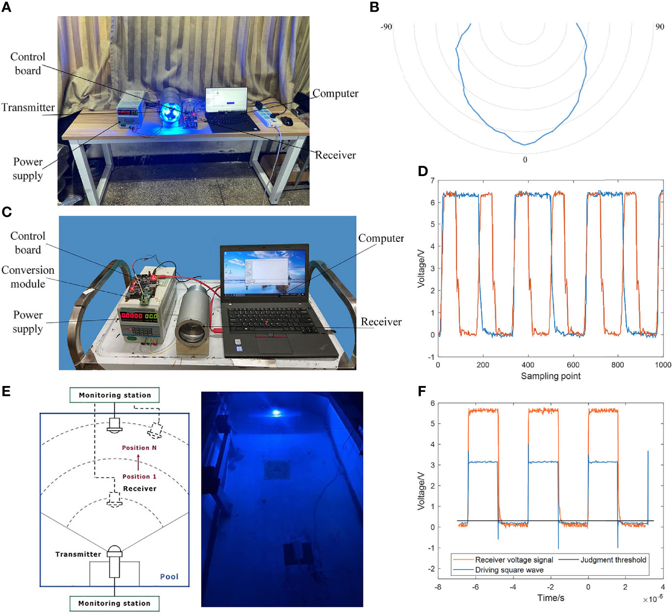
Figure 12 (A) Transmitter test system. (B) Actual luminous effect of the transmitter. (C) Receiver test system. (D) Receiving effect of the receiver on 2.5-MHz and 5-MHz optical pulses. (E) Underwater experiment. (F) Diagram comparing the received optical pulse signal and the driving signal.

Underwater communication experiment

Experiments on the underwater communication effect of the optical communication system were conducted, as shown in Figure 12E. The reception of square wave signals in the optical communication system was tested. On this basis, the bit error rate of the communication between the transmitter and the receiver at different distances was measured.

First, a 3.5 m short-range communication experiment was performed. During the test, the instantaneous power of the transmitter was 10 W and the square wave frequency was 2.5 MHz. The shape of the received pulse is shown in Figure 12F. The received pulse was a relatively regular square wave. Owing to the small distance, it differed slightly from the waveform in the air, only the falling edge was relatively slow and had a certain lag phenomenon. The rising edges of the driven and received signals coincided, while the shapes of the falling edges were different. Therefore, it is feasible to use the rising edge as a benchmark.

The bit error rates for three different communication rates are shown in Table 2. The bit error rate of a certain communication distance is the maximum value of the bit error rate of three randomly sampled points when γ∈[−30°, 30°] . The data in this table demonstrate that the short-distance communication quality of the new equipment is very good.

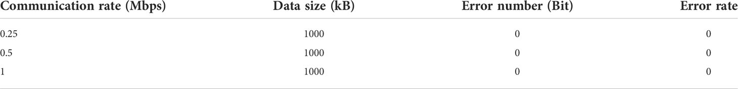
Table 2 Statistical table of communication bit error rates at a distance of 3.5 m.

Then, a long-distance communication experiment was conducted. The bit error rates for the long-distance communication are shown in Table 3 (NVI = no valid information). When the distance is greater than 12 m, the bit error rate begins to rise rapidly from 0. Demodulation cannot be performed at 15 m, a situation which applies to all three rates. Therefore, when the transmitter power is 10 W, the maximum underwater communication distance is 12–13 m. For larger distances, the bit error rate rises rapidly, and communication cannot continue.

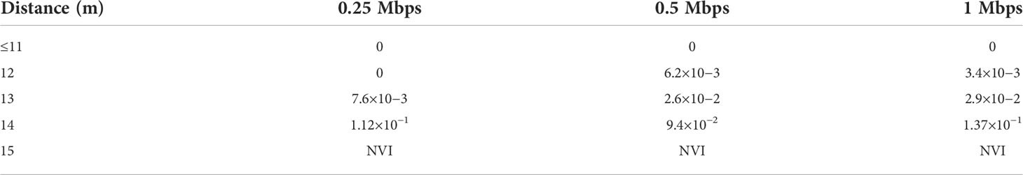
Table 3 Bit error rates for different distances and communication rates.

To explain this phenomenon, the optical pulse signal at a distance of 13 m was measured. Figure 13 shows that the received optical pulse is seriously deformed. Although the photovoltage was still above 0.5 V at the beginning, the voltage becomes increasingly smaller after that. When the distance continues to rise, it is predicted that part of the optical pulse voltage will be lower than the critical voltage, so that the pulse time for judgment will be shorter. This situation does not meet the conditions of demodulation, and the bit error rate will increase rapidly.

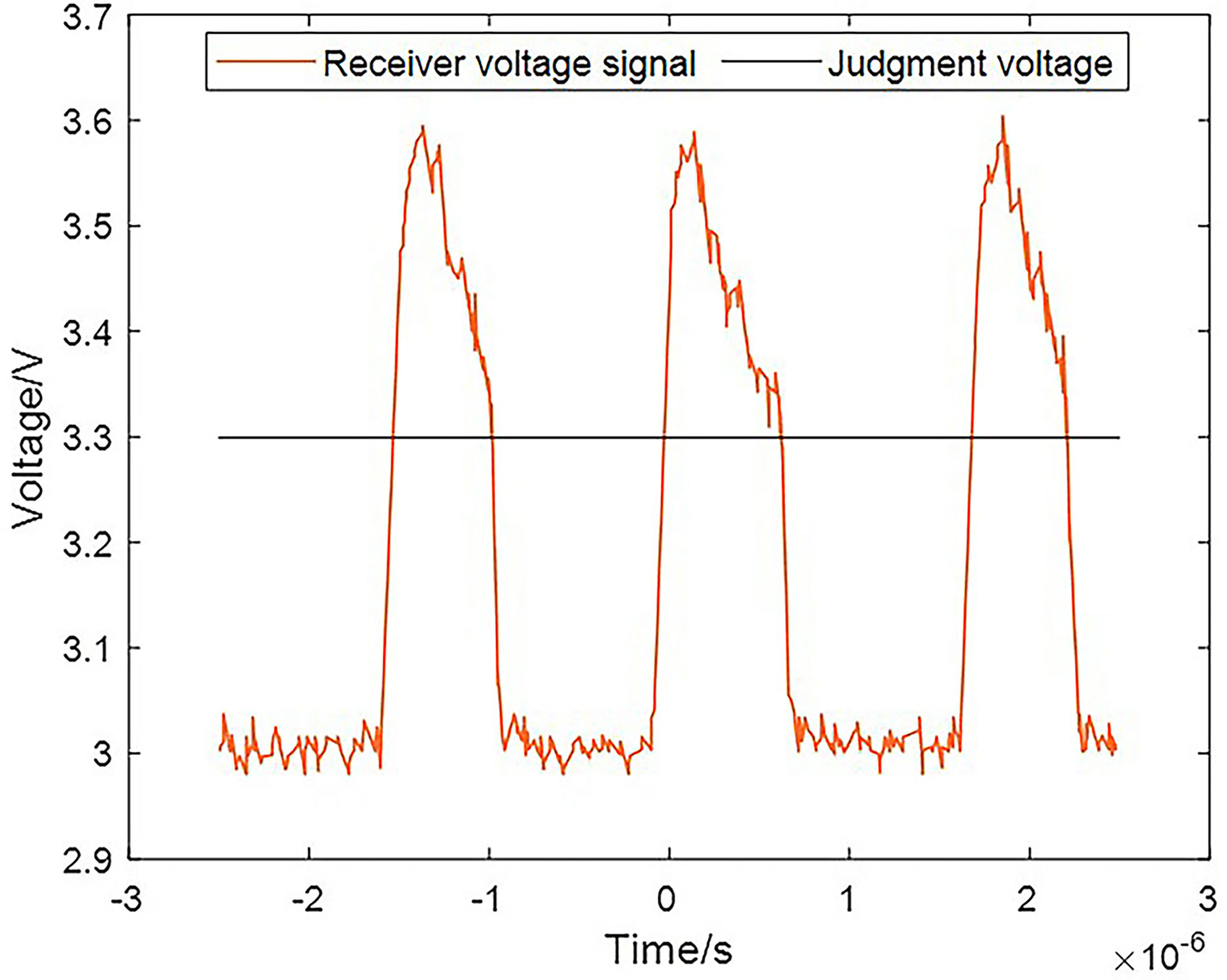
Figure 13 Optical pulse signal at a distance of 13 m.

The experiments described above indicate that this new system achieved the expected goal better. When the transmitter power is 10 W, the maximum communication distance is 12–13 m. Theoretically, when the power of the transmitting end is 20 W, the communication distance will increase to approximately $\sqrt{2}x$, that is, the communication distance will be 17–18.5 m. This is not the distance limit. The communication distance can be further improved by reducing the judgment threshold.

Conclusions

In this study, based on the research background of the information communication modes between a seabed observation base station and an information transmission medium, a space optical communication method suitable for the deep sea was proposed. Through research regarding the underwater luminescence mechanism of light-emitting elements, a transmitter was designed. By analyzing the transmission characteristics of underwater optical pulses and exploring photoelectric noise filtering methods, a receiver was designed. Existing pulse modulation and demodulation methods were improved to achieve better results. Finally, a complete set of space free optical communication prototypes was developed that can be used underwater. The simulations and basic function tests show that the prototype has good heat dissipation and high-pressure resistance, and the prototype can be used in the deep sea. The communication experiments demonstrate that our system has good communication performance. The reliability and applicability of the system verify that our method is feasible and practical.

Data availability statement

The original contributions presented in the study are included in the article/supplementary material. Further inquiries can be directed to the corresponding author.

Author contributions

YC: Methodology, Project administration, Investigation. LZ: Writing - Original Draft, Visualization, Validation. YL: Data Curation, Software. All authors contributed to the article and approved the submitted version.

Funding

This work was supported by National Natural Science Foundation of China (No.51979246), the National Key Research and Development Program of China (No. 2021YFC2800202), the Strategic Priority Research Program of Chinese Academy of Sciences No. XDA22010402) and Ningbo Science and Technology Innovation 2025 Major Special Project (2021Z079).

Conflict of interest

The authors declare that the research was conducted in the absence of any commercial or financial relationships that could be construed as a potential conflict of interest.

Publisher’s note

All claims expressed in this article are solely those of the authors and do not necessarily represent those of their affiliated organizations, or those of the publisher, the editors and the reviewers. Any product that may be evaluated in this article, or claim that may be made by its manufacturer, is not guaranteed or endorsed by the publisher.

References

Abrahamsen F. E., Ai Y., Wold K., Mohamed M. (2021). Free-space optical communication: From space to ground and ocean. IEEE Potentials. 40, 18–23. doi: 10.1109/MPOT.2020.2979057
Alexander B., Felix S., Igor M. (2021). “Practical applications of free-space optical underwater communication,” in 2021 Fifth Underwater Communications and Networking Conference (UComms)., Vol. 2021. (Lerici, Italy: IEEE), 2–6.
Baiden G., Bissiri Y. (2011). “High bandwidth spherical optical wireless communication for subsea telerobotic mining,” in OCEANS'11 MTS/IEEE KONA. (Waikoloa, HI, US: IEEE), 1–4. doi: 10.23919/oceans.2011.6106950
Baiden G., Bissiri Y., Masoti A. (2009). Paving the way for a future underwater omni-directional wireless optical communication systems. Ocean Eng. 36, 633–640. doi: 10.1016/j.oceaneng.2009.03.007
Cao X.-L., Jiang W., Tong F. (2018). Time reversal MFSK acoustic communication in underwater channel with large multipath spread. Ocean Eng. 152, 203–209. doi: 10.1016/j.oceaneng.2018.01.035
Che X., Wells I., Dickers G., Kear P., Gong X. (2010). Re-evaluation of RF electromagnetic communication in underwater sensor networks. IEEE Commun. Mag. 48, 143–151. doi: 10.1109/MCOM.2010.5673085
Cochenour B. M., Mullen L. J., Laux A. E. (2008). Characterization of the beam-spread function for underwater wireless optical communications links. IEEE J. Ocean. Eng. 33, 513–521. doi: 10.1109/JOE.2008.2005341
Doniec M., Rus D. (2010). “BiDirectional optical communication with AquaOptical II,” in 12th IEEE Int. Conf. Commun. Syst. 2010, ICCS, Vol. 2010. 2010 IEEE International Conference on Communication Systems. (Singapore: IEEE) 390–394. doi: 10.1109/ICCS.2010.5686513
Farr N., Chave A. D., Freitag L., Preisig J., White S. N., Yoerger D., et al. (2006). Optical modem technology for seafloor observatories. Ocean 2006, 1–7. doi: 10.1109/OCEANS.2006.306806
Han X., Yin J., Tian Y., Sheng X. (2019b). Underwater acoustic communication to an unmanned underwater vehicle with a compact vector sensor array. Ocean Eng. 184, 85–90. doi: 10.1016/j.oceaneng.2019.03.024
Han B., Zhao W., Zheng Y., Meng J., Wang T., Han Y., et al. (2019a). Experimental demonstration of quasi-omni-directional transmitter for underwater wireless optical communication based on blue LED array and freeform lens. Opt. Commun. 434, 184–190. doi: 10.1016/j.optcom.2018.10.037
Huang X., Yang F., Song J. (2019). Hybrid LD and LED-based underwater optical communication: State-of-the-art, opportunities, challenges, and trends [Invited]. Chin. Opt. Lett. 17, 100002. doi: 10.3788/col201917.100002
Liu L., Liao Z., Chen C., Chen J., Niu J., Jia Y., et al. (2019). A seabed real-time sensing system for in-situ long-term multi-parameter observation applications. Sensors. (Switzerland). 19. doi: 10.3390/s19051255
N’Doye I., Zhang D., Alouini M. S., Laleg-Kirati T. M. (2021). Establishing and maintaining a reliable optical wireless communication in underwater environment. IEEE Access 9, 62519–62531. doi: 10.1109/ACCESS.2021.3073461
Pontbriand C., Farr N., Hansen J., Kinsey J. C., Pelletier L. P., Ware J., et al. (2016). “Wireless data harvesting using the AUV sentry and WHOI optical modem,” in Ocean. OCEANS 2015 - MTS/IEEE Washington. (Washington, DC, USA: IEEE). doi: 10.23919/oceans.2015.7401985
Pontbriand C., Farr N., Ware J., Preisig J., Popenoe H. (2008). Diffuse high-bandwidth optical communications. (Quebec City, QC, Canada: IEEE).
Sahoo A., Dwivedy S. K., Robi P. S. (2019). Advancements in the field of autonomous underwater vehicle. Ocean Eng. 181, 145–160. doi: 10.1016/j.oceaneng.2019.04.011
Sherlock M., Marouchos A., Williams A. (2014). “An instrumented corer platform for seabed sampling and water column characterisation,” in Ocean. OCEANS 2014 - TAIPEI. (Taipei, Taiwan: IEEE). doi: 10.1109/OCEANS-TAIPEI.2014.6964367
Song S., Kobayashi Y., Fujie M. G. (2013). Monte-Carlo simulation of light propagation considering characteristic of near-infrared LED and evaluation on tissue phantom. Proc. CIRP. 5, 25–30. doi: 10.1016/j.procir.2013.01.005
Su R., Zhang D., Li C., Gong Z., Venkatesan R., Jiang F. (2019). Localization and data collection in AUV-aided underwater sensor networks: Challenges and opportunities. IEEE Netw. 33, 86–93. doi: 10.1109/MNET.2019.1800425
Yoon S., Azad A. K., Oh H., Kim S. (2012). AURP: An AUV-aided underwater routing protocol for underwater acoustic sensor networks. Sensors 12, 1827–1845. doi: 10.3390/s120201827
Zafar S., Khalid H. (2021). Free space optical networks: Applications, challenges and research directions. Wirel. Pers. Commun. 121, 429–457. doi: 10.1007/s11277-021-08644-4
Zhang D., N’doye I., Ballal T., Al-Naffouri T. Y., Alouini M. S., Laleg-Kirati T. M. (2020a). Localization and tracking control using hybrid acoustic-optical communication for autonomous underwater vehicles. IEEE Internet Things. J. 7, 10048–10060. doi: 10.1109/JIOT.2020.2995799
Zhang S., Yang X., Wang Y., Zhao Z., Liu J., Liu Y., et al. (2020b). Automatic fish population counting by machine vision and a hybrid deep neural network model. Animals 10, 1–17. doi: 10.3390/ani10020364
Keywords: seabed observation platform, free-space optical communication, underwater wireless communication, space luminescence array, pulse modulation and demodulation
Citation: Chen Y, Zhang L and Ling Y (2022) New approach for designing an underwater free-space optical communication system. Front. Mar. Sci. 9:971559. doi: 10.3389/fmars.2022.971559
Received: 17 June 2022; Accepted: 22 July 2022;
Published: 11 August 2022.
Edited by:
Shaowei Zhang, Institute of Deep-Sea Science and Engineering (CAS), ChinaReviewed by:
Shengxi Diao, East China Normal University, ChinaWenyu Cai, Hangzhou Dianzi University, China
Yanbo Wu, Institute of Acoustics (CAS), China
Copyright © 2022 Chen, Zhang and Ling. This is an open-access article distributed under the terms of the Creative Commons Attribution License (CC BY). The use, distribution or reproduction in other forums is permitted, provided the original author(s) and the copyright owner(s) are credited and that the original publication in this journal is cited, in accordance with accepted academic practice. No use, distribution or reproduction is permitted which does not comply with these terms.
*Correspondence: Yanhu Chen, yanhuchen@zju.edu.cn