Dispersion of subsurface lagrangian drifters in the northeastern Gulf of Mexico

1 Introduction

Transport pathways in the Gulf of Mexico (GoM) are controlled by large-scale circulation associated with the unstable Loop Current, eddies, bathymetric effects, wind forcing, and boundary-trapped waves. The dominant current in the GoM is the Loop Current, formed from the intrusion of warm Caribbean water into the Gulf across the sill between the Yucatan peninsula and Cuba. From this Loop Current, large eddies are produced, which may detach and dominate the circulation over most of the interior of the Gulf. Frontal instability of the Loop Current is thought to be partly responsible for a complex field of eddies in the northern GoM (Huh et al., 1981; Vukovich and Maul, 1985; Maslo et al., 2020). Most of the time, the Loop Current is south of about 26.5°N (Dukhovskoy et al., 2015). Thus, the Loop Current itself does not impinge on the northern slope region but generates a cascade of smaller-scale motions that subsequently intrude upon the northern Gulf slope and are partly responsible for the eddy activity there (Hamilton et al., 2000; Ohlmann et al., 2001; Ohlmann and Niiler, 2005; Hamilton and Lee, 2005; Hamilton, 2007). In addition, flow along the northern Gulf slope can be forced remotely by Loop Current interaction with the slope further south and east along the Florida escarpment (Oey and Lee, 2002; Hamilton and Lee, 2005; Nguyen et al., 2015; Jouanno et al., 2016; Liu et al., 2018).

In the northeast GoM, wind-driven currents dominate transport on the wide and shallow continental shelf but become only one of several factors controlling transport farther offshore (Weisberg et al., 2005), where mesoscale eddies with scales of 10–100 km are of equal or greater importance (Hamilton and Lee, 2005). Even smaller, submesoscale flow structures are gaining recognition as important components of both upper and deep ocean dispersion (Zhong and Bracco, 2013; Poje et al., 2014; Bracco et al., 2016; Liu et al., 2018).

Cyclonic (anticlockwise) and anticyclonic (clockwise) eddies have frequently been observed in DeSoto Canyon (DSC), located in the northeastern GoM (Hamilton et al., 2000; Wang et al., 2003; Hamilton, 2007; Hamilton et al., 2015). These eddies, along with wind forcing, have been associated with lower frequency ocean currents energetic at periods of weeks to months (Wang et al., 2003; Hamilton and Lee, 2005; Teague et al., 2006; Carnes et al., 2007; Hallock et al., 2009). Though most of the eddies are formed remotely and intrude upon the northeastern GoM, it has been proposed that some eddies might be locally generated in DSC (Weisberg et al., 2005), due to strong along-slope flow interacting with sharp bends in the bathymetry. In addition to eddy activity, coastally trapped shelf waves have been inferred from mooring data west of DSC (Carnes et al., 2007; Hallock et al., 2009). Potential driving forces are winds along the West Florida Shelf (Carnes et al, 2007) and eddies impacting DSC along the Mississippi–Alabama slope (Hallock et al., 2009).

Numerous observational studies (Hamilton et al., 2000; Wang et al., 2003; Leben, 2005; Liu and Weisberg, 2005; Ohlmann and Niiler, 2005; Hamilton, 2007; Hamilton et al., 2011; Liu et al., 2016; Furey et al., 2018; Perez-Brunius et al., 2018, to name a few) and numerical simulations (Morey et al., 2005; Nguyen et al., 2015; Bracco et al., 2016) have shown that the flow in the northeastern GoM is complex. This flow is often characterized by high temporal and spatial variability, which allows variable shear flows, as well as high and low vorticity environments, to exist on a range of scales. Eddies in such an environment will experience varying trap zone sizes (Shapiro et al., 1997), leading to the capture and/or release of particles as the eddies propagate through this fluctuating background flow. In this manner, eddies can transport particles away from preferred flow pathways, which are often constrained by ocean bathymetry at depth (Weisberg et al., 2011), and into the interior of the basin.

We postulate that the capture-and-release effect of eddies in a variable background flow affects particle dispersion by transporting particles away from depth-constrained along-slope pathways. This allows particles to spread more uniformly throughout the northeastern GoM and increases their residence time within the eastern GoM. To explore this hypothesis, we will use subsurface RAFOS drifter data from the eastern GoM, as well as output from a 5-year Regional Ocean Modeling System (ROMS) simulation over the entire GoM.

The paper is organized as follows. RAFOS drifter data and an overview of the ROMS model simulation are described in Materials and methods. respectively. A brief outline of self-organizing maps (SOM) is located at the end of Materials and methods, followed by results and a discussion.

2 Materials and methods

Lagrangian surface and subsurface drifter track data are usually employed in a statistical fashion to observe ocean currents and estimate turbulence and diffusivity within specific flow regions (LaCasce, 2008; Salle et al., 2008; Balwada et al., 2016; Balwada et al., 2021). In this paper, we consider the tracks of five subsurface RAFOS drifters, deployed in DSC over approximately 60 days (15 June 2012–05 August 2012). These drifters were part of the Deep-C Dispersion Experiment in the Eastern Gulf of Mexico to investigate the dispersion in DSC and the northeastern GoM (Hancock and Speer, 2013). To expand upon the results from this novel RAFOS drifter experiment, we use the output from a 5-year free-running version of the ROMS data assimilative counterpart over the entire GoM (Maslo et al., 2020).

2.1 RAFOS float data

Thirty-six autonomous drifters, called RAFOS drifters, were deployed at 11 locations in DSC in May of 2012 (Figure 1), as part of the Deep-C Dispersion Experiment in the Eastern Gulf of Mexico (Hancock and Speer, 2013). The RAFOS float is an acoustically tracked subsurface drifter (Rossby et al., 1986) programmed to listen for coded acoustic signals from distant moored sound sources. Using the measured arrival times of the sound signal and the speed of sound in water, the positions of the drifters are determined by triangulation. The drifters are ballasted to drift at a fixed pressure, hence depth, for a year. Their 400-m-drift depth is deep enough to be below direct surface layer effects yet shallow enough to be deployed well within the canyon. This was the first experiment of its kind focused on the continental slope region in the northern GoM. Temperature and pressure records are obtained along with position, as actual depths can differ from the ballasted depth due to errors and changes in weight over the course of the mission. The median depth of the drifters over the experiment was 419 m, with a range from 343 to 486 m.

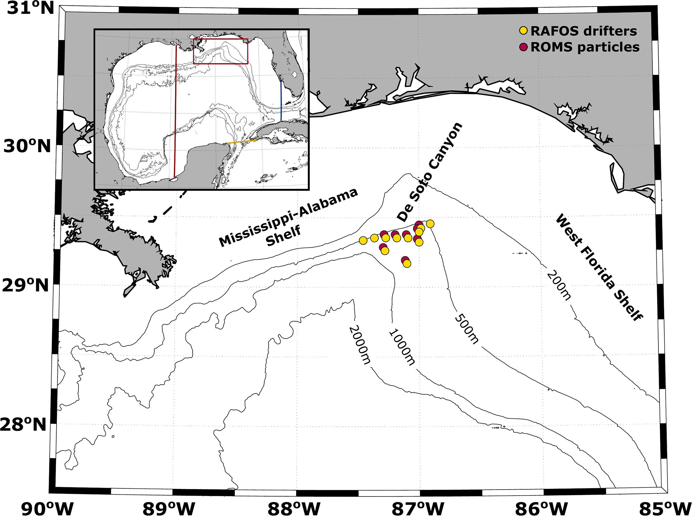
Figure 1 Map of the northeastern GoM with a map of the entire GoM in the top left-hand corner. The red rectangle on the full GoM map indicates the extent of the northeastern GoM (28°N–30°N, 85°W–90°W) as used during the SOM analysis. Red, yellow, and blue lines indicate the border between the eastern GoM and western GoM, Caribbean, and Atlantic, respectively, for the particle ending location calculation in Section 3.4 and Figure 12. Isobaths are shown in black at 200, 500, 1,000, and 2,000 m. Yellow and red circles indicate RAFOS drifter and ROMS virtual particle deployment locations, respectively.

Position fixes were obtained three times per day in order to resolve higher frequency motion. Apparent in some tracks is small-scale motion that are resolved inertial oscillations. In general, the accuracy of the position is expected to be about 1–2 km, although it can be worse at times when the float has a poor position relative to the sound sources or when it lies in a sound shadow. Sources were deployed to ensure tracking within DSC itself, which means other distant locations were less well covered with acoustic RAFOS signals.

Float deployments close to the seafloor, here the continental slope, are particularly risky since small ballasting errors of a few grams can translate into many meters of depth change, and touching a muddy bottom can change the weight and lead to failure. Due partly to this effect, of the 36 drifters deployed, 20 returned usable data, producing a total of 3,663 float-days of data. See Hancock and Speer (2013) for the full float report and Speer (2013) for the data.

All RAFOS floats are used when calculating the pseudo-Eulerian flow field in DSC. As most of the floats had left DSC after 100 days, we used only the first 100 days of RAFOS float data. For the capture and release of RAFOS floats by eddies, however, we focus on the trajectories of five specific RAFOS floats, which were captured by two eddies in DSC.

2.2 ROMS model output

Initially, this ROMS simulation was developed to provide the background solution for a 4DVAR data assimilative run to generate a GoM ocean reanalysis product. For this study, we employ 4 years of daily mean output from the free-running version, which is used to investigate the effect of eddies on virtual particle spreading and pathways within the eastern GoM.

ROMS is a 3D primitive equation ocean model employing hydrostatic and Boussinesq approximation (see Shchepetkin and McWilliams (2005); Shchepetkin and McWilliams (2009) and www.myroms.org for a full description of the model). The model is applied to the GoM and part of the Caribbean Sea using a grid with ~5 km horizontal resolution. It contains 327 × 375 computational cells and 36 vertical levels, extending from 97.7°W to 79°W and from 15.6°N to 30.54°N (Maslo et al., 2020; Morey et al., 2020). A nonlinear, free running (i.e., no data assimilation) simulation was integrated with forcing from 2010 to 2014 (Maslo, 2020). The bathymetry combines information from the “General Bathymetric Chart of the Oceans” (GEBCO), data from NOAA, proprietary data from PEMEX, and other observations collected during several cruises performed by the Ensenada Center for Scientific Research and Higher Education (CICESE). The need to smooth the bathymetry to avoid pressure-gradient–associated errors is a well-known problem of sigma coordinate models and can have an impact on the simulated deep and near-bottom circulations. To minimize this problem, an interactive method was used (Sikiric et al., 2009), where smoothing is only applied to the locations where spurious bottom currents generated by pressure gradient errors are observed. This method preserves a good representation of bathymetric features important to this study, such as the shelf break and DSC.

Hourly atmospheric forcing is provided by the Climate Forecast System Reanalysis (CFSR) (Dee et al., 2014). A bulk formulation scheme was used to calculate the heat, water, and energy fluxes at the surface (Fairall et al., 1996). The contribution from 21 rivers was included as point sources in the model domain. Daily measured water flux values provided by the U.S. Geological Survey (USGS) are used for the Mississippi and the Atchafalaya rivers, while climatological values reproducing the annual cycle are used for the Mexican rivers. In addition, 11 tidal constituents obtained from the Oregon State University TOPEX/Poseidon Global Inverse Solution (TPXO) (Egbert and Erofeeva, 2002) were introduced as a separate spectral forcing at the boundaries to the free surface and barotropic velocity, and as tidal potential at every grid point.

Initial and daily open boundary conditions are obtained from the “Global Eddy Permitting Ocean Reanalysis” 2 version 3 by Mercator Ocean—GLORYS2v3. Clamped conditions are applied at the southern and eastern boundaries, while a combination of radiative boundary conditions with nudging towards the GLORYS results is used at the northern boundary. Though the model is forced by prescribed surface and boundary conditions for the years 2010–2014, the fact that this simulation is not constrained by data assimilation means that the interior circulation features (e.g., the Loop Current and eddy field) behave stochastically and are not expected to replicate actual conditions from 2010 to 2014 (in the remaining text, reference to the simulation time periods will indicate the time periods of model forcing).

The ROMS hydrodynamics for this simulation was validated by Estrada-Allis et al. (2020) and Maslo et al. (2020), using velocity measurements from moorings and Lagrangian observations. This simulation was also compared to output from two additional numerical simulations, the Massachusetts Institute of Technology general circulation model (MITgcm) and the Hybrid Coordinate Ocean Model (HYCOM), over the same time period (Morey et al., 2020). Results demonstrated that ROMS was able to produce realistic surface and deep circulation in the GoM.

Virtual particle tracking in the ROMS simulation was done offline using the Dormand–Prince method (Dormand and Prince, 1980; Kimura, 2009). Since our primary interest is to supplement our sparse RAFOS results, all virtual particles are forced to stay at 400 m similar to our RAFOS deployment. Virtual particles were seeded daily at eight of the 11 RAFOS deployment locations (Figure 1) and advected horizontally for a year, using daily mean horizontal velocities from the ROMS simulation result. Due to RAFOS deployments occurring close to the slope and the horizontal ROMS model grid spacing employed, three of the RAFOS deployment locations were in water shallower than 400m and could not be used. Output was in the format of daily latitude and longitude positions for each virtual particle (see Maslo, 2020, for data). To validate the accuracy of virtual particle tracking, we subsampled ROMS virtual particles released in May 2012 and compared them to the RAFOS floats deployed in the same timeframe. Of the 248 virtual particles deployed, 20 were chosen at random, for 1,000 realizations. Both RAFOS floats and ROMS virtual particles were binned into a geographical grid of 0.25° longitude by 0.125° latitude and subsequently counted. Despite ROMS being a free-running model, and therefore not replicating actual conditions from 2012, we have good agreement between the float data and the mean virtual particle output (Supplementary Figure S1). Based on this result, and previous validations of ROMS model circulation, we presume the model output to be acceptable for further analysis.

2.3 Self-organizing maps

The goal of our research is to extract particle dispersion patterns and analyze their temporal variations. To this end, we use SOM, developed by Kohonen (1982), Kohonen (1998); Kohonen (2001); Kohonen (2013) and Vesanto et al. (2000). The SOM method is an artificial neural network based on unsupervised learning that performs nonlinear cluster analysis by mapping high-dimensional data onto a two-dimensional output space. Unlike variance-preserving EOFs, SOM preserves topology and naturally orders patterns most closely matching the original dataset (Liu and Weisberg, 2005). In other words, the SOM network architecture can be stretched and twisted but not cut or folded, and nodes will preserve connections to neighboring nodes, though distances between them can change (Supplementary Figure S2). However, SOM requires a predefined network architecture, which leads to user subjectivity when defining map size and shape. Results from SOM can therefore be strongly dependent on the initial architecture and parameter choices. Despite this, SOM has found widespread use across various disciplines as a pattern recognition and classification tool (Kaski et al., 1998; Oja et al., 2003; Liu et al., 2006; Liu and Weisberg, 2011; Vilibic et al., 2015; Liu et al., 2016; Meza-Padilla et al., 2019). For an in-depth explanation of the SOM technique, including the training process and parameter choices for oceanography, we refer the reader to Liu et al. (2006); Liu et al. (2016).

In our study, the spatial and temporal analysis was based on 36-time steps (i.e., monthly composites of virtual particle distribution in the northeastern GoM from 3 years of ROMS model output, see Supplementary Figure S2) and 4,100 grid points (i.e., a geographical grid of 0.05° latitude by 0.05° longitude over the northeastern GoM, see Figure 1), respectively. In the first step of the SOM training process, nodes are distributed randomly on a two-dimensional space, based on the multidimensional input data (Supplementary Figure S2). Successive steps then proceed iteratively between input data and SOM, until the nodes approach the best representation of the input data. This is achieved by finding the best matching unit (BMU), defined as the minimum Euclidian distance between the node weights and original input data, after each iteration. The BMU and neighboring nodes are modified towards the input data, allowing similar patterns to be mapped closer together and dissimilar patterns farther apart. Supplementary Figure S2 illustrates the SOM process visually, where the input is a 2D array of monthly composites of virtual particle distribution and the output is N maps of virtual particle distributions.

Several SOM parameters controlling the initialization, iteration, and final output are tunable. Liu et al. (2006) suggested a set of SOM parameters for practical application based on their evaluation of the tool. We follow their suggestions on the parameter choice for initialization, learning rate, and neighborhood function. In addition, the user must specify the SOM map size, which is an empirical process determining how much detail is available for the analysis. This means a trade-off exists between compressing information into a manageable size and accuracy (Liu et al., 2006). We chose a rectangular grid with approximately 30 nodes, calculated using the following formula: $5x\sqrt{\text{number\hspace{0.17em}of\hspace{0.17em}samples}}$ [Vesanto et al. (2000)], and a hexagonal lattice to avoid directional preference (Kohonen, 2001). To determine the map grid arrangement, we used the ratio of the two largest eigenvalues of the input data to set the ratio of grid side lengths ([9 × 3]). The actual side lengths were then set such that their product approximated the number of nodes calculated above (i.e., 27). Sensitivity tests were performed with varying map grid arrangements, the number of nodes, and training length, where each scenario was run multiple times to ensure stability and consistency of the results. To further quantify the quality of our final maps, we used two error estimates provided by the SOM toolbox: average quantization error (QE) and topographic error (TE). The QE quantifies how much detail is being learned by the SOM, and TE measures the projection quality. For our analysis, QE and TE were 0.014 and 0.02, respectively, which indicate reliable maps. The SOM MATLAB Toolbox 2.0 by Vesanto et al. (2000) was used, which we downloaded from the Laboratory of Information and Computer Science at the Helsinki University of Technology (http://www.cis.hut.fi/somtoolbox).

3 Results

3.1 Eddies in DSC and the northeastern GoM

Five RAFOS drifters are captured by eddies in DSC, one transient cyclone moving with the background flow (Figure 2A) and another stationary anticyclone just south of the 1000-m-depth contour (Figure 2B). Drifter tracks are overlayed pseudo-Eulerian velocities (shown in dark pastel green), which were calculated on a geographical grid of 0.25° longitude by 0.125° latitude, using all RAFOS drifter tracks over their first 100 days. The transient cyclone captures one drifter (purple track in Figure 2A) within the upper part of DSC, close to the drifter deployment location, and travels southward with the background flow. As the cyclone enters an area with reduced background flow, it briefly captures two more drifters (red and black tracks in Figure 2A), before moving westward. Evident in the streamlines is the stationary anticyclone, which captures four of the drifters (red, black, green, and blue tracks in Figure 2B). Upon the drifters’ release from the stationary anticyclone, three continue westward (red, green, and black tracks), whereas one travels south (blue track).

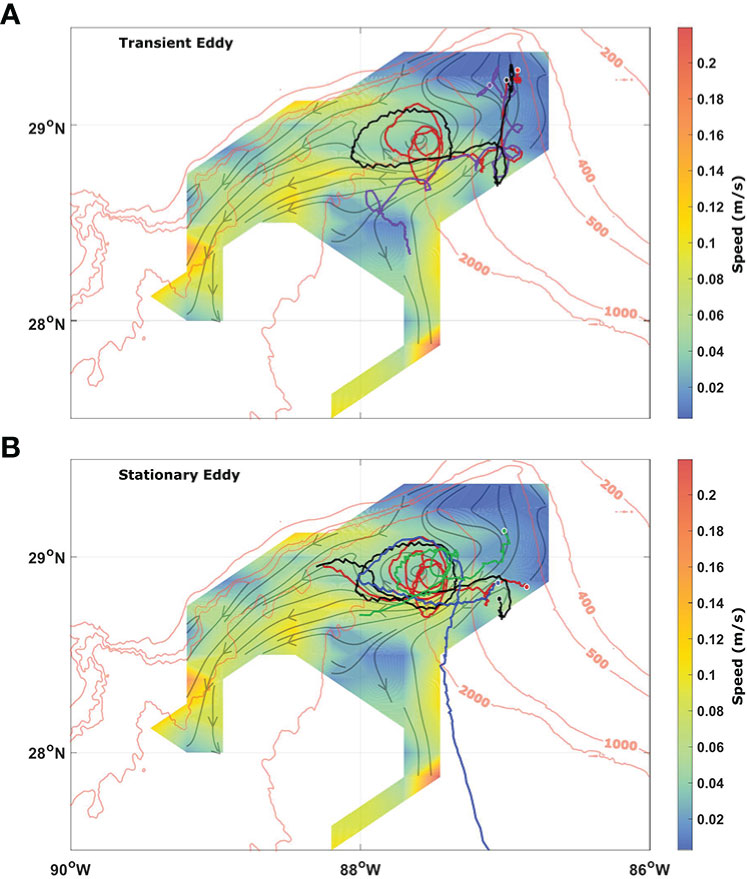
Figure 2 Tracks of RAFOS drifters captured by the (A) transient cyclonic eddy and (B) stationary anticyclonic eddy. A circle indicates the start of each track. Mean speed, calculated using all 20 RAFOS tracks over their first 100 days, is colored, with streamlines given in light green. Isobaths are shown in red. RAFOS drifters captured by the transient eddy are 1189 (red), 1194 (purple) and 1195 (black), and the stationary eddy are 1177 (green), 1189 (red), 1195 (black), and 1196 (blue).

Based on RAFOS trajectories, we estimated the transient cyclone to be O(10 km) in diameter and therefore too small to be detected by satellite remote sensing measurements, such as sea surface height and temperature anomalies. Although the stationary anticyclone is at the detection limit with a diameter of ~40 km, it is not distinguishable by satellite altimetry either. This could be because it is a subsurface eddy with weak surface expression. No other supplementary data, such as mooring arrays and/or hydrographic profiles, are available for this time period.

ROMS virtual particle tracks show similar structures throughout all five model years, with eddies ranging in size from O(10 km) to O(100 km) within the northeastern GoM. In fact, a stationary eddy is often seen at the base of DSC, in a similar location as that identified by the RAFOS floats data. Calculating velocities from the year-long virtual particle trajectories and binning these into a geographical grid (0.05° longitude by 0.05° latitude), we constructed monthly pseudo-Eulerian velocity fields for 2011–2013. These illustrate the presence of semistationary eddies in the northeastern GoM (Figures 3A, B). For transient eddies, single virtual particle trajectories show their presence in DSC (Figure 3C).

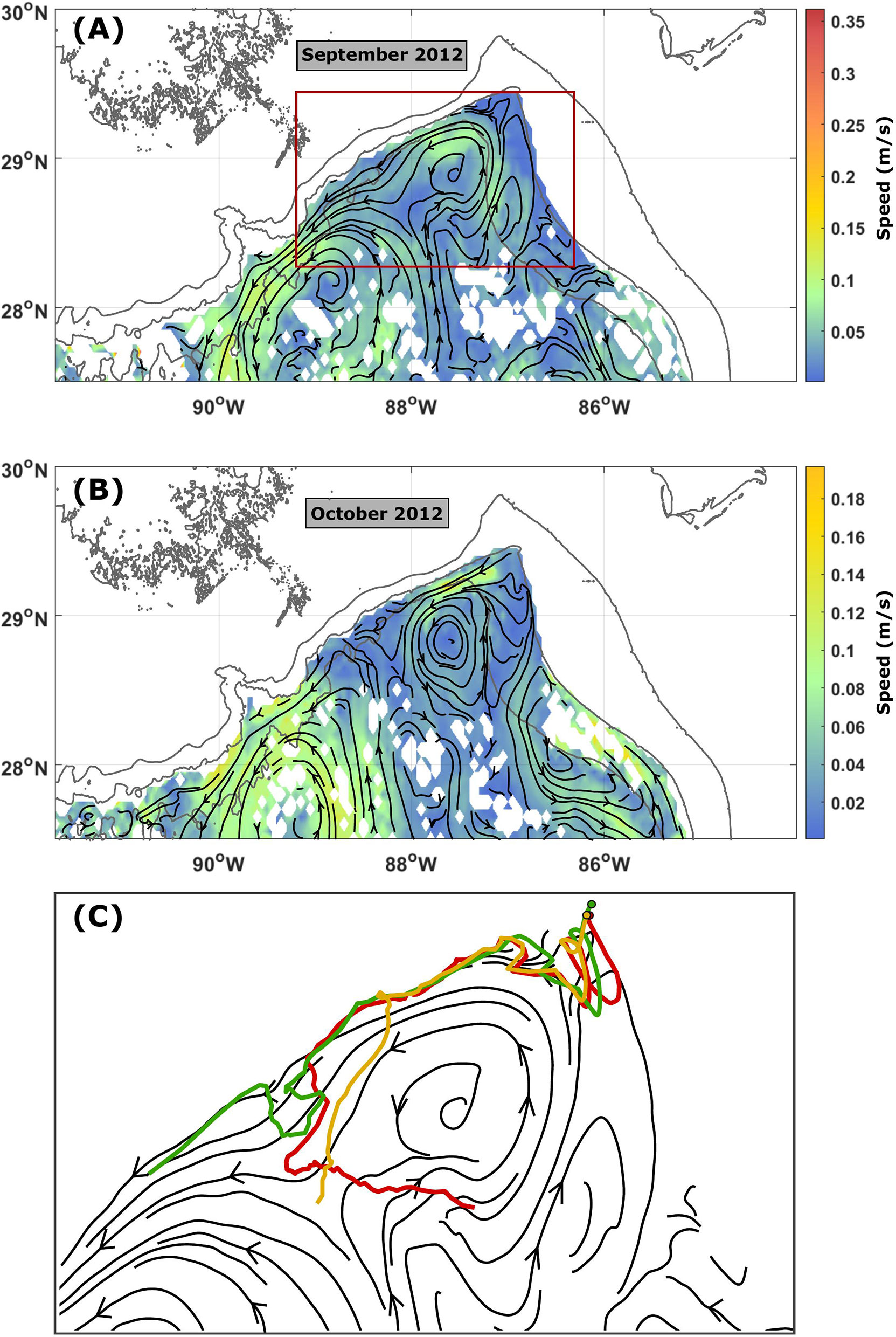
Figure 3 Pseudo-Eulerian velocity fields for (A) September 2012 and (B) October 2012, calculated from virtual particle velocities binned in a 0.05° × 0.05° geographical grid. Mean speed is colored, and streamlines are given in black. Isobaths are shown in dark grey. (C) The first 100-day tracks of three virtual particles deployed in September 2012 were superimposed onto streamlines from (A), where the red box in (A) indicates the area of (C). Circles indicate deployment locations.

3.2 Circulation in the northeastern GoM

The Loop Current System (LCS) wields a significant influence on subsurface circulation in the northeastern GoM and DSC. Monthly pseudo-Eulerian velocity fields, calculated from year-long virtual particle trajectories and binned into a geographical grid of 0.05° ×0.05°, show strong eastward along-slope flow in 2010 and 2011 (Figure 4), corresponding to years dominated by a LCS that extends northwestward toward the Mississippi Canyon (Liu et al., 2016). Hamilton and Lee (2005) observed a similar correlation between LSC location and along-slope flow direction, attributing it to potential vorticity conservation. During late spring and early summer of 2011, the LCS extends northeastward toward DSC, which is clearly seen in the monthly pseudo-Eulerian velocity field (Figure 4). Again, Hamilton and Lee (2005) found evidence of a Loop Current Frontal Eddy intruding over the slope, affecting upper-layer along-slope flow patterns. In contrast, 2012’s flow field is much weaker, with an along-slope flow predominantly directed westward (Figures 3A, B). Multiple eddies were also present throughout the northeastern GoM. Although 2012 saw the shedding of two Loop Current Eddies (LCE), these moved quickly westward, and the Loop Current (LC) was retracted for large portions of the year (Liu et al., 2016). The flow in 2013 was a mixture between 2010–2011 and 2012, with the mean along-slope flow equally directed eastward and westward (not shown).

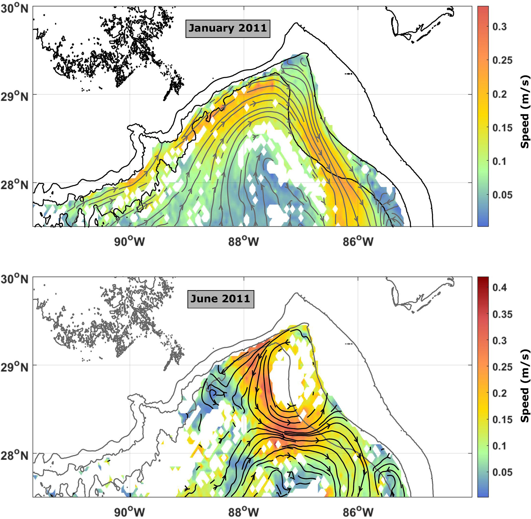
Figure 4 Pseudo-Eulerian velocity fields for (top) January 2011 and (bottom) June 2011, calculated from virtual particle velocities binned in a 0.05° × 0.05° geographical grid. Mean speed is colored, and streamlines are given in black. Isobaths are shown in dark grey.

Eddy activity in the northeastern GoM is evident through the monthly pseudo-Eulerian velocity fields (Figures 3, 4). However, to better quantify the interannual variability in eddy activity, we calculated the yearly mean and eddy kinetic energy (MKE and EKE, respectively) for 2011–2013, using the following formula:

Here, the bar denotes the time mean, and N is the number of months. The calculation was performed for each 0.05° ×0.05° grid box within the northeastern GoM over 12 months. To identify the persistence of eddy activity, Figure 5 shows the ratio of EKE to the total kinetic energy (EKE+MKE) as a percentage for each year. Elevated levels of EKE along the West Florida Shelf (WFS) and Mississippi–Alabama slopes in 2011 are most likely due to variability in the along-slope flow. Previous work has suggested several causes for this variability, such as wind forcing, the LCS, and eddy activity (Wang et al., 2003; Hamilton and Lee, 2005; Teague et al., 2006; Carnes et al., 2007; Hallock et al., 2009). The year 2011 also exhibits high EKE along 87°W and 88°W, which is probably due to the northward extension of the LCS in late spring and early summer of that year. In comparison, 2012 has elevated EKE levels throughout most of the northeastern GoM, with noticeably lower values on the WFS and Mississippi–Alabama slopes. This correlates to monthly pseudo-Eulerian velocity maps, which display abundant eddy activity within the whole northeastern GoM during most months. Similar to the monthly pseudo-Eulerian velocity fields, 2013 exhibits high EKE both along the slopes and within the interior, indicating a mixture of high eddy activity and variable along-slope flows.

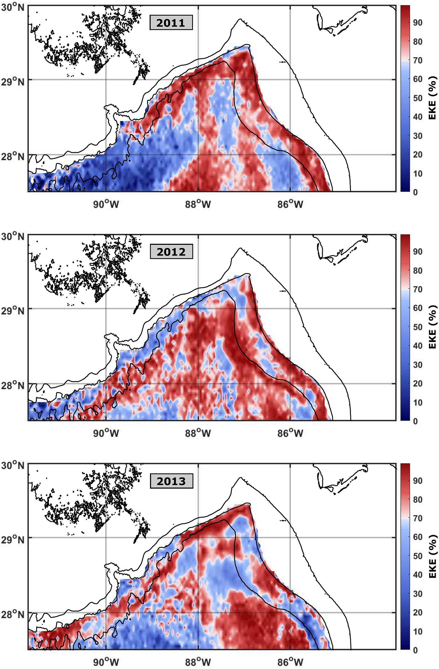
Figure 5 Ratio of EKE to total kinetic energy (EKE+MKE) in each grid cell, represented as a percentage for 2011 (top), 2012 (middle), and 2013 (bottom) in the northeastern GoM. EKE and MKE are calculated from virtual particle velocities binned in a 0.05° × 0.05° geographical grid, for each year separately. Isobath is shown in black.

3.3 Virtual particle dispersion in the northeastern GoM

To investigate pathways out of DSC and the northeastern GoM, we again use the year-long virtual particle trajectories and 0.05° ×0.05° geographical grid, counting the number of virtual particles in each grid cell for each month, normalized by the total number of virtual particles in the basin. Figure 6 shows results from 2 months with abundant (Figure 6A) and marginal (Figure 6B) eddy activity, respectively. When there is considerable eddy activity in the northeastern GoM (defined here as north of 28°N), virtual particles are dispersed within the entire northeastern basin, such as in October 2013 (Figure 6A). However, whenever eddy activity is at a minimum, virtual particles are more confined to the slopes bordering either the WFS (Figure 6B) or the Mississippi–Alabama Shelf, dependent on the predominant direction of the along-slope flow.

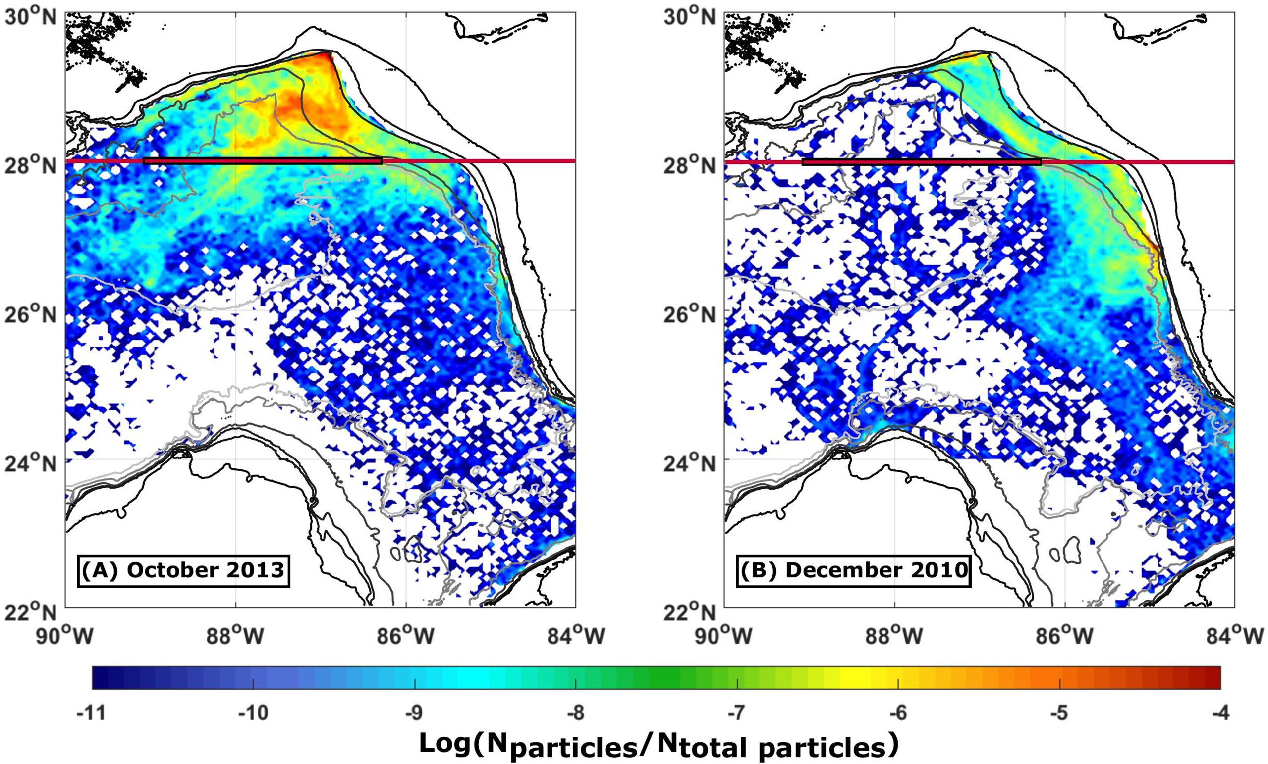
Figure 6 Density of virtual particles in each grid cell normalized by the total number of virtual particles in the domain, represented on a log scale for (A) October 2013 and (B) December 2010. Isobaths are shown with black and gray lines. The red line indicates 28°N, and the black outlined section indicates water depths greater than 1,500 m along 28°N.

To further illustrate these pathways out of the northeastern GoM and how they fluctuate in time, we explore the longitude at which virtual particles move south across 28°N (red line in Figure 6) as a function of time (Figure 7). There are significant differences both within and between years. During the latter part of 2010, most virtual particles exited east of 87°W, whereas 2012 reveals the opposite flow pattern, with most virtual particles exiting west of 87°W. If we define 86.5°W–89°W as the interior basin with a water depth greater than 1,500 m (the black outlined portion of the red line in Figure 6) and consider the total number of virtual particles crossing 28°N at that location, we can examine the cumulative effect of variable eddy activity (Figure 7A). Although we see singular months with a sizable particle density crossing 28°N in the interior basin during 2010–2011, half of the months exhibit particle densities less than the lowest values found in 2012–2013. On a yearly timescale, 2010–2011 had a third less virtual particles crossing 28°N in locations where the water depth is greater than 1,500 m, compared to 2012–2013 (Figure 7A). In other words, more virtual particles were confined to slope regions during 2010–2011 than in 2012–2013.

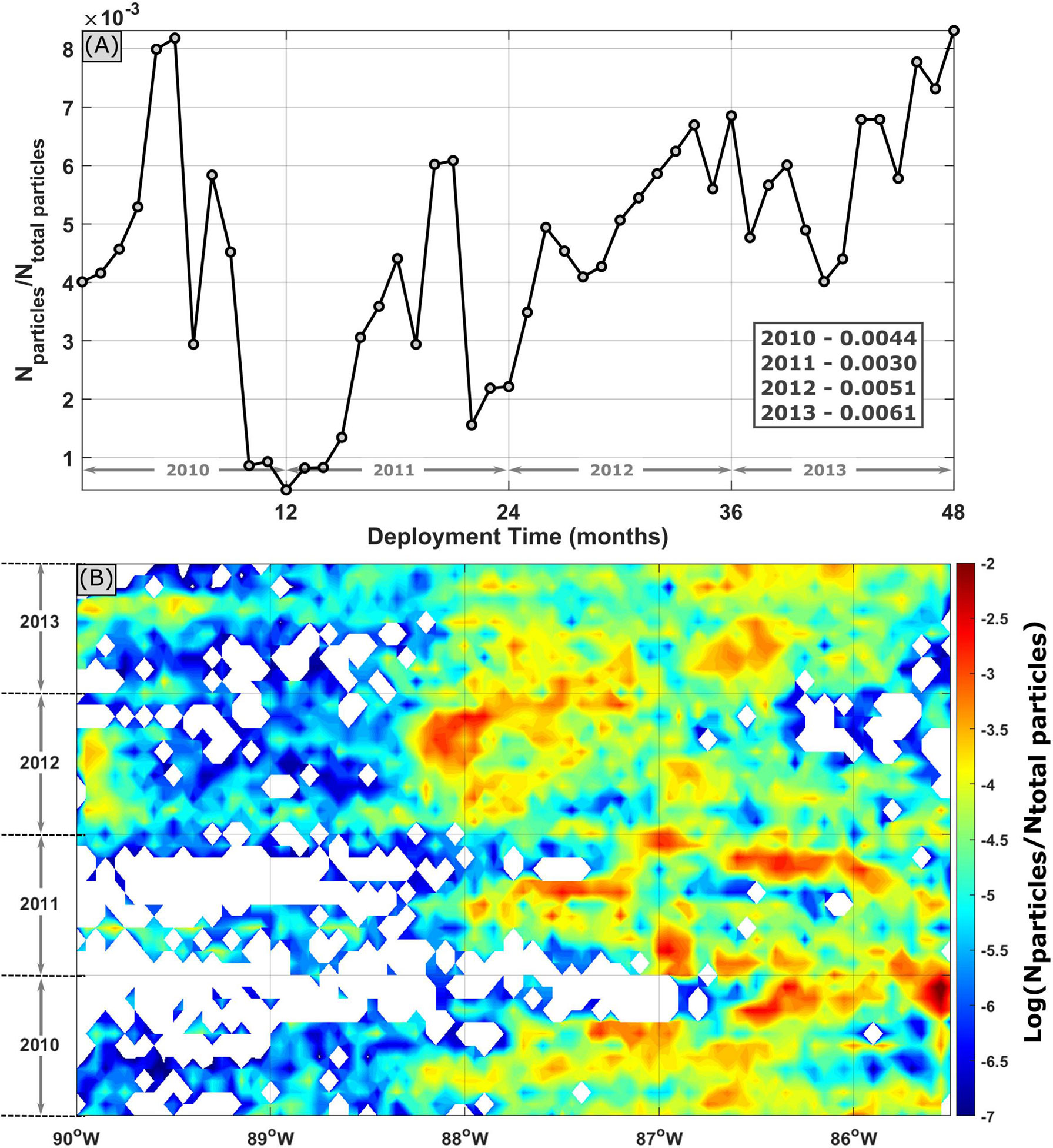
Figure 7 (A) Virtual particle density, normalized by the total number of virtual particles in the domain, moving south across 28°N in water depths greater than 1,500 m (defined as 86.5°W–89°W, the section of the red line at 28°N outlined in black in Figure 6), as a function of months from deployment. The inset box gives the mean for each year. (B) Virtual particle density, normalized by the total number of virtual particles in the domain, moving south across 28°N as a function of longitude and time, is represented on a log scale.

How are these particle pathways connected to the dynamics occurring in the northeastern GoM? To answer this question, we use the SOM method to extract particle dispersion patterns over the model years 2011–2013 in the area 28°N–30°N, 85°W–90°W (red box in Figure 1). In order to reduce errors associated with the SOM technique, we settled on a [9 × 3] hexagonal grid of nodes. SOM maps (i.e., nodes) and BMUs (i.e., the SOM map that best describes the dataset at each time step) associated with each of the model years 2011, 2012, and 2013 are grouped in separate figures (Figures 8–10), whereas the full map of nodes in the hexagonal grid can be found in the Supplementary Material (Supplementary Figures S3 and S4). Six of the SOM maps never occurred during model years 2011–2013 (maps 8, 11–14, and 17). Of the remaining SOM maps, we notice differences between 2011 and 2012–2013. During 2011, we predominantly observed variations of eastward flow along the WFS and reduced eddy activity occurring in maps 1, 18, 19, 20, and 21 (Figure 8). A composite of these SOM maps illustrates this exiting flow pattern (Figure 11A), which occurs 58% of the time in 2011. This agrees with the EKE (Figure 5) and monthly pseudo-Eulerian velocity fields (Figure 4) for 2011, which show reduced eddy activity and increased along-slope variability. In contrast, westward flow along the Mississippi–Alabama shelf dominates in 2012 (maps 4, 6, 16, 25, and 26), with an increased eddy activity in the northeastern GoM (Figure 9). The year 2013 shows similar increased eddy activity as 2012, though with a mixture of eastward and westward along-shelf flow patterns (Figure 10). Again, we created a composite of the SOM maps where mixing occurs in 2012–2013 (this will be termed “eddy mixing”), shown in (Figure 11B). Eddy mixing occurs 75% of the time during 2012–2013, which is corroborated by the EKE (Figure 5) and monthly pseudo-Eulerian velocity fields (Figure 3) for 2012–2013. We observe a similar pattern in particle recirculation, with increased virtual particles within 3 km of their initial deployment location during 2012–2013, compared to 2010–2011 (Table 1).

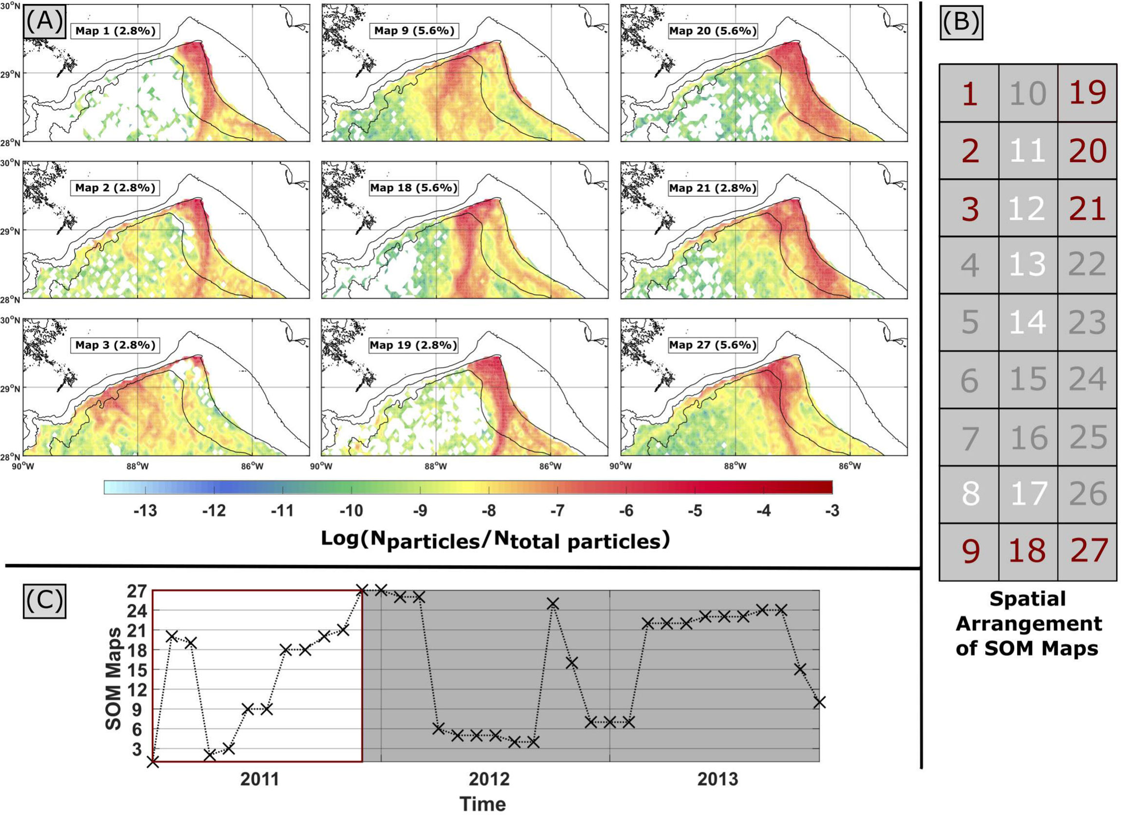
Figure 8 (A) SOM maps presenting virtual particle density in each grid cell, normalized by the total number of virtual particles in the domain, for 2011, represented on a log scale. Isobaths are shown in black. (B) The user specified spatial arrangement of SOM maps for the analysis, where the white, red, and gray numbers represent SOM maps that never occur, occur in 2011, and do not occur in 2011, respectively. (C) The BMU for each month, where the white area signifies 2011.

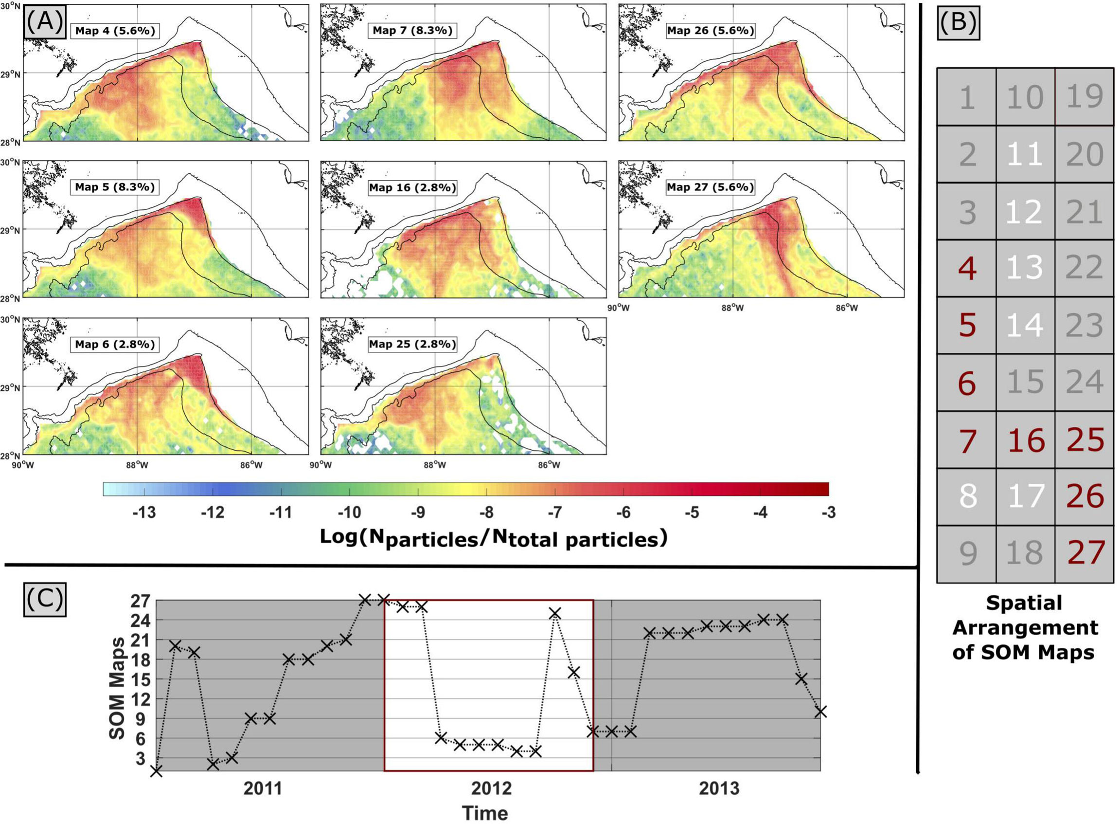
Figure 9 Same as Figure 8, but for 2012.

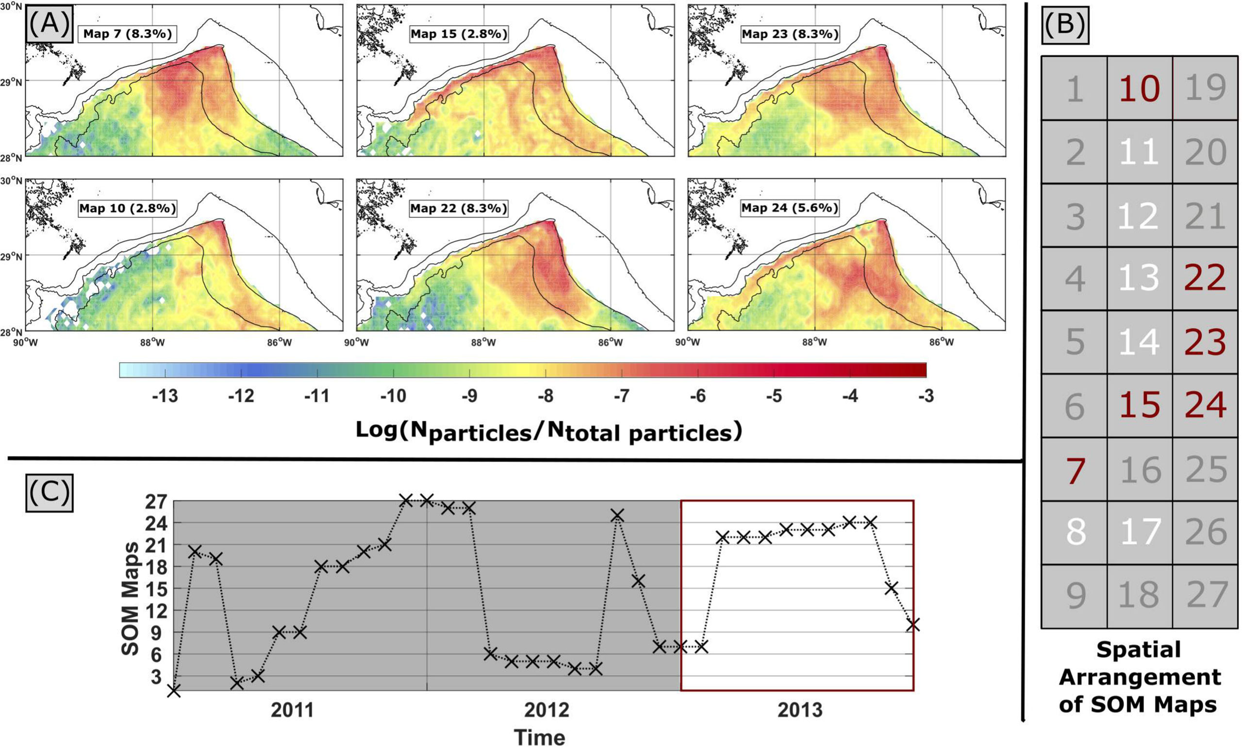
Figure 10 Same as Figure 8, but for 2013.

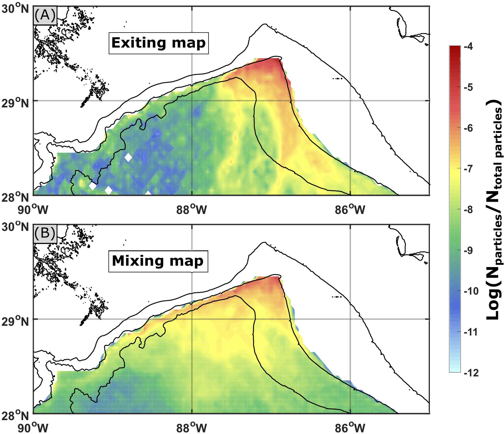
Figure 11 Composite of SOM maps to show typical exiting (A) and eddy mixing (B) flow patterns. Exiting and eddy mixing flow patterns are calculated as a mean of SOM maps [1, 18–21] and [4–7, 23–24, 26–27] (see Figures 5–7), respectively. The exiting flow pattern occurred 58% of the time in 2011, whereas the eddy mixing flow pattern occurred 75% of the time in 2012–2013. Isobaths are shown in black.

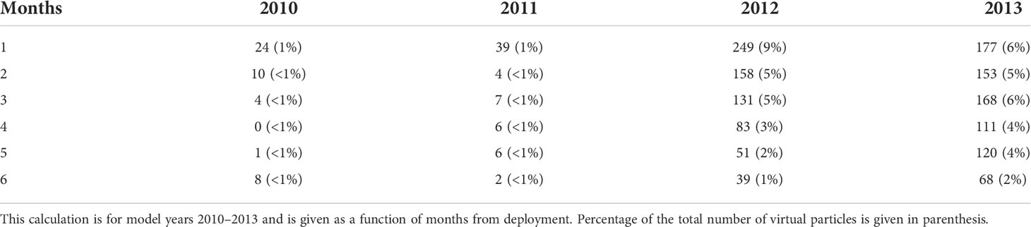
Table 1 Number of ROMS virtual particles within 3 km of their deployment sites.

3.4 Virtual particle residence time in the eastern GoM

Given the above variations in virtual particle pathways exiting DSC, how do these control (1) the Lagrangian dispersion of virtual particles out of the eastern GoM and (2) virtual particle residence times in the eastern GoM? To answer both questions, we expand our view and investigate virtual particles that leave the eastern GoM. For this analysis, we divide our area into four sections: (1) the Atlantic (east of 82°W), (2) the western GoM (west of 92°W), (3) the Caribbean (south of 22°N), and (4) the eastern GoM (see Figure 1). Once a virtual particle leaves the eastern GoM, it is considered to be at its final destination. At the end of a virtual particle’s 1-year drift, if it has not exited the eastern GoM, this is considered its final destination. Approximately 3% of virtual particles re-entered the eastern GoM, almost exclusively from the western GoM, over the entire 4 years. Since we are primarily concerned with virtual particle pathways within and out of the eastern GoM, excluding the re-entry of virtual particles should not affect our analysis. We also want to note that, though the natural divide between the eastern and western sections of the GoM is located around 90°W, several virtual particles entering the region between 90°W and 92°W reversed direction before crossing 92°W and traveled back into the eastern GoM. To ensure these virtual particles were not identified as entering the western GoM, we set the divide at 92°W. Figure 12 shows virtual particles exiting the eastern GoM as a function of deployment month, throughout the model years 2010–2013. An increase in Lagrangian dispersion into the Atlantic (blue line) occurs during model years 2010–2011, whereas the reverse happens in model years 2012–2013 (purple line). Regarding the western GoM, 2012 sees a modest increase in Lagrangian particle dispersion into the western GoM (red line). We observe a similar distinction between 2010–2011 and 2012–2013 in virtual particle residence times (Figure 13), with an average 50-day shorter mean residence time in 2010–2011 compared to 2012–2013.

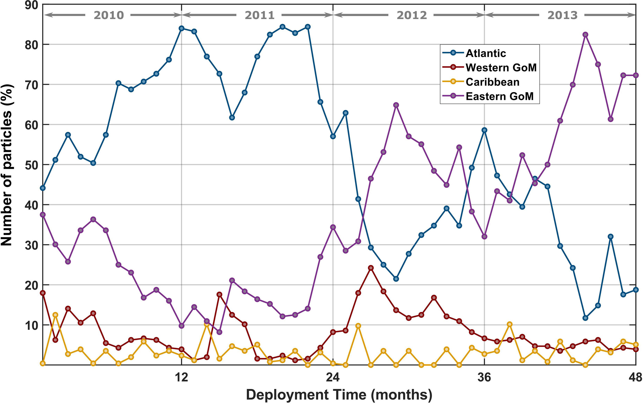
Figure 12 ROMS virtual particles’ final destination as a function of deployment month, divided into the Atlantic (blue line), western GoM (red line), Caribbean (yellow line), and eastern GoM (purple line). Regions are defined as follows: Atlantic is east of 82°W, western GoM is west of 92°W, the Caribbean is south of 22°N, and eastern GoM is within the bounds of 22°N–30°N and 82°W–92°W (see Figure 1). Once a virtual particle exits the eastern GoM into one of the three locations, that location is considered its final destination. If after a virtual particle’s 1-year drift it has not exited into one of the three locations, the eastern GoM is considered its final destination.

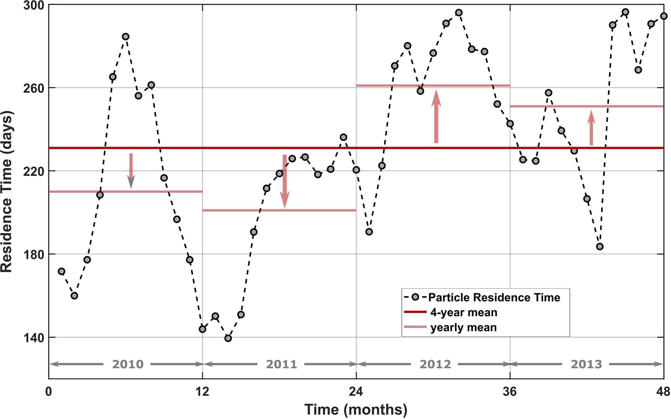
Figure 13 Residence time (days) of virtual particles in the eastern GoM as a function of deployment month. The solid red line shows the 4-year mean, whereas the light red lines show yearly means with arrows indicating offset from the 4-year mean.

4 Discussion

As shown analytically by Flierl (1981) and numerically by Shapiro et al. (1997), a variable background flow will change an eddy’s trap zone, allowing it to capture and release particles throughout the eddy’s lifetime. This means that the time a particle travels within an eddy is based on how close that particle is to the eddy’s core compared to the strength of the background flow. For a highly variable background flow, individual particles can be mixed along an eddy’s path through the capture-and-release principle, instead of being transported with the eddy until it decays. Although it is hard to quantify this type of mixing on a large scale, it can become important in areas where flow is highly constrained, such as DSC and the northeastern GoM. Mean flow at 400 m in DSC and the northeastern GoM is often confined to the continental slope, flowing either eastwards or westward along isobaths (Teague et al., 2006; Carnes et al., 2007; Hamilton et al., 2000; Hamilton and Lee, 2005). The along-isobath flows parallel to the West Florida and Mississippi–Alabama shelves transport particles to exit pathways into the Atlantic and western GoM, respectively. These exit pathways are located (a) at the western edge of the Florida Straits and (b) southwest of the Mississippi Canyon (Figure 14). RAFOS drifter tracks (Figure 2) illustrated how eddies can capture drifters and transport them across isobaths into the basin interior. Based on novel Lagrangian observations we postulate that eddies transport particles away from depth-constrained along-slope pathways, affecting their dispersion and residence times in the eastern GoM.

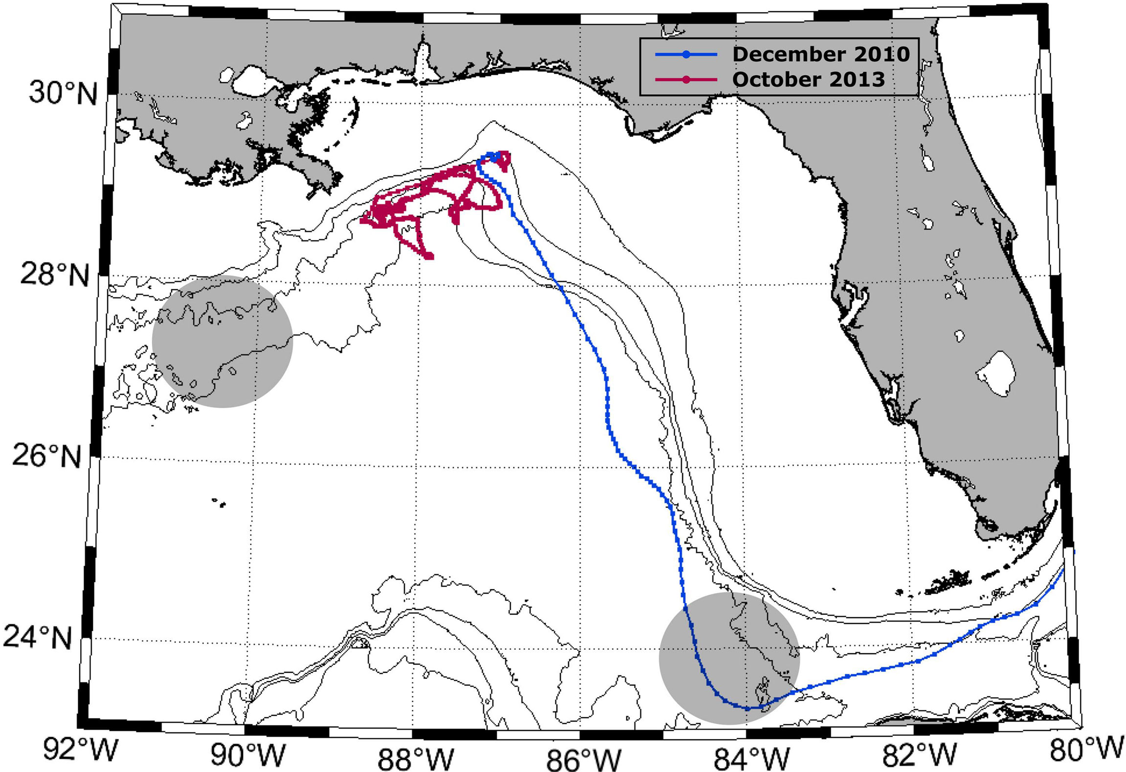
Figure 14 Example virtual particle tracks for times with reduced (blue) and increased (red) eddy activity in the northeastern GoM. Gray-shaded areas located at the western edge of the Florida Straits and southwest of Mississippi Canyon denote particle exit points into the Atlantic and western GoM, respectively. Isobaths and coastlines are shown in black.

To draw together the larger-scale consequences of the eddy ejection effect, let us assume minimal eddy activity in the northeastern GoM, which means that flow at 400 m depth in DSC will primarily occur along isobaths. If this along-slope flow is directed eastward, it will transport virtual particles to the western edge of the Florida Straits where a majority of floats will exit into the Atlantic (Figures 11A, 12). Years with reduced eddy activity would see an increase in virtual particles exiting the eastern GoM, as well as a reduction in their residence times within the eastern GoM. This is consistent with model output from the years 2010–2011 (Figures 4, 5), which shows (a) an increase in the number of virtual particles exiting the northeastern GoM confined to the continental slope (Figures 7, 8), (b) an increase in the number of virtual particles exiting the eastern GoM into the Atlantic (Figure 12), and (c) a decrease in virtual particle residence time in the eastern GoM (Figure 13). However, if eddies populate the northeastern GoM, some virtual particles will be captured and transported away from the along-slope flows and into the basin interior (Figures 11B, 12). This will increase virtual particle residence times in the eastern GoM as well as reduce the number of virtual particles exiting the eastern GoM within their 1-year drift. Again, this is consistent with model output from the years 2012 to 2013 (Figures 3, 5), with (a) a spread in longitudes where virtual particles exit the northeastern GoM (Figures 7, 9, 10), (b) a decrease in the number of virtual particles exiting the eastern GoM (Figure 12), and (c) an increase in virtual particle residence time in the eastern GoM (Figure 13). Examples of virtual particle tracks for times with reduced and increased eddy activity in the northeastern GoM are shown in Figure 14.

Given the above modeling results, the LCS and eddies seem to dominate subsurface circulation in the northeastern GoM. It is therefore not surprising that neither virtual particle pathways nor virtual particle residence times show any significant seasonal signal throughout the model years 2010–2014, as both are dependent on the total flow at any one point. There is, however, significant interannual variability, which better reflects the temporal behavior of the LCS. In fact, Wang et al. (2003) established a connection between the location of the northern LC front and near-surface flows over the lower Alabama slope. It is thought that part of the eddy activity in the northeastern GoM is generated by the LCS and advected into the region (Hamilton et al., 2000; Ohlmann et al., 2001; Ohlmann and Niiler, 2005; Hamilton and Lee, 2005; Hamilton, 2007). There does, however, seem to be a preference for eddies along the Mississippi slope, which could be a reflection of bathymetric structures, such as canyons and headlands, in this region. Such structures could force the along-slope current to meander, setting the stage for eddy generation through potential vorticity conservation. Since the LCS seems to affect the along-slope current’s strength and direction, this could directly affect eddy generation in this area. DSC has also been suggested as a site for local eddy generation due to sharp bends in the bathymetry (Weisberg et al., 2005).

Although subsurface flow in the northeastern GoM is typically found to be constrained by bathymetry at depth, five RAFOS drifters showed across-isobath movement. If eddies can pull particles from preferred along-slope pathways and into the interior, this will modulate particle dispersion (Figure 14). Thus, the magnitude of eddy activity in the northeastern GoM not only affects particle dispersion in the northeastern GoM but residence times in the eastern GoM as well.

Similar to subsurface drifter data, surface float data in the northeastern GoM, notably from the Surface Current and Lagrangian Drift Program (SCULP II) and the Grand Lagrangian Deployment (GLAD), shows mesoscale eddies as an important dynamical feature affecting cross-slope flow (Ohlmann and Niiler, 2005; Poje et al., 2014; Hamilton et al., 2015; Mariano et al., 2016) and dispersion (LaCasce and Ohlmann, 2003; Poje et al., 2014). LaCasce and Ohlmann (2003) found evidence for super diffusive dispersion in surface waters using the SCULP II floats, with exponential growth over length scales of 50 km. Their results suggested a spectral continuum of eddies affecting relative dispersion, where eddies of a given scale affected dispersion of the same scale. Both LaCasce and Ohlmann (2003) and Ledwell et al. (2016) found evidence of exponential stretching of tracers into long filaments, despite the study sites being located at the surface and 1,100 m depth, respectively. Near DSC, surface velocity seems to be set by a combination of wind forcing, the energetic eddy field, and the northern LC front (Wang et al., 2003; Hamilton and Lee, 2005; Mariano et al., 2016). Given this complex flow pattern, float tracks are heavily dependent on the dynamical features present and, consequently, their deployment conditions. In fact, Poje et al. (2014) found residence times in DSC could vary from a week to a month, due to this. Both surface floats and subsurface floats observe transient and stationary eddy features in DSC during their deployment (Hamilton and Lee, 2005; Ohlmann and Niiler, 2005; Hancock and Speer, 2013). The eddy activity in DSC seems to homogenize the upper-layer potential vorticity, removing dynamical barriers for cross-slope flow (Hamilton and Lee, 2005). However, whereas surface floats move offshore and into the Atlantic within 90 days, subsurface virtual particles take an average of 230 days to reach the Atlantic (Figure 13). This difference is possibly due to the lack of direct wind forcing on the subsurface virtual particles.

The northeastern GoM, which includes the Mississippi–Alabama and WFS shelves and slopes as well as DSC, exhibits complex ecosystems defined by high biodiversity and substantial biomass. An important aspect of this is the plume of nutrient-rich low-salinity water from the Mississippi River outflow. Morey et al. (2003a), Morey et al. (2003b) and Schiller et al. (2011) showed using numerical simulations that this low salinity water can be transported off the shelf through a combination of wind forcing and mesoscale eddies in DSC. DSC is a natural pathway for particle transport across the slope, connecting deeper waters with shelf waters along the northeastern GoM. Hamilton and Lee (2005) found evidence of smaller-scale eddies near DSC, which could cause strong cross-slope velocities. These cross-slope velocities thus control the transport of contaminants, such as subsurface oil from the Deepwater Horizon accident, onto the slope and shelf, as well as nutrient-rich Mississippi plume waters off the shelf.

Regions such as DSC, with a highly variable background flow and considerable eddy activity, are likely to spread particles over a substantial area due to the capture-and-release effect of eddies. Eddies can draw tracers into long filaments, which preserves maximum concentrations and gradients better than simple lateral diffusion. Realizing this can aid in containment strategies for future anthropogenic contamination spills.

Although our research has shown the importance of eddy activity in the northeastern GoM, specifically with regard to particle dispersion and residence times, it suffers from several limitations. The main shortcomings are as follows: (a) the length of the numerical simulation, (b) virtual particle deployment confined to a singular location, and (c) a virtual particle’s inability to move vertically in the water column. The length of our simulation was 5 years, with 4 years of virtual particle tracking. With longer simulation times, for example, 20 years, more robust statistics would be available for the analysis. In particular, the SOM method would greatly benefit from an order of magnitude increase in timesteps. As the model output was intended to expand upon the float data, the virtual particle deployment and tracking were configured with the RAFOS experiment in mind. For more comprehensive statistics, particularly relating to the movement of particles into and through DSC, deployment locations should have included sites exterior to DSC, such as its western and eastern flanks. In addition, virtual particles were unable to move vertically in the water column, again to replicate the RAFOS experiment. Understanding the three-dimensional movement of particles in DSC, in particular the connection between the shelf, slope, and deep waters, is beneficial to ecosystem research on the northeastern continental shelf and slope. Future research in the northeastern GoM could start by remedying these noted shortcomings and thus forming a more coherent picture of the dynamics controlling subsurface flow, its variability, and its connectivity to the slope and shelf.

Data availability statement

The datasets presented in this study can be found in online repositories. The names of the repository/repositories and accession number(s) can be found below: https://deep-c.coaps.fsu.edu/data (Deep-C Consortium), and https://gfdi.fsu.edu/research/research-data (Geophysical Fluid Dynamics Institute, FSU).

Author contributions

CH tracked and analyzed the RAFOS float data, analyzed the ROMS virtual particle output, created figures, and wrote the manuscript. KS supplied the RAFOS float data and contributed to the analysis and editing of the manuscript. JS supplied the ROMS model output and contributed to manuscript editing. SM contributed to the analysis methods and editing of the manuscript. All authors listed have made a substantial, direct, and intellectual contribution to the work and approved it for publication.

Funding

This work was funded by the National Academy of Sciences through the Gulf Research Program grant award 2000006422, and GoMRI and the Deep-C consortium through award SA-12-12/GoMRI-008.

Conflict of interest

Author JS is employed by MetOcean Solutions Ltd.

The remaining authors declare that the research was conducted in the absence of any commercial or financial relationships that could be construed as a potential conflict of interest.

Publisher’s note

All claims expressed in this article are solely those of the authors and do not necessarily represent those of their affiliated organizations, or those of the publisher, the editors and the reviewers. Any product that may be evaluated in this article, or claim that may be made by its manufacturer, is not guaranteed or endorsed by the publisher.

Supplementary material

The Supplementary Material for this article can be found online at: https://www.frontiersin.org/articles/10.3389/fmars.2022.949338/full#supplementary-material

Supplementary Figure 1 | Dominant pathways represented by number of floats/virtual particles in each grid cell (0.25^o longitude x 0.125^o) on a log₁₀ scale for (top) RAFOS floats and (bottom) ROMS virtual particles deployed during May 2012. For this calculation, floats/virtual particles were not permitted to re-enter the northeastern box once they have exited it. Isobaths are shown in black.

Supplementary Figure 2 | A schematic illustrating the SOM process. For our analysis, monthly virtual particle distribution maps (I) were reshaped into a 2D array for all time steps (II) and used as input for the SOM. The user creates the initial SOM map configuration (III) by selecting the network architecture (i.e., number of maps, lattice shape, initialization parameters etc.). At each timestep, the input data is used to modify the SOM maps (IV), by incrementally moving similar maps closer to the input data. Once the final modifications have been completed, the output data is converted from a 2D array into N maps of virtual particle distributions (V). Along with the N maps, SOM produces a timeseries indicating which SOM map best matches the data (best matching unit, BMU) at each timestep (not shown).

Supplementary Figure 3 | SOM maps presenting virtual particle density in each grid cell, normalized by total number of virtual particles in the domain, for 2011-2013, represented on a log scale. Map number and percentage of occurrence is given in the top left of each map and isobaths are shown in gray.

Supplementary Figure 4 | The BMU for each month, from 2011-2013, associated with the SOM maps in Figure S3.

Abbreviations

BMU, best matching unit; CICESE, Ensenada Center for Scientific Research and Higher Education; CFRS, Climate Forecast System Reanalysis; DSC, DeSoto Canyon; EKE, eddy kinetic energy; GEBCO, General Bathymetric Chart of the Oceans; GLAD, Grand Lagrangian Deployment; GLORYS, global eddy-permitting ocean reanalysis; GoM, Gulf of Mexico; HYCOM, Hybrid Coordinate Ocean Model; LC, loop current; LCE, loop current eddy; LCS, loop current system; MKE, mean kinetic energy; MITgcm, Massachusetts Institute of Technology global circulation model; QE, quantitative error; ROMS, Regional Ocean Modeling System; SCULP II, Surface Current and Lagrangian Drift Program; SOM, self-organizing maps; TE, topographic error; TPXO, Oregon State University TOPEX/Poseidon Global Inverse Solution; USGS, US Geological Survey; WFS, West Florida Shelf.

References

Balwada D., LaCasce J. H., Speer K. G., Ferrari R. (2021). Relative dispersion in the antactic circumpolar current. J. Phys. Ocean. 51, 553–574. doi: 10.1175/JPO-D-19-0243.1
Balwada D., Speer K. G., LaCasce J. H., Owens W. B., Marshall R., Ferrari R. (2016). Circulation and stirring in the southeast pacific ocean and the Scotia Sea sectors of the Antarctic circumpolar current. J. Phys. Ocean. 46, 2005–2027. doi: 10.1175/JPO-D-15-0207.1
Bracco A., Choi J., Joshi K., Luo H., McWilliams J. C. (2016). Submesoscale currents in the northern Gulf of Mexico: Deep phenomena and dispersion over the continental slope. Ocean. Model. 101, 43–58. doi: 10.1016/j.ocemod.2016.03.002
Carnes M. R., Teague W. J., Jarosz E. (2007). Low-frequency current variability observed at the shelfbreak in the northeastern Gulf of Mexico: November 2004- may 2005. Cont. Shelf. Res. 28 (3), 399–423. doi: 10.1016/j.csr.2007.10.005
Dee D. P., Balmaseda M., Balsamo G., Engelen R., Simmons A. J., Thépaut J. N. (2014). Toward a consistent reanalysis of the climate system. Bull. Am. Meteorol. Soc 95 (8), 235–1248. doi: 10.1175/BAMS-D-13-00043.1
Dormand J. R., Prince P. J. (1980). A family of embedded runge-kutta formulae. J. Comput. Appl. Math. 6, 19–26. doi: 10.1016/0771-050X(80)90013-3
Dukhovskoy d.S., Leben R. R., Chassignet E. P., Hall C. A., Morey S. L., Nedbor-Gross R. (2015). Characterization of the uncertainty of loop current metrics using a multidecadal numerical simulation and altimeter observations. Deep-Sea. Res. I. 100, 140–158. doi: 10.1016/j.dsr.2015.01.005
Egbert G. D., Erofeeva S. Y. (2002). Efficient inverse modeling of barotropic ocean tides. J. Atmos. Ocean. Technol. 19 (2), 183–204. doi: 10.1175/1520-0426(2002)019<0183:EIMOBO>2.0.CO;2
Estrada-Allis S. H., Pardo J. S., de Souza J. M. A. C., Ortiz C. E. E., Tapia I. M., Herrera-Silveira J. A. (2020). Dissolved inorganic nitrogen and particulate organic nitrogen budget in the Yucatan shelf: driving mechanisms through a physical-biochemical coupled model. Biogeosciences 17, 1087–1111. doi: 10.5194/bg-17-1087-2020
Fairall C. W., Bradley E. F., Rogers D. P., Edson J. B., Young G. S. (1996). Bulk parametrization of air-sea fluxes for tropical ocean-global atmosphere coupled-ocean atmosphere response experiment. J. Geophys. Res. 101, 3747–3764. doi: 10.1029/95JC03205
Flierl G. R. (1981). Particle motions in Large-amplitude wave fields. Geophy. Astrophy. Fluid. Dyn. 18 (1-2), 39–74. doi: 10.1080/03091928108208773
Furey H., Bower A., Perez-Brunius P., Hamilton P., Leben R. R. (2018). Deep eddies in Gulf of Mexico observed with floats. J. Phys. Ocean. 48 (11), 2703–2719. doi: 10.1175/JPO-D-17-0245.1
Hallock Z. R., Teague W. J., Jarosz E. (2009). Subinertial slope-trapped waves in the northeastern Gulf of Mexico. J. Phys. Ocean. 39, 1475–1485. doi: 10.1175/2009JPO3925.1
Hamilton R. (2007). Deep-current variability near the sigsbee escarpment in the gulf of Mexico. J. Phys. Oceanogr. 37, 708–726. doi: 10.1175/JPO2998.1
Hamilton P., Berger T. J., Churchill J. H., Leben R. R., Lee T. N., Singer J. J., et al. (2000). De soto canyon eddy intrusion study. final report. volume II: Technical report (New Orleans, LA: U.S. Dept. of the Interior, Minerals Management Service, Gulf of Mexico OCS Region), 275pp.
Hamilton P., Donohue K. A., Leben R. R., Lugo-Fernandez A., Green R. E. (2011). Monitoring and modeling the deepwater horizon oil spill: A record breaking enterprise Vol. 195. Eds. Liu Y., MacFadyen A., Ji Z.-G., Weisberg R. H. (Washington, DC: AGU), 117–130. “Loop Current Observations During Spring and Summer of 2010: Description and Historical Perspective”. doi: 10.1029/2011GM001116
Hamilton P., Lee T. N. (2005). “Eddies and jets over the slope of the northeast Gulf of mexico,” in Circulation in the gulf of Mexico: Observations and models, vol. 161 . Eds. Sturges W., Lugo-Fernandez A. (Washington DC: AGU), 123–142. doi: 10.1029/161GM010
Hamilton P., Speer K., Snyder R., Wienders N., Leben R. R. (2015). Shelf break exchange events near the de soto canyon. Cont. Shelf. Res. 110, 25–38. doi: 10.1016/j.csr.2015.09.021
Hancock C., Speer K. (2013). “Lateral dispersion in the de soto canyon region. gulf of Mexico RAFOS float data report, may 2012-may 2013,” in Florida State university marine field group report 13-4 (Tallahassee, FL: Florida State University), 149 https://gfdi.fsu.edu/sites/g/files/upcbnu521/files/Cathrine%20Reports RAFOS_report_F2.pdf .
Huh O. K., Wiseman W. J. Jr., Rouse L. J. Jr. (1981). Intrusion of loop current waters onto the West Florida continental shelf. J. Geophy. Res. 86 (C5), 4186–4192. doi: 10.1029/JC086iC05p04186
Jouanno J., Ochoa J., Pallás-Sanz E., Sheinbaum J., Andrade-Canto F., Candela J., et al. (2016). Loop current frontal eddies: Formation along the campeche bank and impact of coastally trapped waves. J. Phys. Ocean. 46, 3339–3363. doi: 10.1175/JPO-D-16-0052.1
Kaski S., Kangas J., Kohonen T. (1998). Bibliography of self-organizing map (SOM) papers: 1981-1997. Neural Comput. Surv. 1, 102–350 http://www.cis.hut.fi/research/som-bibl/vol1_4.pdf.
Kohonen T. (1982). Self-organized formation of topologically correct feature maps. Biol. Cybernet. 43 (1), 59–69. doi: 10.1007/BF00337288
Kohonen T. (1998). The self-organizing map. Neurocomputing 21, 1–6. doi: 10.1016/S0925-2312(98)00030-7
Kohonen T. (2013). Essentials of the self-organizing map. Neural Networks 37, 52–65. doi: 10.1016/j.neunet.2012.09.018
LaCasce J. H. (2008). Statistics from lagranian observations. Prog. In. Ocean. 77, 1–29. doi: 10.1016/j.poocean.2008.02.002
LaCasce J. H., Ohlmann C. (2003). Relative dispersion at the surface of the gulf of Mexico. J. Mar. Res. 61, 285–312. doi: 10.1357/002224003322201205
Leben R. R. (2005). “Altimeter-derived loop current metrics,” in Circulation of the gulf of Mexico: Observations and models, vol. 161 . Eds. Sturges W., Lugo-Fernandes A. (Washington, DC: AGU), 181–201. doi: 10.1029/161GM15
Ledwell J. R., He R., Xue Z., DiMarco S. F., Spencer L. J., Chapman P. (2016). Dispersion of tracer in the deep Gulf of Mexico. J. Geophy. Res. Ocean. 121, 1110–1132. doi: 10.1002/2015JC011405
Liu G., Bracco A., Passow U. (2018). The influence of mesoscale and submesoscale circulation on sinking particles in the northern gulf of Mexico. Elem. Sci. Anth. 6 (36), 1–16. doi: 10.1525/elementa.292
Liu Y., Weisberg R. H. (2005). Patterns of ocean current variability on the West Florida shelf using the self-organizing map. J. Geophys. Res. 110, C06003. doi: 10.1029/2004JC002786
Liu Y., Weisberg R. H. (2011). “A review of self-organizing map applications in meteorology and oceanography,” in Self-organizing maps- applications and novel algorithms design. Ed. Mwasiagi J. I. (Rijeka, Croatia: InTech), 253–272 http://www.intechopen.com/books/self-organizing-maps-applictions-and-novel-algorithm-design/a-review-of-self-organizing-map-applications-in-meteorology-and-oceanography .
Liu Y., Weisberg R. H., Moores C. N. K. (2006). Performance evaluation of the self-organizing map for feature extraction. J. Geophy. Res. Ocean. 111 (C5), CO5018. doi: 10.1029/2005JC003117
Liu Y., Weisberg R. H., Vignudelli S., Mitchum G. T. (2016). Patterns of loop current system and regions of sea surface height variability in the eastern gulf of Mexico revealed by the self-organizing maps. J. Geophy. Res. Ocean. 121, 2347–2366. doi: 10.1002/2015JC011493
Mariano A. J., Ryan E. H., Huntley H. S., Laurindo C. C., Coelho E., Griffa A., et al. (2016). Statistical properties of surface velocity field in the northern gulf of Mexico sampled by GLAD drifters. J. Geophys. Res. Ocean. 121, 5193–5216. doi: 10.1002/2015JC011569
Maslo A. (2020) Data from: Particle tracks from the regional ocean modelling system (ROMS) experiment in the Gulf of mexico. FSU server. Available at: http://gfdi.fsu.edu/research/research-data.
Maslo A., Souza J. M. A. C., Andrade-Canto F., Outerelo J. R. (2020). Connectivity of deep waters in the Gulf of Mexico. J. Mar. Sys. 203, 103267–103299. doi: 10.1016/j.jmarsys.2019.103267
Meza-Padilla R., Enriquez C., Liu Y., Appendini C. M. (2019). Ocean circulation in the Western Gulf of Mexico using self-organizing maps. J. Geophy. Res. 124 (6), 4152–4167. doi: 10.1029/2018JC014377
Morey S. L., Gopalakrishnan G., Pallás Sanz E., Correia De Souza J. M. A., Donohue K., Pérez-Brunius P., et al. (2020). Assessment of numerical simulations of deep circulation and variability in the gulf of Mexico using recent observations. J. Phys. Ocean. 50 (4), 1045–1064. doi: 10.1175/JPO-D-19-0137.1
Morey S. L., Martin P. J., O’Brien J. J., Wallcraft A. A., Zavala-Hidalgo J. (2003a). Export pathways for river discharged fresh water in the northern gulf of Mexico. J. Geophy. Res. 108 (C10), 3303. doi: 10.1029/2002JC001674
Morey S. L., Schroeder W. W., O’Brien J. J., Zavala-Hidalgo J. (2003b). The annual cycle of riverine influence in the eastern Gulf of Mexico. Geophys. Res. Lett. 30 (16), 1867. doi: 10.1029/2003GL017348
Morey S. L., Zavala-Hidalgo J., O’Brien J. J. (2005). “The seasonal variability of continental shelf circulation in the northern and western Gulf of Mexico from a high-resolution numerical model,” in Circulation in the gulf of Mexico: Observations and models, vol. 161 . Eds. Sturges W., Lugo-Fernandez A. (Washington, DC: AGU), 203–218. doi: 10.1029/161GM16
Nguyen T.-T., Morey S. L., Dukhovskoy D. S., Chassignet E. P. (2015). Nonlocal impacts of the loop current on cross-slope near-bottom flow in the northeastern Gulf of Mexico. Geophys. Res. Lett. 42, 2926–2933. doi: 10.1002/2015GL063304
Oey L., Lee H. (2002). Deep eddy energy and topographic rossby waves in the Gulf of Mexico. J. Phys. Ocean. 32, 3499–3527. doi: 10.1175/1520-0485(2002)032<3499:DEEATR>2.0.CO;2
Ohlmann J. C., Niiler P. P. (2005). Circulation over the continental shelf in the northern Gulf of Mexico. Prog. In. Ocean. 64 (1), 45–81. doi: 10.1016/j.pocean.2005.02.001
Ohlmann J. C., Niiler P. P., Fox C. A., Leben R. R. (2001). Eddy energy and shelf interactions in the Gulf of Mexico. J. Geophys. Res. 106 (C5), 2605–2620. doi: 10.1029/1999JC000162
Oja M., Kaski S., Kohonen T. (2003). Bibliography of self-organizing map (SOM) papers: 1998-2001 addendum. Neural Comput. Surv. 3, 1–156. https://www.cis.hut.fi/research/som-bibl/NCS_vol3_1.pdf.
Pérez-Brunius P., Furey H., Bower A., Hamilton P., Candela J., Garcia-Carrillo P., et al. (2018). Dominant circulation patterns of the deep Gulf of Mexico. J. Phys. Ocean. 48, 511–529. doi: 10.1175/JPO-D-17-0140.1
Poje A. C., Ozgokmen T. M., Lipphardt B. L., Haus B. K., Ryan E. H., Haza A. C., et al. (2014). Submesoscale dispersion in the vicinity of the deepwater horizon spill. PNAS 111 (35), 12693–12698. doi: 10.1073/pnas.1402452111
Rossby T., Dorson D., Fontaine J. (1986). The RAFOS system. J. Atmos. Ocean. Technol. 3, 672–679. doi: 10.1175/1520-0426(1986)003<0672:TRS>2.0.CO;2
Sallee J. B., Speer K., Morrow R., Lumpkin R. (2008). An estimate of Lagrangian eddy statistics and diffusion in the mixed layer of the southern ocean. J. Mar. Res. 66, 441–463. doi: 10.1357/002224008787157458
Schiller R. V., Kourafalou V. H., Hogan P., Walker N. D. (2011). The dynamics of the Mississippi river plume: Impact of topography, wind and offshore forcing on the fate of plume waters. J. Geophy. Res. 116 (C06029), 1–22. doi: 10.1029/2010JC006883
Shapiro G. I., Barton E. D., Meschanov S. L. (1997). Capture and release of Lagrangian floats by eddies in shear flow. J. Geophys. Res. Ocean. 102 (C13), 27887–27902. doi: 10.1029/97JC02386
Shchepetkin A. F., McWilliams J. C. (2005). The regional oceanic modeling system (ROMS): a split-explicit, free-surface, topography-following-coordinate oceanic model. Ocean. Model. 9 (4), 347–404. doi: 10.1016/j.ocemod.2004.08.002
Shcheptkin A. F., McWilliams J. C. (2009). Correction and commentary for ocean forecasting in terrain- following coordinates: Formulation and skill assessment of the regional ocean modeling system by haidvogel et al., j. comp. phys. 227, 35953624. J.of. Comp. Phy. 228 (24), 8985–9000. doi: 10.1016/j.jcp.2009.09.002
Sikiric M. D., Janekovic I., Kuzmic M. (2009). A new approach to bathymetry smoothing in sigma-coordinate ocean models. Ocean. Modell. 29, 128–136. doi: 10.1016/j.ocemod.2009.03.009
Speer K. (2013). Data from: RAFOS float data collected as part of the Gulf of Mexico Research Initiative (GoMIR): Dispersion Experiment in the De Soto Canyon Region, Gulf of Mexico, by the Marine Field Group (MFG), Florida State University (FSU). Deep-C Data Center. (2013). https://deep-c.coaps.fsu.edu/data/tabular/drifters.
Teague W. J., Jarosz E., Carnes M. R., Mitchell D. A., Hogan P. J. (2006). Low-frequency current variability observed at the shelfbreak in the northeastern gulf of Mexico: May-octobe. Cont. Shelf. Res. 26 (20), 2559–2582. doi: 10.1016/j.csr.2006.08.002
Vesanto J., Himberg J., Alhoniemi E., Parhankangas J. (2000). SOM toolbox for Matlab 5, report (Finland: Helsinki Univ. of Technol.).
Vilibic I., Mihanovic H., Kuspilic G., Ivcevic A., Milun V. (2015). Mapping of oceanographic properties along a middle Adriatic transect using self-organizing maps. Estuar. Coast. Shelf. Sci. 163, 84–92. doi: 10.1016/j.ecss.2015.05.046
Vukovich F. M., Maul G. A. (1985). Cyclonic eddies in the Eastern gulf of Mexico. J. Phys. Ocean. 15, 105–117. doi: 10.1175/1520-0485(1985)015<0105:CEITEG>2.0.CO;2
Wang D.-P., Oey L.-Y., Ezer T., Hamilton P. (2003). Near-surface currents in de soto canyon, (1997-1999): Comparison of current meters, satellite observations, and model simulation. J. Phys. Ocean. 33, 313–326. doi: 10.1175/1520-0485(2003)033<0313:NSCIDC>2.0.CO;2
Weisberg R. H., He R., Liu Y., Virmani J. I. (2005). “West Florida shelf circulation on synoptic, seasonal and interannual time scales,” in Circulation in the Gulf of Mexico: Observations and models, vol. 161 . Eds. Sturges W., Lugo Fernandez A. (Washington, DC: AGU), 325–347. doi: 10.1029/161GM23
Weisberg R. H., Zheng L. L., Kiu Y. Y. (2011). “Tracking subsurface oil in the aftermath of the deepwater horizon well blowout,” in Monitoring and modeling the deepwater horizon oil spill: A record-breaking enterprise. Eds. Liu Y., Macfadyen A., Ji Z.-G., Weisberg R. H. (Washington, DC: AGU), 205–215. doi: 10.1029/2011GM001131
Keywords: floats, Gulf of Mexico, eddies, dispersion, RAFOS, DeSoto Canyon, self-organizing maps
Citation: Hancock C, Speer K, de Souza JMAC and Morey SL (2022) Dispersion of subsurface lagrangian drifters in the northeastern Gulf of Mexico. Front. Mar. Sci. 9:949338. doi: 10.3389/fmars.2022.949338
Received: 20 May 2022; Accepted: 19 July 2022;
Published: 11 August 2022.
Edited by:
Zhiyu Liu, Xiamen University, ChinaReviewed by:
Qinghua Ye, Deltares, NetherlandsXinfeng Liang, University of Delaware, United States
Yisen Zhong, Shanghai Jiao Tong University, China
Copyright © 2022 Hancock, Speer, de Souza and Morey. This is an open-access article distributed under the terms of the Creative Commons Attribution License (CC BY). The use, distribution or reproduction in other forums is permitted, provided the original author(s) and the copyright owner(s) are credited and that the original publication in this journal is cited, in accordance with accepted academic practice. No use, distribution or reproduction is permitted which does not comply with these terms.
*Correspondence: Cathrine Hancock, chancock@fsu.edu
†These authors have contributed equally to this work and share last authorship