Staying close to home: Marine habitat selection by foraging yellow-eyed penguins using spatial distribution models

Introduction

Penguins are central-place foragers that depend on the ocean and the land for survival. At sea, they require a predictable and reliable prey source, and their space use is frequently associated with prey abundance (Ropert-Coudert et al., 2019). Penguins target productive areas such as frontal zones and shelf edges (Wilson et al., 2001; Weimerskirch, 2007; Bost et al., 2009; Kowalczyk et al., 2015), responding to resource accessibility, geography, environmental variability, and penguin population dynamics such as intra/interspecific competition (Masello et al., 2010; Harris et al., 2020). By relating environmental variables and foraging areas, it is possible to identify and predict foraging hotspots and habitat suitability, quantify tolerances or selection in relation to environmental gradients, and explore the effects of environmental change (Franklin and Miller, 2009). When suitable foraging areas have been identified, targeted site-specific conservation measures can be implemented to protect declining and threatened species such as penguins.

The endangered yellow-eyed penguin (Megadyptes antipodes; hoiho or takaraka in te reo Māori) is endemic to the South Island/Te Wai Pounamu of New Zealand/Aotearoa, Stewart Island/Rakiura and adjacent islands, and the Subantarctic Auckland Islands/Motu Maha and Campbell Island/Motu Ihupuku (BirdLife International, 2020). As specialised, inshore, benthic foragers, yellow-eyed penguins exploit the predictability of prey at the seafloor (Mattern et al., 2013). Several studies have hypothesised that bathymetry (Moore et al., 1995; Moore, 1999; Mattern et al., 2007; Mattern, 2020), seafloor sediment type (Mattern et al., 2013; Mattern et al., 2018a; Mattern and Ellenberg, 2018; Mattern, 2020), water properties such as salinity and currents (Moore et al., 1995), and seafloor structures (Mattern et al., 2013; Mattern et al., 2018a) influence yellow-eyed penguin distribution and habitat selection. Sea surface temperatures have also been related to adult survival and breeding success (Peacock et al., 2000; Mattern et al., 2017). Productive regions around current systems and frontal zones are important areas for many pelagic foraging seabird and penguin species (Hull et al., 1997; Boersma and Rebstock, 2009; Bost et al., 2009; Mattern et al., 2018b). In New Zealand, the northward flowing Southland Current is bounded by the Subtropical Front where Subtropical and Subantarctic waters meet (Gorman et al., 2013; Stevens et al., 2019; Stephenson et al., 2020). These currents and fronts extend to the seafloor during parts of the year due to the shallow (<150m) continental shelf around the South Island (Hopkins et al., 2010; Stevens et al., 2019), which could directly influence benthic foraging yellow-eyed penguins. While the benthos is generally less impacted by these dynamic systems, they do facilitate areas of high productivity throughout the water column. This heterogeneity in productivity is likely to result in varying habitat suitability for specific subpopulations of penguins across different geographic regions.

As central-place foragers, yellow-eyed penguins are limited to foraging in proximity to nesting sites (hereafter referred to as colonies, although typically consisting of 1-10 breeding pairs). Outside the breeding season, their range is less likely to be bounded by distance to their colony (Mattern, 2020). While penguin habitat use may be different throughout the year, their tolerance for certain environmental conditions might remain consistent. Several studies have analysed yellow-eyed penguin diving behaviour (Mattern et al., 2013; Mattern et al., 2007; Chilvers et al., 2014; Muller et al., 2020; Elley et al., 2022) and foraging range (Moore et al., 1995; Moore, 1999; Muller et al., 2021; Young et al., 2022). However, this is the first study that investigates the environmental drivers influencing marine habitat selection. Using the most comprehensive and long-term marine tracking dataset for mainland New Zealand yellow-eyed penguins, we fitted maximum entropy (Maxent) marine species distribution models (SDMs) using ten physical, spatial, and climatic environmental features. We estimated breeding and non-breeding marine habitat suitability (environmental space) and distribution (geographic space) for five subpopulations, quantified the importance of certain environmental predictors in model predictions, and evaluated how central-place foraging behaviour influenced habitat selection.

We predicted that yellow-eyed penguins are exploiting the majority of suitable foraging habitat and that distance to the nearest colony, bathymetry, and sediment type are the most influential environmental factors affecting their current distribution. Assuming that excluding colony distance is equivalent to a non-breeding distribution, we also predicted that breeding and non-breeding areas of high probability of presence would be congruent, even though overall space use would extend over a larger area outside of the breeding season. We also expected significant differences in foraging range between subpopulations, reflecting diverging environmental characteristics and varying dive metrics. By quantifying the current distribution of yellow-eyed penguins and identifying the environmental predictors that best explain their patterns of marine habitat use, we can anticipate the impacts of future environmental change, predict how penguins might adapt or respond to such changes, and inform specific, effective conservation methods to avert localised extinctions.

Materials and methods

GPS-TDR logger deployments

Yellow-eyed penguins were tracked at sea using GPS dive loggers. Tracking was conducted from 2003-2021 as part of several projects and collated for the purpose of this research (Mattern, 2006; Mattern et al., 2007; Mattern et al., 2013; Mattern, 2020; Elley et al., 2022; Young, 2022), including Department of Conservation’s Conservation Services Programme contracts (POP2016-05, POP2018-02, and POP2020-05). Fieldwork was conducted at 22 colonies across the South Island, New Zealand, including Stewart Island and Codfish Island/Whenua Hou (Figure 1). Data collection occurred during the breeding (October to March), premoult (February to April), and winter (April to September) seasons over multiple years beginning in 2003. See Table 1 for sample sizes. Colonies were chosen based on the number of resident breeding pairs and represent the wider population.

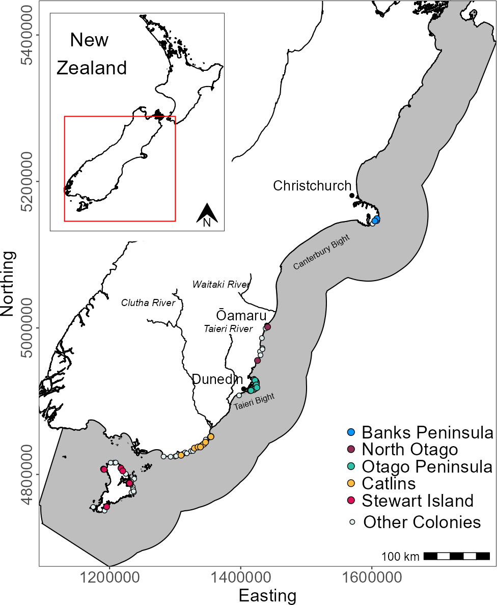
Figure 1 Distribution of breeding colonies across the South Island and Stewart Island, New Zealand and the GPS foraging trip data used in this study. Tracks and colonies are coloured by region. White circles denote colonies with at least one confirmed nest since 2003 but with no GPS tracking data. The grey area is the study extent.

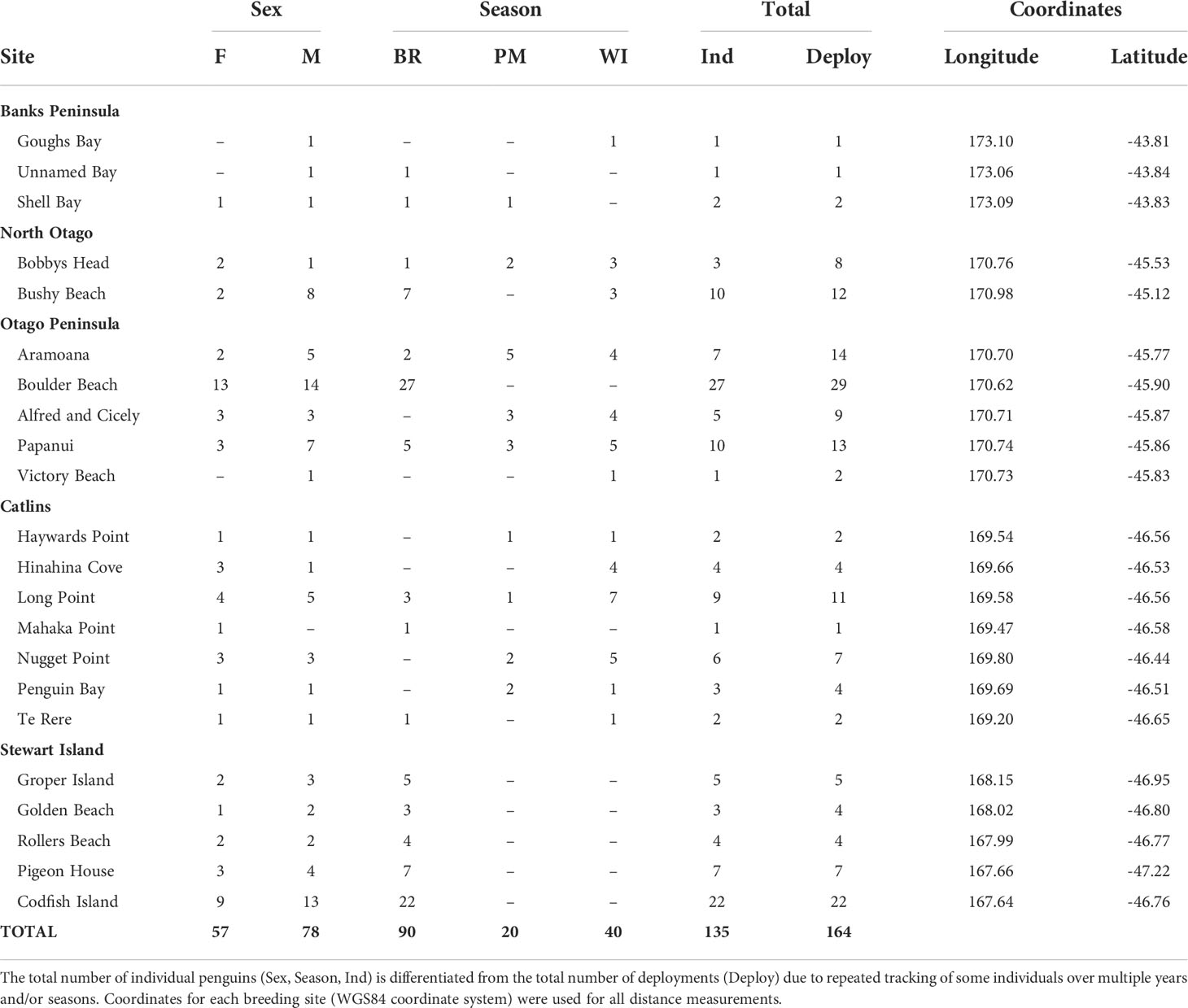
Table 1 Sample sizes of GPS-tracked, adult yellow-eyed penguins from each breeding colony and geographic region according to sex (female-F, male-M) and season (breeding-BR, premoult-PM, winter-WI).

For all device deployments, yellow-eyed penguins were intercepted at their nest or as they returned to their colonies after a foraging trip. Each penguin was weighed in a cloth bag to the nearest 50 g using a Pesola scale and head and foot measurements were taken using an osteometric board. Only penguins weighing more than 4.5 kg were fitted with a GPS dive logger. Using waterproof Tesa tape (No. 4651, Beiersdorf AG, Hamburg, Germany), the logger was attached to the dorsal feathers of the penguin’s lower back following the methodology of Wilson et al. (1997). For some longer deployments in 2019-2021, cable ties were inserted under the feathers and tightened around the device for additional attachment security. A rubber-based glue was spread over the top of the tape and cable ties (Mattern et al., 2007; Mattern et al., 2013). After a total handling time of < 20 minutes, the penguin was then released at the site of capture or within 1 m of the nest. The loggers were retrieved after 6-20 days in a manner that prevented plumage damage, and handling time was < 10 minutes.

All animal handling and data collection were permitted under several New Zealand Wildlife Act 1953 authorities (78325-FAU, 50925-FAU, SOUCO-45822 CR AP) and carried out in accordance with University of Otago’s Animal Ethics Authority AEC (AUP-19-92, 48/16, 32/03) and the New Zealand Department of Conservation Animal Ethics Committee (AEC336 and AEC389).

For data collected before 2016 (Mattern, 2006; Mattern et al., 2007; Mattern et al., 2013), GPS-TDlog devices were used (Earth and Ocean Technologies, Kiel, Germany; dimensions: L x W x H = 100 x 48 x 24 mm, mass: ca. 70 g). For data collected after 2016 (Elley et al., 2022; Young, 2022), Axy-Trek marine GPS-TDR loggers were used (Technosmart, Rome, Italy). The Axy-Trek loggers varied in size (L x W x H = 65 x 39 x 14 mm or 69 x 40 x 14 mm) and mass (46-59 g) depending on battery size. A 59 g GPS logger constitutes 1.1% of the body mass of a 5.5 kg yellow-eyed penguin (male mean breeding mass (Marchant and Higgins, 1990; Seddon et al., 2013). The frontal area of the loggers is less than 2.0% of a yellow-eyed penguin’s cross-sectional area (Mattern et al., 2007). The devices were streamlined and positioned low on the back to reduce drag (Bannasch et al., 1994; Ropert-Coudert et al., 2002). No effect of logger deployment on lifetime reproductive success (Stein et al., 2017), nest attendance, breeding success (Mattern et al., 2007), nor foraging capabilities (Mattern et al., 2018a) has been found in yellow-eyed penguins. The GPS loggers were programmed to record a geographical position at 60- or 90-second intervals during the day, with a 15-minute interval overnight from 23:00 – 06:00 to conserve battery while penguins are most likely on land. Pressure, depth, and temperature were recorded at a 1-second interval, and tri-axial accelerometer data were recorded at 25 Hz per second (Mattern, 2006; Mattern et al., 2007; Mattern et al., 2013).

Occurrence data

Data collected before 2016 were processed prior to this study with custom-written MATLAB code (v6.5, Mathworks, Inc., Natick, MA, USA; T. Mattern, unpub.). The supplied data included the GPS coordinates of each dive, timestamp, foraging trip number, maximum dive depth, and dive type (benthic or pelagic) classification. Refer to Mattern (2006) for a full methodology. We processed all data collected from 2016 onwards and conducted data analyses using custom-written scripts in R 4.0.3 (R Core Team, 2021), which are described henceforth along with the packages used for analyses. First, we removed any GPS points on land or indicating ground speed greater than or equal to 7.4 m/s (based on preliminary data exploration and expert knowledge) and any points derived from communications with fewer than three satellites to exclude inaccurate fixes (Recio et al., 2011). We differentiated individual foraging trips if the time interval between successive GPS points was greater than six hours. To account for irregular fix frequencies that occurred due to the limited surface time between dives, as well as possible differences in sample rate depending on the GPS settings, we linearly interpolated all GPS points per trip to 60-second intervals using the adehabitatLT package (v3.25) (Calenge, 2006). We omitted points that were interpolated between two GPS fixes if the temporal gap exceeded one hour.

We identified individual dive events from the depth, temperature, and accelerometer data recorded at 1-second intervals using the diveMove package (v1.5.2) (Luque, 2020). We zero-offset corrected each dive to account for potential drift in pressure sensors (Luque and Fried, 2011). For consistency of dive identification across multiple datasets, we accepted only dive events that exceeded 3 m (Mattern et al., 2013; Mattern et al., 2007). However, penguins from Groper Island, part of Stewart Island, performed an abundance of atypical, shallow foraging dives less than 1 m deep (verified via camera deployment, Mattern and Ellenberg, 2021), therefore dives exceeding 0.5 m were accepted for Groper Island penguins. To determine a geographic coordinate for each dive, we combined interpolated GPS points with dive data using the mean time between the beginning of descent and beginning of ascent and equivalent GPS timestamps, formatted using the lubridate package (v1.7) (Grolemund and Wickham, 2011).

We further sub-sampled one valid dive event per hour (first point/hour) for each foraging trip from 135 individuals tracked over 164 deployments to reduce temporal redundancy and spatial clustering (Hartel et al., 2020). We chose this method over other methods (e.g., distance sampling, random sampling), because it increased spatial and temporal independence while mitigating sampling differences (Boria et al., 2014). We split this final dataset into subsets according to subpopulation (Table 1). We used several R packages associated with tidyverse (Wickham et al., 2019), sp (v1.4-5) (Pebesma and Bivand, 2005; Bivand et al., 2013), and the raster package (v.3.3-13) (Hijmans, 2020) for general geographic data analyses.

Environmental data

We considered 19 high-resolution gridded environmental predictors (Table 2). Hydrographic features included long-term, annual mean concentrations of dissolved oxygen (sf_do), salinity (sf_salinity), nitrogen (sf_nitrogen), aragonite (sf_aragonite), and silicate (sf_silicate) at the seafloor, seafloor temperature (sf_temperature), and tidal current speed (currents), as well as long-term (2002-2018) mean, maximum, and minimum annual sea surface temperature (sst), chlorophyll a concentrations (chla), and turbidity (turb). Physical terrain features included seafloor sediment type percentages of mud, sand, gravel, carbonate (carbon) and bathymetry. Additionally, we considered several distance layers, as proxies for dispersal and geographic limitations. Using coordinates and nest counts queried from the Yellow-eyed Penguin Database (Department of Conservation, 2021), we calculated distance to (i) the nearest breeding colony with at least one nest since 2006 (distcolonyall) and to (ii) the nearest breeding colony where penguins were caught (distcolony) using the Euclidean Distance tool in ArcGIS Pro (v2.7.0) (ESRI Inc, 2019). This tool calculated the shortest Euclidean distance between the cell centres of an empty raster grid with a cell size of 500 m (i.e., fishnet raster) and the nearest feature of reference. We used the coastline of the South Island and Stewart Island, based on the Topo50 NZ Coastlines and Islands Polygons layer from the Land Information New Zealand Data Service (https://data.linz.govt.nz/) (LINZ, 2020) to delineate (iii) distance to land (distland) and the 500 m contour derived from the bathymetry layer to represent the (iv) distance to the continental shelf break (dist500m). We extracted the raster data to the extent of the empty fishnet raster that was used to derive the distance layers (Figure 1). During rescaling, we applied bilinear interpolation for layers that had a cell size greater than 500 m (e.g., sediment type) and took the mean value for layers that had a cell size less than 500 m (e.g., bathymetry). To compare distributions between subpopulations, we extracted and rasterised final predictors to 500 m resolution fishnet grids of five regional/subpopulation extents: (from north to south) Banks Peninsula, North Otago, Otago Peninsula, Catlins, and Stewart Island.

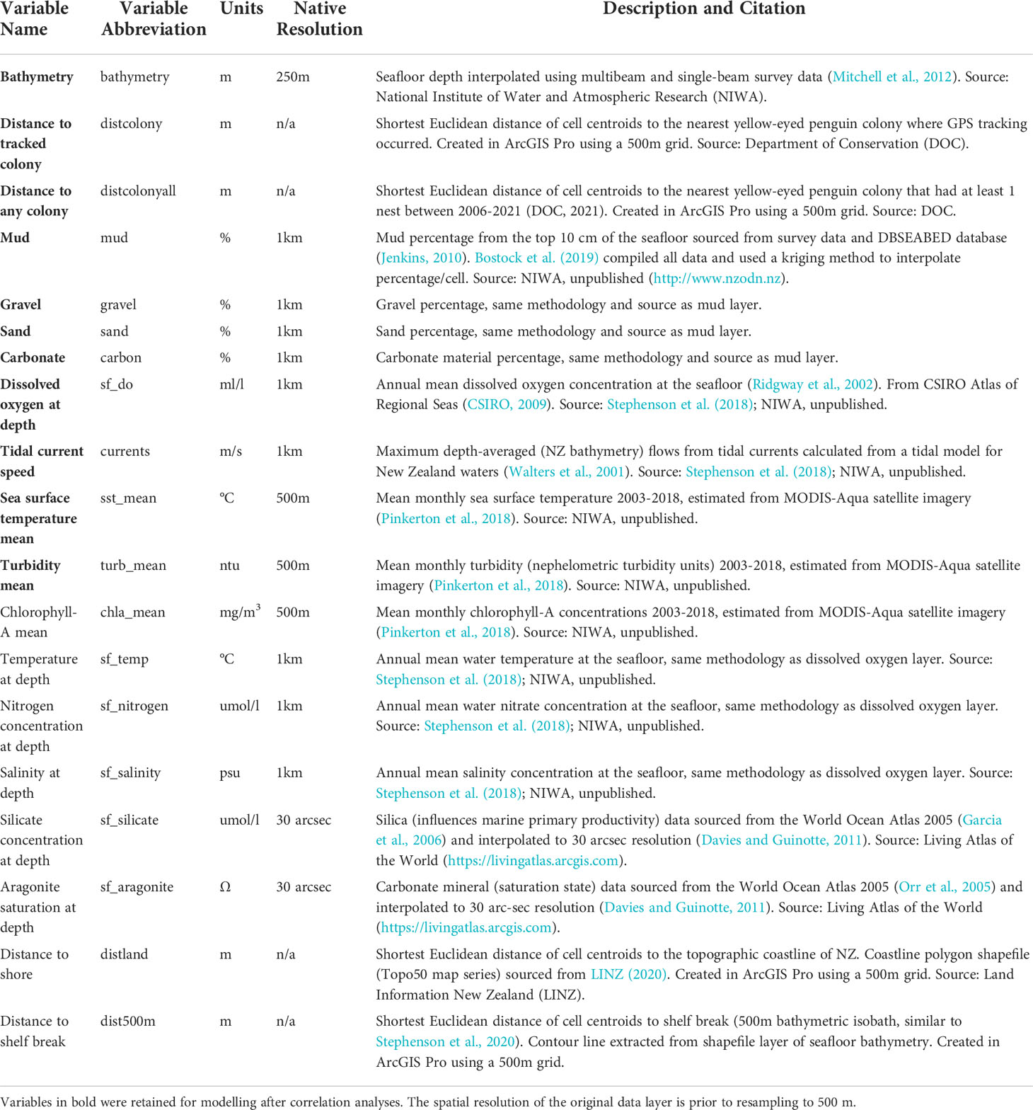
Table 2 Environmental predictor variables considered in Maxent species distribution models.

To avoid multicollinearity in the models, we removed collinear predictors with Spearman’s correlation coefficients > 0.7 or with variable inflation factors (VIF) > 10 (Dormann et al., 2013) using the usdm package (v1.1-18) (Naimi et al., 2014). See Supplementary Material Figure 1 for the correlation matrix created using the corrplot package (v0.84) (Wei and Simko, 2017). Some multicollinearity is acceptable in Maxent (Elith et al., 2011), so we subjectively retained several predictors that were hypothesised to be highly important for penguin distribution (e.g., bathymetry, seafloor sediment type). A final dataset of ten predictors were used for modelling (Figure 2): bathymetry, distcolony, current, mud, gravel, sand, carbon, sf_do, sst_mean, and turb_mean.

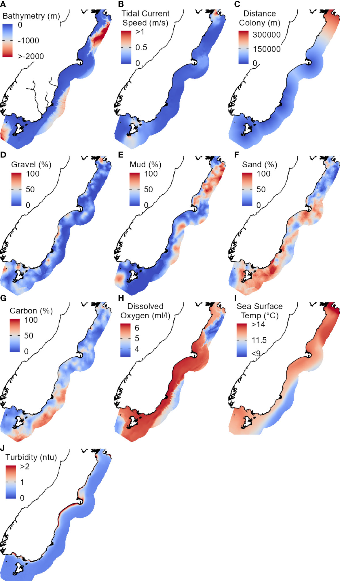
Figure 2 Environmental predictors (A-J) used in the final Maxent models. Study extent is a 75 km buffer off the east coast of the South Island, New Zealand. Abbreviations and units correspond to those in Table 2. Colour gradients range from high/maximum (red) to low/minimum (blue).

Model implementation

We used the machine-learning SDM method maximum entropy (Maxent v3.4.3) (Phillips et al., 2006) to model the marine habitat suitability for yellow-eyed penguins. Maxent is a frequently used, open-access, presence-only method appropriate for data obtained from high frequency GPS tracking (Phillips et al., 2006; Elith et al., 2011; Phillips et al., 2017) and has been shown to handle temporally or spatially correlated data (Afán et al., 2014; Ramírez et al., 2014; Boria et al., 2017; Recio et al., 2018; Hunter-Ayad et al., 2021). Maxent first assumes a uniform probability distribution for a species in space and then applies environmental variable constraints or features as functions to determine a potential probability distribution that best fits the data (Phillips et al., 2006). Maxent is similar to an inhomogeneous Poisson point process and gives an estimate of the intensity of occurrences at or near a grid cell centroid, which can be scaled to probability of presence using a complementary log-log link function (see Phillips et al., 2017). We fitted Maxent models using subsets of presence points for the South Island (SI) and the five regions representing each subpopulation. The SI model used the complete dataset of one foraging dive location per hour and 10,000 random background points (Barbet-Massin et al., 2012). For the subpopulation models, we used foraging locations from penguins originating from the specific region (Table 1), 5,000 random background points, and the environmental predictors for each regional extent.

Model optimisation and selection

We fitted 100 candidate models for the SI and each subpopulation, 600 models total, to determine optimal input parameters that are known to affect model complexity and prediction accuracy while accounting for the random partitioning of occurrence data (Merow et al., 2013; Radosavljevic and Anderson, 2014) using the ENMeval package (v0.3.1) (Muscarella et al., 2014). We selected the best combination of 20 regularisation multipliers (1-15 in 0.5 increments) and five feature class (L, LQ, LQH, LQHP, LQHPT, where L = linear, Q = quadratic, H = hinge, P = product, T = threshold functions; refer to Elith et al. (2011) for descriptions of each class) that minimised the sample size corrected Akaike Information Criterion (AICc), a frequently used evaluation measure of model fit and complexity (Warren and Seifert, 2011; Radosavljevic and Anderson, 2014). Regularisation multipliers and feature classes controls model complexity and fit, and tuning model parameters has been shown to improve Maxent model performance (Radosavljevic and Anderson, 2014).

Model evaluation

We employed k-fold cross-validation to evaluate the performance of all candidate models. We partitioned occurrence data into training and testing data using the “masked geographically structured” sampling method called “checkerboard2” using ENMeval to reduce inherent environmental biases and spatial autocorrelation (Muscarella et al., 2014; Radosavljevic and Anderson, 2014). To ensure the validation data were spatially independent, background points that occurred in the same geographic area as the testing data were not used for training.

We evaluated the final models using three statistics. The Area Under the Receiver Operating Characteristic Curve (AUC) statistic is a threshold-independent metric of model performance that quantifies the probability from 0.5 (no discrimination between presence and background point) to 1 (complete discrimination) that a random occurrence is ranked higher than a random background point (Phillips et al., 2006; Radosavljevic and Anderson, 2014). Two additional threshold-dependent metrics were calculated based on Omission Rates (OR) exceeding a certain threshold. The OR_MTP is a proportion of testing points that have a suitability value (relative occurrence rate) less than the lowest-ranking training point (minimum training presence); an OR_MTP of greater than 0 indicates model over-fitting. The OR₁₀ is a proportion of testing points that have a suitability value that is lower than the lowest-ranking training point excluding the lowest 10% of training points; an OR₁₀ greater than 10% indicates model over-fitting (Muscarella et al., 2014; Radosavljevic and Anderson, 2014).

Model predictions

We fitted the final SI and subpopulation models using the spatiotemporally filtered presence points and the optimal regularisation multiplier and feature class combination using the dismo package (v1.3-3) (Hijmans et al., 2020). For each model, Maxent predicted a probability of presence in geographic space using a cloglog output (Phillips et al., 2017; La Manna et al., 2020). To extrapolate the potential distribution of all yellow-eyed penguins breeding at any colony in the South Island, we exchanged the distance to a tracked colony (distcolony) layer with the distance to any colony layer (distcolonyall), keeping the geographic extent and all other predictors the same. To account for times outside of the breeding season, we fitted SI and subpopulation models with the same input setting and presences, but we excluded the distance to colony predictor (referred to as non-breeding or “nb” models), following a similar procedure to Mattern (2020). We used the same occurrence data to enable comparisons between distance and no distance model prediction maps, due to the lack of consistent seasonal differences in home range (Hickcox, data unpub.).

We converted the South Island model predictions into a binary environmental suitability map (Freeman and Moisen, 2008; Liu et al., 2016). This map was derived from a threshold method that assumed all areas with a predicted probability of presence equal to or greater than a certain threshold had environmental conditions suitable for occurrence (Ludynia et al., 2013; Hunter-Ayad et al., 2021). We chose a threshold that maximised the sum of sensitivity (true positive rate) and specificity (true negative rate), such that positive presences are just as likely to be incorrect as background points (Freeman and Moisen, 2008; Liu et al., 2016; Hunter-Ayad et al., 2021). The thresholds were 0.30 and 0.35 for the SI and SI (nb) models, respectively.

We plotted response curves for each environmental variable and ran a jack-knife analysis of variable importance for 2 final SI and 10 final subpopulation models. Values were normalised to percent contributions (PC) and were dependent upon the specific path used by Maxent. Permutation importance (PI) is determined by randomly permuting environmental variable values for the training points and normalising the resulting decrease in training AUC. We used ggplot2 (v3.3.3) (Wickham, 2016) and ggpubr (v0.4.0) (Kassambara, 2020) packages to create all figures. All maps are shown in the New Zealand Transverse Mercator 2000 projection.

Results

South Island models

For the SI model, the optimal input parameters that minimised the AICc were LQHP for the feature classes and 7.5 for the regularisation multiplier (see Supplementary Material Figures 2–6 for evaluation metric comparison plots for each SI and subpopulation model). Yellow-eyed penguins were distributed non-uniformly across their entire South Island marine range (Figure 3). The 135 individuals tracked over 164 deployments from 22 colonies (Table 1) foraged over the continental shelf, with the most suitable foraging habitat lying inshore (<20 km). The SI breeding season Maxent model indicated that distance to the nearest breeding colony was the most important predictor (Table 3) and had a negative relationship to habitat suitability (Figure 4J). Dissolved oxygen (DO) concentrations at depth had a permutation importance (PI) of 13.4% while all other variables were less than 2.5%.

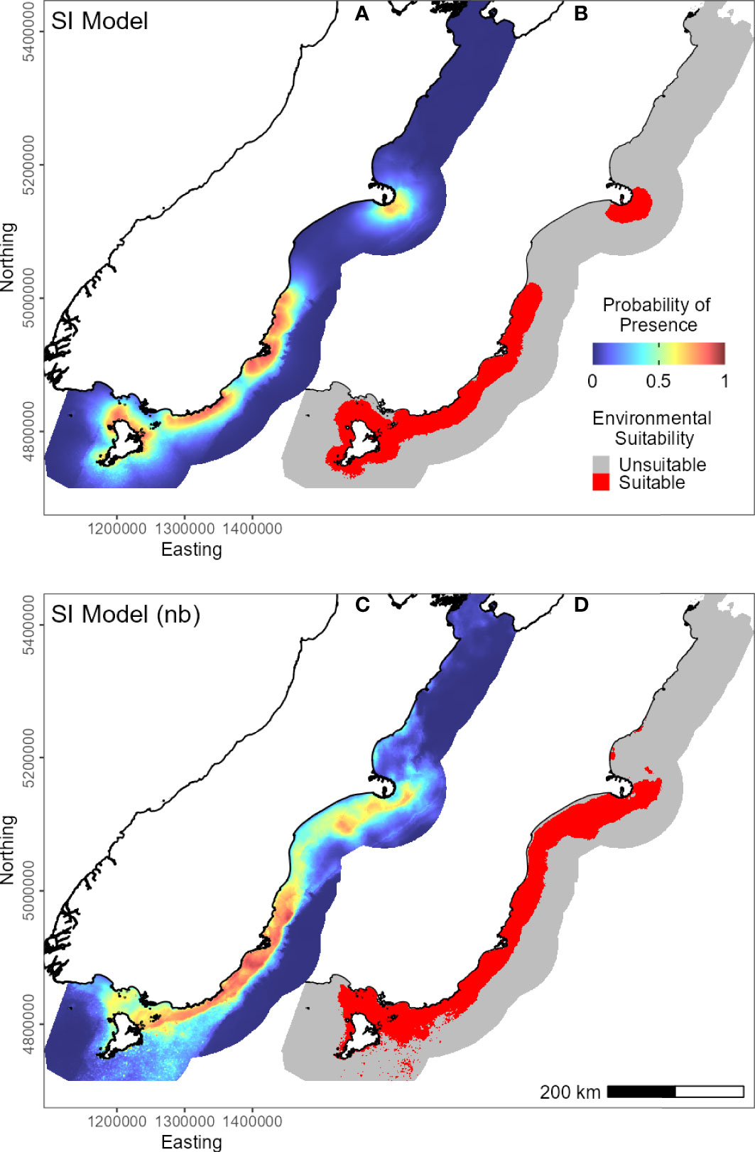
Figure 3 Predicted probability of presence (cloglog) of yellow-eyed penguins in New Zealand across their South Island marine range (A, C). Binary environmental suitability is shown on the right (B, D), with suitable habitat in red. The top two maps (A, B) include distance to the nearest colony as a predictor variable (SI model), while the bottom maps (C, D) do not include distance (SI model (nb)).

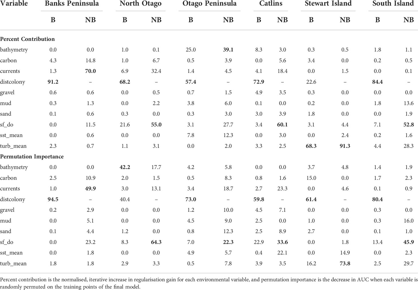
Table 3 Percent contribution and permutation importance (highest in bold) for the environmental variables used in the South Island and five regional Maxent models that include (B; breeding) and exclude (NB; non-breeding) distance to colony as a predictor.

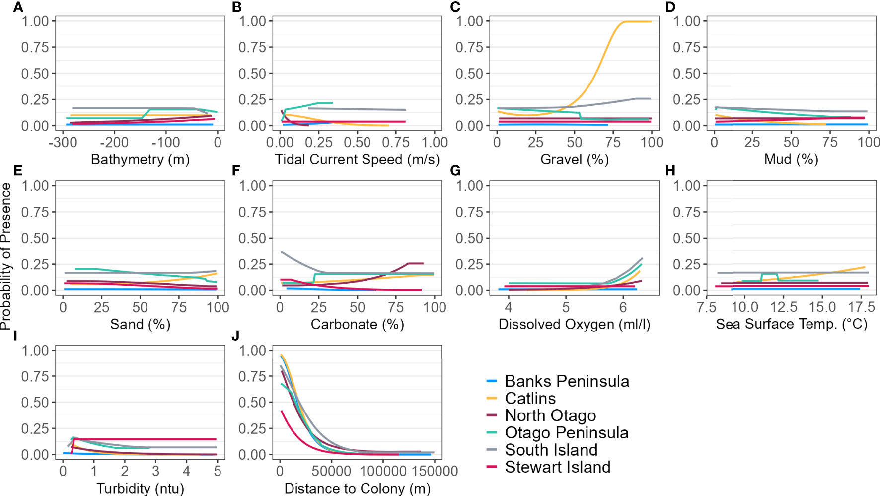
Figure 4 Response curves of each environmental predictor (A-J), including distance to colony, for each regional and South Island (SI) Maxent model predicting yellow-eyed penguin marine distribution.

The models predicted that yellow-eyed penguins can forage over a larger area outside of the breeding season when colony distance is not a limiting factor. Areas excluded from the breeding SI model had a higher predicted probability of presence (Figure 3B); for example, the Canterbury Bight (south of Banks Peninsula) and the Taieri Bight (north of the Taieri River mouth and south of the Otago Peninsula; Figure 1). The concentration of DO at the seafloor was the most important predictor (PI 45.9%; Table 3), confirmed by a positive relationship with probability of presence (Figure 5G). Mean turbidity had a PI of 29.7% followed by the percentage of seafloor mud with a PI of 16.0%. Both variables had a negative relationship with probability of presence (Figure 5). All other variables had a permutation importance of less than 2.5%.

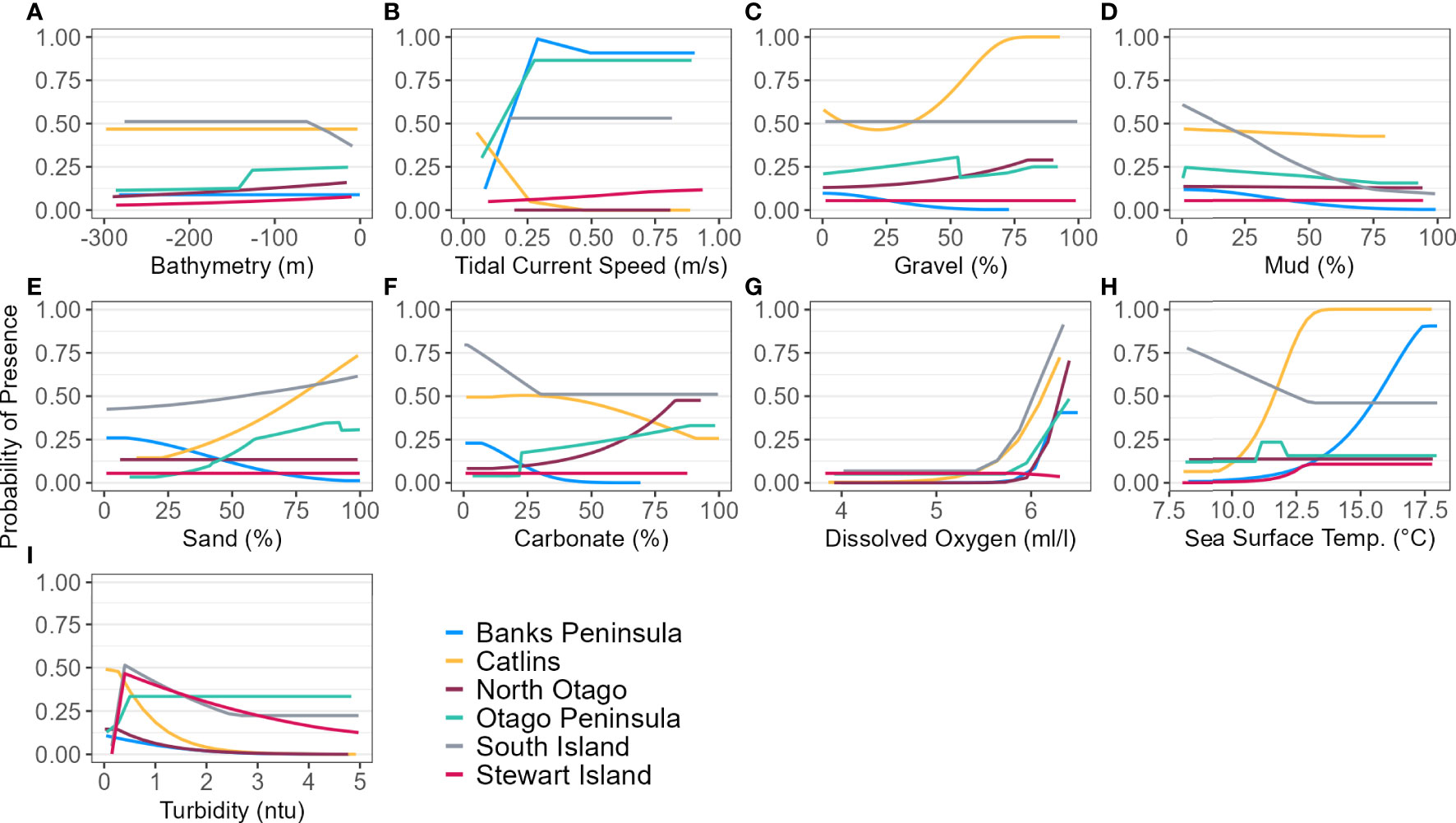
Figure 5 Response curves of each environmental predictor (A-I), excluding distance to colony, for each regional and South Island (SI) Maxent model predicting yellow-eyed penguin marine distribution.

Regional models

During model evaluation, the following feature classes and regularisation multipliers were found to minimise AICc in the subpopulation models: Banks Peninsula – LQ 4.0; North Otago – LQ 5.0; Otago Peninsula – LQHPT 7.0; Catlins – LQ 1; Stewart Island – LQH 12.5.

The marine distribution of penguins breeding on Banks Peninsula (n = 4 tracked penguins) extended east-southeast over the relatively wide continental shelf (Figure 6). Distance to the nearest colony was the most important variable in the model (PI 94.5%; Table 3), which resulted in a highly restricted, inshore distribution with probabilities greater than 0.5 ranging up to 30 km off the coast. Habitat suitability decreased north or south of Banks Peninsula (Figure 6). The Banks Peninsula (nb) model predicted a high probability of presence (≥ 0.75) where current speeds were greater than 0.25 m/s (PI 49.9%, Figure 5). The concentration of DO (PI 23.2%) was positively related to presence, while similar response curves with a negative relationship between all four sediment types suggests penguins search for prey over a more mixed seafloor substrate (Figures 5C–F) particularly as the percentage of sand or carbonate material increased (PI 4.4% and 10.9% respectively). All penguin dives occurred in areas with greater than 47.6% sand and less than 50% gravel, mud, or carbonate (Supplementary Material Table 1).

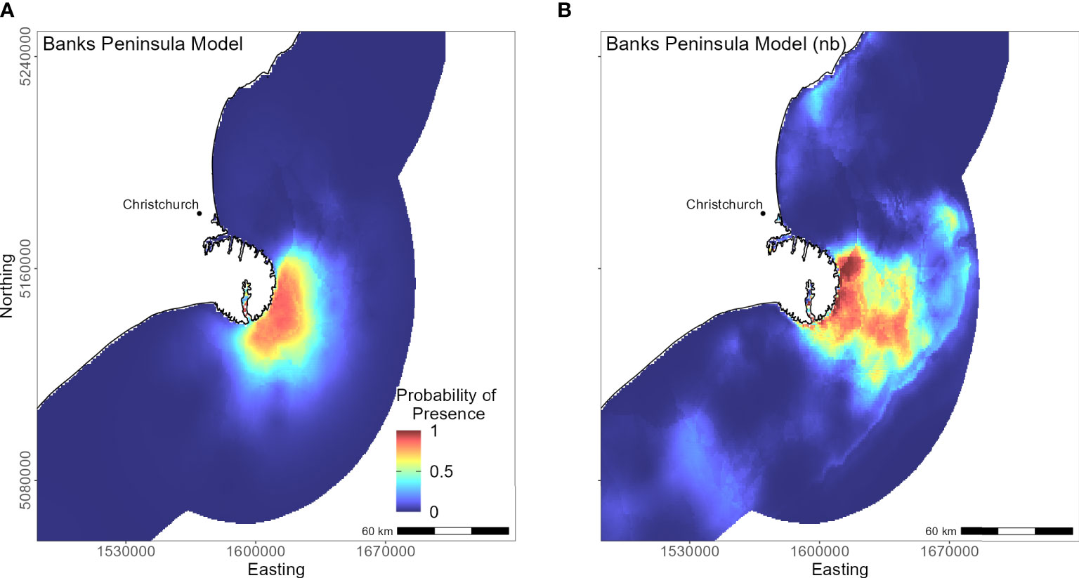
Figure 6 Distribution of suitable foraging habitat for yellow-eyed penguins breeding on Banks Peninsula. The left map (A) depicts the predicted probability of presence (cloglog) with distance to nearest colony included a predictor variable, while the right map (B) does not include distance to colony as a predictor (nb model).

Yellow-eyed penguins breeding in North Otago (n = 13) foraged east over a wide and shallow continental shelf (Figure 7). Bathymetry and distance to the nearest colony were the most important predictor variables (42.2% and 40.4%, respectively). Response curves showed a positive relationship between presence and bathymetry (Figure 4A), particularly at depths less than 150 m, and a negative relationship with distance to colony, which was similar to the Banks Peninsula response curve (Figure 4J). Without distance, the North Otago model (nb) predicted centres of suitable habitat further offshore in slightly deeper water, although the overall north-south distribution remained similar (Figure 7). The most important contributing variables when distance was not considered were DO concentration (PI 64.3%, Table 3), bathymetry (PI 17.7%), and current strength (PI 13.1%), with all other variables having an PI less than 3.5%. The mean depths at all dive locations in this region were the shallowest (34.8 ± 15.2 m) compared to other regions, with a maximum depth of only 88.8 m (Supplementary Material Table 1).

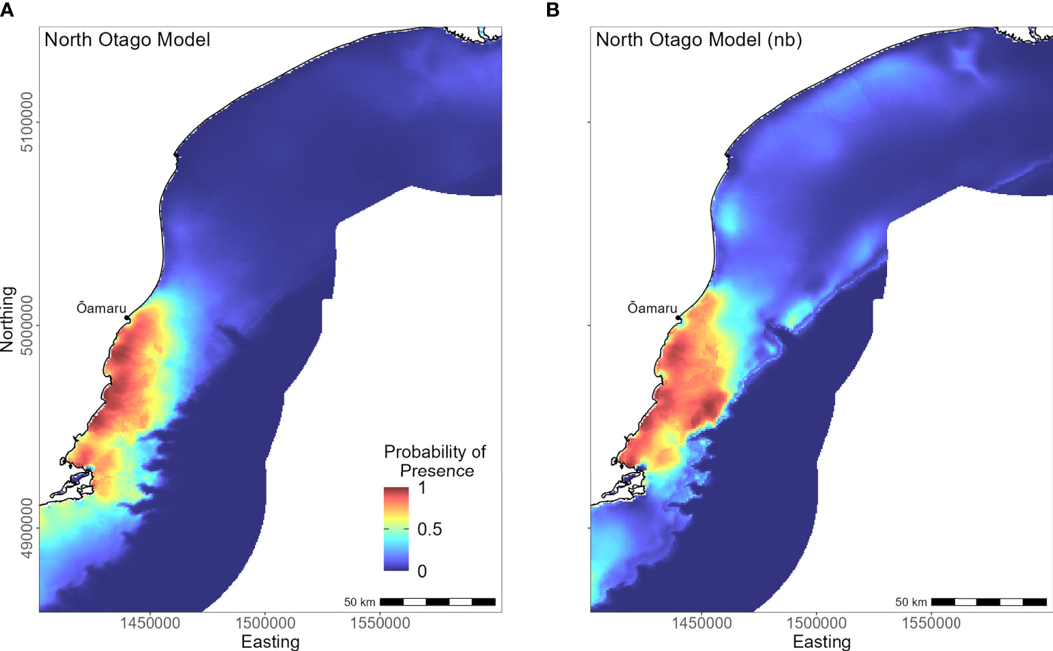
Figure 7 Distribution of suitable habitat for yellow-eyed penguins breeding on North Otago. The left map (A) depicts the predicted probability of presence (cloglog) with distance to nearest colony included a predictor variable, while the right map (B) does not include distance to colony as a predictor (nb model).

The Otago Peninsula Maxent model predicted that penguins were more likely (probability > 0.5) to forage up to approximately 35 km north, 20 km east, and 41 km south of the Otago Peninsula (n = 50; Figure 8). Off the Otago Peninsula, areas of suitable habitat were predicted for North Otago and Catlins penguins due to foraging overlap, a trend not seen in other regional models. Similar to the Banks Peninsula model, distance to the nearest colony was the primary predictor (PI 73.0%, Table 3), with PI of all others less than 7%. Compared to other regions, penguins from the Otago Peninsula foraged closest to their colonies, with a maximum distance to the nearest colony of 33 km (mean 9 ± 6 km; Supplementary Material Table 1). In non-breeding models, all remaining predictors had a permutation importance ranging from 22.3% (DO) to 5.7% (SST) (Table 3). Penguins were present in areas with more sand or carbonate sediment (Figure 5). About 25 km southwest of the Otago Peninsula, there was a distinct area directly off the coast at the mouth of the Taieri River which was predicted to be less suitable habitat for yellow-eyed penguins in both breeding and non-breeding models (Figure 8).

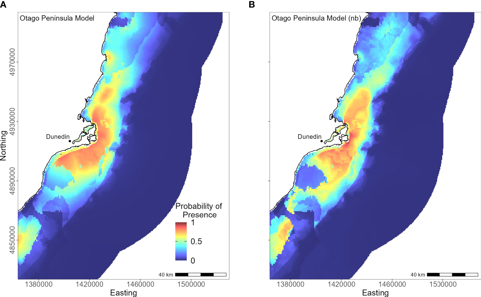
Figure 8 Distribution of suitable habitat for yellow-eyed penguins breeding on Otago Peninsula. The left map (A) depicts the predicted probability of presence (cloglog) with distance to nearest colony included a predictor variable, while the right map (B) does not include distance to colony as a predictor (nb model).

The continental shelf off the Catlins coast is narrow, and coastal waters are considerably deeper closer to shore. As a result, penguins (n = 37) foraged in deeper water (mean depth 77.7 ± 34.0 m; Supplementary Material Table 1) with key areas concentrated inshore (Figure 9); however, bathymetry was not a significant predictor variable. Rather, response curves showed similar relationships between environmental variables and the probability of presence as the South Island model, particularly for distance to the colony (PI 59.8%, Table 3) and DO (PI 22.9%). When distance was not considered, DO (PI 33.6%), mean current speed (PI 23.3%), and SST (PI 22.1%) were important to the model. Concentration of DO and SST had positive relationships with probability of presence (Figure 5), reflecting Banks Peninsula trends, although Catlins penguins were more likely to forage in cooler and deeper water (mean SST 12.0 ± 0.5°C; Supplementary Material Table 1). Catlins models predicted suitable habitat approximately 37 km from the Clutha River mouth (Figure 9), which is within the foraging range of Otago Peninsula penguins; however, the Otago Peninsula model predicted that Otago Peninsula penguins do not forage here.

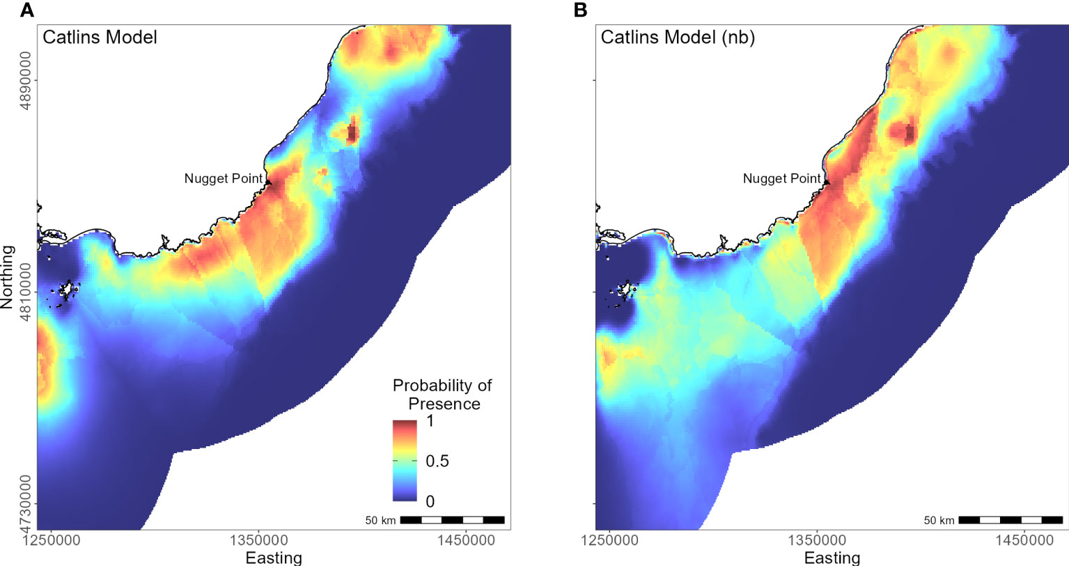
Figure 9 Distribution of suitable habitat for yellow-eyed penguins breeding in the Catlins. The left map (A) depicts the predicted probability of presence (cloglog) with distance to nearest colony included a predictor variable, while the right map (B) does not include distance to colony as a predictor (nb model).

Penguins from Stewart Island (n = 41) were predicted to forage within 3.75 km of Port Pegasus and within Paterson Inlet, but range further north of Codfish Island (Figure 10). Like the other regional models, distance to colony was the most important predictor (PI 61.4%; Table 3), followed by mean turbidity (PI 16.2%) and percent carbonate seafloor substrate (PI 15.0%). All other variables had a PI less than 4%, corroborated by flat response curves (Figure 4). In models not including distance, penguin distribution expanded further into Foveaux Strait (Figure 10). Mean turbidity had a large PI of 73.8%, indicating that Stewart Island penguins foraged in the least turbid waters compared to other regions (mean 0.5 ± 0.3 ntu; Supplementary Material Table 1). Response curves were similar to those for the SI model, except for turbidity which indicated a negative correlation with penguin presence when greater than 0.15 ntu (Figure 5).

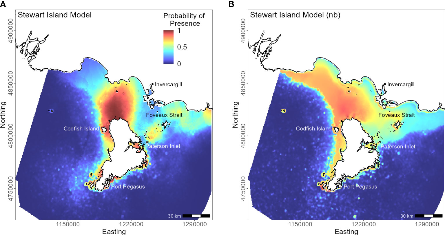
Figure 10 Distribution of suitable habitat for yellow-eyed penguins breeding on Stewart Island. The left map (A) depicts the predicted probability of presence (cloglog) with distance to nearest colony included a predictor variable, while the right map (B) does not include distance to colony as a predictor (nb model).

Discussion

This study is the first to compare the regional marine distributions of yellow-eyed penguins and to determine environmental predictor importance and general spatial patterns of habitat suitability across regions. All Maxent models confirmed that suitable foraging conditions for yellow-eyed penguins occur in the neritic zone over the continental shelf in waters less than 120-150 m deep. Similar to other central-place foraging seabirds including gentoo penguins (Pygoscelis papua; Harris et al., 2020), chinstrap penguins (P. antarcticus; Warwick-Evans et al., 2018), Scopoli’s shearwaters (Calonectris diomedea), and Cory’s shearwater (C. borealis; Afán et al., 2014), distance to the nearest colony was consistently the most important predictor of yellow-eyed penguin foraging distribution. Its high permutation importance in all models, ranging from 40.4% (North Otago) to 94.5% (Banks Peninsula), indicates that predicted use of suitable foraging areas is influenced more by colony proximity rather than by environmental conditions or prey availability. Accessibility of suitable foraging areas is likely a key determinant of breeding site selection, and thus the extent of their terrestrial distribution correlates to their foraging distribution as well.

Outside of the breeding season, penguins have no obligation to return regularly to their colony and are known to travel greater distances and for longer periods of time, which is supported by observed differences in dive behaviour and dispersal (Mattern, 2020; Young, 2022). When distance to the nearest colony was excluded, predicted suitable habitat expanded to include areas that post-breeding penguins could potential disperse to over longer foraging trips during the premoult and winter. Alternatively, these models could be interpreted as a theoretical, annual (breeding and non-breeding) distribution of habitat suitability for adult yellow-eyed penguins including non-breeders especially because these models do not predict suitable habitat that is unjustifiable based on their foraging behaviours (i.e., all areas are on the shelf in depths less than approximately 200 m deep). Although these models could also represent juvenile post-fledging dispersal, unique juvenile foraging behaviour by Young et al. (2022) suggests that separate models should be fitted to confirm habitat suitability.

Environmental predictors

Factors relating to prey availability were the most important determinants of yellow-eyed penguin foraging distribution and habitat selection. Other factors including bathymetry, SST, and seafloor sediment type had varying and marginal importance when predicting suitable foraging habitat. As visual predators, penguins rely on sight to identify, pursue, and capture prey (Boersma and Rebstock, 2009; Agnew, 2014; Mattern et al., 2018a). At the seafloor, light levels are diminished compared to higher in the water column, so penguins are only able to successfully capture benthic prey if visibility is adequate. As a result, areas of less turbid waters were predicted to be more suitable foraging habitat for yellow-eyed penguins. However, this study considered mean monthly estimates, so these models represent a mean tolerable range rather than a maximum/minimum range of turbidity levels. Like all other environmental factors, there is a finite range of acceptable turbidity that facilitates foraging success for yellow-eyed penguins (i.e., ‘Goldilocks’ zone; Da Silva et al., 2021), and while areas that exceed the mean turbidity range may be less suitable for foraging, they are not completely unsuitable; for instance, yellow-eyed penguins are known to forage in areas of poor visibility and high turbidity, particularly around Stewart Island where aquaculture farms operate.

Alternatively, increased turbidity could be an indication of nutrient mixing, sediment transport, or algal blooms due to increased water movement from coastal tides, currents, upwellings, or wind-driven waves (Bostock et al., 2019; Stevens et al., 2019). These conditions yield higher productivity through the water column, often mirrored at the seafloor because of downward nutrient fluxes and trophic cascades. However, when water becomes excessively turbid, light penetration, particularly to deeper depths, is impeded (Davies-Colley and Smith, 2001) which reduces photosynthesis at depth as well as the concentration of by-products such as DO (Mahaffey et al., 2020). Therefore, penguins foraging in less turbid waters would also be foraging in areas of high concentrations of DO. Similarly, DO had large permutation importance in most models (nb), and habitat suitability was greater in areas with a moderate DO concentration (5.9 – 6.3 ml/l). Consequently, there could be an underlying co-variance effect between these variables, although the saturation of oxygen in water is also dependent on temperature, water density, salinity, and other physical processes (Mahaffey et al., 2020). Since the indirect associations between yellow-eyed penguin habitat suitability and dynamic water properties including turbidity, DO, and temperature, are likely more related to prey availability, the potential global effects of climate change will have broad impacts not only on ocean productivity and nutrient cycling but also on prey and penguin occurrence and survival (Grémillet and Boulinier, 2009).

Based on previous studies of the dive behaviour of yellow-eyed penguins, which demonstrated a consistent and specialised benthic foraging strategy (e.g., Mattern et al., 2007), we hypothesised that seafloor depth would have a major influence on yellow-eyed penguin marine space use. Although their eastward dispersal from the coast is bounded by the continental shelf and the shelf break, which occurs at approximate depths of 125-150 m (Carter et al., 1985; Sutton, 2003; Gorman et al., 2013; Stevens et al., 2019), bathymetry had low importance in most of the models. This is also contrary to previous baseline spatial modelling showed its significance to regional habitat suitability (Mattern, 2020). Local bathymetry does, however, determine maximum dive depth which is variable across breeding sites. For example, penguins dive to maximum depths of 38.4 to 41.1 m off the coast of North Otago where mean seafloor depth is only -34.8 m (Mattern et al., 2007). In the Catlins where the seafloor is significantly deeper (mean depth -77.7 m), maximum dive depths of 156.2 m were achieved (Young, data unpubl.) . Additionally, dynamic predictors including DO, turbidity, and temperature are in some way affected by bathymetry (Cox et al., 2018). For instance, as depth increases, water temperature and DO concentration at the seafloor decrease. Seafloor depth and geomorphological features such as canyons or shelf breaks also affect horizontal and vertical water circulation and facilitate upwellings of nutrients (Cox et al., 2018), likely contributing to the patchy distribution of prey aggregations.

Because yellow-eyed penguins dive to all depths within their physiological capabilities, bathymetry is more of a threshold predictor. They forage at any depth less than a certain maximum depth. According to Wilson (1995), a c. 5.5 kg yellow-eyed penguin can theoretically reach a maximum dive depth of 146.6 m, so depths greater than this are less suitable for benthic foraging while any depth less than approximately 150 m could potentially be suitable habitat. This range denotes the continental shelf, so other continuous predictors which are also related to the continental shelf, such as DO and current strength, outweigh the importance of bathymetry in these models.

Compared to pelagic fish, the abundance of benthic fish is influenced more by bottom features (e.g., reefs, gravel outcrops) and substrate (Morrison et al., 2014 and references therein) than by dynamic processes such as the strength of currents or SST (Mattern et al., 2007). However, seafloor sediment type was not as important to yellow-eyed penguin foraging distribution as originally hypothesised, although fine-scale information may not be captured due to the scale used in our SDMs. Sediment type affected the Otago Peninsula penguin foraging range the most but had little impact on the North Otago and Stewart Island subpopulation models. If individuals exhibit foraging site fidelity and prey type preferences but variability across the population is high, the importance of seafloor sediment type would diminish as a predictor variable. For example, some penguins from Stewart Island might target mainly blue cod (Parapercis colias) on biogenic reefs, while other penguins preferentially prey on opalfish (Hemerocoetes sp.) in areas of gravel/coarse sand (Browne et al., 2011). Relatively few prey species comprise the majority of a yellow-eyed penguin’s diet (van Heezik, 1990), with a mean of 7.8 fish taxa identified from faecal samples by DNA metabarcoding (Young et al., 2020). These key species, however, are both pelagic and demersal, and the demersal prey can be found in diverse seafloor habitats; blue cod in disturbed, sandy or rocky benthic sediments (Morrison et al., 2014), red cod (Pseudophycis bachus) occur on sandy or muddy seafloors, and sprat (Sprattus sp.) can be found schooling midwater and occasionally at the seafloor (van Heezik, 1990). If seafloor sediment type is correlated with prey presence, then the weak relationship between yellow-eyed penguin presence and sediment type could be a result of the variation in diet. Areas of specific seafloor sediment or geomorphology such as reefs, rock outcrops, or trawl furrows might be cues for consistently productive prey patches, or be used as orientation or navigational aids to individual penguins (Mattern et al., 2013; van Eeden et al., 2016).

Along the east coast of the South Island, the northward flowing Southland Current determines local marine conditions. The Southland Current centres between -100 m and -40 m isobaths and is the global Subtropical Front convergence zone of inshore, warm, salty Subtropical Water and offshore, cold Subantarctic Water (Sutton, 2003; Stevens et al., 2019). Yellow-eyed penguins are associated with a productive frontal system, as are king penguins (Aptenodytes patagonicus; Bost et al., 2009), Magellanic penguins (Spheniscus magellanicus; Boersma and Rebstock, 2009), Fiordland penguins (Eudyptes pachyrhynchus; Mattern et al., 2018b), royal penguins (Eudyptes schlegeli; Hull et al., 1997), and most other penguin species. It is unknown whether this association is deliberate and penguins exploit productive prey patches aggregated by the front or simply that colonies are in proximity to the front. In conjunction with the continental shelf, however, the Southland Current is a boundary delineating selected foraging areas (Bost et al., 2009).

Conclusions

This study predicted the extent of suitable marine foraging habitat of yellow-eyed penguins in New Zealand for the first time. Regional variation was observed in habitat selection across their South Island extent, and dynamic variables related to prey availability were often the most important predictors in model predictions. Marine predators, including yellow-eyed penguins (Webster, 2018), are contending with anthropogenic exploitation of resources, marine habitat change and disturbance (Trathan et al., 2015), bycatch risks (Crawford et al., 2017), and climate change (Mattern et al., 2017). However, quantification of these threats and dynamic processes or temporal variability (e.g., after extreme weather events, El Niño Southern Oscillation) is not easily represented in species distribution models. For instance, since there is little evidence that foraging distances have changed significantly over time (Ellenberg and Mattern, 2012; Muller et al., 2021; Elley et al., 2022; Young, 2022), studies comparing diving behaviour (e.g., dive depth, bottom time) and diet over time may more clearly identify patterns of environmental change. Additionally, high quality environmental and commercial fisheries data are often unavailable or inaccessible, and the overall risk from fisheries interactions (e.g., overfishing, bycatch) remains largely unknown. By quantifying long-term marine habitat selection and space use, this study provides a more robust foundation for future studies of the spatial and temporal interactions between yellow-eyed penguins and their environment. These baseline models can be refined in future studies to investigate trends in distribution and environmental predictors over time. We can then predict possible shifts in the extent and location of foraging areas and where penguins might face increased or new anthropogenic threats, particularly if they move beyond targeted protected areas. The conservation of this endangered seabird depends on modelling studies such as these to identify critically important marine habitat and for identifying where future marine reserves should be located that account for the spatial variability in penguin foraging range.

Data availability statement

The majority of data analysed for this study are stored on Movebank (www.movebank.org) and can be made available by the authors upon reasonable request (Movebank study IDs: 1129010560, 7690187, 1348934678, 1594883659, 1507150714). R scripts can be found on Github (https://github.com/rphickcox/Yellow-eyedpenguinSDM_Hickcoxetal2022).

Ethics statement

The animal study was reviewed and approved by University of Otago’s Animal Ethics Authority and the New Zealand Department of Conservation Animal Ethics Committee.

Author contributions

RH, YH, and PS conceptualised the study. RH, TM, and MY performed field work, curated data, and acquired funding. RH, TM, and MR-R designed the methodology. RH conducted the analysis and wrote the original draft of the manuscript. TM, MR-R, YH, and PS supervised the project. All authors contributed to manuscript revision and approved the submitted version.

Funding

Funding was awarded to co-authors through the New Zealand Department of Conservation’s Conservation Services Programme (POP2016-05, POP2018-02, and POP2020-05). GPS tags were financed through grants from the Department of Conservation, Christchurch City Council, Yellow-eyed Penguin Trust, and Kelly Tarlton’s Marine Wildlife Trust. RH was funded by a University of Otago Postgraduate Scholarship.

Acknowledgments

We thank Te Rūnanga o Ngāi Tahu, each of the Papatipu Rūnaka, Roopū Kaitiaki, and the Whenua Hou Komiti for their consultation at the conceptualisation stage of the various tracking projects. Thank you to the many volunteers for field assistance, especially Thor Elley and Bryony Alden, Philippa Agnew, Julia Reid, Sarah Irvine, Ursula Ellenberg, Averil and Kevin Parthonnaud, Pōhatu Penguins/Plunge Ltd., and landowners for field site access. We are grateful for the support of the Department of Conservation, Christchurch City Council, Yellow-eyed Penguin Trust, and Kelly Tarlton’s Marine Wildlife Trust. Kind thanks to the Helps Pōhatu Conservation Trust for aiding in fieldwork travel and Dr. Matt Pinkerton (NIWA) and Dr. Fabrice Stephenson (NIWA) for supplying environmental data. Lastly, we thank two anonymous reviewers for their insightful comments. All work was permitted and complied with the current laws of New Zealand. This study comprises part of Rachel Hickcox’s PhD thesis, University of Otago.

Conflict of interest

The authors declare that the research was conducted in the absence of any commercial or financial relationships that could be construed as a potential conflict of interest.

Publisher’s note

All claims expressed in this article are solely those of the authors and do not necessarily represent those of their affiliated organizations, or those of the publisher, the editors and the reviewers. Any product that may be evaluated in this article, or claim that may be made by its manufacturer, is not guaranteed or endorsed by the publisher.

Supplementary material

The Supplementary Material for this article can be found online at: https://www.frontiersin.org/articles/10.3389/fmars.2022.967741/full#supplementary-material

References

Afán I., Navarro J., Cardador L., Ramírez F., Kato A., Rodríguez B., et al. (2014). Foraging movements and habitat niche of two closely related seabirds breeding in sympatry. Mar. Biol. 161, 657–668. doi: 10.1007/s00227-013-2368-4
Agnew P. (2014). Demographic parameters, foraging and responses to environmental variation of little penguins (Eudyptula minor). [Thesis]. Dunedin (NZ): University of Otago.
Bannasch R., Wilson R. P., Culik B. (1994). Hydrodynamic aspects of design and attachment of a back-mounted device in penguins. J. Exp. Biol. 194, 83–96.
Barbet-Massin M., Jiguet F., Albert C. H., Thuiller W. (2012). Selecting pseudo-absences for species distribution models: how, where and how many? Methods Ecol. Evol. 3, 327–338. doi: 10.1111/j.2041-210X.2011.00172.x
BirdLife International. (2020). Megadyptes antipodes. IUCN Red List Threatened Species 2020. doi: 10.2305/IUCN.UK.2020-3.RLTS.T22697800A182703046.en
Bivand R., Pebesma E., Gomez-Rubio V. (2013). Applied spatial data analysis with {R}. 2nd ed. (NY: Springer).
Boersma P. D., Rebstock G. A. (2009). Foraging distance affects reproductive success in magellanic penguins. Mar. Ecol. Prog. Ser. 375, 263–275. doi: 10.3354/meps07753
Boria R. A., Olson L. E., Goodman S. M., Anderson R. P. (2014). Spatial filtering to reduce sampling bias can improve the performance of ecological niche models. Ecol. Modell. 275, 73–77. doi: 10.1016/j.ecolmodel.2013.12.012
Boria R. A., Olson L. E., Goodman S. M., Anderson R. P. (2017). A single-algorithm ensemble approach to estimating suitability and uncertainty: cross-time projections for four Malagasy tenrecs. Divers. Distrib. 23, 196–208. doi: 10.1111/ddi.12510
Bost C.-A., Cotté C., Bailleul F., Cherel Y., Charrassin J.-B., Guinet C., et al. (2009). The importance of oceanographic fronts to marine birds and mammals of the southern oceans. J. Mar. Syst. 78, 363–376. doi: 10.1016/j.jmarsys.2008.11.022
Bostock H., Jenkins C., Mackay K., Carter L., Nodder S., Orpin A., et al. (2019). Distribution of surficial sediments in the ocean around New Zealand/Aotearoa. Part B: continental shelf. New Zeal. J. Geol. Geophys. 62, 24–45. doi: 10.1080/00288306.2018.1523199
Browne T., Lalas C., Mattern T., van Heezik Y. (2011). Chick starvation in yellow-eyed penguins: Evidence for poor diet quality and selective provisioning of chicks from conventional diet analysis and stable isotopes. Austral Ecol. 36, 99–108. doi: 10.1111/j.1442-9993.2010.02125.x
Calenge C. (2006). The package “adehabitat” for the r software: A tool for the analysis of space and habitat use by animals. Ecol. Modell. 197, 516–519. doi: 10.1016/j.ecolmodel.2006.03.017
Carter R., Carter L., Williams J., Landis C. (1985). Modern and relict sedimentation on the south Otago continental shelf, New Zealand. New Zeal. Oceanogr. Inst. Mem. 93, 1–43.
Chilvers B. L., Dobbins M., Edmonds H. (2014). Diving behaviour of yellow-eyed penguins, port Pegasus/Pikihatiti, Stewart Island/Rakiura, New Zealand. New Zeal. J. Zool 41, 161–170. doi: 10.1080/03014223.2014.908931
Cox S. L., Embling C. B., Hosegood P. J., Votier S. C., Ingram S. N. (2018). Oceanographic drivers of marine mammal and seabird habitat-use across shelf-seas: A guide to key features and recommendations for future research and conservation management. Estuar. Coast. Shelf Sci. 212, 294–310. doi: 10.1016/j.ecss.2018.06.022
Crawford R., Ellenberg U., Frere E., Hagen C., Baird K., Brewin P., et al. (2017). Tangled and drowned: a global review of penguin bycatch in fisheries. Endanger. Species Res. 34, 373–396. doi: 10.3354/esr00869
CSIRO (2009) Commonwealth scientific and industrial research organisation (CSIRO) atlas of regional seas. Available at: www.cmar.csiro.au/cars (Accessed December 16, 2020).
Da Silva C., Kerwath S. E., Winker H., Lamberth S. J., Attwood C. G., Wilke C. G., et al. (2021). Testing the waters to find the “goldilocks” zone: Fine-scale movement of mustelus mustelus in relation to environmental cues. Mar. Freshw. Res. 73, 110–124. doi: 10.1071/MF20369
Davies-Colley R. J., Smith D. G. (2001). Turbidity, suspended sediment and water clarity: a review. J. Am. Water Resour. Assoc. 37, 1085–1101.
Davies A. J., Guinotte J. M. (2011). Global habitat suitability for framework-forming cold-water corals. PloS One 6, e18483. doi: 10.1371/journal.pone.0018483
Department of Conservation (2021). Yellow-eyed penguin database. Department of Conservation. Dunedin, NZ: Department of Conservation.
Dormann C. F., Elith J., Bacher S., Buchmann C., Carl G., Carré G., et al. (2013). Collinearity: a review of methods to deal with it and a simulation study evaluating their performance. Ecography (Cop.). 36, 27–46. doi: 10.1111/j.1600-0587.2012.07348.x
Elith J., Phillips S. J., Hastie T., Dudík M., Chee Y. E., Yates C. J. (2011). A statistical explanation of MaxEnt for ecologists. Divers. Distrib. 17, 43–57. doi: 10.1111/j.1472-4642.2010.00725.x
Ellenberg U., Mattern T.. (2012). Yellow-eyed penguin - Review of population information. Dunedin, NZ: Department of Conservation.
Elley T., Mattern T., Ellenberg U., Young M. J., Hickcox R. P., van Heezik Y., et al. (2022). Consistent site-specific foraging behaviours of yellow-eyed penguins/hoiho breeding on Stewart island, New Zealand. Biol. 11, 844. doi: 10.3390/biology11060844
Franklin J., Miller J. A. (2009). Mapping species distributions: Spatial inference and prediction (Cambridge, UK: Cambridge University Press).
Freeman E. A., Moisen G. G. (2008). A comparison of the performance of threshold criteria for binary classification in terms of predicted prevalence and kappa. Ecol. Modell. 217, 48–58. doi: 10.1016/j.ecolmodel.2008.05.015
Garcia H. E., Locarnini R. A., Boyer T. P., Antonov J. I. (2006). ““World ocean atlas 2005, volume 4: Nutrients (phosphate, nitrate, silicate),”,” in NOAA Atlas NESDIS. Ed. Levitus S. (Washington, DC: U.S. Government Printing Office), 1–396.
Gorman A., Hill M., Orpin A., Koons P., Norris R., Landis C., et al. (2013). Quaternary shelf structures SE of the South Island, imaged by high-resolution seismic profiling. New Zeal. J. Geol. Geophys. 56, 68–82. doi: 10.1080/00288306.2013
Grémillet D., Boulinier T. (2009). Spatial ecology and conservation of seabirds facing global climate change: a review. Mar. Ecol. Prog. Ser. 391, 121–137. doi: 10.3354/meps08212
Grolemund G., Wickham H. (2011). Dates and times made easy with lubridate. J. Stat. Software 40, 1–25. doi: 10.18637/jss.v040.i03
Harris S., Scioscia G., Pütz K., Mattern T., Raya Rey A. (2020). Niche partitioning between coexisting gentoo Pygoscelis papua and magellanic penguins Spheniscus magellanicus at Martillo Island, Argentina. Mar. Biol. 167, 1–10. doi: 10.1007/s00227-020-03722-w
Hartel E. F., Noke Durden W., O’Corry-Crowe G. (2020). Testing satellite telemetry within narrow ecosystems: Nocturnal movements and habitat use of bottlenose dolphins within a convoluted estuarine system. Anim. Biotelemetry 8, 1–16. doi: 10.1186/s40317-020-00200-4
Hijmans R. J. (2020) Raster: geographic data analysis and modeling. Available at: https://cran.r-project.org/package=raster.
Hijmans R. J., Phillips S. J., Leathwick J., Elith J. (2020) Dismo: Species distribution modeling. Available at: https://cran.r-project.org/package=dismo.
Hopkins J., Shaw A. G. P., Challenor P. (2010). The Southland Front, New Zealand: Variability and ENSO correlations. Cont. Shelf Res. 30, 1535–1548. doi: 10.1016/j.csr.2010.05.016
Hull C. L., Hindell M. A., Michael K. (1997). Foraging zones of royal penguins during the breeding season, and their association with oceanographic features. Mar. Ecol. Prog. Ser. 153, 217–228. doi: 10.3354/meps153217
Hunter-Ayad J., Jarvie S., Greaves G., Digby A., Ohlemüller R., Recio M. R., et al. (2021). Novel conditions in conservation translocations: A conservative-extrapolative strategic framework. Front. Conserv. Sci. 2. doi: 10.3389/fcosc.2021.691714
Jenkins C. (2010) dbSEABED: Seafloor substrates. Available at: http://csdms.colorado.edu/wiki/Data:DBSEABED.
Kassambara A. (2020) Ggpubr: “ggplot2” based publication ready plots. Available at: https://cran.r-project.org/package=ggpubr.
Kowalczyk N. D., Reina R. D., Preston T. J., Chiaradia A. (2015). Environmental variability drives shifts in the foraging behaviour and reproductive success of an inshore seabird. Oecologia 178, 967–979. doi: 10.1007/s00442-015-3294-6
La Manna G., Ronchetti F., Sarà G., Ruiu A., Ceccherelli G. (2020). Common bottlenose dolphin protection and sustainable boating: Species distribution modeling for effective coastal planning. Front. Mar. Sci. 7. doi: 10.3389/fmars.2020.542648
LINZ (2020) NZ Coastlines and islands polygons (Topo 1:50k). Available at: https://data.linz.govt.nz/layer/51153-nz-coastlines-and-islands-polygons-topo-150k/.
Liu C., Newell G., White M. (2016). On the selection of thresholds for predicting species occurrence with presence-only data. Ecol. Evol. 6, 337–348. doi: 10.1002/ece3.1878
Ludynia K., Dehnhard N., Poisbleau M., Demongin L., Masello J. F., Voigt C. C., et al. (2013). Sexual segregation in rockhopper penguins during incubation. Anim. Behav. 85, 255–267. doi: 10.1016/j.anbehav.2012.11.001
Luque S. P. (2020) diveMove: Dive analysis and calibration. Available at: https://cran.r-project.org/package=diveMove.
Luque S. P., Fried R. (2011). Recursive filtering for zero offset correction of diving depth time series with GNU r package diveMove. PloS One 6, e15850. doi: 10.1371/journal.pone.0015850
Mahaffey C., Palmer M., Greenwood N., Sharples J. (2020). Impacts of climate change on dissolved oxygen concentration relevant to the coastal and marine environment around the UK. MCCIP Sci. Rev. 2020, 31–53. doi: 10.14465/2020.arc02.oxy
Marchant S., Higgins P. J. (1990). Handbook of Australian, New Zealand, and Antarctic birds. Melbourne: Oxford University Press.
Masello J. F., Mundry R., Poisbleau M., Demongin L., Voigt C. C., Wikelski M., et al. (2010). Diving seabirds share foraging space and time within and among species. Ecosphere 1, 1–28. doi: 10.1890/ES10-00103.1
Mattern T. (2006). Marine ecology of offshore and inshore foraging penguins: the snares penguin Eudyptes Robustus and yellow-eyed penguin Megadyptes Antipodes. [Thesis]. Dunedin (NZ): University of Otago.
Mattern T. (2020). Modelling marine habitat utilisation by yellow-eyed penguins along their mainland distribution: baseline information. Wellington, NZ: Fisheries New Zealand.
Mattern T., Ellenberg U. (2018). Yellow-eyed penguin diet and indirect effects on prey composition. Report for POP2011-08. (Dunedin, NZ: Department of Conservation). doi: 10.13140/RG.2.2.23828.81284
Mattern T., Ellenberg U. (2021). Report for POP2020-05. Q2 - quarterly progress report for the period 21 Dec 2020 –20 Mar 2021. doi: 10.6084/m9.figshare.14374385.v1
Mattern T., Ellenberg U., Houston D. M., Davis L. S. (2007). Consistent foraging routes and benthic foraging behaviour in yellow-eyed penguins. Mar. Ecol. Prog. Ser. 343, 295–306. doi: 10.3354/meps06954
Mattern T., Ellenberg U., Houston D. M., Lamare M., Davis L. S., van Heezik Y., et al. (2013). Straight line foraging in yellow-eyed penguins: New insights into cascading fisheries effects and orientation capabilities of marine predators. PLoS One 8, e84381. doi: 10.1371/journal.pone.0084381
Mattern T., Ellenberg U. (2018a). Report No.: DOC-POP2011-08. Yellow-eyed penguin diet and indirect effects on prey composition. Available at: https://www.researchgate.net/publication/325158074_Yellow-eyed_penguin_diet_and_indirect_effects_affecting_prey_composition_-_Collation_of_biological_information
Mattern T., Meyer S., Ellenberg U., Houston D. M., Darby J. T., Young M. J., et al. (2017). Quantifying climate change impacts emphasises the importance of managing regional threats in the endangered yellow-eyed penguin. PeerJ 5, e3272. doi: 10.7717/peerj.3272
Mattern T., Pütz K., García-Borboroglu P., Ellenberg U., Houston D. M., Long R., et al. (2018b). Marathon penguins – reasons and consequences of long-range dispersal in fiordland penguins/tawaki during the pre-moult period. PloS One 13, e0198688. doi: 10.1371/journal.pone.0198688
Merow C., Smith M. J., Silander J. A. (2013). A practical guide to MaxEnt for modeling species’ distributions: what it does, and why inputs and settings matter. Ecography (Cop.). 36, 1058–1069. doi: 10.1111/j.1600-0587.2013.07872.x
Mitchell J., Mackay K., Neil H., Mackay E., Pallentin A., Notman P. (2012). “Undersea New Zealand, 1:5,000,000,” in NIWA chart, misc. ser. Auckland, NZ: NIWA.
Moore P. J. (1999). Foraging range of the yellow-eyed penguin Megadyptes antipodes. Mar. Ornithol. 27, 56–58.
Moore P. J., Wakelin M., Douglas M. E., McKinlay B., Nelson D., Murphy B. (1995). Yellow-eyed penguin foraging study, south-eastern New Zealand 1991–1993. (Wellington, NZ: Department of Conservation).
Morrison M., Jones E., Parsons D., Grant C. (2014). Habitats and areas of particular significance for coastal finfish fisheries management in New Zealand: A review of concepts and current knowledge, and suggestions for future research (Wellington, NZ: Ministry for Primary Industries).
Muller C. G., Chilvers B. L., French R. K., Battley P. F. (2020). Diving plasticity in the ancestral range of the yellow-eyed penguin Megadyptes antipodes, an endangered marine predator. Mar. Ecol. Prog. Ser. 648, 191–205. doi: 10.3354/meps13415
Muller C. G., Chilvers B. L., Chiaradia A., French R. K., Kato A., Ropert-Coudert Y., et al (2021). Foraging areas and plasticity of yellow-eyed penguins Megadyptes antipodes in their Subantarctic range. Mar. Ecol. Prog. Ser. 679, 149–162. doi: 10.3354/meps13911
Muscarella R., Galante P. J., Soley-Guardia M., Boria R. A., Kass J. M., Uriarte M., et al. (2014). ENMeval: An r package for conducting spatially independent evaluations and estimating optimal model complexity for maxent ecological niche models. Methods Ecol. Evol. 5, 1198–1205. doi: 10.1111/2041-210x.12261
Naimi B., Hamm N. A., Groen T. A., Skidmore A. K., Toxopeus A. G. (2014). Where is positional uncertainty a problem for species distribution modelling? Ecography (Cop.). 37, 191–203. doi: 10.1111/j.1600-0587.2013.00205.x
Orr J. C., Fabry V. J., Aumont O., Bopp L., Doney S. C., Feely R. A., et al. (2005). Anthropogenic ocean acidification over the twenty-first century and its impact on calcifying organisms. Nature 437, 681–686. doi: 10.1038/nature04095
Peacock L., Paulin M., Darby J. T. (2000). Investigations into climate influence on population dynamics of yellow-eyed penguins Megadyptes antipodes. New Zeal. J. Zool. 27, 317–325. doi: 10.1080/03014223.2000.9518241
Phillips S. J., Anderson R. P., Dudík M., Schapire R. E., Blair M. E. (2017). Opening the black box: an open-source release of maxent. Ecography (Cop.). 40, 887–893. doi: 10.1111/ecog.03049
Phillips S. J., Anderson R. P., Schapire R. E. (2006). Maximum entropy modeling of species geographic distributions. Ecol. Modell. 190, 231–259. doi: 10.1016/j.ecolmodel.2005.03.026
Pinkerton M., Gall M., Wood S., Zeldis J. (2018). Measuring the effects of bivalve mariculture on water quality in northern New Zealand using 15 years of MODIS-Aqua satellite observations. Aquac. Environ. Interact. 10, 529–545. doi: 10.3354/AEI00288
Radosavljevic A., Anderson R. P. (2014). Making better maxent models of species distributions: Complexity, overfitting and evaluation. J. Biogeogr. 41, 629–643. doi: 10.1111/jbi.12227
Ramírez F., Afán I., Hobson K. A., Bertellotti M., Blanco G., Forero M. G. (2014). Natural and anthropogenic factors affecting the feeding ecology of a top marine predator, the magellanic penguin. Ecosphere 5 (4), 1–21. doi: 10.1890/ES13-00297.1
R Core Team (2021) R: A language and environment for statistical computing. Available at: https://www.r-project.org.
Recio M. R., Mathieu R., Denys P., Sirguey P., Seddon P. J. (2011). Lightweight GPS-tags, one giant leap for wildlife tracking? An assessment approach. PloS One 6, e28225. doi: 10.1371/journal.pone.0028225
Recio M. R., Zimmermann B., Wikenros C., Zetterberg A., Wabakken P., Sand H. (2018). Integrated spatially-explicit models predict pervasive risks to recolonizing wolves in Scandinavia from human-driven mortality. Biol. Conserv. 226, 111–119. doi: 10.1016/j.biocon.2018.07.025
Ridgway K. R., Dunn J. R., Wilkin J. L. (2002). Ocean interpolation by four-dimensional weighted least squares–application to the waters around Australasia. J. Atmos. Ocean. Technol. 19, 1357–1375. doi: 10.1175/1520-0426(2002)019<1357:OIBFDW>2.0.CO;2
Ropert-Coudert Y., Chiaradia A., Ainley D. G., Barbosa A., Boersma P. D., Brasso R., et al. (2019). Happy feet in a hostile world? the future of penguins depends on proactive management of current and expected threats. Front. Mar. Sci. 6. doi: 10.3389/FMARS.2019.00248
Ropert-Coudert Y., Kato A., Bost C.-A., Rodary D., Sato K., Le Maho Y., et al. (2002). Do adélie penguins modify their foraging behaviour in pursuit of different prey? Mar. Biol. 140, 647–652. doi: 10.1007/s00227-001-0719-z
Seddon P. J., Ellenberg U., Van Heezik Y. (2013). “Yellow-eyed penguin,”” in Penguins: Natural History and Conservation. Eds. García-Borboroglu P., Boersma P. D. (Seattle, WA: University of Washington Press), 91–113.
Stein A. M., Young M. J., Seddon P. J., Darby J. T., van Heezik Y. (2017). Investigator disturbance does not reduce annual breeding success or lifetime reproductive success in a vulnerable long-lived species, the yellow-eyed penguin. Biol. Conserv. 207, 80–89. doi: 10.1016/J.BIOCON.2017.01.013
Stephenson F., Goetz K., Sharp B. R., Mouton T. L., Beets F. L., Roberts J., et al. (2020). Modelling the spatial distribution of cetaceans in New Zealand waters. Divers. Distrib. 26, 495–516. doi: 10.1111/ddi.13035
Stephenson F., Leathwick J. R., Geange S. W., Bulmer R. H., Hewitt J. E., Anderson O. F., et al. (2018). Using gradient forests to summarize patterns in species turnover across large spatial scales and inform conservation planning. Divers. Distrib. 24, 1641–1656. doi: 10.1111/ddi.12787
Stevens C. L., O’Callaghan J. M., Chiswell S. M., Hadfield M. G. (2019). Physical oceanography of New Zealand/Aotearoa shelf seas – a review. New Zeal. J. Mar. Freshw. Res. 55, 6–45. doi: 10.1080/00288330.2019.1588746
Sutton P. J. (2003). The southland current: A subantarctic current. New Zeal. J. Mar. Freshw. Res. 37, 645–652. doi: 10.1080/00288330.2003.9517195
Trathan P. N., García-Borboroglu P., Boersma P. D., Bost C.-A., Crawford R. J., Crossin G. T., et al. (2015). Pollution, habitat loss, fishing, and climate change as critical threats to penguins. Conserv. Biol. 29, 31–41. doi: 10.1111/cobi.12349
van Eeden R., Reid T., Ryan P. G., Pichegru L. (2016). Fine-scale foraging cues for African penguins in a highly variable marine environment. Mar. Ecol. Prog. Ser. 543, 257–271. doi: 10.3354/meps11557
van Heezik Y. (1990). Seasonal, geographical, and age-related variations in the diet of the yellow-eyed penguin (Megadyptes antipodes). New Zeal. J. Zool. 17, 201–212. doi: 10.1080/03014223.1990.10422597
Walters R. A., Goring D. G., Bell R. G. (2001). Ocean tides around New Zealand. New Zeal. J. Mar. Freshw. Res. 35, 567–579. doi: 10.1080/00288330.2001.9517023
Warren D. L., Seifert S. N. (2011). Environmental niche modeling in maxent: the importance of model complexity and the performance of model selection criteria. Ecol. Appl. 21, 335–342. doi: 10.1890/10-1171.1
Warwick-Evans V., Ratcliffe N., Lowther A. D., Manco F., Ireland L., Clewlow H. L., et al. (2018). Using habitat models for chinstrap penguins Pygoscelis antarctica to advise krill fisheries management during the penguin breeding season. Divers. Distrib. 24, 1756–1771. doi: 10.1111/ddi.12817
Webster T. (2018). The pathway ahead for hoiho/Te ara whakamua: Impacts on hoiho/yellow-eyed penguins literature review and recommendations. Dunedin, NZ: Yellow-eyed Penguin Trust.
Weimerskirch H. (2007). Are seabirds foraging for unpredictable resources? Deep. Res. Part II 54, 211–223. doi: 10.1016/j.dsr2.2006.11.013
Wei T., Simko V. (2017) R package “corrplot”: Visualization of a correlation matrix. Available at: https://github.com/taiyun/corrplot.
Wickham H. (2016) ggplot2: Elegant graphics for data analysis. Available at: https://ggplot2.tidyverse.org.
Wickham H., Averick M., Bryan J., Chang W., McGowan L., François R., et al. (2019). Welcome to the tidyverse. J. Open Source Software 4, 1686. doi: 10.21105/joss.01686
Wilson R. P. (1995). “Foraging ecology”, in The penguins: Spheniscidae, vol. 81–106 . Eds. Perrins C., Bock W., Kikkawa J. (Oxford, UK: Oxford University Press).
Wilson P. R., Ainley D. G., Nur N., Jacobs S., Barton K. J., Ballard G., et al. (2001). Adélie penguin population change in the pacific sector of Antarctica: relation to sea-ice extent and the Antarctic circumpolar current. Mar. Ecol. Prog. Ser. 213, 301–309. doi: 10.3354/meps213301
Wilson R. P., Pütz K., Peters G., Culik B., Scolaro J. A., Charrassin J.-B., et al. (1997). Long-term attachment of transmitting and recording devices to penguins and other seabirds. Wildl. Soc Bull. 25, 101–106.
Young M. J. (2022). Coping with nutritional stress: diet, dispersal, and plasticity in foraging strategies of yellow-eyed penguins/hoiho (Megadyptes antipodes). Unpublished PhD thesis. Dunedin (NZ): University of Otago.
Young M. J., Dutoit L., Robertson F., van Heezik Y., Seddon P. J., Robertson B. C. (2020). Species in the faeces: DNA metabarcoding as a method to determine the diet of the endangered yellow-eyed penguin. Wildl. Res. 47, 509. doi: 10.1071/wr19246
Keywords: yellow-eyed penguins, spatial distribution models, Maxent, foraging habitat, habitat selection, Megadyptes antipodes
Citation: Hickcox RP, Mattern T, Rodríguez-Recio M, Young MJ, van Heezik Y and Seddon PJ (2022) Staying close to home: Marine habitat selection by foraging yellow-eyed penguins using spatial distribution models. Front. Mar. Sci. 9:967741. doi: 10.3389/fmars.2022.967741
Received: 13 June 2022; Accepted: 18 July 2022;
Published: 11 August 2022.
Edited by:
Mark Jessopp, University College Cork, IrelandReviewed by:
Jaime Cursach, Fundación Conservación Marina, ChileHélder Araújo, University of Aveiro, Portugal
Copyright © 2022 Hickcox, Mattern, Rodríguez-Recio, Young, van Heezik and Seddon. This is an open-access article distributed under the terms of the Creative Commons Attribution License (CC BY). The use, distribution or reproduction in other forums is permitted, provided the original author(s) and the copyright owner(s) are credited and that the original publication in this journal is cited, in accordance with accepted academic practice. No use, distribution or reproduction is permitted which does not comply with these terms.
*Correspondence: Philip J. Seddon, philip.seddon@otago.ac.nz
†These authors have contributed equally to this work and share last authorship