the Creative Commons Attribution 4.0 License.
the Creative Commons Attribution 4.0 License.
 | 10 Aug 2022
Elevation change of the Antarctic Ice Sheet: 1985 to 2020
Johan Nilsson
Alex S. Gardner
Fernando S. Paolo
The largest uncertainty in future projections of sea level change comes from the uncertain response of the Antarctic Ice Sheet to the warming oceans and atmosphere. The ice sheet gains roughly 2000 km3 of ice from precipitation each year and loses a similar amount through solid ice discharge into the surrounding oceans. Numerous studies have shown that the ice sheet is currently out of long-term equilibrium, losing mass at an accelerated rate and increasing sea level rise. Projections of sea level change rely on accurate estimates of the contribution of land ice to the contemporary sea level budget. The longest observational record available to study the mass balance of the Earth's ice sheets comes from satellite altimeters. This record, however, consists of multiple satellite missions with different life spans and inconsistent measurement types (radar and laser) of varying quality. To fully utilize these data, measurements from different missions must be cross-calibrated and integrated into a consistent record of change. Here, we present a novel approach for generating such a record that implies improved topography removal, cross-calibration, and normalization of seasonal amplitudes from different mission. We describe in detail the advanced geophysical corrections applied and the processes needed to derive elevation change estimates. We processed the full archive record of satellite altimetry data, providing a seamless record of elevation change for the Antarctic Ice Sheet that spans the period 1985 to 2020. The data are produced and distributed as part of the NASA MEaSUREs ITS_LIVE (Making Earth System Data Records for Use in Research Environments Inter-mission Time Series of Land Ice Velocity and Elevation) project (Nilsson et al., 2021, DOI: https://doi.org/10.5067/L3LSVDZS15ZV).
- Article
(14759 KB) - Full-text XML
-
Supplement
(623 KB) - BibTeX
- EndNote


The single largest uncertainty in multi-centennial projections of sea level change comes from the uncertain response of the Antarctic Ice Sheet to warming oceans and atmosphere (Oppenheimer et al, 2019). Reductions in uncertainty will come primarily from developing our understanding of the ice sheet's response to changes in ocean and atmosphere over the observational record. Given the inaccessibility and size of the ice sheet, satellite observations provide the most comprehensive means to assess ice sheet change. One of the most valued observational records comes from a handful of satellite altimeters that, in combination, provide a near-continuous record of elevation change from 1992 onwards (McMillan et al., 2014; Schröder et al., 2019;, 2018, The IMBIE team, 2018; Shepherd et al., 2019; Zwally et al., 2015, 2021). These observations have provided invaluable insights into how the topography of Antarctica has changed over the past 30 years, revealing rapid thinning of key West Antarctic glaciers (Konrad et al., 2017) that have the potential to thin and retreat irreversibly (Joughin et al., 2014; Rignot et al., 2014). Previous studies of the polar ice sheets that used data from a single satellite mission have been hampered by relatively short records over which to assess change. Records longer than 10 to 20 years are needed to reduce the overall uncertainty in elevation change assessments and to reduce the impact of short-term variability on the climate series (Wouters et al., 2013). Therefore, the creation of long-term records is essential for the separation of short-term variability from long-term change. Such records require piecing together observations from numerous satellite instruments, with unique measurement characteristics and sources of error. Previous studies have tried to overcome these issues by either comparing intermission rates of elevation change (avoiding merging the records) or merging the records at relatively coarse resolution (>50 km) (Davis, 2005; Khvorostovsky, 2012). More recently, progress has been made to construct synthesized records of ice sheet elevation at higher resolution (Schröder et al., 2019; Shepherd et al., 2019; Wingham et al., 2006). Many issues still remain unsolved, including the proper accounting of radar-penetration, slope-induced errors, and resolving time-variable and static topography. In this study, we provide new and modified algorithms to mitigate the impact of these issues on the elevation change record. In support of the “Inter-mission Time Series of Land Ice Velocity and Elevation” (ITS_LIVE), a “NASA Making Earth System Data Records for Use in Research Environments” (MEaSUREs) project, we revisit the processing and cross-calibration of more than 30 years of altimetry measurements over Antarctica to provide a state-of-the-art climate record of ice sheet topographic change. Specifically, we combine data from four conventional pulse-limited radar altimeters (Geosat, ERS-1, ERS-2, and Envisat), a dual antenna radar altimeter capable of operating in both synthetic aperture radar interferometric mode and pulse-limited mode (CryoSat-2), and small-footprint waveform (ICESat; Ice, Cloud, and land Elevation Satellite) and photon counting (ICESat-2) laser altimeters, yielding the most comprehensive record of Antarctic elevation change to date (Fig. 1).
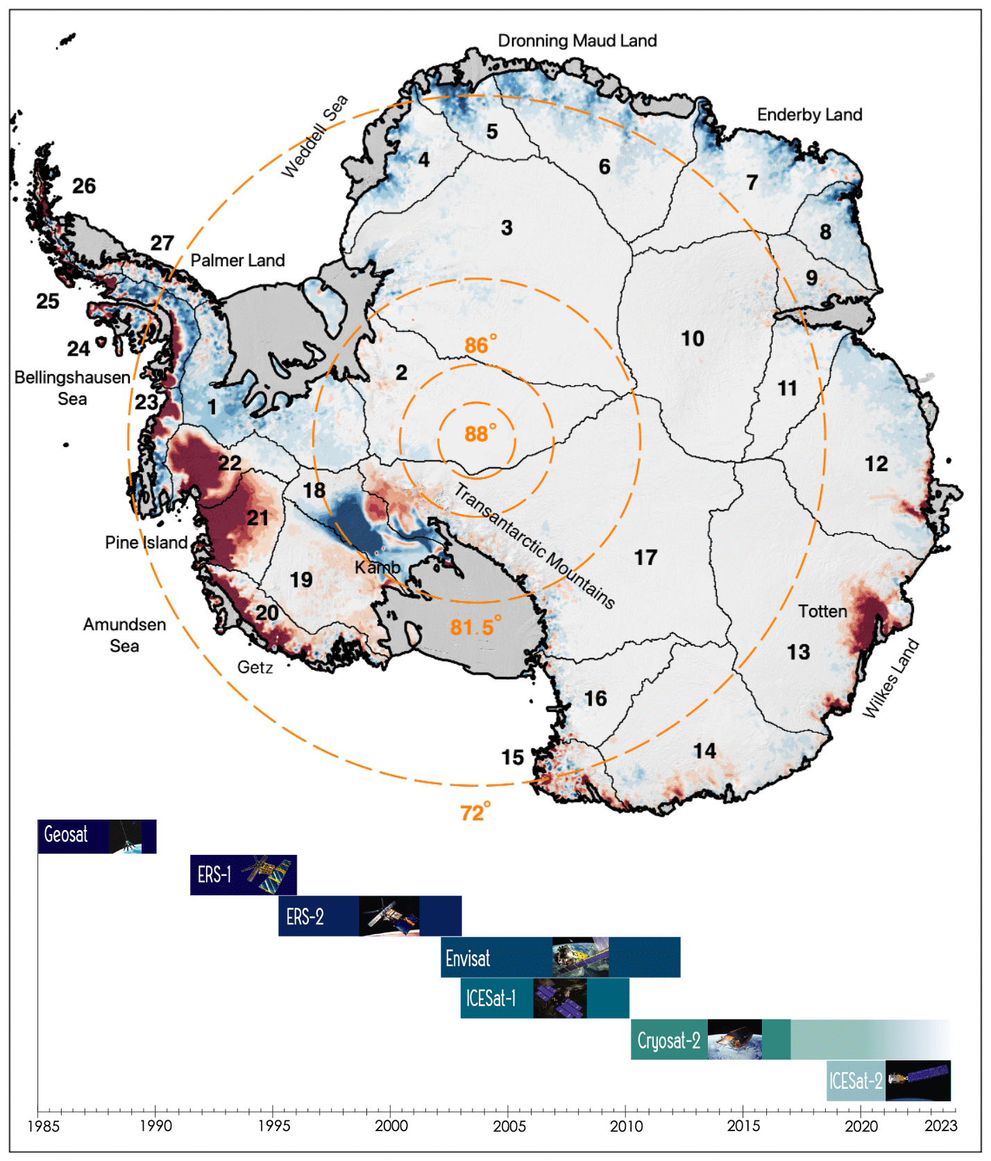
Figure 1Spatial and temporal coverage of the seven satellite altimetry missions used to produce the elevation change synthesis. Concentric dashed circles and labels (orange) indicate orbital limits of each mission (Geosat 72∘; ERS-1, ERS-2, and Envisat 81.5∘; ICESat 86∘; and CryoSat-2 and ICESat-2 88∘). Antarctic drainage basins 1–27 are shown in black (Zwally et al., 2012). Orbital limits and drainage basins are plotted over elevation change rates (1992–2020) from this study, with a range of ±20 cm a−1 (blue indicates positive and red negative changes in elevation).
2.1 Geosat
The U.S. Navy launched the GEOdetic SATellite (Geosat) in March 1985, which operated until September 1989, providing limited Antarctic coverage between ±72∘ latitude. The main goal of the mission was to provide the U.S Navy with detailed information about the marine gravity field. Geosat operations consisted of two separate missions, in which the initial 18 months were the classified “geodetic mission” (GM), in a 135 d repeat orbit ending in September 1986, and the “exact repeat mission” (ERM), in a 17 d repeat orbit lasting until the end of the mission. The mission carried a Ku-band (13.5 GHz) pulse-limited altimeter providing measurements every 670 m along track (10 Hz), with a pulse-limited diameter of ∼ 3 km. In this study we used “ice data record” (IDR) from the Radar Ice Altimetry Group at NASA Goddard Space Flight Center (GSFC) providing geolocated and corrected surface elevations. Only records with a valid retracking correction and waveforms containing a single return echo were used in the study to reduce noise in the derived surface elevations. We detected the presence of a bias in the automatic gain control (AGC) parameter of 1.23 dB between the geodetic mission (GM) and the exact repeat mission (ERM) phases. This is most likely due to the change in orbit, and it did not affect any of the other parameters, including the surface elevation change.
2.2 ERS-1 and ERS-2
The European Space Agency (ESA) launched the European Remote Sensing (ERS) satellites in 1991 (ERS-1) and 1995 (ERS-2), respectively. They operated continuously between ±81.5∘ latitude until 1996 and 2003, respectively. Both missions carried conventional pulse-limited Ku-band (13.6 GHz) radar altimeters, with a pulse-limited footprint of ∼ 1.5 km and an along-track resolution of 370 m (20 Hz sampling rate). The two missions operated in a 35 d repeat orbit, though ERS-1 had several shorter mission phases early on that deviated from the standard repeat-track orbit. For this study the “REprocessing of Altimeter Products for ERS (GDR): 1991 to 2003” (REAPER), detailed in Brockley et al. (2017), is used to obtain surface elevation measurements. This product contains updated corrections and improved calibrations. For each satellite record we separated the data from the two operational modes, “ocean” and “ice”, excluding any data used for calibration. The product provides different retracking solutions from which we have chosen to use the ICE1 retracker, otherwise known as the “offset center of gravity” (OCOG) retracker (Wingham et al., 1986), using a 30 % threshold of the maximum waveform amplitude. The Ku-chirp and the ICE-1 20 Hz quality flags, available in the product, were used to exclude poor-quality observations from the analysis.
2.3 Envisat
The “Environmental Satellite” (Envisat) was launched by ESA in 2002 as a successor to the ERS mission and was officially decommissioned in 2012. Envisat was launched into a 35 d repeat orbit, operating with a pulse-limited radar altimeter with the same footprint, radar frequency, and sample frequency as the earlier ERS missions. For Envisat we used the “RA-2 Geophysical Data Record” (GDR) version 2.1. Only data collected during the period 2002 to 2010 were used due to changes in orbit initiated in October of 2010. The GDR product, as with the REAPER product, includes elevations determined using the ICE-1 retracker with a 30 % threshold of the maximum waveform amplitude, which we used for this analysis. We applied the same quality filter on the GDR records as with the ERS product, using the Ku-chirp and ICE-1 quality flags.
2.4 ICESat and ICESat-2
The National Aeronautics and Space Administration (NASA) launched the Ice, Cloud, and land Elevation Satellite (ICESat) in 2003, which operated from 2003 to 2009 in a 96 d repeat orbit. The mission carried a novel laser altimeter providing a 70 m beam-limited ground footprint, with 170 m along-track sampling (40 Hz). We used the latest version of the GLAS06 product (release 34), which has been corrected for the “Gaussian centroid offset” (Borsa et al., 2014) and detector saturation and converted to heights above the WGS84 ellipsoid. We did not apply any inter-campaign bias to the ICESat elevations as there is no consensus that these are required (Borsa et al., 2019). The records are further edited to remove poor-quality observations using the accompanying quality flags (elev_use_flh >0, sat_corr_flg >2, sigma_att_flg >0, i_numPk >0).
The ICESat-2 mission is a follow on mission to ICESat and was launched in October 2018 with the goal of continuing the long-term altimetry measurements of polar regions (Markus et al., 2017). It carries a new and novel photon counting laser altimeter that uses a 532 nm laser with a pulse repetition rate of 10 kHz and that operates in a repeat-track configuration over the continental ice sheets. In contrast to its predecessor's single beam, ICESat-2 collects ground measurements using six individual laser beams arranged in three pairs. Each of the beam pairs is separated by 3 km and each inter-pair beam by 90 m across track. This configuration allows for a direct estimate of the across-track surface slope that was not directly possible with ICESat's single beam configuration. The beam limited footprint for each beam is 12 m in diameter sampling every 0.7 m along track with a repeat frequency of 91 d. In this study surface elevation from the ATL06 product was used following the approach outlined in Smith et al. (2019, 2020). Here a segmentation filter (difference filter) was used to remove poor-quality observations if differences between consecutive points exceed a threshold of 2 m the point was rejected. Further editing was done using the ATL06 quality flag, keeping only data designated to be of good quality (“atl06_quality_summary = 0”).
2.5 CryoSat-2
ESA's CryoSat-2 mission launched in 2010 with the primary purpose of monitoring changes in Earth's sea and land ice. This satellite carries a new type of delay Doppler radar altimeter (Raney, 1998) equipped with a dual antenna configuration allowing for interferometric measurements of surface elevations. The altimeter system, referred to as SIRAL, operates in two different modes over the ice sheets: a synthetic aperture radar interferometric (SARIn) mode over the marginal areas and a low-resolution mode (LRM) (a conventional Ku-band pulse-limited radar – identical to ERS and Envisat) over the ice sheet interiors. The Doppler/delay radar allows for increased along-track resolution compared to conventional pulse-limited altimetry. The SARIn mode has an effective resolution of 350 m along track and 1500 m across track, compared to the LRM modes' 1500 m along- and across-track resolution. Further, the dual antenna configuration allows for mapping of the exact position of the surface echo location by estimation of the across-track look angle from the difference in path length of the signals between the two antennas. In contrast to previous missions, CryoSat-2 operates in a drifting orbit, with a 369 d repeat and a 30 d sub-cycle. The drifting orbit offers improved spatial coverage compared to repeat-track orbits at the expense of larger across-track distances. We processed both the LRM and SARIn modes using the ESA L1b Baseline-C product for the time span 2010–2018 using a custom CryoSat-2 processor described in Nilsson et al. (2016). For the LRM mode we have chosen to use a 10 % threshold of the maximum waveform amplitude for retracking, similar to Schröder et al. (2019).
To generate a continuous record of elevation change for Antarctica several corrections and processing steps need to be applied to the altimetry data. The details of the different steps are provided in this section, and a summary of the corrections their order of application is provided below:
-
application of geophysical corrections and parameter editing for each mission (Sect. 2)
-
correcting for slope-induced error in the radar altimetry using an ancillary elevation model (Sect. 3.1)
-
removal of the static topography to extract time-variable elevation change (Sect. 3.2.1)
-
correcting the radar altimetry data for changes in near-surface scattering conditions (Sect. 3.2.2)
-
cross-calibration and integration of the multiple sensors and modes into a continuous time series (Sect. 3.2.3)
-
normalization of seasonal amplitudes for each sensor using a reference mission (Sect. 3.2.4)
-
interpolation, extrapolation, and filtering to create a three-dimensional data product (Sect. 3.2.5).
3.1 Slope-induced error correction
The largest source of error in radar altimetry over ice sheets is associated with the effects of surface slope inside the beam-limited radar footprint. This error stems from an inability to locate the surface from which most of the echo power originates (off nadir). Because of this, the echo is assigned the location of the sub-satellite point on the Earth surface. This introduces a slope-dependent measurement error on the order of 0–100 m (Brenner et al., 1983), which varies with the magnitude of the surface slope. There are a few ways of minimizing the slope-induced error (Bamber, 1994; Roemer et al., 2007). For this study we used the “relocation method” described in Nilsson et al. (2016). The relocation method corrects both the range and the coordinates to the echolocation (from nadir) using topographical information, such as surface slope, aspect, and curvature. This method has been shown to improve surface elevation retrievals compared to other approaches (e.g., Schröder et al., 2017). To compute the required surface slope, aspect and curvature, we used the “bedmap2” digital elevation model from Fretwell et al. (2013) resampled to 2 km horizontal resolution.
3.2 Elevation change estimation and algorithms
Surface elevation changes are determined as follows: the local mean topography within a specified search radius is removed from each mission and mode, leaving only the elevation anomalies that contain the time variable signal. Artificial trends and seasonal amplitudes in elevation anomalies that are introduced by changes in surface scattering characteristics are reduced proportionally to the correlation with the received radar waveform shape. Intermission biases in seasonal elevation anomalies are further minimized using a normalization scheme that references all seasonal elevation change amplitudes to those observed by CryoSat-2. A cross-calibration scheme is applied to adjust and merge elevation change from all missions and modes into a continuous monthly time series. Lastly, interpolation is used to generate a consistent gridded product with 1920 m horizonal resolution at monthly time steps from 1985 to 2020. The details of each step are provided in the following sub-sections.
3.2.1 Removal of time-invariant topography
To create time series from observations of surface elevations, the time-invariant topography must be removed to obtain the change signal. This can be done by directly modeling the topography at any given position, e.g, by fitting a mathematical surface using least squares, while accounting for the spatial and temporal trends. This rather simple approach, however, has some inherent limitations. When solving for time-invariant topography one must account for discrepancies between observations originating from (1) differences in the orbital geometry of the missions, (2) differences in ascending versus descending range estimates, and (3) differences in measurement density. To account for (1) we employ an iterative prediction-point adjustment to solve for the topography given a pre-defined grid of a specified dimension for ascending and descending tracks separately for each mission or mode. For each grid node, the closest data points inside a specified search radius are used to compute a new centroid location when five or more data points are available. This centroid location is used in the next iteration as the new prediction point. This allows us to conveniently follow the reference orbits (locations of highest data density) to solve for the topography along the satellite ground tracks. Issue (2) has been handled in different ways (e.g., Flament and Rémy, 2012; McMillan et al., 2014; Moholdt et al., 2010). We have chosen to solve (2) by separating the individual datasets in ascending and descending orbits, solving for the topography at the same center date with the inclusion of a linear trend. The differing number of available observations (3) in each independent solution is handled by allowing for a different number of coefficients in the mathematical surface topography model that is fit to the data. We have provided three different mathematical models of topography (including time) that vary spatially depending on the number of data points available in the local search area at the grid node.
For locations with 15 or more observations a biquadratic surface (six coefficients) is modeled. When 5 to 14 observations are available, a bilinear surface (three coefficients) is modeled. If there are less than five observations, the local mean (one coefficient) is removed, and the slopes are estimated independently in each direction (x and y). The linear temporal term in the design matrix is used to center the data to a specific time and is always included, except if n<5 points. A robust least-squares approach, M estimator (Huber's T weighting function), is used to solve for the model coefficients (Holland and Welsch, 1977).
Time-invariant surface topography is estimated at each prediction point and removed from the original observations inside each local search radius (excluding the linear term). This produces topographic residuals varying only with time. Using this approach, it is common for the search radius of different along-track centroids to overlap. This can produce situations for which a node, with corresponding elevation data, might already have been provided with a solution. To ensure that the best time-invariant topography solution is retained, the new correction is only applied if the estimated root mean square (RMS) of the residuals (with respect to the time-invariant topography) is lower than the previously computed solution for the data point in question.
We select different search radii for the repeat-track (ERS-1, ERS-2, Envisat, ICESat, Geosat) and drifting-track (CryoSat-2) missions. The radius is empirically determined by investigating the residual RMSE from the algorithm over different types of surfaces. We found that, on a 500 m grid spacing, a search radius of 500 m provided a good trade-off between the accuracy and computational efficiency of the algorithm for the repeat-track missions. For CryoSat-2 and Geosat, we found that a higher search radius of 1000 m was needed to provide results with a comparable RMSE. This larger search radius allows for more ground tracks to be included in the inversion, reducing the variance of the model residuals. The inclusion of a linear temporal trend in the fit is key to effectively remove the ascending/descending bias and to center all data to a common epoch (center date of each mission or mode).
3.2.2 Surface and volume scattering correction
The microwave pulses transmitted by spaceborne radar altimeters at Ku-band frequency (∼ 13.6 GHz) are sensitive to changes in the dielectric properties of the ice sheet surface (as determined by changes in the snow grain size, temperature, density, and water content, among others). Large-scale temporal and spatial changes in the scattering horizon induce changes in measured range, and thus surface elevation, and can introduce long-lived biases in the derived elevation change rates (Arthern et al., 2001; Davis and Ferguson, 2004; Khvorostovsky, 2012; Nilsson et al., 2015b; Wingham et al., 1998). To mitigate this effect, we use a retracking algorithm that tracks the leading edge of the return waveform (i.e., a maximum amplitude threshold between 10 % and 30 %). Such retrackers have been shown to be less sensitive to changes in ice sheet surface properties (Helm et al., 2014; Nilsson et al., 2016; Schröder et al., 2017). Another key step is removing elevation variability that is correlated with changes in the received radar waveform shape (Flament and Rémy, 2012; McMillan et al., 2014; Paolo et al., 2016; Simonsen and Sørensen, 2017; Zwally et al., 2005). The shape of the waveform is intricately linked to the medium in which it is propagated or reflected. Removing the correlation between changes in the shape of the radar waveform with elevation can largely reduce these artificial signals. For this study we approximated the shape of the radar waveform following the definition of Flament and Rémy (2012) and Simonsen and Sørensen (2017) using the backscatter (Bs), the leading-edge width (LeW), and the trailing edge slope (TeS).
The spatially variant scattering correction was estimated by computing the local sensitivity gradient (SG) between each waveform parameter and elevation residuals using a multi-variate least-squares inversion. The SG parameters were estimated for ascending and descending tracks separately. All waveform parameter time series were centered and normalized using the mean and standard deviation. Further, parameters were detrended by applying a difference operator, forming the following least-squares model:
where ∇ is the difference operator, h the elevation residual (elevation relative to time-invariant topography), σ the standard deviation, and the overbar the average value of the parameter.
The SG parameters were inverted for using the same adaptive search center approach as described in Sect. 3.2.1. The estimated SGs were then used to correct each observation within the search cap using the linear combination of the original waveform parameters and the estimated coefficients. Finally, we apply a linear space–time interpolation to estimate corrections at locations where the multi-variate fit did not provide a satisfactory solution.
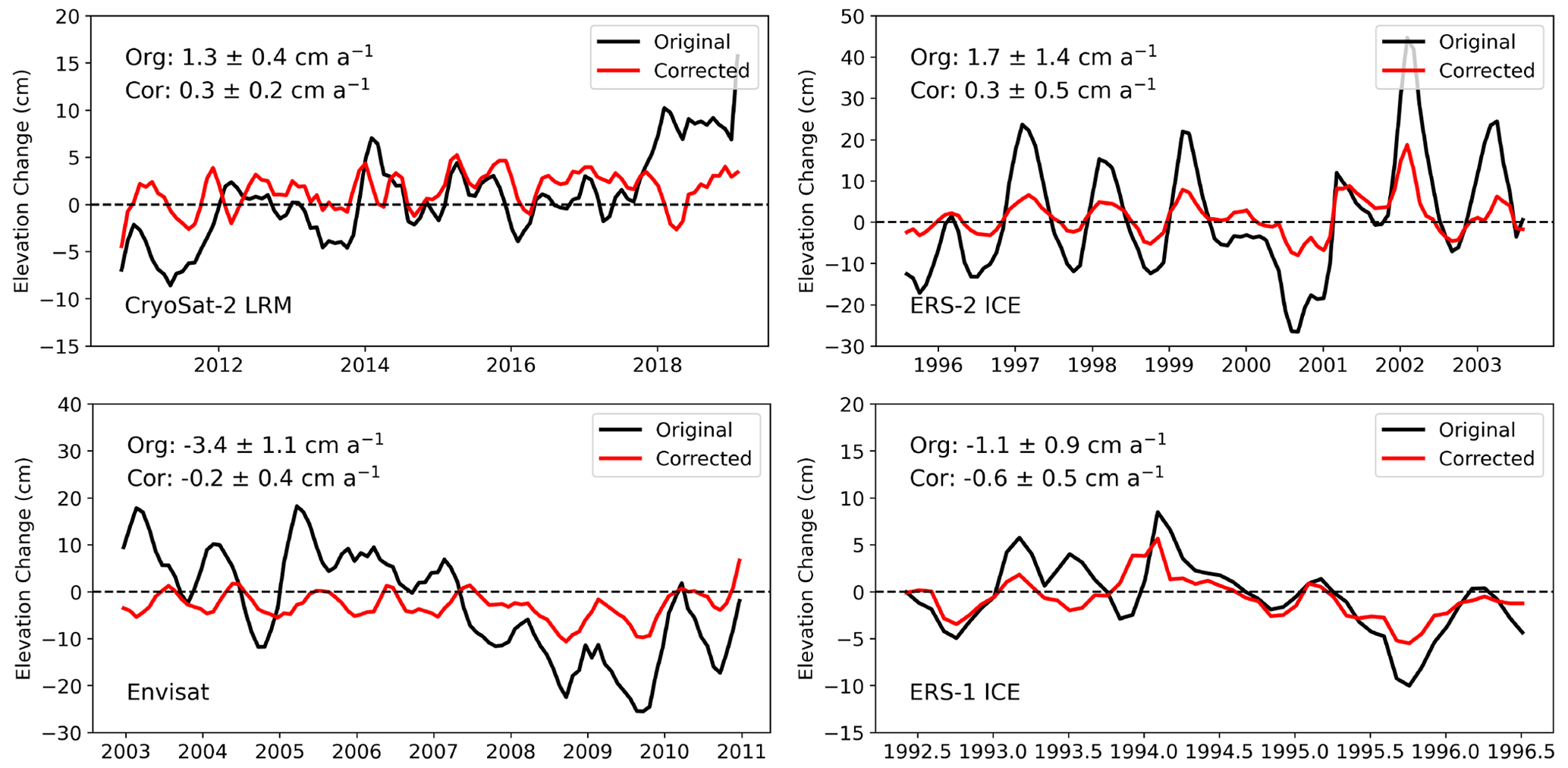
Figure 2Original and scattering corrected area integrated time series for Lake Vostok in East Antarctica, which has been shown to have a height trend close to zero over recent decades (Richter et al., 2014). A discrepancy in uncorrected height trends is observed for the various missions due to differences in altimetry processing, orbit configuration, and the quality of the geophysical corrections. Envisat and ERS-2 (Ice) show the largest uncorrected magnitude in both trend and seasonal signal. Corrected height change records show significantly lower seasonal amplitudes and trends that are close to zero.
To determine the optimal search radius for generating the scattering correction, we performed a sensitivity study over Lake Vostok in East Antarctica (Fig. 2). Lake Vostok was selected due to its low surface slope, on average 0.03∘, and highly stable surface (Richter et al., 2014), minimizing the impact of the static and time variable topography in the analysis. After varying the search radius from 1 to 5 km, we found that the 1 km solution provided the most accurate trend and seasonal amplitude for all missions and modes. We also found that the absolute magnitude of both the trend and amplitude increased linearly as the search radius increased. We interpret this result as a decrease in the efficiency of the correction possibly due to de-correlation with increasing spatial and temporal scales. The use of a 1 km search radius is also computationally efficient as fewer data are used in the inversion. Applying these lessons to the ice-sheet-wide processing, we found that the correction has a minor impact on the estimated trend for the CryoSat-2 SARIn mode and the Geosat missions. We also found that the application of the correction to the SARIn and Geosat data increased the seasonal amplitude of the local (single grid cell) time series (Sect. 3.2.4). Given that there is no physical justification for an increase in seasonal amplitude, we chose not to apply the correction to the Geosat mission and the SARIn-mode data. For the other missions, the magnitude of the correction varied across missions and modes of operation, in which the largest changes in trend and amplitude were found for Envisat and ERS-2 Ice mode and the lowest for CryoSat-2 LRM. By examining the changes in trend and amplitude we found significant spatial patterns, also varying across each mission and mode, as shown in Fig. 3. These patterns show strong correlations to both surface slope and roughness and signals of metrological origin (Armitage et al., 2014) and are mostly driven by katabatic winds and the re-distribution of snow. The wind effect can be observed in the RMSE plots for Envisat and for ERS-2 Ice as banded patterns in the East Antarctic sector following the main ridge lines.
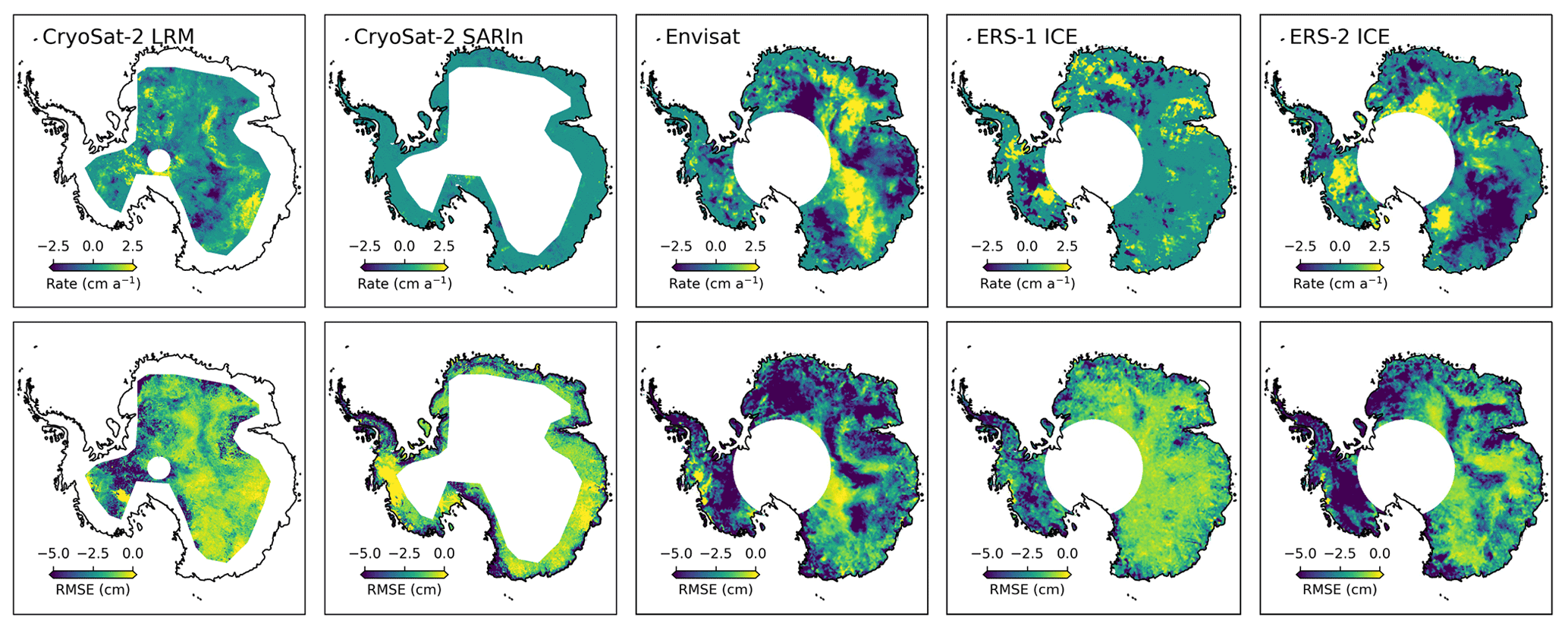
Figure 3Change in elevation change rate and RMSE (seasonal amplitude) of the local time series after correction for temporal changes in scattering (penetration depth). Spatial patterns linked to surface conditions can be clearly observed. These effects are most prominent for Envisat and ERS-2.
3.2.3 Cross-calibration and integration
Removal of the time-invariant surface topography is done internally to each dataset such that elevation residuals are not aligned to the same surface (see Sect. 3.2.1). To align elevation anomalies to a common reference we first solve for intermission offsets. These offsets vary regionally (Khvorostovsky, 2012; Wingham et al., 2009; Zwally et al., 2005), depending on the underlying topography, physical interactions of the radar with the surface, and differing retracking methodologies. In contrast to previous studies (e.g., Davis and Ferguson, 2004; Davis, 2005; Khvorostovsky, 2012; Li and Davis, 2006; Schröder et al., 2019; Wingham et al., 2006, 2009; Zwally et al., 2005), we estimate these offsets using a least-squares adjustment. This approach allows for a simple, yet consistent, alignment of multiple relative elevation anomalies without requiring full overlap between missions to solve. The technique follows the approach of Bevis and Brown (2014), using the entire multi-mission record to constrain the solution while accounting for trend, seasonality, and intermission or mode offsets. The trend is represented by a polynomial, with a maximum order of six, a four-term Fourier series to account for seasonality, and Heaviside functions to solve for the intermission offset between missions and modes. The design matrix can be written as follows:
where np is the model order, t is the time in decimal years, tr is the reference time in decimal years (tr=2013.95), Tk is the seasonal period reference (T1=1 and T2=0.5), nf is the number of Fourier series terms (nf=4), and nj is the number of missions and modes (nj=10).
Here, we add offsets for 10 different missions and modes in the least-squares model (Geosat, ERS-1 Ocean and Ice, ERS-2 Ocean and Ice, Envisat, ICESat, CryoSat-2 LRM and SARIn, and ICESat-1) to all data falling within the search radius. To determine the order of the polynomial we use the Bayesian information criterion (BIC; Schwarz, 1978) to select the polynomial that produces the lowest BIC value estimated from monthly binned data.
The cross-calibration is performed on a 2 km polar-stereographic grid (EPSG: 3031) using a variable search radius of 1–10 km surrounding each grid cell. The radius is increased until 70 % of the time series is filled (monthly) or the maximum radius is reached. If the maximum search radius is reached and the 70 % criterion is not meet, we continue processing using all available data. In most cases the search radius is in the range of 2–10 km. Outliers in the original time series were initially removed using a 1-year running median filter in which values larger than 10 times the median absolute deviation (MAD) were rejected. The model is then fit to the time series using a robust least-squares inversion as in Sect. 3.2.1. Solutions are rejected if the absolute value of the linear rate is larger than 20 m a−1 or if the RMS of the time series relative to the model is larger than 4 m. If any of the derived offsets are larger than 100 m, the offset is set to zero. The offsets estimated from the least-squares inversion are then subtracted from the time series providing an initial cross-calibrated record of elevation change. Further, a last outlier step is performed in which the model is used to filter the time series by omitting observations exceeding 10-times the MAD of the model residuals.
This approach has several advantages; it allows a first-order calibration of non-overlapping time series while also aligning overlapping missions and modes to their common mean. To account for time series that do not fully conform to our choice of a linear model, a secondary cross-calibration is performed for the four mission-specific offset coefficients (ERS-1 to ERS-2, ERS-2 to Envisat and ICESat, Envisat and ICESat to CryoSat-2, and CryoSat-2 to ICESat-2), using the post-fit model residuals. This approach was chosen as it facilitates the estimation of any residual offsets after removal of the majority of the trend and seasonality, making it simple to estimate the overall bias between the mission groups. The offsets for groups ERS-1 to ERS-2, ERS-2 to Envisat and ICESat, and CryoSat-2 to ICESat-2 were estimated by taking the median difference between the two datasets over their respective overlapping time periods. This approach was found to be suboptimal for the Envisat and ICESat to CryoSat-2 offsets due to the short period of overlap (less than 4 months) and large changes during the time period 2009–2011. To overcome this limitation, we applied three different methods, generating five different independent Envisat and ICESat to CryoSat-2 offsets at each search node. For method 1, we fit two second-order polynomials to the two residual time series and compute the median offset between the two functions over a 1-year overlap (2010–2011), as well as the difference between the two intercepts of the polynomials. For method 2, we applied a Kalman smoother with a state-space model consisting of a constant local level and a random walk trend (Kalman, 1960; Shumway and Stoffer, 1982) that better accommodate the variability in the time series. The filter was initialized with a variance rate of 1 mm2 a−3 (Davis et al., 2012), with the observational noise given by the RMSE of each residual time series. Initial state values of the filter were set to zero for both the level and trend with large initial uncertainties (1×10⁶). The filter parameters were then optimized using the expectation__maximization (EM) algorithm (Shumway and Stoffer, 1982) with five iterations. The same approach as in Method 1 was used to generate the two estimates of the offset based on the 1-year overlap and the differencing of the two intercepts. For method 3, here the offsets were determined by computing the median difference between the two missions over the 2010–2011 time period. To determine which of the offsets produces the best cross-calibration, we apply each offset and compute linear rates of change from 2003 to 2019. These rates are then compared to rates estimated from unbiased ICESat and ICESat-2 measurements produced by Smith et al. (2020), and the offset with the smallest absolute difference was selected. Finally, the selected offset rate difference (radar minus laser) is checked against the difference computed without a residual cross-calibration. If the applied offset did not improve the rate compared to the ICESat and ICESat-2 record, then the residual offset was set to zero. Following Schröder et al. (2019), we remove outliers in the offsets using a 100×100 km 5-MAD moving spatial filter. The intermission offsets are then interpolated using a Gaussian kernel with a 20 km correlation length using the nine closest data points. This produces a spatially consistent field of offsets for the cross-calibration of the elevation residuals. Then the offsets estimated from the initial least-squares adjustment and the offsets estimated from the secondary residual calibration are then applied to create a fully calibrated local time series. Finally, the individually calibrated elevation time series for each mission or mode are averaged to monthly estimates of elevation change for each spatial grid cell, with an associated standard error. Once, the time series have been calibrated a seasonal amplitude correction is applied to the data to normalize amplitudes between missions. This is described in more detail in Sect. 3.2.4. Finally, the monthly normalized time series are then combined and integrated into a continuous record using the weighted average of the data within each overlapping temporal bin. Weights are specified as the inverse variance of each mission's accuracy and the random error estimated from the monthly averaging procedure (see Sect. 4.1).

Figure 4Maps of the residual cross-calibration offset and the corresponding error for the three main intermission transition periods. One should note that here ICESat has been grouped with Envisat in the initial calibration.
The initial least-squares adjustment provided good alignment between overlapping modes (ocean–ice mode) and missions (Envisat and ICESat), as well as a first-order correction for the three weakly overlapping missions that allows for better estimation of the residual biases from the detrended data. Initial offsets were determined to be as large as 10–15 m in areas of rapid change such as Pine Island Glacier. However, the least-squares adjustment was shown to be inadequate when large non-linear elevation changes are present. The magnitude of the estimated residual cross-calibration error (after least-squares adjustment) (Fig. 4) shows that most overlapping regions have a clear correlation with temporal coincident elevation change rates. This pattern is evident in the Envisat to CryoSat-2 transition (Fig. 4) for Dronning Maud Land (basins 5–8), Wilkes Land (basins 12–13), Bellingshausen Sea (basins 23–25), and the Amundsen Sea sector (basins 20–23) (Fig. 10: 2010–2012). For the ERS-2 to Envisat transition, we find a clear correlation between the magnitude of the offsets and the changes in elevation due to variations in surface mass balance in Wilkes Land (basins 12–13 seen in Fig. 1) over the 2001–2003 time period (Schröder et al., 2019).
3.2.4 Normalization of seasonal amplitude
The radar signal's interaction with the surface and sub-surface firn layers can create artificially large seasonal amplitudes and trends, as described in Sect. 3.2.2. We correct for these as best as possible using information contained in the waveform parameters. However, in many cases these corrections are unable to fully correct the artificial signals. This behavior can be seen in Schröder et al. (2019) and in our data, and even after the scattering correction has been applied there exist intermission variations in seasonal amplitude (Fig. 5). To further reduce this effect, we apply an amplitude correction (hn) to each mission to normalize the seasonal signal over the entire record. We normalized the seasonal amplitudes of the ERS-1 and ERS-2 and Envisat records to match amplitudes computed from CryoSat-2. CryoSat-2, which is retracked with a much lower threshold of the maximum waveform amplitude (10 %) for LRM and a maximum gradient threshold for SARIn, has been shown to be less sensitive to changes in surface properties and produces seasonal amplitudes of the same magnitude as ICESat (Fig. 5) (Nilsson et al., 2016). After removal of the long-term trend, the amplitude normalization was computed for each mission, except for ICESat and CryoSat-2, according to
where (ai) is the amplitude of the mission (), (ar) is the reference amplitude estimated from CryoSat-2 data, and are the coefficients for the seasonal model. The correction is applied by subtracting it from each individual time series, and the normalization has the effect of producing more homogeneous amplitudes over the entire altimetry record. The application did not introduce any noticeable shift in the phase of the seasonal signal.
ICESat and CryoSat-2 LRM mode shows a similar magnitude in amplitude and supports the choice of using CryoSat-2 as reference in which the difference is most likely explained by the lower temporal sampling of ICESat. The slightly lower seasonal amplitude of ICESat-2 is mostly likely due to the short time span used to estimate the amplitude (2 years), as seen in Fig. 5.
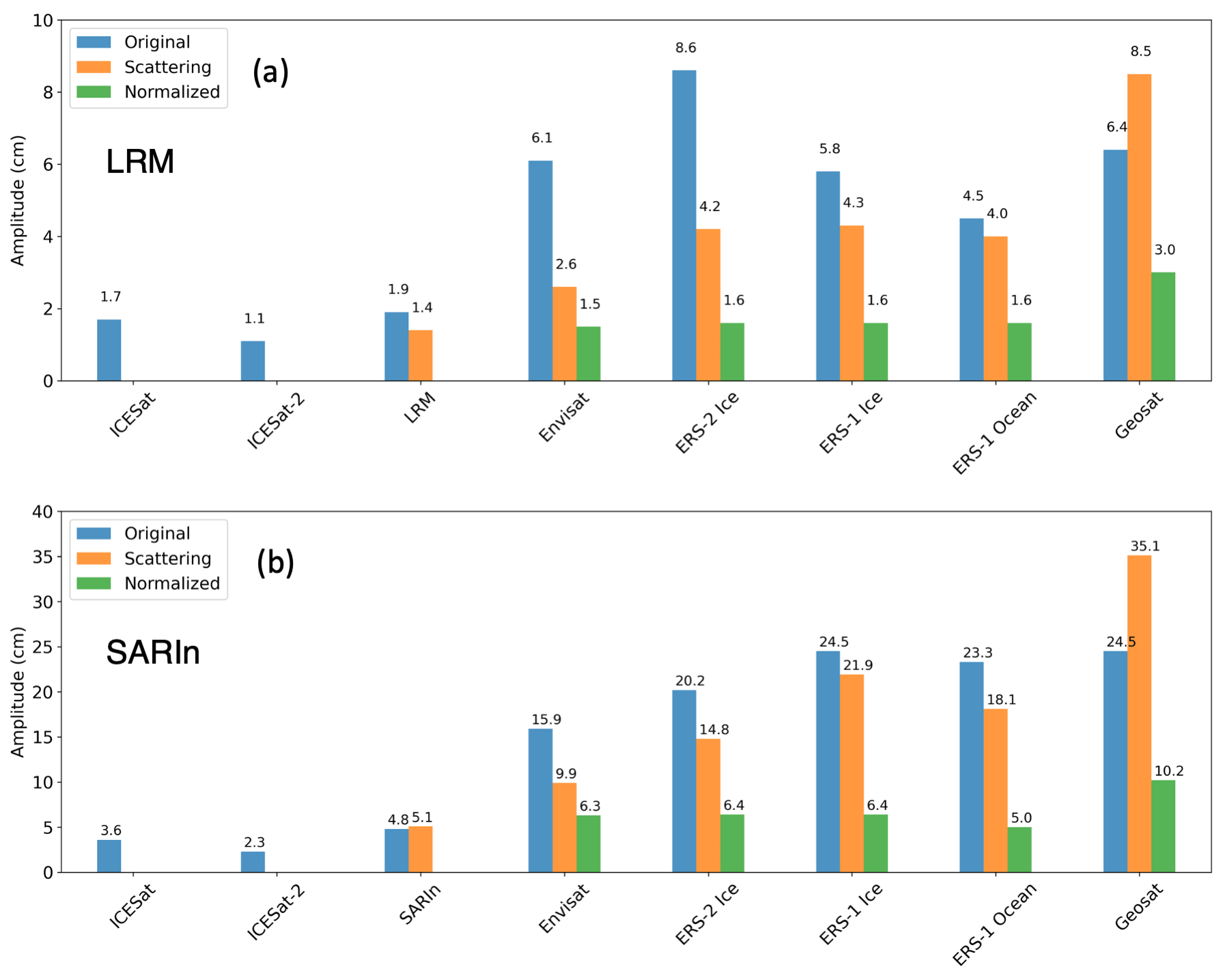
Figure 5Median seasonal amplitude of the different missions and modes for the CryoSat-2 LRM (a) and SARIn (b) mode masks (south of 81.5∘ S for LRM). The blue bars show the original seasonal amplitude with no corrections applied, the orange bars show the amplitude once the mission-dependent scattering correction has been applied, and the green bars show the normalized amplitude after adjustment using CryoSat-2 as reference.
3.2.5 Interpolation, extrapolation, and filtering
Collocation (a.k.a. ordinary kriging; Herzfeld, 1992; Nilsson et al., 2016) was used to interpolate the monthly elevation change estimates onto a 1920 m grid using a maximum search radius of 50 km and a 20 km correlation length. The value of 1920 m was chosen to be consistent with the ITS_LIVE grid that accommodates nesting of datasets at multiple resolutions. An adaptation to Nilsson et al. (2016) is that the local average is replaced by an estimate from a linear model regressed against both surface elevation (bedmap2) and surface velocity from Gardner et al. (2019) (available at https://its-live.jpl.nasa.gov, last access: 4 May 2022), following the approach of Hurkmans et al. (2012) as seen below:
where hDEM is elevation values from the digital elevation model (DEM; bedmap2), and (v) values are the surface velocity values. The minimum surface velocity is capped at 50 m per year to avoid introducing noise in the interior parts of the ice sheet, and the logarithm is applied to linearize the range of velocity values.
For the interpolation, the spatial variance is taken to be the mean of the random error estimated from the monthly averaging procedure. The noise term (diagonal of the error matrix) used in the collocation to weight each observation is taken as the root sum square (RSS) of the variance of the cross-calibration error, mission accuracy, and the random error (see Sect. 4.1). Further, a minimum error of 5 cm is given to all observations based on ICESat and ICESat-2 crossover analysis (Sect. 5.1, Table 1). Prior to the interpolation we remove erroneous observations using a 100 km radius spatial filter centered at the location of each data value. In this procedure, following Smith et al. (2020), we remove spatial gradients inside each 100 km cap by fitting a biquadratic surface, and if the observation exceeds a specific threshold, it is removed. This threshold is dependent on the local surface roughness and elevation change rate, in which the surface roughness is estimated from the bedmap2 DEM. If the surface roughness is larger than 60 m and the absolute elevation change rate is less than 0.2 m a−1 (Smith et al., 2020), then the filter threshold is set to 3-MAD; otherwise it is set to 30-MAD (gross outliers). This has the effect that the filter is more aggressive in regions of steep topography (Antarctic Peninsula and the Transantarctic Mountains) while preserving the signal in areas of rapid change. In the temporal domain, and after spatial interpolation, a 12-month median filter is applied to remove outliers exceeding the 10-MAD threshold. Rejected values in the time series are filled using a Gaussian kernel with a correlation length of 3 months.
Differences in satellite orbits cause spatial coverage to vary from 81.5 to 88∘ S (excluding Geosat that only reached 72∘ S). The large gap in coverage between the maximum latitude reached and the south pole is referred to as the pole hole. To create a spatially complete record of elevation change we use extrapolation to fill the pole hole for each monthly time epoch. We first average each monthly spatial field to a coarse 20 km resolution, corresponding to the average correlation length of the elevation anomalies. We then fill the CryoSat-2 and ICESat and ICESat-2 pole holes using our collocation–kriging algorithm (with velocity and elevation terms set to zero), similar to Zwally et al. (2015), using the 200 closest 20 km averaged values and with a correlation length of 100 km, and we provide each averaged observation with the aggregated error within each cell. For the 81.5∘ S missions (ERS-1 and ERS-2 and Envisat) the unobserved area is about 18 times larger than the area for CryoSat-2, ICESat, and ICESat-2. This makes our extrapolation approaches less useful. To overcome this issue, we remove a linear trend and the annual seasonal signal estimated over the ICESat, CryoSat-2, and ICESat-2 period for each grid cell over the 1992–2020 period. The residuals to this model are more homogeneous in the far field. We then extrapolate these residuals to the entirety of the 81.5∘ pole hole for each month using the same spatial kriging–collocation algorithm as previously used (velocity and elevation set to zero). After the monthly residuals have been gridded and filled, we add back the linear trend and seasonality estimated from the CryoSat-2, ICESat, and ICESat-2 model for each location. For both approaches we multiply the predicted errors from the algorithm by a factor of 3 to avoid errors that are too small (e.g., less than 5 cm as estimated from ICESat-2 as in Table 1). The estimated errors for the pole hole are to be considered only as a guide. These errors are based on the error statistics of the surrounding 20 km averaged data and errors being extrapolated inward to the pole, such as data from the Transantarctic Mountains. This can provide a somewhat unrealistic looking spatial pattern for the estimated error field but one which is still based on observations.
Interpolated elevation anomalies can easily be included or excluded in any future analysis using the data_flag field that is included with the data product: 0 = no data, 1 = high-quality data, 2 = low-quality data, and 3 = pole hole. The “low-quality data” index is based on a minimum bedmap2 surface roughness criterion that is set to the approximate size of the range gate window of the radar altimeters (roughness threshold for Geosat: 30 m; ERS-1, ERS-2, and Envisat: 120 m; and CryoSat-2: 240 m). We also provided the ESA COP DEM (https://spacedata.copernicus.eu/web/cscda/dataset-details?articleId=394198, last access: 4 May 2022) resampled to our 1920 m grid using a box filter (averaging) to allow the user to investigate time-evolving topography. Center date of the DEM is circa 2010–2015, which is in line with our provided center or reference date of 16 December 2013.
To estimate volume changes at the basin scale (Fig. 1), we replaced the interpolated values flagged by the surface roughness criterion with values estimated from a hypsometric relationship (Moholdt et al., 2010; Nilsson et al., 2015a). Here, the monthly values of elevation change (excluding the values flagged by roughness) were binned using the median value within 100 m elevation intervals according to the hypsometry provided by the DEM (bedmap2). As in Morris et al. (2020), a linear model was fit to these binned values and used to extrapolate values to areas flagged as “low-quality data”. This was done only for the purpose of this paper and is not applied to the final data product. This choice was made to allow the users to select a suitable method given their interest or constraints.
4.1 Uncertainties of elevation change time series and data
An internal crossover analysis was performed to determine the relative accuracy of each mission and mode in a similar manner as Brenner et al. (2007) and Schröder et al. (2019). We estimated the standard deviation of all crossovers with a time difference of less than 31 d. Crossovers were binned as a function of surface slope at intervals of 0.04∘ (Fig. 6). The relative accuracy of each mission or mode was determined from the standard deviation at zero slope by fitting an error function (inside an interval of 0–0.4∘) as shown in Table 1. To derive the uncertainty of each time series epoch we use the spatiotemporal variability inside each monthly time interval in the form of the standard deviation. This provides a random error for each monthly value that varies both in space and in time and encompasses measurement-related errors driven by topography, retracking, range corrections, etc. To quantify the total cross-calibration error for each time series we use the standard deviation of each grouped mission offsets (Sect. 3.2.3) and add them in quadrature to estimate the total cross-calibration error, similar to Schröder et al. (2019). We then have the total error (σm) for each month in each time series by summing the individual error sources as follows:
where (σm) the error due to the elevation change variability within each monthly interval for each time series, and (σc) is the total cross-calibration error for each time series. The estimated total error () is the provided RMS error in the product (varying both by location and time).
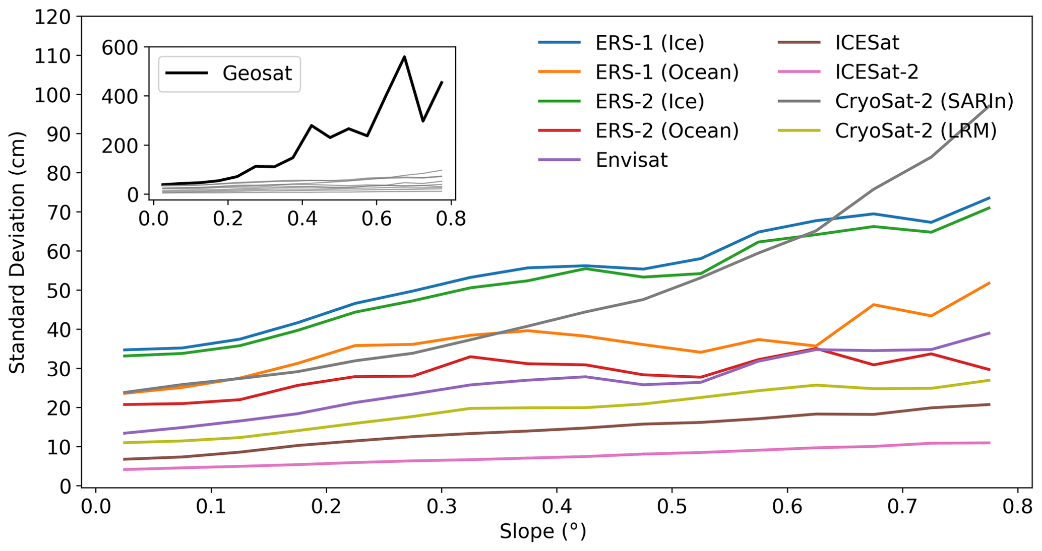
Figure 6Standard deviation (cm) of intra-mission and intra-mode crossovers for the Antarctic Ice Sheet as a function of surface slope (degrees). Precision decreases quasi-linearly as surface slope increases.
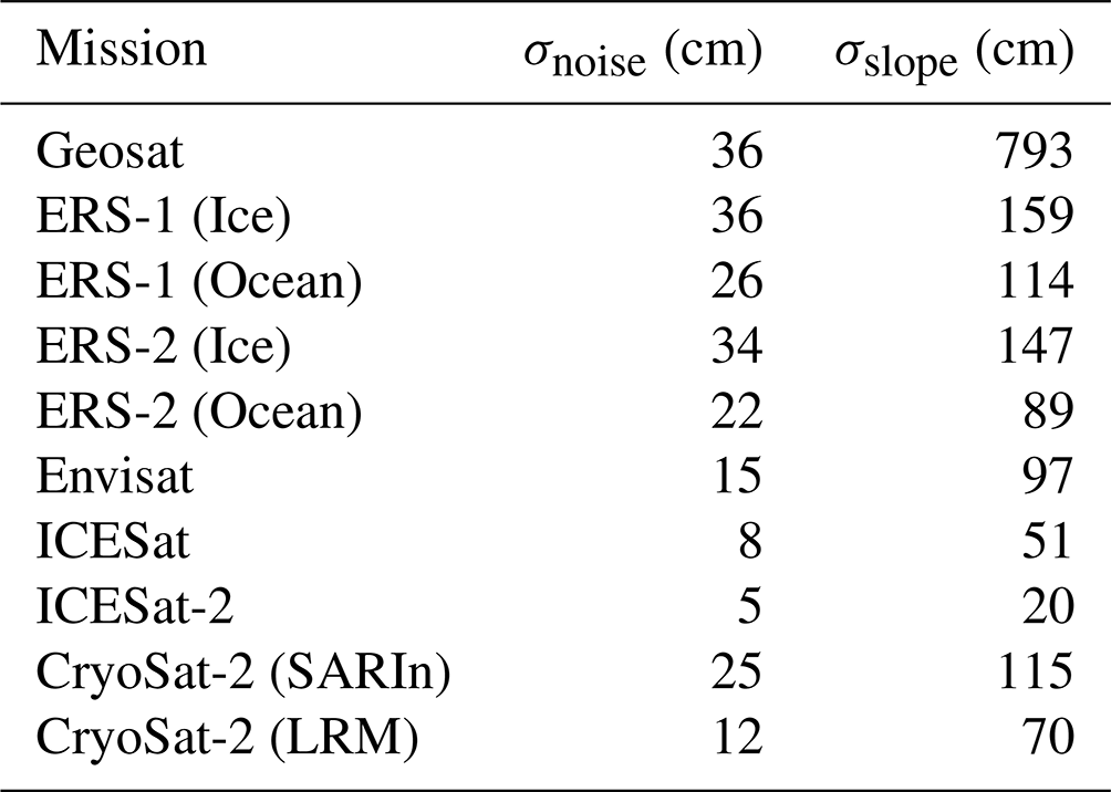
Table 1Sensor and mode errors (σmission) as a function of the random (σnoise) and slope-dependent (σslope) errors. Slope (α) is in degrees. Modeled error (σmission) is based on fitting the following function to the intra-sensor, intra-mode crossover data: .
4.2 Validation of rates of elevation change
To validate the data product, we computed elevation change rates and compared them to rates derived from near-coincident Operation IceBridge (OIB; MacGregor et al., 2021) and pre-OIB data spanning the period 2002 to 2019 using the Airborne Topographic Mapper (ATM; MacGregor et al., 2021) laser altimeter. Elevation change rates for ATM were derived following the approach of Nilsson et al. (2016), in which a linear model was solved at each measurement location using a search radius of 175 m. Following the approach of McMillan et al. (2014) and Wouters et al. (2015), the local slope was used to correct the measurements to the reference track, indicated as Track_Identifier = 0 in the product. Solutions were rejected if they contained fewer than two campaigns of ATM data, the magnitude of linear rate was larger than 10 m a−1, the standard deviation of the solution exceeded 1 m a−1, or if the solution contained fewer than 10 measurements, as well as if the time span was less than 2 years. The elevation accuracy of the ATM sensor family has an estimated error of less than 9 cm (Brunt et al., 2017), corresponding to an accuracy of roughly 0.5 cm a−1 over the 18-year measurement period. Operation IceBridge coverage is concentrated to the western parts of the Antarctic Ice Sheet, providing very limited coverage in the east. To overcome this limitation, we also use elevation change rates estimated by Smith et al. (2020) that are based on crossover analyses of satellite laser altimetry (ICESat and ICESat-2: 2003–2019) that has an error of roughly 10 cm. This corresponds to an error in the rate of elevation change of about 0.6 cm a−1, which is consistent with the error observed for ATM. These errors and their impact are discussed further in Sect. 5.
4.3 Area integrated error estimation
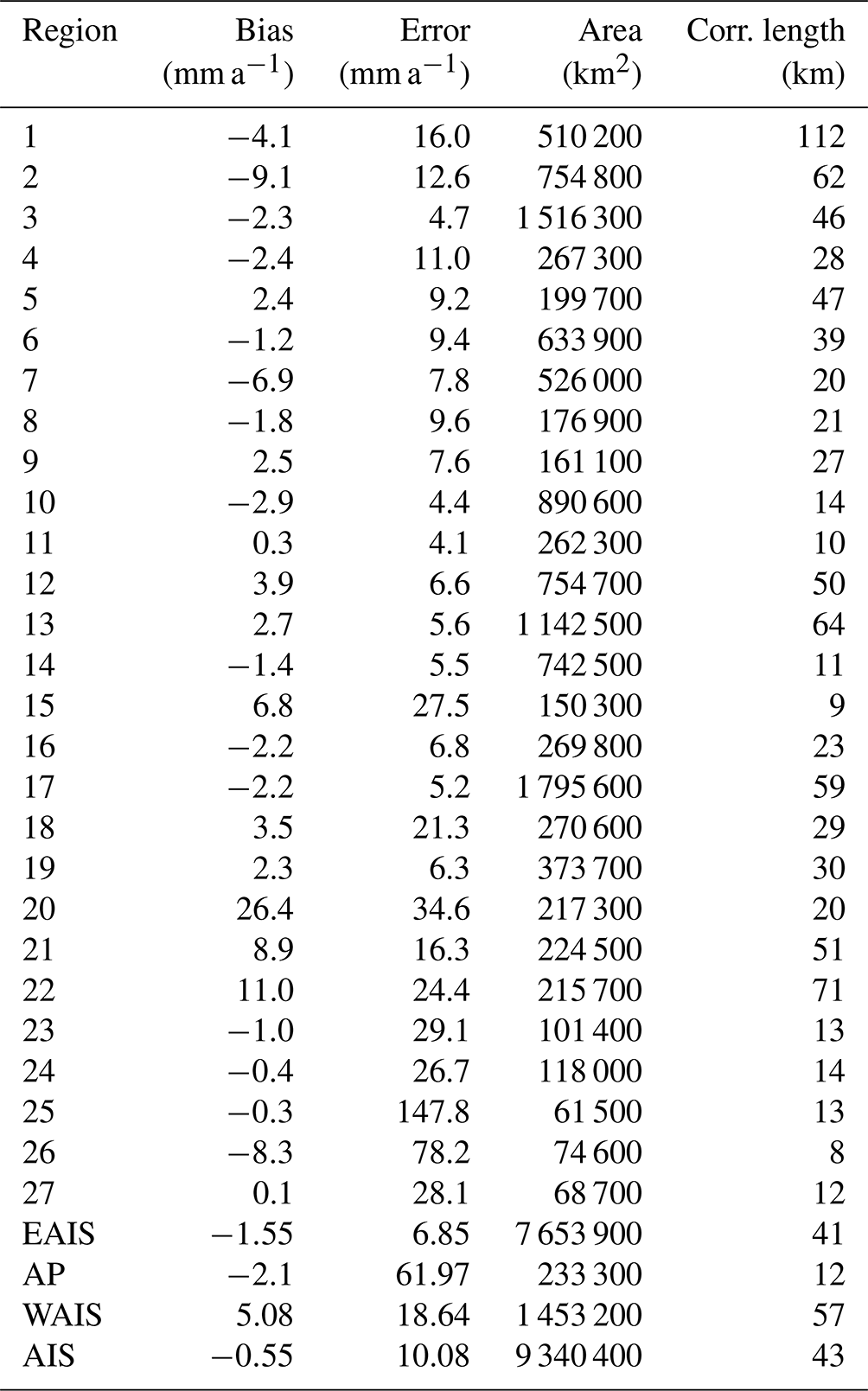
Area integrated error for each drainage region, based on the outlines from Zwally et al. (2012) (shown in Fig. 1), are estimated loosely following the approach of Nilsson et al. (2016). The total area integrated error is divided into three main components: the systematic bias, the random error, and the rate error estimated in the fitting procedure. These are then combined in quadrature to produce the total error according to
where σs is the systematic bias, σr the random error, the rate error, n the number of uncorrelated elevation change estimates (see below), and k the degrees of freedom in the least-squares model (k=2). The systematic bias and the random error are taken as the average and standard deviation of the difference in rate between the Jet Propulsion Laboratory (JPL; this study) and ICESat and ICESat-2 (Smith et al., 2020) products for the 2003–2019 period. We compute the error in the estimated rate using the variance–covariance matrix in the least square fitting procedure according to
where is the average monthly uncertainty from our product inside the time interval of interest, X is the design matrix of the linear model, XT is the transpose of the design matrix, “diag” is the diagonal elements of the array, and −1 is the inverse of the dot products. The subscript is the location of the rate error in the diagonal array. To account for spatial autocorrelation σr and are divided by n; n is estimated by dividing the total area of each drainage region with the correlation area: , where A is the area of the region, and ρ is the correlation length. The errors for each drainage region are summarized in Table 2. The intrinsic quality of each mission was determined through internal crossover analysis (Sect. 4.1) of each mode and mission and is summarized in Table 1 and Fig. 6. Analyzing the correlation length of the laser-only versus JPL elevation change differences we find an ice-sheet-wide correlation length scale on the order of 20–100 km. To be conservative, a correlation length of 100 km was used to compute n.
Table 2Regionally averaged errors for the synthesized JPL record of elevation change, computed relative to the unbiased ICESat to ICESat-2 estimate of Smith et al. (2020). Errors were determined by differencing 2003–2019 linear rates of elevation change between products. The bias (mean: σs) and error (standard deviation: σr) are computed for each drainage basin (1–27; Fig. 1). Antarctic Ice Sheet (AIS), Antarctic Peninsula (AP), West Antarctic Ice Sheet (WAIS), and East Antarctic Ice Sheet (EAIS) statistics are determined using area weighted averages.
5.1 Accuracy of synthesis
Previous studies have relied on near-coincident airborne measurements to validate land ice elevation changes derived from multi-mission synthesis (McMillan et al., 2014; Nilsson et al., 2016; Simonsen and Sørensen, 2017; Wouters et al., 2015). This approach, however, is limited in both the spatial and temporal coverage. For Antarctica, airborne validation data have been collected during austral summer, mostly over rapidly thinning glaciers, such as Pine Island and Thwaites, in the western part of the ice sheet, with significant spatial coverage starting in 2002. The derived errors from these local comparisons are then extrapolated to the entire ice sheet into regions exhibiting very different surface and metrological conditions. With the launch of ICESat-2 in September 2018 we now have, for the first time, the ability to compare long-term unbiased laser-derived rates of elevation change on a continental scale. For this analysis we compare our synthesized rates of elevation change to those estimated by Smith et al. (2020) for the period 2003–2019 for each basin (Zwally et al., 2012) (Fig. 1). The results of this analysis are summarized in Table 2. We find an ice-sheet-wide error of mm a−1 (Fig. 7e) with a quadratic and linear increase as a function of surface slope in the systematic bias and random error, respectively (Fig. 7f and g). To determine the validity of this comparison we also compared ICESat and ICESat-2 rates with rates from ATM over the time period 2003–2018. Good agreement was found between the two datasets with an average difference of 2.3±22 cm a−1 (Fig. 7c) over regions with an observed rate of elevation change from ATM ranging from −15 to 2 m a−1. The main discrepancies between our product and the ICESat- and ICESat-2-derived elevation change are concentrated over areas of high relief and over regions with large magnitude changes, such as Pine Island and Thwaites glaciers (Fig. 7a). Here, differences larger than 10 cm a−1 can be found, and for the main trunk of Pine Island Glacier we find a difference of 2±10 cm a−1 (Fig. 7a). The magnitude of the ATM error compared to the ICESat and ICESat-2 product is larger. This is mostly due to the fact that the data comparison locations are in areas of rapid change. The correlation between the two laser datasets and our product is greater than 0.8 in both cases.
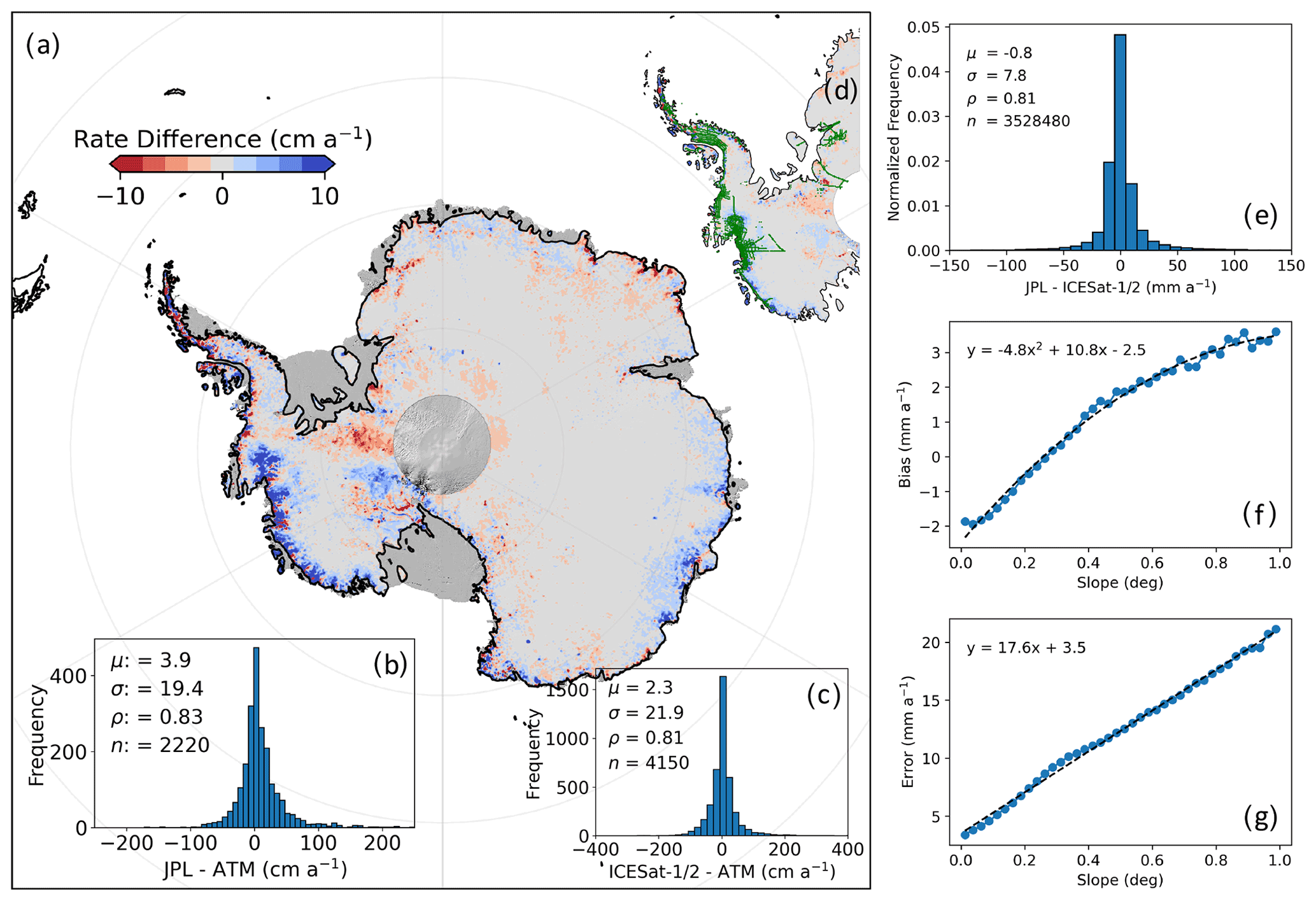
Figure 7Elevation change validation and comparison using rates derived from ICESat and ICESat-2 and airborne ATM data over the time period of 2003–2019 and 2001–2019, respectively. Panel (a) shows the spatial distribution of the elevation change differences from this study (JPL) differenced with rates derived from Smith et al. (2020). Panel (b) shows the comparison of rates derived from JPL with ATM at locations indicated in (d) with green flight lines. Panel (c) shows the comparison between ICESat- and ICESat-2-derived rates with ATM. Panel (e) depicts the ice-sheet-wide histogram of elevation change differences. Panels (b), (c), and (e) include the distribution mean (μ), standard deviation (σ), correlation (ρ), and number of observations (n). Panels (f) and (g) are the bias (mean) and error (standard deviation) as a function of surface slope for the JPL and ICESAT-1 and ICESat-2 validation.
The relative precision of the different satellite altimeters used in this study range from 5 to 40 cm over low slope surfaces (Table 1 and Fig. 6). Earlier missions such as Geosat, ERS-1, and ERS-2 are roughly 3 times less precise than later missions (Envisat, ICESat, ICESat-2, and CryoSat-2). However, it was also found that the ERS-1 and ERS-2 Ocean mode was ∼ 30 % more precise than ice mode data, bringing it closely in line with the later missions. Unfortunately, the data coverage of the ocean mode is far lower than the ice mode. For CryoSat-2, the lower relative precision of the SARIn mode can be attributed to the spatial coverage, with SARIn operating over rougher terrain compared to the LRM mode that operates over the interior of the ice sheet with a higher along-track resolution (i.e., smaller footprint). Similar effects were also seen in Schröder et al. (2019). The laser altimetry missions show the lowest noise levels, on the order of 5 cm over flat areas ranging up to 20 cm for slopes <0.8∘, with ICESat-2 showing a factor-of-2 improvement in precision over its predecessor (ICESat) over all surface slopes.
5.2 Comparison to other studies and datasets
Previous long-term Antarctic Ice Sheet elevation change products have been produced by Dresden University of Technology (TUD; Schröder et al., 2019) and the Centre for Polar Observation and Modelling (CPOM; Shepherd et al., 2019). These products vary in both resolution and processing methodologies. The TUD product is provided at a spatial resolution of 10 km and as monthly elevation change estimates. In contrast, the CPOM product provides elevation change estimates every 5 years at 5 km resolution and basin-wide time series of mass change at quarterly resolution. The TUD dataset is comprised of Seasat, Geosat, ERS-1, ERS-2, Envisat, and CryoSat-2, while CPOM consists of data from ERS-1, ERS-2, Envisat, and CryoSat-2. To allow for a fair comparison between the different products we used our provided product without hypsometric extrapolation for the analysis.
The errors reported for our elevation change synthesis are slightly larger than those reported by TUD; this is due to the difference in retracking and the fitting procedure used to derive the error estimates. Comparing all three data products to the ATM validation data we find the best agreement with the JPL synthesis. (JPL 4±19 cm a−1, TUD 6±20, and CPOM to cm a−1). The JPL and TUD estimates were computed from the same ATM dataset and given the same editing criteria, while values from CPOM are the reported values from Shepherd et al. (2019). Applying the same analysis to the 2007–2011 and 2011–2016 elevation change solutions provided by CPOM, we found values of 29±41 cm a−1 (2007–2011) and cm a−1 (2011–2016) for the comparison with ATM, as well as a weighted average of cm a−1 comparing data from overlapping locations. To further compare the noise level in the different datasets we use the elevation change from the common 1992–2016 time period (as CPOM only provides rates in 5-year intervals) of all products and compare against ICESat and ICESat-2 elevation change rate from 2003 to 2019. To reduce the impact of differences in time span, we initially compare only data between 81.5 and 90∘ S (pole hole) as this spatial domain only contains ICESat and CryoSat-2 measurements and is thus the most closely aligned in time with the ICESat and ICESat-2 estimate. We also perform an ice-sheet-wide analysis, though the time spans are not identical. To compute the noise level, we simply differenced the three rate fields with the ICESat- and ICESat-2-derived rates and computed the average and standard deviation of the differences. This provided the following ice-sheet-wide results: (JPL), (TUD), and cm a−1 (CPOM). For the pole-hole region, 81.5 and 86∘ S, the following results were obtained: (JPL), (TUD), and cm a−1 (CPOM).
Comparing the long-term rates for the overlapping time period 1992–2016, we find an overall good agreement for the three original products. Comparing only values north of 81.5∘ S, we determine volume change rates of −58, −48, and −59 km3 a−1 for JPL, TUD, and CPOM, respectively. Differences are well within the errors for all the three products. Studying the differences in spatial patterns (Fig. 8), using the JPL-derived rate as the reference, we find that the TUD and JPL products agree well over East Antarctica in basins 10–17, while a larger difference can be seen in basin 3 closer to the Weddell Sea. Larger differences between JPL and CPOM compared to JPL versus TUD can be observed in East Antarctica (East Antarctic Ice Sheet: EAIS). This is likely a result of different methodologies for correcting changes in the radar scattering. Dividing the estimates into different regions we find the following volume change estimates for the 1992–2017 period: WAIS (West Antarctic Ice Sheet; JPL −108, TUD −100, and CPOM −106 km3 a−1), EAIS (JPL 61, TUD 48, and CPOM 43 km3 a−1), and AP (JPL −11, TUD 4, and CPOM 5 km3 a−1). The regional estimates agree well among products, with the largest discrepancies found in the Antarctic Peninsula. Here, both the TUD and CPOM products provide a positive volume change compared to the JPL product, highlighting the challenge in obtaining accurate estimates from this region. Comparing the JPL and TUD products with rates from Smith et al. (2020) (ICESat and ICESat-2) over the time period 2003–2017 (again using the original JPL product with no hypsometric extrapolation), we find that the two products agree well over WAIS (JPL −165, TUD −164, and LA −200 km3 a−1) but lower in magnitude compared to ICESat and ICESat-2 due to the larger radar footprint. For EAIS (JPL 83, TUD 51, and LA 85 km3 a−1) a disagreement of roughly 40 % is observed between the TUD and JPL products, in which LA and JPL values are practically identical. In the AP (JPL −19, TUD −7, and LA −39 km3 a−1) both products are lower in magnitude compared to ICESat and ICESat-2, on the order of 50 %–80 % due to limitations in measuring over high relief topography.
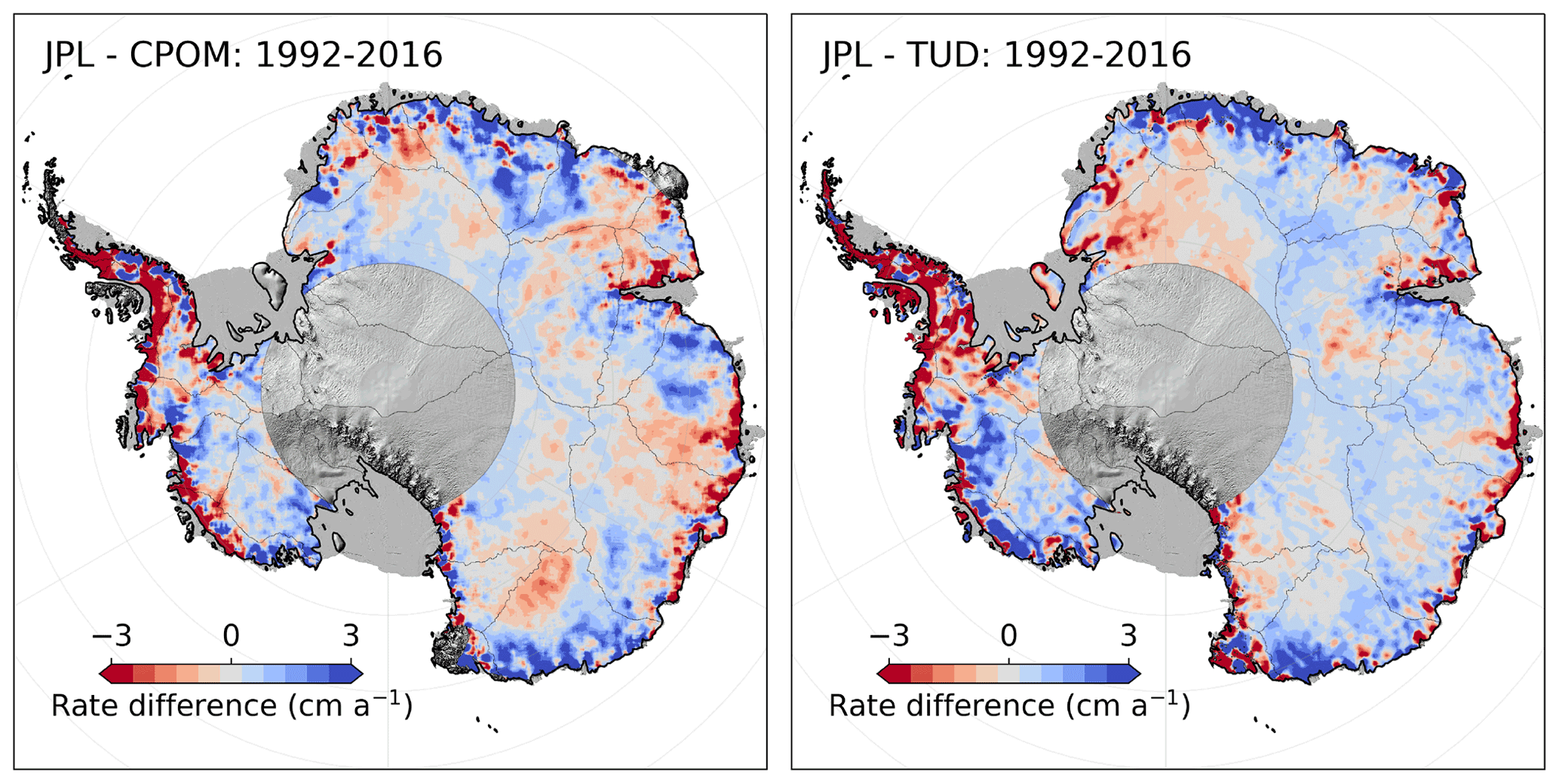
Figure 8Comparison of overlapping long-term rates from the Technical University of Dresden (TUD) and Center for Polar Observation and Modelling (CPOM) altimetry product with rates from this study (JPL).
To understand how well these products can capture (and provide insight into) the change or variability in physical processes of the ice sheets, we compared our result with modeled changes in surface elevations (“zs”) from the IMAU (Institute for Marine and Atmospheric research Utrecht) firn densification model (FDM; Ligtenberg et al., 2012) that is forced by 6 h mass balance components (snowfall, rain, sublimation, and snowmelt), average surface temperature, and 10 m wind speed from the Regional Atmospheric Climate Model version 2.3p2 (van Wessem et al., 2018). The firn model only simulates changes in surface elevation due to changes in surface processes and does not account for thinning or thickening resulting from changes in ice dynamics (flow). To minimize dynamic signals, we mask areas with surface velocities larger than 30 m a−1 using the velocity field provided by the ITS_LIVE project (Gardner et al., 2019) merged with phase-based estimates (Mouginot et al., 2019). The surface elevation long-term trend and acceleration fields (1992–2016), seen in Fig. 9, show that for Dronning Maud Land and Enderby Land (basins 4–11) there is generally good agreement in both the spatial pattern and the sign of the observed and modeled rate of elevation change. For these regions, the observed change can be attributed to an increase in accumulation (Boening et al., 2012). However, the magnitude between the modeled and measured rates of change differs by roughly 50 %. The altimetry-derived volume change for basins 4–11, over the time period 1992–2016, is estimated at 46 km3 a−1 compared to a modeled change of 27 km3 a−1. This disagreement becomes even more prominent for Wilkes Land (basins 12–14) where the difference between modeled and observed rates of change are larger and of opposite signs (Fig. 9). For these three basins, the estimated difference in volume change is on the order of 36 km3 a−1 based on the difference in the modeled change of −25 km3 a−1 compared to 11 km3 a−1 from altimetry. The magnitude and sign of these results are consistent within all three altimetry products compared to the FDM. Further, comparing the differences in the magnitude of the seasonal amplitude for 1992–2016, we find that the TUD product has an annual amplitude that is ∼50 % larger than the JPL product (5.1±15 versus 2.7±4.9 cm). Our estimated value of 2.7±4.9 cm compares well with the 2.9±4.1 cm average FDM amplitude for the period 1992–2016. This analysis was not applied to the CPOM product as their provided basin time series are in units of mass after a firn correction has been applied.
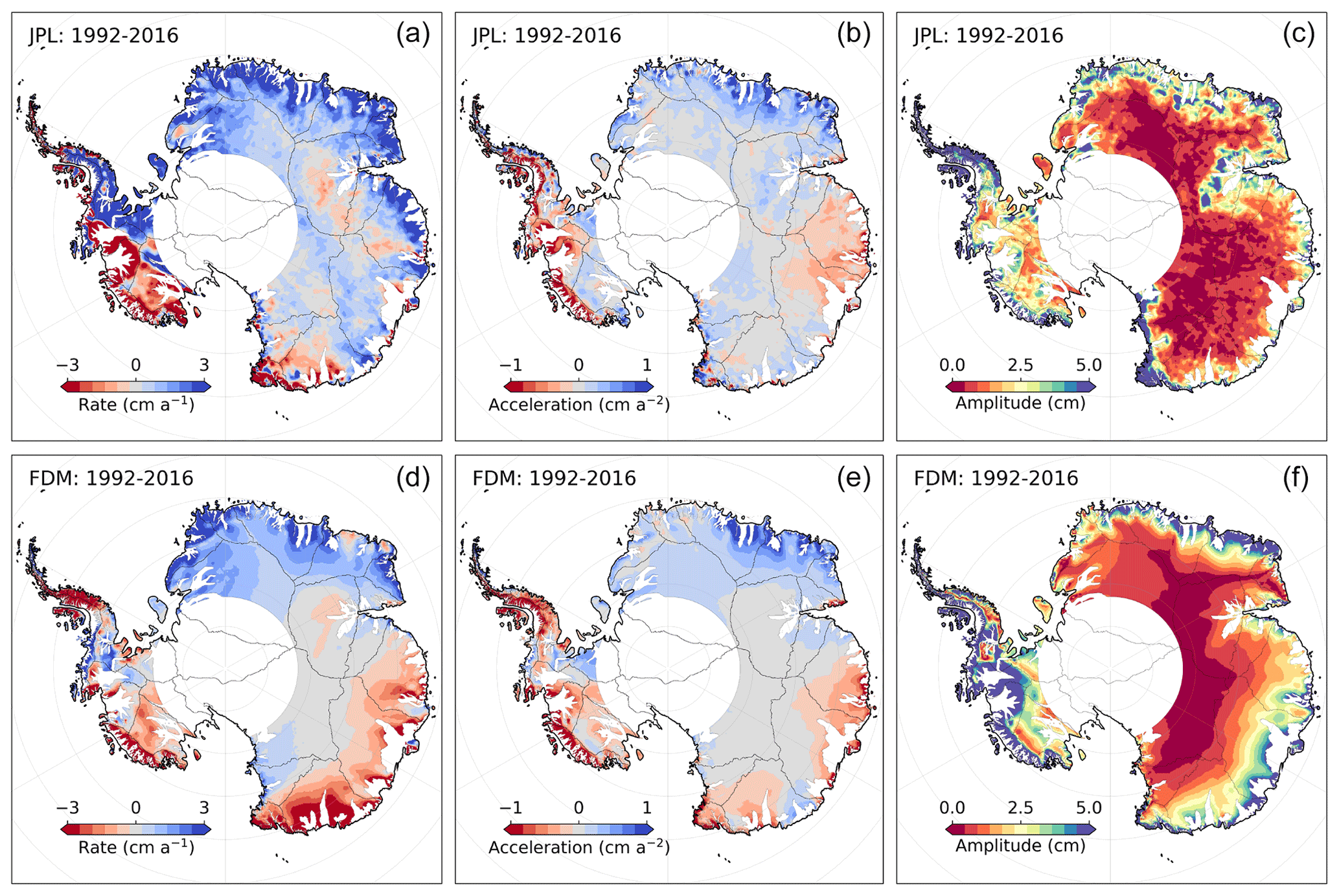
Figure 9Spatial fields of rates (a, d), acceleration (b, e) and seasonal amplitudes (c, f) from our product (JPL; a–c) and modeled values from the IMAU firn densification model (FDM; d–f). Areas of fast flow (>30 m a−1) have been masked out to minimize height changes caused by changes in ice flow. The altimetry data has been smoothed with a 50 km median filter to highlight large-scale spatial patterns.
5.3 Basin-scale time-evolving volume change
Analyzing the 1992–2020 record of surface elevation (Table 3 and Figs. 10 and 11), including the area between 81.5 and 90∘ S, we determine an average rate of volume change of km3 a−1 over the entire ice sheet, with large losses from the West Antarctic Ice Sheet ( km3 a−1) and gains for East Antarctic Ice Sheet ( km3 a−1) which experienced large snowfall events in 2009 and 2011 (Boening et al., 2012). The Antarctic Peninsula (AP) is the most challenging region to measure elevation change due to its extreme surface relief and sparse data coverage. We anticipate that any estimate derived from conventional satellite radar altimetry will be biased positive due to the inability to measure low-elevation signals. That said, we estimate an overall negative trend for the AP of km3 a−1 for the 29-year record (1992–2020) (Figs. 10 and 11), which aligns closely with other estimates (Groh el al., 2021; Rignot et al., 2019; The IMBIE team, 2018; Zwally et al., 2021) but is highly dependent on the applied hypsometric extrapolation (Sect. 3.2.5). On decadal timescales we find that the large glaciers systems of Pine Island, Thwaites, Smith, and Kohler (basins 21 and 22) have shown relatively stable mass loss since the early parts of the satellite era, with signs of accelerated thinning since 2007–2009 (Fig. 11). WAIS has seen almost a doubling of its mass loss in the last decade (2011–2020) compared to the two previous decades (Fig. 11). EAIS has reverted back to its previous long-term decadal rate of ∼ +8 km3 a−1, in line with the observed 5-year trend from Geosat over Dronning Maud Land (Figs. 11 and 12), down from +84 km3 a−1 following the anomalous snowfall during the 2001–2011 period. AP was in balance and saw little observable change in the first decade (1991–2010) but increased its mass loss by a factor of 10 in the period of 2001–2011. The mass loss in the last decade was slowed by roughly 50 % due to a positive mass balance anomaly during the period 2016–2018. Over the Geosat time period from 1985 to 1989, and for latitudes <72∘ S, a general stable and small positive rate of 6±16 km3 a−1 was found for the EA1 region (basins 4–11; Fig. 12). This rate remained stable between 1985 and 2009 (∼ 10 km3 a−1) until the onset of a precipitation event in 2009. For the EA2 region (basins 12–15; Fig. 1) a shift in both sign and magnitude was observed for the 1985–1989 period compared to the long-term positive rate for EA1. The mass loss over the 1985–1989 period was km3 a−1 and was found to be mostly driven by the Totten Glacier system in basin 13 (Fig. 10). This rate is based, however, on heavy extrapolation over the Totten region due to poor data coverage for the last 2 years of the mission and should be treated with caution. Trends for EA2 showed a stable negative rate (∼ 25–30 km3 a−1) until 2001–2003 when a large positive change occurred due to an increase in SMB (surface mass balance; Fig. 10c). The region reverted back to a long-term negative trend after 2006 mostly modulated by changes in SMB.
Table 3Volume change rates spanning 1985 to 2020 for basins 1–27 (Fig. 1) and aggregate regions. Volume change errors are computed from the ICESat and ICESat-2 validation procedure, combined with the error in the estimated rate.
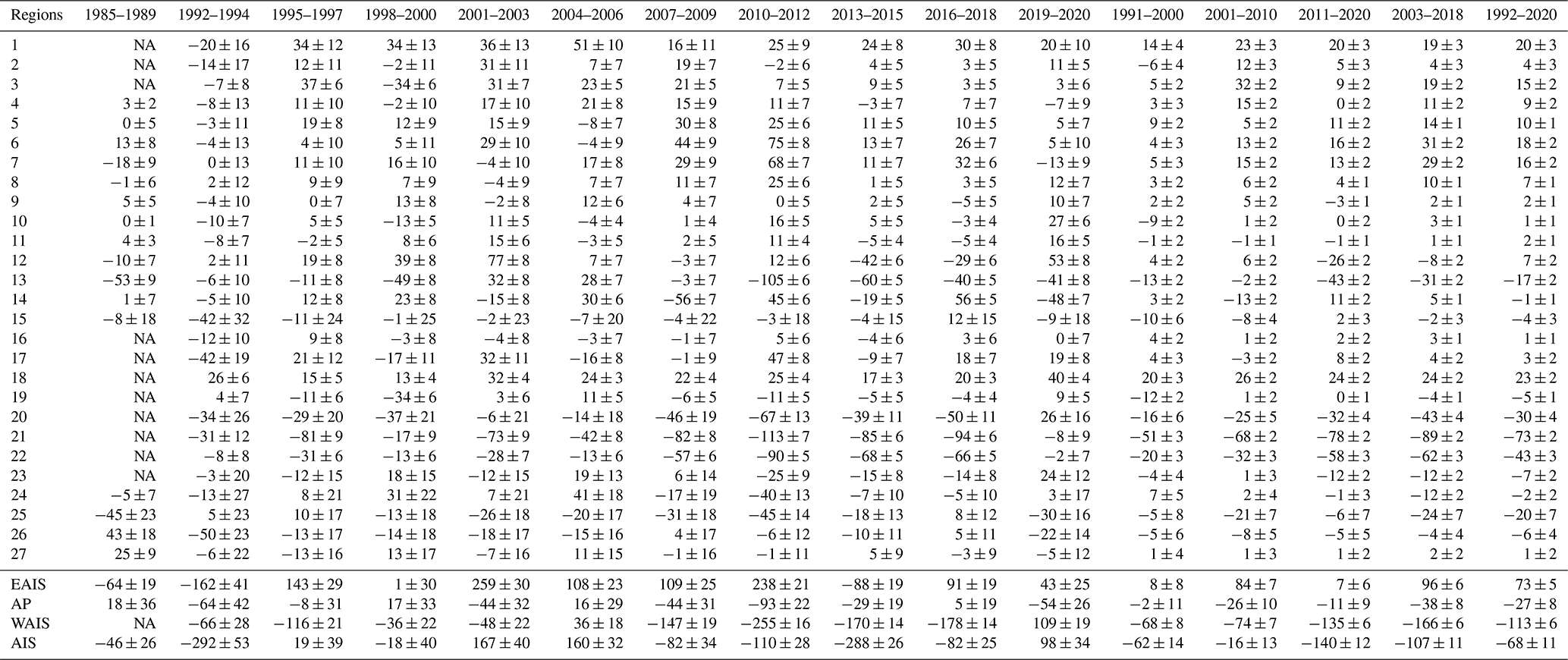
NA: not available
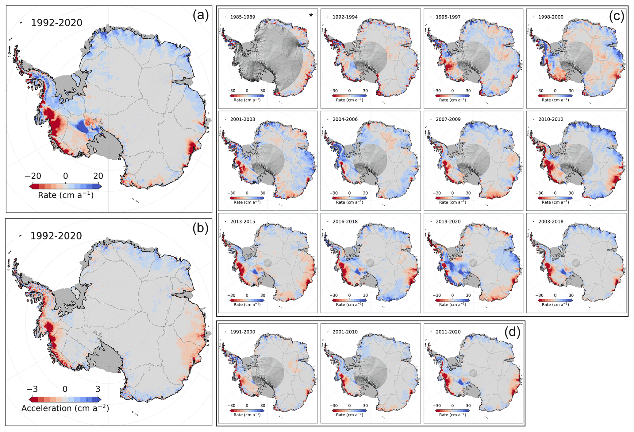
Figure 10Rates of Antarctic Ice Sheet elevation change. Elevation change rate (a) and acceleration (b) for the 1992–2020 period and average rates for (c) 3-year, (d) ICESat and ICESat-2, and (d) 10-year intervals. The * indicates a 5-year interval for Geosat.
Regionally, concentrated rates of thinning from accelerated glacier flow (Gardner et al., 2018; Rignot et al., 2019) are found to spread inland over time due to a regional dynamic imbalance (Shepherd et al., 2019). The marginal areas surrounding the Getz Ice Shelf (basin 20) also exhibit negative rates of elevation change but are more localized to the narrow glacier outlets due to inland topographic barriers and time since initiation of thinning (Figs. 10 and 11). This area saw a large break in the overall long-term trend around 2010 when rapid onset thinning was observed and attributed to short-term variations in both the surface mass balance and ice dynamics (Chuter et al., 2017; Schröder et al., 2019; Gardner et al., 2018). Basin 18, which contains the Kamb Ice Stream, experienced a relatively steady gain in volume over the last three decades resulting from the stagnation of the Kamb Ice Stream some 200 years prior (Catania et al., 2006) (Figs. 10 and 11). Totten Glacier (basin 13), part of the EAIS, has been losing mass since the late 1970s (Schröder et al., 2019) with the average trend mostly governed by ice dynamics and short-term variability and acceleration driven by changes in precipitation (Li et al., 2016). A major change in trend was observed in 2010 when a large-scale thinning of the entire glacier is observed, likely in response to a change in precipitation and possibly changes in ice dynamics driven by changes in ocean conditions (Khazendar et al., 2013; Li et al., 2016). The activation or reversal in trend of both the Totten and Denman glaciers in early 2009–2010 has disrupted the long-term equilibrium or gain that has been observed for most parts of Wilkes Land (basins 12 and 13; Fig. 1). A departure from the long-term trend can now be observed for large parts of Wilkes Land in the form of large-scale negative acceleration spreading inland (Fig. 10). In Dronning Maud Land and Enderby Land (basins 5–8), the previously mentioned snowfall events in 2009 and 2011 (Boening et al., 2012) are clearly observed in the regional elevation change trends. This pattern is most prominent along the Weddell Sea coast where the accumulation signal, in the form of precipitation, shows an earlier event in 2006 (basins 3 and 4) (Figs. 10 and 11). The glaciers flowing into the Bellingshausen Sea have shown a complex pattern of change over the last 29 years. Here, Palmer Land (basin 24) shows a steady increase in surface elevation over the initial 15 years of the record, following a long-term positive anomaly in precipitation from 1992. However, a reversal in this pattern was observed around 2007 when patterns of thinning (McMillan et al., 2014; Schröder et al., 2019; Shepherd et al., 2019; Wouters et al., 2015) (Fig. 10) can be observed localized to the major low-elevation outlet glaciers in the regions. The change can be largely attributed to a change in precipitation amount, with lesser contributions from changes in ice dynamics resulting from enhanced melting by the ocean (Gardner et al., 2018; Hogg et al., 2017). However, in the southern part of the Bellingshausen Sea, near Ferrigno Glacier in basin 23, we find a relatively stable trend during most of the record until 2009 when a large acceleration in ice loss can be observed. This acceleration can only be partially attributed to changes in ice dynamics (Gardner et al., 2018; Wouters et al., 2015), and it is likely that changes in precipitation are the major driver of change. Large changes in both spatial and temporal variability can be observed in the AP region in the last three decades, when large-scale reversals of signals can be observed over different time periods. Here, we find a large-scale positive elevation change anomaly in basins 23–26, superimposed on a long-term negative trend, over the time periods 1998–2000, 2004–2006, and 2016–2018. These changes are linked to changes in the short-term variability in SMB in the region due to increased precipitation. Examining the rates derived over the ICESat-2 time period (2018–2020) a large positive elevation change signal can be observed over the WAIS region, in contrast to the overall negative long-term trend. This anomaly is directly linked to large-scale snow accumulation resulting from an extreme precipitation event in the austral winter of 2019 which has been attributed to the landfall of atmospheric rivers (Adusumilli et al., 2021).
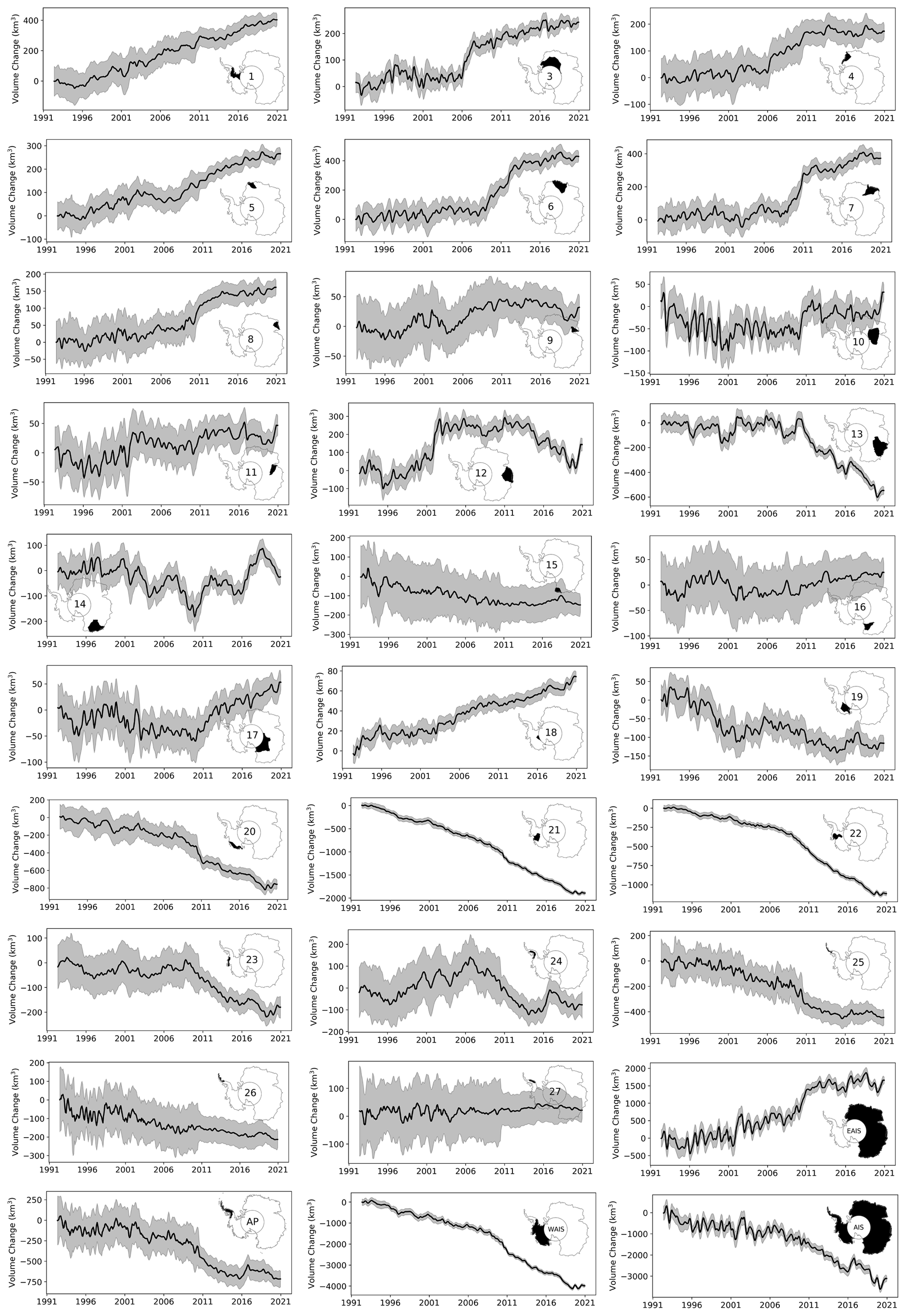
Figure 11Basin (Zwally et al., 2012) and ice sheet monthly elevation change time series for the period of 1992 to 2020.
We provide a new elevation change product for the Antarctic Ice Sheet that synthesizes over three decades of data from seven different satellite altimeters. To do this we applied slope corrections to all pulse-limited radar altimetry datasets, substantially reducing the overall error in both measured elevation and elevation change rates as can be seen in the crossover quality analysis. Our methodology explicitly separates the time-variable and the static topography in the inversion for elevation change and is one of the major improvements over previous studies (Flament and Rémy, 2012; McMillan et al., 2014; Moholdt et al., 2010). Removing the time-invariant topography from the time-variable elevation allowed us to more easily accommodate varying spatial scales of correlation inherent to the different processes affecting the altimetry retrievals of elevation. This can be conceptualized by noting that correlation lengths are less than 10 km for the time-invariant topography, while elevation change signals are correlated at length scales greater than 50 km in some places. We performed extensive testing over Lake Vostok in East Antarctica and concluded that the optimum search radius for estimating time-invariant topography was 500 m for repeat-track missions and 1000 m for drifting-track missions. An extensive investigation was also undertaken to determine the optimum radius for maximizing correlation between the waveform parameters and the time-variable elevation change. From this analysis it was determined that a 1000 m search radius provided the best results in both minimizing the trend and RMS of the residuals. Both spatial and temporal patterns of changes in the scattering horizon (penetration depth) (Figs. 2 and 3) of the radar signal further highlight the importance of this correction, which can reach magnitudes of several centimeters per year (Fig. 3). This correction also has a significant impact on the magnitude of the seasonal signal at continent-wide scales and can produce reductions of upwards of 50 % in the seasonal amplitude of the elevation change signal (Figs. 3 and 5).
Cross-calibration of the different missions is likely the most challenging barrier to generating a continuous and accurate record of elevation change. In this study we have taken a somewhat different approach to Schröder et al. (2019) and Shepherd et al. (2019). Here, we work entirely in residual space after the removal of time-invariant topography. We first apply a least-squares approach to provide an initial intermission adjustment. This adjustment is mainly to align overlapping data and modes such as ICESat and Envisat. The approach also has advantages of removing long-term trends and seasonality, allowing us to estimate any remaining offset by examining the residuals to the least-squares model. We find here that the Envisat and CryoSat-2 transition is troublesome as only a few months of data overlap exist due to the later change in orbit of the Envisat mission and the large ice-sheet-wide changes that occur around this transition. To overcome the sampling problem and the variable elevation change behavior observed for different locations, we investigated several methods to estimate Envisat and CryoSat-2 offsets. Given the availability of high-accuracy ICESat and ICESat-2 elevation change rates we were able to determine which offset provided the most appropriate trend compared to the laser altimetry reference. One should note that we do not use the laser altimetry data to scale or generate the offset; its merely an independent guide to select the most suitable offset produced from the different alignment approaches. This method provides volume changes that are well in line with both the CPOM and TUD products, which provides us with confidence in our approach. Further, it is unfortunate that Envisat changed orbit in late 2010 as it would have allowed almost 2 years of overlap with CryoSat-2. Hopefully these data can be included in the future versions once the issue of how to satisfactorily handle the change in orbit can be addressed. This work is currently being undertaken. As of now, including post-orbit-change data in the synthesis has the effect of introducing noise in the Envisat time series and spurious offsets, severely limiting the use of the data. For the Geosat data we include a caveat for the quality of the cross-calibration. A cross-calibration has been applied, but the quality of this adjustment can vary due to the long gap separation between Geosat (ending in 1990) and the next altimetry mission (ERS-1, starting in 1992). We recommend that care be taken here and suggest that for regional studies a manual post-calibration be applied. The suggestion would be to follow the approach outlined in Sect. 3.2.3 using Eq. (2) varying the degree of the polynomial until satisfactory results are obtained, as seen in Fig. 12.

Figure 12Monthly elevation change time series for the area measured by Geosat (72∘ S latitude limit) for the period 1985–2020. The large difference in RMS seen in the Geosat time series for the full ice sheet is mostly driven by observations collected over the Antarctic Peninsula. The regional Geosat time series were recalibrated to allow for better alignment with the long-term record, as suggested in Sect. 6. This as the local offset estimated at each grid cell for Geosat might not be of sufficient quality everywhere.
Another important altimetry correction in the processing is the amplitude normalization, using CryoSat-2 as a reference. Figure 5 illustrates that even after applying corrections for the change in scattering horizon (e.g., penetration bias), the different missions show inconsistent seasonal amplitudes from the older pulse-limited mission that has seasonal amplitudes that are more than twice that of newer missions (e.g., Envisat, CryoSat-2, ICESat, and ICESat-2). This is most likely linked to the higher level of noise in the older sensors (∼ 30 cm vs. ∼ 10 cm). The larger noise levels make it difficult to separate the change in a shifting scattering horizon with time-invariant topography. Hence, there is a need to normalize the different seasonal amplitudes over the different missions as there is no physical justification for why they should differ. Here we found that both the ICESat and CryoSat-2 missions showed remarkable good agreement in seasonal amplitude with surface elevation change simulated by the RACMO firn densification model (Ligtenberg et al., 2012). In the end we selected CryoSat-2 as the reference as it provides both higher spatial and temporal sampling compared to ICESat. ICESat-2 was not considered as we believe that the record currently is too short (only 2 years were used in this study) to provide a viable estimate of seasonal climatology. It should be noted that this correction removes the mean difference in amplitude between missions but does not modulate the seasonal-phase or the inter-annual variability in the amplitude within a single mission.
Large data gaps exist at latitudes exceeding the maximum orbital coverage; this gap is referred to as the pole hole. In our product we fill the pole hole to provide a spatially complete field to aid in the estimation of ice-sheet-wide mass balance and to make the data more usable for modeling efforts. However, we do recognize that our chosen interpolation method may not be appropriate for regions such as AP and basins 15–17, which are comprised of highly variable topography. Therefore, we provide a mask layer (data_flag) that identifies high-quality, low-quality (high topographic relief), and pole-hole data. After some investigation we found that applying the hypsometry method to extrapolate monthly estimates of elevation change produced an improved estimate of basin-scale volume changes when compared to the ICESat and ICESat-2 product. This methodology is not applied to the distributed product. We leave it up to the user of the product to apply their own methodology for extrapolation, but we recommend the hypsometric method when generating basin-scale mass balance estimates.
Elevation change rates near the pole hole are relatively small due to low precipitation amounts (Wingham et al., 2006) and few dynamically active glaciers. Changes in mass within the pole hole only amount to few tens of gigatons of change (Shepherd et al., 2019), once corrected for firn air content. Hence, the interpolation of data to fill the pole hole only contributes a small part of the overall volume change. In our estimate the overall volume change is estimated to be 26 km3 a−1 south of 81.5∘ S over the full 2003–2018 time period using the least-squares adjustment method and 34 km3 a−1 when adding the residual cross-calibration. This aligns well with the value estimated from the ICESat and ICESat-2 product of 37 km3 a−1 for the area 81.5–86∘ S over the period 2003–2019. Studying the other two publicly available altimetry syntheses we find that their pole-hole volume estimates are biased in the negative direction (compared to the ICESat and ICESat-2 product) and can be quite large: −65 (CPOM) and −12 km3 a−1 (TUD). This indicates that using either a constant offset or mission-only derived trends for cross-calibration might not be sufficient for these areas as a small error can a have a large impact when integrated over a large region. This further points to the effectiveness of using the least-squares adjustment for cross-calibrating non-overlapping records.
Previous altimetry studies of Antarctic mass balance have relied heavily on airborne laser altimetry to provide validation and estimates of the overall volume change uncertainty (McMillan et al., 2014; Wouters et al., 2015). However, airborne data are both limited in spatial and temporal coverage, making it extremely difficult to estimate volume change uncertainties on continental scales. We, for the first time, have used long-term (16-year) unbiased laser-altimetry-derived rates of elevation change from Smith et al. (2020) to produce ice-sheet-wide uncertainties for our product. This is especially important for East Antarctica where a very small amount of validation data exist from either in situ or airborne campaigns. Though the rates here are on the order of centimeters per year, they occur over massive spatial scales and contribute significantly to the overall ice sheet volume change. A total of 16 years of high-accuracy laser data allows us to validate these centimeter trends as the measurement error reduces as a function of time. This dataset allows us to quantify and validate changes at the millimeter per year level, which was previously not possible in East Antarctica. The overall uncertainty estimates of mm a−1 is heavily dominated by the small difference in the interior areas of the ice sheet, which rapidly increase closer to the coast with errors reaching 25 mm a−1. In general, the analysis shows that radar altimeters underperform, relative to laser altimeters, in areas of steep topography where change signals are largest. Further, we observe that in East Antarctica, the radar record in many places produces small negative rates, compared to slightly positive rates from lasers, indicating residual issues with time-variable radar penetration biases. These issues are of course known to the scientific community (Arthern et al., 2001; Davis, 1993; Lacroix et al., 2009; Legresy and Remy, 1997; Nilsson et al., 2015b), and they are an area of active research. However, with this new laser altimetry dataset we now have at least the possibility of quantifying this type of uncertainty across nearly the entirety of the ice sheet.
Comparing the estimate from this study with the TUD (Schröder et al., 2019) and CPOM (Shepherd et al., 2019) products, we find good agreement over the 1992–2016 time period, with differences within the error budgets of the respective products. This agreement is a good indicator that all three products provide consistent results given the different processing methodologies for areas below 81.5∘ S. Analyzing further, we find that the main difference between products is in the overall noise levels. Given the different comparisons we find that, on average, our product has lower noise and agrees most closely with the laser altimetry validation data. We attribute this improvement in noise characteristics to the improved processing techniques.
Another important improvement is the normalization of the seasonal signal across missions. Though this correction is not perfect, it has lowered the magnitude of the average seasonal signal to a level comparable to the simulated values of elevation change from the RACMO FDM product (Ligtenberg et al., 2012). Accurate quantification of the “seasonal breathing” of the Antarctic Ice Sheet is an important component to estimated rates of snowfall. However, we do find a discrepancy between the altimetric and modeled rates of change for East Antarctica, with rates of change differing in places by 200 % to 300 % for the 1992–2016 period. We further find that the direction of change can have the opposite sign between modeled and observed rates, as can be seen in the Wilkes Land region. This indicates that the current generation of firn densification models, though highly successful in representing the main components governing ice sheet mass balance, still cannot fully capture all the complex interactions driving changes in surface elevation. This of course has large implications for estimating the East Antarctica mass balance as the correction for firn air content can be as large as 100 % of the measured altimetry signal in some basins (Smith et al., 2020). However, several new firn models are expected to become available within the near future which will greatly help the community to quantify both the error in these models and to help improve our understanding of the processes driving the ice sheet mass balance.
Data can be found in Nilsson et al. (2021), https://doi.org/10.5067/L3LSVDZS15ZV. The code and algorithm used to generate the product are part of the “Cryosphere Altimetry Processing Toolkit” (captoolkit) and can be found here: https://github.com/nasa-jpl/captoolkit (last access: 4 May 2022) and https://doi.org/10.5281/zenodo.3665785 (Paolo et al. 2020).
In this study we have provided a 36-year record (1985–2020) of elevation change for the Antarctic Ice Sheet derived from seven altimetry missions combining both laser and radar measurements. Elevation changes were derived from measurements of surface elevation by first removing the time-invariant topography for each mission and applying corrections for varying surface scattering characteristics that affect radar altimetry. The different sensors and modes were cross-calibrated and merged into a continuous record of elevation change using a combination of interpolation and extrapolation techniques to construct a consistent spatiotemporal dataset for the scientific community.
Our dataset indicates that between 1992 and the later parts of the 2000s, the Antarctic Ice Sheet was in near balance, with modest EAIS gains equaling WAIS losses. In the later parts of the 2000s accelerated WAIS losses outpaced EAIS gains, leading to significant net decrease in ice sheet volume. This accelerated loss has been attributed to increased ocean melting and changes in precipitation (The IMBIE team, 2018). East Antarctica has also seen changes over the last 30 years, in which large swaths of Wilkes Land have been showing accelerating negative elevation change starting around the year 2010 and likely stemming from changes in precipitation/firn, as well as possibly ice dynamics from the Denman and Totten glacier systems. The Dronning Maud Land region has started to show extensive elevation gain due to significant increases in snowfall beginning around 2009. However, one of the main questions still remains: is EAIS losing or gaining mass? With these long-term improved datasets, in combination with accurate firn modeling, we may soon be able to answer this question. The western parts of Antarctica have seen both consistent and accelerated mass loss over the entire altimetry record dominated by the glacier systems of Pine Island and Thwaites. These areas now show drawdowns for hundreds of kilometers inland and currently show no signs of slowing down. The Antarctic Peninsula also shows signals of major mass loss, but the long-term accuracy of those estimates is hard to quantify due to inherent limitations of radar measurements over these types of rugged terrain. We can, however, say with confidence that large changes due to a complex mix of atmosphere and ocean forcing have accelerated mass loss in the Bellingshausen Sea over the length of the record (Gardner et al., 2018; Hogg et al., 2017; Wouters et al., 2015). This region was relatively stable for two decades but started to show a large change in behavior from its original trend in the 2008–2010 period.
It is our hope that the newly produced ITS_LIVE synthesized record of Antarctic Ice Sheet elevation change will improve understanding of the underlying processes driving the patterns of elevation change with the hope that such understanding will lead to improved projections of ice sheet and sea level change.
The supplement related to this article is available online at: https://doi.org/10.5194/essd-14-3573-2022-supplement.
JN and ASG conceptualized the study. JN conducted the analysis, wrote the majority of the main text, and made all figures. JN, ASG, and FSP all contributed to conceptualization and algorithm development. All authors contributed to the writing and editing of the manuscript.
The contact author has declared that neither they nor their co-authors have any competing interests.
Publisher's note: Copernicus Publications remains neutral with regard to jurisdictional claims in published maps and institutional affiliations.
The authors were supported by the ITS_LIVE project awarded through NASA MEaSUREs program, and the NASA Cryosphere program through participation in the ICESat-2 science team. We thank the NASA and the European Space Agency (ESA) for distributing their radar altimetry data. The author would like to thank Sebastian Bjerregaard Simonsen for the discussions and data support during the early part of the study; it was immensely helpful. We would also like to thank Catherine Walker for producing the altimeter mission timeline inset figure used in Fig. 1. Further, we would also like to thank Ludwig Schröder for his help with obtaining the Geosat data, as well as Veit Helm and the anonymous reviewer for their helpful comments which greatly improved the manuscript. The research described in this paper was carried out at the Jet Propulsion Laboratory, California Institute of Technology, under a contract with NASA.
This research has been supported by the Jet Propulsion Laboratory (NASA MEaSUREs and NASA Cryosphere Science Program (grant no. NNH16ZDA001N-ICESAT2)), as well as the Jet Propulsion Laboratory, California Institute of Technology, through an agreement with the National Aeronautics and Space Administration.
This paper was edited by Ge Peng and reviewed by Veit Helm and one anonymous referee.
Adusumilli, S., Fish, M., Fricker, H. A., and Medley, B.: Atmospheric River Precipitation Contributed to Rapid Increases in Surface Height of the West Antarctic Ice Sheet in 2019, Geophys. Res. Lett., 48, e2020GL091076, https://doi.org/10.1029/2020GL091076, 2021.
Armitage, T. W. K., Wingham, D. J., and Ridout, A. L.: Meteorological Origin of the Static Crossover Pattern Present in Low-Resolution-Mode CryoSat-2 Data Over Central Antarctica, IEEE Geosci. Remote Sens. Lett., 11, 1295–1299, https://doi.org/10.1109/LGRS.2013.2292821, 2014.
Arthern, R., Wingham, D., and Ridout, A.: Controls on ERS altimeter measurements over ice sheets: Footprint-scale topography, backscatter fluctuations, and the dependence of microwave penetration depth on satellite orientation, J. Geophys. Res.-Atmos., 106, 33471–33484, https://doi.org/10.1029/2001JD000498, 2001.
Bamber, J. L.: Ice sheet altimeter processing scheme, Int. J. Remote Sens., 15, 925–938, https://doi.org/10.1080/01431169408954125, 1994.
Bevis, M. and Brown, A.: Trajectory models and reference frames for crustal motion geodesy, J. Geod., 88, 283–311, https://doi.org/10.1007/s00190-013-0685-5, 2014.
Boening, C., Lebsock, M., Landerer, F., and Stephens, G.: Snowfall-driven mass change on the East Antarctic ice sheet, Geophys. Res. Lett., 39, L21501, https://doi.org/10.1029/2012GL053316, 2012.
Borsa, A. A., Moholdt, G., Fricker, H. A., and Brunt, K. M.: A range correction for ICESat and its potential impact on ice-sheet mass balance studies, The Cryosphere, 8, 345–357, https://doi.org/10.5194/tc-8-345-2014, 2014.
Borsa, A. A., Fricker, H. A., and Brunt, K. M.: A Terrestrial Validation of ICESat Elevation Measurements and Implications for Global Reanalyses, IEEE T. Geosci. Remote, 57, 6946–6959, https://doi.org/10.1109/TGRS.2019.2909739, 2019.
Brenner, A. C., Blndschadler, R. A., Thomas, R. H., and Zwally, H. J.: Slope-induced errors in radar altimetry over continental ice sheets, J. Geophys. Res., 88, 1617, https://doi.org/10.1029/JC088iC03p01617, 1983.
Brenner, A. C., DiMarzio, J. P., and Zwally, H. J.: Precision and Accuracy of Satellite Radar and Laser Altimeter Data Over the Continental Ice Sheets, IEEE T. Geosci. Remote, 45, 321–331, https://doi.org/10.1109/TGRS.2006.887172, 2007.
Brockley, D. J., Baker, S., Femenias, P., Martinez, B., Massmann, F. H., Otten, M., Paul, F., Picard, B., Prandi, P., Roca, M., Rudenko, S., Scharroo, R., and Visser, P.: REAPER: Reprocessing 12 Years of ERS-1 and ERS-2 Altimeters and Microwave Radiometer Data, IEEE T. Geosci. Remote, 55, 5506–5514, https://doi.org/10.1109/TGRS.2017.2709343, 2017.
Brunt, K. M., Hawley, R. L., Lutz, E. R., Studinger, M., Sonntag, J. G., Hofton, M. A., Andrews, L. C., and Neumann, T. A.: Assessment of NASA airborne laser altimetry data using ground-based GPS data near Summit Station, Greenland, The Cryosphere, 11, 681–692, https://doi.org/10.5194/tc-11-681-2017, 2017.
Catania, G. A., Scambos, T. A., Conway, H., and Raymond, C. F.: Sequential stagnation of Kamb Ice Stream, West Antarctica, Geophys. Res. Lett., 33, L14502, https://doi.org/10.1029/2006GL026430, 2006.
Chuter, S. J., Martín-Español, A., Wouters, B., and Bamber, J. L.: Mass balance reassessment of glaciers draining into the Abbot and Getz Ice Shelves of West Antarctica, Geophys. Res. Lett., 44, 7328–7337, https://doi.org/10.1002/2017GL073087, 2017.
Davis, C. H.: Surface and volume scattering retracking algorithm for ice sheet satellite altimetry, IEEE T. Geosci. Remote, 31, 811–818, https://doi.org/10.1109/36.239903, 1993.
Davis, C. H.: Snowfall-Driven Growth in East Antarctic Ice Sheet Mitigates Recent Sea-Level Rise, Science, 308, 1898–1901, https://doi.org/10.1126/science.1110662, 2005.
Davis, C. H. and Ferguson, A. C.: Elevation change of the Antarctic ice sheet, 1995–2000, from ERS-2 satellite radar altimetry, IEEE T. Geosci. Remote, 42, 2437–2445, https://doi.org/10.1109/TGRS.2004.836789, 2004.
Davis, J. L., Wernicke, B. P., and Tamisiea, M. E.: On seasonal signals in geodetic time series, J. Geophys. Res.-Sol. Ea., 117, 1–10, https://doi.org/10.1029/2011JB008690, 2012.
Flament, T. and Rémy, F.: Dynamic thinning of Antarctic glaciers from along-track repeat radar altimetry, J. Glaciol., 58, 830–840, https://doi.org/10.3189/2012JoG11J118, 2012.
Fretwell, P., Pritchard, H. D., Vaughan, D. G., Bamber, J. L., Barrand, N. E., Bell, R., Bianchi, C., Bingham, R. G., Blankenship, D. D., Casassa, G., Catania, G., Callens, D., Conway, H., Cook, A. J., Corr, H. F. J., Damaske, D., Damm, V., Ferraccioli, F., Forsberg, R., Fujita, S., Gim, Y., Gogineni, P., Griggs, J. A., Hindmarsh, R. C. A., Holmlund, P., Holt, J. W., Jacobel, R. W., Jenkins, A., Jokat, W., Jordan, T., King, E. C., Kohler, J., Krabill, W., Riger-Kusk, M., Langley, K. A., Leitchenkov, G., Leuschen, C., Luyendyk, B. P., Matsuoka, K., Mouginot, J., Nitsche, F. O., Nogi, Y., Nost, O. A., Popov, S. V., Rignot, E., Rippin, D. M., Rivera, A., Roberts, J., Ross, N., Siegert, M. J., Smith, A. M., Steinhage, D., Studinger, M., Sun, B., Tinto, B. K., Welch, B. C., Wilson, D., Young, D. A., Xiangbin, C., and Zirizzotti, A.: Bedmap2: improved ice bed, surface and thickness datasets for Antarctica, The Cryosphere, 7, 375–393, https://doi.org/10.5194/tc-7-375-2013, 2013.
Gardner, A. S., Moholdt, G., Scambos, T., Fahnstock, M., Ligtenberg, S., van den Broeke, M., and Nilsson, J.: Increased West Antarctic and unchanged East Antarctic ice discharge over the last 7 years, The Cryosphere, 12, 521–547, https://doi.org/10.5194/tc-12-521-2018, 2018.
Gardner, A. S., Fahnestock, M. A., and Scambos, T. A.: ITS_LIVE Regional Glacier and Ice Sheet Surface Velocities, National Snow and Ice Data Center [data set], https://doi.org/10.5067/6II6VW8LLWJ7, 2019.
Groh, A. and Horwath, M.: Antarctic Ice Mass Change Products from GRACE/GRACE-FO Using Tailored Sensitivity Kernels, Remote Sens., 13, 1736, https://doi.org/10.3390/rs13091736, 2021.
Helm, V., Humbert, A., and Miller, H.: Elevation and elevation change of Greenland and Antarctica derived from CryoSat-2, The Cryosphere, 8, 1539–1559, https://doi.org/10.5194/tc-8-1539-2014, 2014.
Herzfeld, U. C.: Least-squares collocation, geophysical inverse theory and geostatistics: a bird's eye view, Geophys. J. Int., 111, 237–249, https://doi.org/10.1111/j.1365-246X.1992.tb00573.x, 1992.
Hogg, A. E., Shepherd, A., Cornford, S. L., Briggs, K. H., Gourmelen, N., Graham, J. A., Joughin, I., Mouginot, J., Nagler, T., Payne, A. J., Rignot, E., and Wuite, J.: Increased ice flow in Western Palmer Land linked to ocean melting, Geophys. Res. Lett., 44, 4159–4167, https://doi.org/10.1002/2016GL072110, 2017.
Holland, P. W. and Welsch, R. E.: Robust regression using iteratively reweighted least-squares, Commun. Stat. – Theory Methods, 6, 813–827, https://doi.org/10.1080/03610927708827533, 1977.
Hurkmans, R. T. W. L., Bamber, J. L., Sørensen, L. S., Joughin, I. R., Davis, C. H., and Krabill, W. B.: Spatiotemporal interpolation of elevation changes derived from satellite altimetry for Jakobshavn Isbrae, Greenland, J. Geophys. Res.-Earth Surf., 117, F03001, https://doi.org/10.1029/2011JF002072, 2012.
Joughin, I., Smith, B. E., and Medley, B.: Marine Ice Sheet Collapse Potentially Under Way for the Thwaites Glacier Basin, West Antarctica, Science, 344, 735–738, https://doi.org/10.1126/science.1249055, 2014.
Kalman, R. E.: A New Approach to Linear Filtering and Prediction Problems, J. Basic Eng., 82, 35, https://doi.org/10.1115/1.3662552, 1960.
Khazendar, A., Schodlok, M. P., Fenty, I., Ligtenberg, S. R. M., Rignot, E., and van den Broeke, M. R.: Observed thinning of Totten Glacier is linked to coastal polynya variability, Nat. Commun., 4, 2857, https://doi.org/10.1038/ncomms3857, 2013.
Khvorostovsky, K. S.: Merging and Analysis of Elevation Time Series Over Greenland Ice Sheet From Satellite Radar Altimetry, IEEE T. Geosci. Remote, 50, 23–36, https://doi.org/10.1109/TGRS.2011.2160071, 2012.
Konrad, H., Gilbert, L., Cornford, S. L., Payne, A., Hogg, A., Muir, A., and Shepherd, A.: Uneven onset and pace of ice-dynamical imbalance in the Amundsen Sea Embayment, West Antarctica, Geophys. Res. Lett., 44, 910–918, https://doi.org/10.1002/2016GL070733, 2017.
Lacroix, P., Legresy, B., Remy, F., Blarel, F., Picard, G., and Brucker, L.: Rapid change of snow surface properties at Vostok, East Antarctica, revealed by altimetry and radiometry, Remote Sens. Environ., 113, 2633–2641, https://doi.org/10.1016/j.rse.2009.07.019, 2009.
Legresy, B. and Remy, F. R.: Surface characteristics of the Antarctic ice sheet and altimetric observation, J. Glaciol., 43, 1–11, 1997.
Li, X., Rignot, E., Mouginot, J., and Scheuchl, B.: Ice flow dynamics and mass loss of Totten Glacier, East Antarctica, from 1989 to 2015, Geophys. Res. Lett., 43, 6366–6373, https://doi.org/10.1002/2016GL069173, 2016.
Li, Y. and Davis, C. H.: Improved Methods for Analysis of Decadal Elevation-Change Time Series Over Antarctica, IEEE T. Geosci. Remote, 44, 2687–2697, https://doi.org/10.1109/TGRS.2006.871894, 2006.
Ligtenberg, S. R. M., Horwath, M., van den Broeke, M. R., and Legrésy, B.: Quantifying the seasonal “breathing” of the Antarctic ice sheet, Geophys. Res. Lett., 39, L23501, https://doi.org/10.1029/2012GL053628, 2012.
MacGregor, J. A., Boisvert, L. N., Medley, B., Petty, A. A., Harbeck, J. P., Bell, R. E., Blair, J. B., Blanchard-Wrigglesworth, E., Buckley, E. M., Christoffersen, M. S., Cochran, J. R., Csathó, B. M., De Marco, E. L., Dominguez, R. T., Fahnestock, M. A., Farrell, S. L., Prasad Gogineni, S., Greenbaum, J. S., Hansen, C. M., Hofton, M. A., Holt, J. W., Jezek, K. C., Koenig, L. S., Kurtz, N. T., Kwok, R., Larsen, C. F., Leuschen, C. J., Locke, C. D., Manizade, S. S., Martin, S., Neumann, T. A., Nowicki, S. M. J., Paden, J. D., Richter-Menge, J. A., Rignot, E. J., Rodríguez-Morales, F., Siegfried, M. R., Smith, B. E., Sonntag, J. G., Studinger, M., Tinto, K. J., Truffer, M., Wagner, T. P., Woods, J. E., Young, D. A., and Yungel, J. K.: The scientific legacy of NASA’s Operation IceBridge, Rev. Geophys., 59, e2020RG000712, https://doi.org/10.1029/2020RG000712, 2021.
Markus, T., Neumann, T., Martino, A., Abdalati, W., Brunt, K., Csatho, B., Farrell, S., Fricker, H., Gardner, A., Harding, D., Jasinski, M., Kwok, R., Magruder, L., Lubin, D., Luthcke, S., Morison, J., Nelson, R., Neuenschwander, A., Palm, S., Popescu, S., Shum, C. K., Schutz, B. E., Smith, B., Yang, Y., and Zwally, J.: The Ice, Cloud, and land Elevation Satellite-2 (ICESat-2): Science requirements, concept, and implementation, Remote Sens. Environ., 190, 260–273, https://doi.org/10.1016/j.rse.2016.12.029, 2017.
McMillan, M., Shepherd, A., Sundal, A., Briggs, K., Muir, A., Ridout, A., Hogg, A., and Wingham, D.: Increased ice losses from Antarctica detected by CryoSat-2, Geophys. Res. Lett., 41, 3899–3905, https://doi.org/10.1002/2014GL060111, 2014.
Moholdt, G., Nuth, C., Hagen, J. O., and Kohler, J.: Recent elevation changes of Svalbard glaciers derived from ICESat laser altimetry, Remote Sens. Environ., 114, 2756–2767, https://doi.org/10.1016/j.rse.2010.06.008, 2010.
Morris, A., Moholdt, G., and Gray, L.: Spread of Svalbard Glacier Mass Loss to Barents Sea Margins Revealed by CryoSat-2, J. Geophys. Res.-Earth Surf., 125, e2019JF005357, https://doi.org/10.1029/2019JF005357, 2020.
Mouginot, J., Rignot, E., and Scheuchl, B.: Continent-Wide, Interferometric SAR Phase, Mapping of Antarctic Ice Velocity, Geophys. Res. Lett., 46, 9710–9718, https://doi.org/10.1029/2019GL083826, 2019.
Nilsson, J., Sandberg Sørensen, L., Barletta, V. R., and Forsberg, R.: Mass changes in Arctic ice caps and glaciers: implications of regionalizing elevation changes, The Cryosphere, 9, 139–150, https://doi.org/10.5194/tc-9-139-2015, 2015a.
Nilsson, J., Vallelonga, P., Simonsen, S. B., Sørensen, L. S., Forsberg, R., Dahl-Jensen, D., Hirabayashi, M., Goto-Azuma, K., Hvidberg, C. S., Kjaer, H. A., and Satow, K.: Greenland 2012 melt event effects on CryoSat-2 radar altimetry, Geophys. Res. Lett., 42, 3919–3926, https://doi.org/10.1002/2015GL063296, 2015b.
Nilsson, J., Gardner, A., Sandberg Sørensen, L., and Forsberg, R.: Improved retrieval of land ice topography from CryoSat-2 data and its impact for volume-change estimation of the Greenland Ice Sheet, The Cryosphere, 10, 2953–2969, https://doi.org/10.5194/tc-10-2953-2016, 2016.
Nilsson, J., Gardner, A. S., and Paolo, F. S.: MEaSUREs ITS_LIVE Antarctic Grounded Ice Sheet Elevation Change, Version 1, Data archived at National Snow and Ice Data Center, http://its-live-data.jpl.nasa.gov.s3.amazonaws.com/height_change/Antarctica/Grounded/ANT_G1920V01_GroundedIceHeight.nc (last access: 4 May 2022), 2021.
Oppenheimer M., Glavovic, B. C., Hinkel, J., van de Wal, R., Magnan, A. K., Abd-Elgawad, A., Cai, R., Cifuentes-Jara, M., DeConto, R. M., Ghosh, T., Hay, J., Isla, F., Marzeion, B., Meyssignac, B., and Sebesvari, Z.: Sea Level Rise and Implications for Low-Lying Islands, in: IPCC Special Report on the Ocean and Cryosphere in a Changing Climate, edited by: Pörtner, H.-O., Roberts, D. C., Masson-Delmotte, V., Zhai, P., Tignor, M., Poloczanska, E., Mintenbeck, K., Alegría, A., Nicolai, M., Okem, A., Petzold, J., Rama, B., and Weyer, N. M., in press., Coasts and Communities, https://www.ipcc.ch/site/assets/uploads/sites/3/2019/11/08_SROCC_Ch04_FINAL.pdf (last access: 4 May 2022), 2019.
Paolo, F., Nilsson, J., and Gardner, A.: fspaolo/captoolkit: First release (0.1.0), Zenodo, https://doi.org/10.5281/zenodo.3665785, 2020.
Paolo, F. S., Fricker, H. A., and Padman, L.: Constructing improved decadal records of Antarctic ice shelf height change from multiple satellite radar altimeters, Remote Sens. Environ., 177, 192–205, https://doi.org/10.1016/j.rse.2016.01.026, 2016.
Raney, R. K.: The delay/Doppler radar altimeter, IEEE T. Geosci. Remote, 36, 1578–1588, https://doi.org/10.1109/36.718861, 1998.
Richter, A., Popov, S. V., Fritsche, M., Lukin, V. V., Matveev, A. Y., Ekaykin, A. A., Lipenkov, V. Y., Fedorov, D. V., Eberlein, L., Schröder, L., Ewert, H., Horwath, M., and Dietrich, R.: Height changes over subglacial Lake Vostok, East Antarctica: Insights from GNSS observations, J. Geophys. Res.-Earth Surf., 119, 2460–2480, https://doi.org/10.1002/2014JF003228, 2014.
Rignot, E., Mouginot, J., Morlighem, M., Seroussi, H., and Scheuchl, B.: Widespread, rapid grounding line retreat of Pine Island, Thwaites, Smith, and Kohler glaciers, West Antarctica, from 1992 to 2011, Geophys. Res. Lett., 41, 3502–3509, https://doi.org/10.1002/2014GL060140, 2014.
Rignot, E., Mouginot, J., Scheuchl, B., van den Broeke, M., van Wessem, M. J., and Morlighem, M.: Four decades of Antarctic Ice Sheet mass balance from 1979–2017, P. Natl. Acad. Sci. USA, 116, 1095–1103, https://doi.org/10.1073/pnas.1812883116, 2019.
Roemer, S., Legrésy, B., Horwath, M., and Dietrich, R.: Refined analysis of radar altimetry data applied to the region of the subglacial Lake Vostok/Antarctica, Remote Sens. Environ., 106, 269–284, https://doi.org/10.1016/j.rse.2006.02.026, 2007.
Schröder, L., Richter, A., Fedorov, D. V., Eberlein, L., Brovkov, E. V., Popov, S. V., Knöfel, C., Horwath, M., Dietrich, R., Matveev, A. Y., Scheinert, M., and Lukin, V. V.: Validation of satellite altimetry by kinematic GNSS in central East Antarctica, The Cryosphere, 11, 1111–1130, https://doi.org/10.5194/tc-11-1111-2017, 2017.
Schröder, L., Horwath, M., Dietrich, R., Helm, V., van den Broeke, M. R., and Ligtenberg, S. R. M.: Four decades of Antarctic surface elevation changes from multi-mission satellite altimetry, The Cryosphere, 13, 427–449, https://doi.org/10.5194/tc-13-427-2019, 2019.
Schwarz, G.: Estimating the Dimension of a Model, The Annals of Statistics, 6, 461–464, 1978.
Shepherd, A., Gilbert, L., Muir, A. S., Konrad, H., McMillan, M., Slater, T., Briggs, K. H., Sundal, A. V., Hogg, A. E., and Engdahl, M. E.: Trends in Antarctic Ice Sheet Elevation and Mass, Geophys. Res. Lett., 46, 8174–8183, https://doi.org/10.1029/2019GL082182, 2019.
Shumway, R. H. and Stoffer, D. S.: AN APPROACH TO TIME SERIES SMOOTHING AND FORECASTING USING THE EM ALGORITHM, J. Time Ser. Anal., 3, 253–264, https://doi.org/10.1111/j.1467-9892.1982.tb00349.x, 1982.
Simonsen, S. B. and Sørensen, L. S.: Implications of changing scattering properties on Greenland ice sheet volume change from Cryosat-2 altimetry, Remote Sens. Environ., 190, 207–216, https://doi.org/10.1016/j.rse.2016.12.012, 2017.
Smith, B., Fricker, H. A., Holschuh, N., Gardner, A. S., Adusumilli, S., Brunt, K. M., Csatho, B., Harbeck, K., Huth, A., Neumann, T., Nilsson, J., and Siegfried, M. R.: Land ice height-retrieval algorithm for NASA's ICESat-2 photon-counting laser altimeter, Remote Sens. Environ., 233, 111352, https://doi.org/10.1016/j.rse.2019.111352, 2019.
Smith, B., Fricker, H. A., Gardner, A. S., Medley, B., Nilsson, J., Paolo, F. S., Holschuh, N., Adusumilli, S., Brunt, K., Csatho, B., Harbeck, K., Markus, T., Neumann, T., Siegfried, M. R., and Zwally, H. J.: Pervasive ice sheet mass loss reflects competing ocean and atmosphere processes, Science, 5845, eaaz5845, https://doi.org/10.1126/science.aaz5845, 2020.
The IMBIE team: Mass balance of the Antarctic Ice Sheet from 1992 to 2017, Nature, 558, 219–222, https://doi.org/10.1038/s41586-018-0179-y, 2018.
van Wessem, J. M., van de Berg, W. J., Noël, B. P. Y., van Meijgaard, E., Amory, C., Birnbaum, G., Jakobs, C. L., Krüger, K., Lenaerts, J. T. M., Lhermitte, S., Ligtenberg, S. R. M., Medley, B., Reijmer, C. H., van Tricht, K., Trusel, L. D., van Ulft, L. H., Wouters, B., Wuite, J., and van den Broeke, M. R.: Modelling the climate and surface mass balance of polar ice sheets using RACMO2 – Part 2: Antarctica (1979–2016), The Cryosphere, 12, 1479–1498, https://doi.org/10.5194/tc-12-1479-2018, 2018.
Wingham, D. J., Rapley, C. G., and Griffiths, H.: New Techniques in Satellite Altimeter Tracking Systems, in Proceedings of the IGARSS Symposium, Zurich, 1339–1344, ESA SP-254, Zurich, 1986.
Wingham, D. J., Ridout, A. J., Scharroo, R., Arthern, R. J., and Shum, C. K.: Antarctic elevation change from 1992 to 1996, Science, 282, 456–458, https://doi.org/10.1126/science.282.5388.456, 1998.
Wingham, D. J., Shepherd, A., Muir, A., and Marshall, G. J.: Mass balance of the Antarctic ice sheet, Philos. T. A. Math. Phys. Eng. Sci., 364, 1627–1635, https://doi.org/10.1098/rsta.2006.1792, 2006.
Wingham, D. J., Wallis, D. W., and Shepherd, A.: Spatial and temporal evolution of Pine Island Glacier thinning, 1995–2006, Geophys. Res. Lett., 36, L17501, https://doi.org/10.1029/2009GL039126, 2009.
Wouters, B., Bamber, J. L., van den Broeke, M. R., Lenaerts, J. T. M., and Sasgen, I.: Limits in detecting acceleration of ice sheet mass loss due to climate variability, Nat. Geosci., 6, 613–616, https://doi.org/10.1038/ngeo1874, 2013.
Wouters, B., Martin-Espanol, A., Helm, V., Flament, T., van Wessem, J. M., Ligtenberg, S. R. M., van den Broeke, M. R., and Bamber, J. L.: Dynamic thinning of glaciers on the Southern Antarctic Peninsula, Science, 348, 899–903, https://doi.org/10.1126/science.aaa5727, 2015.
Zwally, H. J., Giovinetto, M. B., Li, J., Cornejo, H. G., and Beckley, M. A.: Mass changes of the Greenland and Antarctica ice sheets and shelves and contributions to sea level rise: 1992–2002, J. Glaciol., 51, 509, https://doi.org/10.3189/172756505781829007, 2005.
Zwally, H. J., Giovinetto, M. B., Beckley, M. A., and Saba, J. L.: Antarctic and Greenland Drainage Systems, https://earth.gsfc.nasa.gov/cryo/data/polar-altimetry/antarctic-and-greenland-drainage-system (last access: 4 May 2022), 2012.
Zwally, H. J., Li, J., Robbins, J. W., Saba, J. L., Yi, D., and Brenner, A. C.: Mass gains of the Antarctic ice sheet exceed losses, J. Glaciol., 61, 1019–1036, https://doi.org/10.3189/2015JoG15J071, 2015.
Zwally, H. J., Robbins, J. W., Luthcke, S. B., Loomis, B. D., and Rémy, F.: Mass balance of the Antarctic ice sheet 1992–2016: reconciling results from GRACE gravimetry with ICESat, ERS1/2 and Envisat altimetry, J. Glaciol., 67, 533–559, https://doi.org/10.1017/jog.2021.8, 2021.