Process-Oriented Estimation of Chlorophyll-a Vertical Profile in the Mediterranean Sea Using MODIS and Oceanographic Float Products

1 Introduction

The assessment and monitoring of the marine environmental status has received ever-growing attention in recent years due to the potentially critical impact of ongoing natural and human-induced changes on related ecosystem functioning and services (Puissant et al., 2021). As key players in ocean biodiversity, the alteration of phytoplankton provides information on some of the principal climate-driven effects on environmental forcing, and consequently, on marine ecosystem equilibrium, making monitoring and assessing their composition and distribution is of great importance for marine ecosystem and even global change studies (Falkowski, 2012; Sammartino et al., 2018; Kotta and Kitsiou, 2019).

A deeper understanding of the dynamics and evolution of marine phytoplankton requires three dimensions (3D) observations of the algal abundance at different temporal and spatial scales and much wider and regular coverage than currently achievable (Sammartino et al., 2020). However, the traditional measurement is mainly based on in situ sampling either through coastal monitoring programs or time-limited oceanographic cruises, or fixed platforms such as moored buoys, which can accurately describe local conditions along the water column, but are clearly inadequate to describe processes occurring within the wide range of temporal and spatial scales impacted by undergoing changes (von Schuckmann et al., 2018). Advanced instruments such as Biogeochemical Argo (BGC-Argo) float allow for autonomously observing while drifting with ocean currents according to pre-programmed procedures, which largely alleviate the shortcomings of low sampling density and costly of the traditional in situ measurements, but still far from continuous in space.

Based on the shift of seawater spectrum from blue to green wavelengths caused by the seawater substances controlling the color of seawater, ocean color remote sensing (OCRS) revolutionized marine phytoplankton assessment by estimating the concentration of Chlorophyll-a (Chl-a), one of the most commonly used bioindicator of phytoplankton abundance (Gordon et al., 1980). With the advantages of low-cost and fast observation at large scales in a space continuous manner, Chl-a product of OCRS have become one of the most important data in marine researches (McClain, 2009). However, the signals measured by OCRS sensors are result from the interaction between light and water constituents, decreasing exponentially with water depth (Morel, 1988). As a consequence, OCRS product can only reveal signals integrated within the surface detectable layer and not properties at greater depth (Siswanto et al., 2005; Uitz et al., 2006).

Given their respective strengths, there have been many attempts to combine these two kinds of observations to improve our knowledge of the interior structure of the ocean. Referring to Liu et al. (2021), these methods can be categorized into result-oriented and process-oriented according to the strategy based on. Result-oriented approach is to infer Chl-a concentration at different depths directly from other measurable ocean variables. Due to the complexity of the marine ecosystem, this kind of method usually requires tools as artificial neural network (Sammartino et al., 2020) and its variants (Puissant et al., 2021), which are capable of revealing non-linear relations. Although the performance of such methods has been validated on regional and even global scale, the huge demand for input variables and computational resources greatly limits their utilization potentiality (Erickson et al., 2019; Lee et al., 2015).

Process-oriented approach is to extrapolate vertical profile by inferring parameters that control the shape of the profile. This kind of methods generally include a profile parameterization process, which characterizes the shape of profile as a certain number of parameters by fitting profile to a certain mathematic equation (Platt and Sathyendranath, 1988; Platt et al., 1988). These parameters controlling the shape of profile are usually referred to as shape-dependent parameters. After profile parameterization, the relationships between surface variables and these shape-dependent parameters then can be established explicitly by empirical models (Dierssen, 2010). However, extensive practice has revealed that it is difficult for a single model to applicable to all types of vertical profiles. It is a common practice to divide profiles into several subcategories according to certain criteria (such as surface concentration or water column total concentration), and develop subcategory-specific empirical models (Morel and Berthon, 1989; Millán-Núñez et al., 1997). Although this strategy can effectively improve the overall accuracy, profile classification is too subjective to find the theoretical basis. The advanced machine learning methods can also be used to relate the surface variable with shape-dependent parameters, but such method are not only too unintuitive, but also too complex (Silulwane et al., 2001; Charantonis et al., 2015; Sauzède et al., 2015). A simple and objective profile classification method for profile reconstruction is urgently needed.

This manuscript attempts to propose a novel process-oriented Chl-a profile inversion method by utilizing an unsupervised machine learning profile clustering method called profile classification model (PCM) in the pre-classification stage. The remainder of this paper is organized as follows: the study area and data are introduced in Section 2; the methods are described in Section 3; the accuracy of the proposed method is validated in Section 4; a discussion is presented in Section 5; and conclusions and perspectives are provided in Section 6.

2 Study Area and Data

2.1 Study Area

This study was conducted in the Mediterranean Sea, a semi-enclosed basin located in the transition zone between temperate and subtropical environments (from 30°N to 45°N and 0°E to 30°E). The Mediterranean Sea is surrounded by continental Europe, Asia, and Africa and is connected to the Atlantic Ocean through the Strait of Gibraltar. The Mediterranean Sea has remained an area of heightened interest for global climate change research over the past few decades, partly because it plays a major role in responding to global warming (Pisano et al., 2020), and partly because it is considered an ideal natural laboratory where processes can be characterized on smaller scales than can be achieved in other oceans (Robinson et al., 2001).

In this study, the Mediterranean Sea was empirically divided into five subsea areas, namely, the northwest Mediterranean Sea (NW), southwest Mediterranean Sea (SW), Tyrrhenian Sea (TYR), Ionian Sea (ION) and Levantine Sea (LEV), following Barbieux et al. (2019). The spatial extents of the Mediterranean Sea and the subdivided regions are shown in Figure 1.

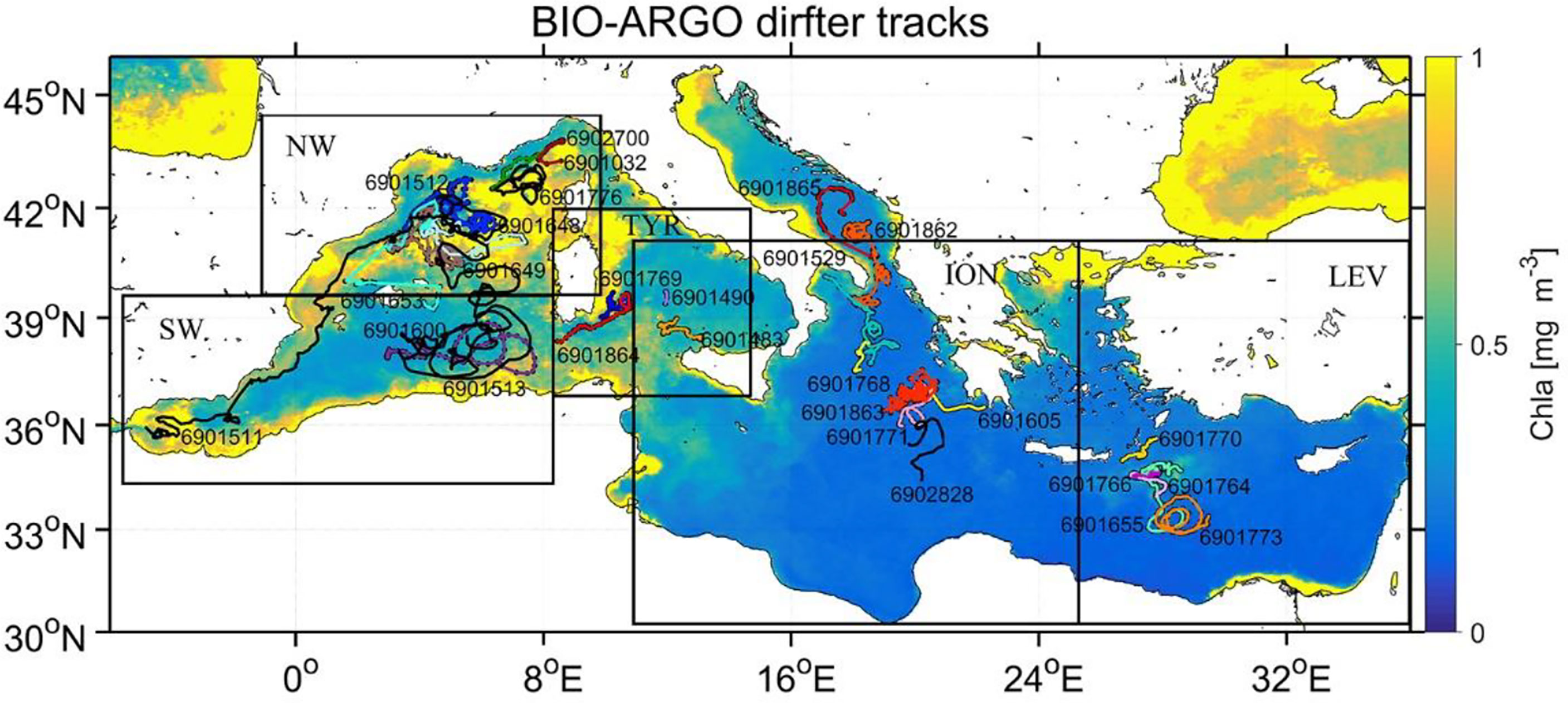
Figure 1 Spatial extent of the Mediterranean Sea and subregions divided in this study. The lines in different colors indicate the trajectories of the different Bio-Argo cruises. The background colors of the Mediterranean Sea indicate the monthly average Chl-a surface concentration derived from MODIS-Aqua data in March 2015.

2.2 BGC-Argo Chl-a Profiles

More than 70 BGC-Argo floats deployed between 2012 and 2016 alone (Cossarini et al., 2019). The long-term deployment has made the Mediterranean BGC-Argo network one of the densest networks in the global ocean in terms of the number of profiles per unit surface area, providing unique data support for studying ecosystem characteristics and dynamics.

In this study, Mediterranean Chl-a vertical profiles were obtained from a global database of vertical profiles derived from Biogeochemical Argo float measurements publicly available at https://www.seanoe.org/data/00383/49388/ (Marie et al., 2017). This dataset includes 0-1000 m vertical profiles of bio-optical and biogeochemical variables acquired by autonomous profiling BGC-Argo floats around local noon between October 2012 and January 2016. It contains profiles of downward irradiance at 3 wavelengths (380, 412 and 490 nm), photosynthetically available radiation, Chl-a concentration, fluorescent dissolved organic matter, and particle light backscattering at 700 nm. All variables have been quality controlled following specifically-developed procedures, and data corruption by biofouling and any instrumental drift has also been verified. In the Mediterranean Sea, all Chl-a profiles were collected by 27 BGC-Argo profiling floats, and their trajectories o are shown in Figure 1, with the various floats highlighted in different colors.

As a result, a total of 1611 Chl-a vertical profiles can be matched with other data used. To match up in situ Chl-a vertical profiles with other data, a 1°×1° box centered on each float location was adopted. These profiles were collected within a wide geographical area of the Mediterranean Sea in almost equal numbers during each season, with a total of 409, 411, 415 and 376 records measured in spring, summer, autumn and winter, respectively. Therefore, these profiles could represent the spatial and temporal characteristics of the phytoplankton vertical distribution in this basin.

2.3 GLBa0.08 Analysis Data

The 5-year product (from 2012 to 2016) of the Hybrid Coordinate Ocean Model–Navy Coupled Ocean Data Assimilation (HYCOM+NCODA) global 1/12° analysis (GLBa0.08; https://www.hycom.org/dataserver/gofs-3pt0/analysis) product was used in this study. The HYCOM Consortium is a nearly real-time global ocean prediction system based on the Hybrid Coordinate Ocean Model (HYCOM) and Navy Coupled Ocean Data Assimilation (NCODA) system (Halliwell, 2004). The advantage of HYCOM-based analysis is the implementation of a substantially evolved hybrid vertical coordinate system, which remains isopycnic in the well-stratified open ocean and combines different types of coordinates, transiting into level coordinates in less stratified regions (surface mixed layer) and very shallow water and into terrain-following sigma coordinates in nearshore regions (Chassignet et al., 2007). This feature provides the HYCOM with the ability to optimally simulate coastal and open ocean circulations.

GLBa0.08 is a uniformly gridded (1/12°) global reanalysis dataset that converts native HYCOM [ab] data into NetCDF data on a native Mercator–curvilinear HYCOM horizontal grid, interpolated into 33 z-levels (Shu et al., 2014). This product provides 11 ocean essential variables, such as the surface water flux, salinity, surface salinity trend, surface temperature trend, and mixed layer depth (MLD) (Augusto Souza Tanajura et al., 2014). All these data are freely available at https://www.hycom.org/dataserver/gofs-3pt0/analysis. In this research, only MLD products pertaining to the study period were utilized.

2.4 Satellite Data

Daily and monthly Moderate Resolution Imaging Spectroradiometer (MODIS) level-2 Chl-a product from 2011 to 2018 was used in this study. This product is generated with an empirical relationship derived from in situ measurements of Chl-a and remote sensing reflectance in the blue-to -green region of the visible spectrum (Hu et al., 2012). This product is produced by the NASA Ocean Color program and is available from https://oceancolor.gsfc.nasa.gov/cgi.

In addition to the Chl-a surface concentration, the euphotic layer depth (z_eu) has been verified as a main variable explaining the vertical variability in Chl-a along the water column (Vadakke-Chanat and Shanmugam, 2020). The euphotic layer depth is a common indicator of water turbidity, defined as the depth at which irradiance is attenuated to 1% of the initial value at the surface (Tett, 1989; Dera, 1992). Consequently, the corresponding level-3 product of the MODIS diffuse attenuation coefficient for the downwelling irradiance at 490 nm (hereafter referred to as Kd490), which can be used to estimate the depth of the euphotic layer, was also employed in this study. The MODIS Kd490 product is produced under the GlobColour project and is freely available at http://globcolour.info/. Kd490 was generated following the model proposed by Lee et al. (2005) . In this study, the method proposed by Lin et al. (2016) was used to estimate the euphotic layer depth. The specific steps are as follows: (1) The diffuse attenuation coefficient for the downwelling irradiance of the usable solar radiation (USR) (KdUSR) was estimated from Kd490. USR represents the spectrally integrated solar irradiance within the spectral window of 400–560 nm, as defined by Lee et al. (2014) . (2) The depth of the euphotic layer was derived according to the equation proposed by Lin et al. (2016).

All these satellite data have undergone quality and flag assessments and are generated with a spatial resolution of 4 km. To match the BGC-Argo, satellite, and analysis data, the satellite and analysis data in a 1°×1° box centered on each float location were used to provide matchups.

3 Methods

3.1 Methodological Overview

First, all the BGC-Argo Chl-a profiles were clustered with the PCM, after which, a decision tree profile classification model was established based on a priori knowledge provided by the clustering results. Then, these profiles were parameterized with a modified Gaussian function. Finally, for each type of Chl-a profile, empirical relationships between the corresponding shape-dependent parameters derived from previous profile fitting and Chl-a surface concentration were established. A flowchart of these steps is drawn in Figure 2.

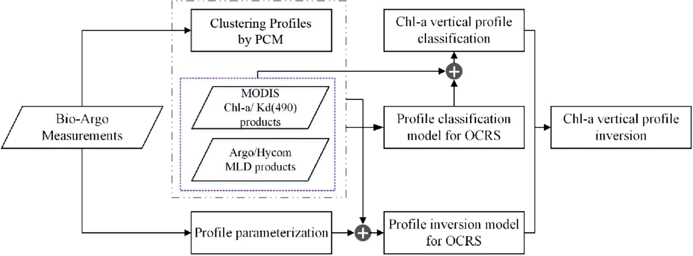
Figure 2 Flowchart of the proposed method for reconstructing Chl-a vertical profiles in the Mediterranean Sea.

3.2 Remote Sensing Pixel-Scale Chl-a Profile Type Identification

The vertical distribution of phytoplankton exhibits different shapes under the influence of the interactions between various biological (e.g., particular species present and physiological state) and physical (e.g., currents and shear between water parcels) factors, making it difficult to obtain one set of general parameters that can be applied to extrapolate all profiles. Therefore, a common practice is to classify vertical profiles according to their characteristics and to develop an extrapolation model for each of the subcategory. To more simply and objectively identify the profile type of each pixel of the remote sensing Chl-a product, the shape characteristics of Chl-a vertical profiles in the Mediterranean Sea were first explored by clustering all BGC-Argo Chl-a profiles. According to the profile clustering result, a binary tree profile classification model based on several publicly available marine essential variables was then established.

3.2.1 Revealing the Shape Characteristics of Chl-a Profiles

Next, the Chl-a vertical distribution in the Mediterranean Sea was explored with the PCM.

The PCM is an unsupervised machine learning classification technique designed to reveal the vertical distribution of ocean temperatures (Maze et al., 2017a). This method relies on a Gaussian mixture model (GMM) to decompose the probability density function (PDF) of a collection of profiles into a weighted sum of multidimensional Gaussian PDFs, thus facilitating the identification of the representative patterns of a given dataset (Maze et al., 2017a; Maze et al., 2017b). After classification, profiles within a given category are more similar to each other than they are to profiles in other categories (Jain et al., 1999).

The PCM was originally developed to characterize coherent heat patterns in the North Atlantic Ocean. Since it is more impartial than subjective grouping of profiles into classes, the PCM has since been successfully applied to characterize the vertical distributions of a variety of oceanographic variables (Boehme and Rosso, 2021). However, the performance of the PCM in the classification of Chl-a vertical profiles remains unclear and needs to be further explored.

Through objective and trial-and-error approaches, the Chl-a profiles in the Mediterranean Sea were ultimately categorized into four types with the PCM, and the shape characteristics of these profile types are shown in Figure 3. Referring to the previous literature (Lavigne et al., 2015), these four types were denoted as mixed, exponential, quasi-Gaussian and Gaussian types according to their shape characteristics. As shown in Figure 3, due to the presence of the MLD, the Chl-a concentration in all profile types remained almost constant at either a deep or a shallow depth. Specifically, the MLD was much deeper for the mixed type than for the other three profile types, resulting in almost constant mixed type profiles up to a certain depth. The Gaussian type profiles exhibited typical Gaussian distribution shapes, namely, curves with a concentration peak, and the Chl-a concentration decreased with increasing distance from the peak depth. Furthermore, the vertical profiles of the exponential and quasi-Gaussian types were roughly similar in shape, but these profiles differed greatly with regard to the range of specific concentrations, the presence of concentration peaks, and the depth at which the concentration declines.

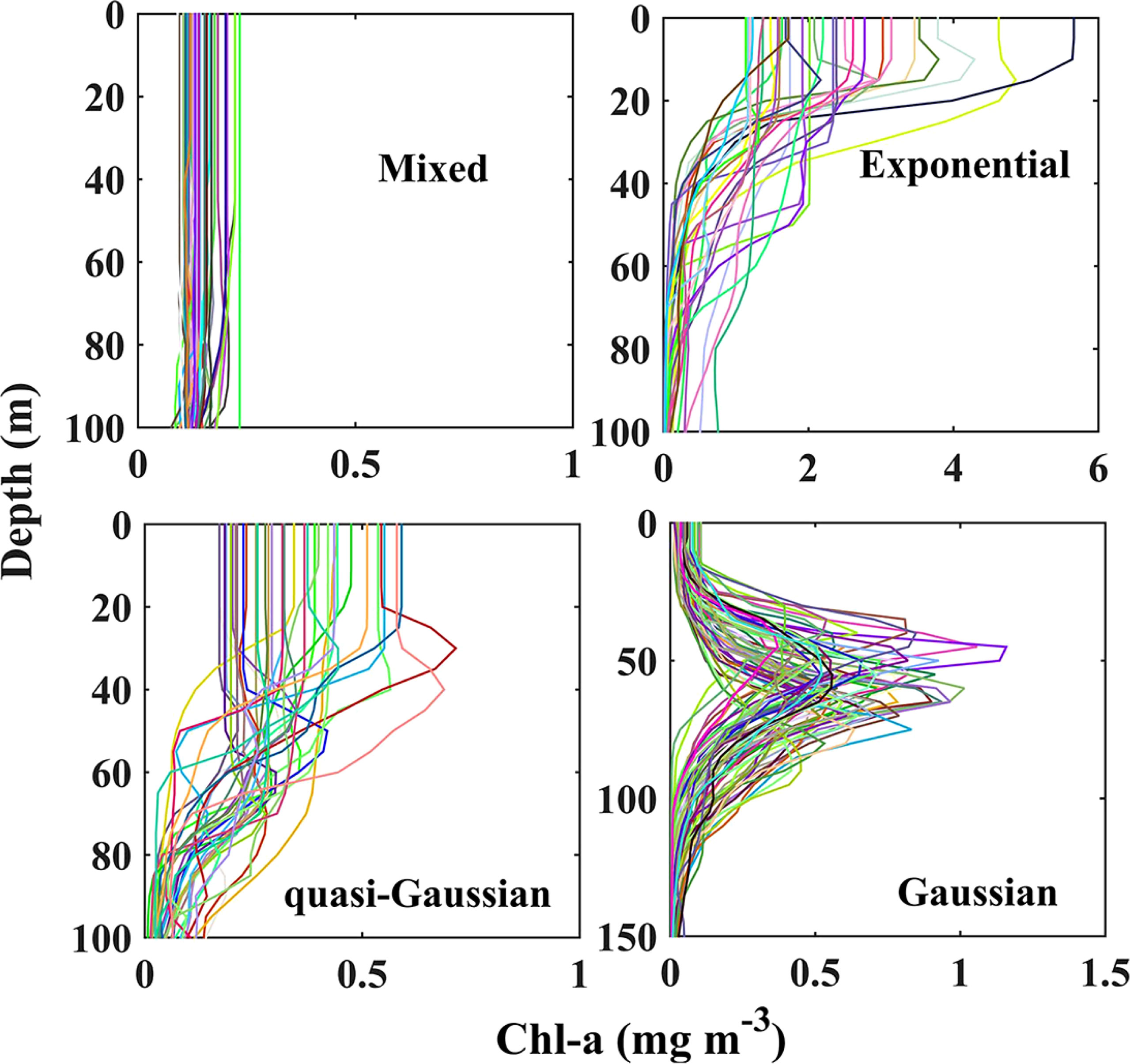
Figure 3 Typical shapes for each type of Chl-a vertical profile in the Mediterranean Sea.

3.2.2 Decision Tree Profile Classification Model

By analyzing the shape characteristics of these four types of Chl-a profiles and referring to the previous literature, the Chl-a surface concentration, euphotic layer depth and MLD were adopted in this study to establish a decision tree classification model to classify the type of each pixel of the remote sensing Chl-a product.

In general, Chl-a vertical distributions could be divided into two main types: uniform and nonuniform, corresponding to mixed and stratified water, respectively (Mignot et al., 2011). The differences between these two types of Chl-a vertical distributions in the Mediterranean Sea lies in whether the MLD exceeds the euphotic layer depth. For the uniform type profile, phytoplankton are nearly evenly distributed along the water column due to strong water mixing, resulting in a homogeneous Chl-a concentration from the surface to great depths. Hence, the ratio between the MLD and euphotic layer depth is a common indicator for the identification of deep mixed water (Uitz et al., 2006). Since the euphotic layer is the maximum depth of the light zone suitable for phytoplankton photosynthesis (Khanna et al., 2009) , when the euphotic layer is shallower than the mixed layer, the phytoplankton are almost uniformly distributed vertically.

As shown in Figure 3, the Gaussian, quasi-Gaussian and exponential types are all nonuniform due to the obvious presence of a subsurface chlorophyll maximum (SCM). By analyzing the shape characteristics of these three nonuniform profiles, the surface concentrations on the exponential type profiles were found to be much higher than those on the other two types of profiles (Figure 4). In addition, Gaussian profiles could be distinguished from quasi-Gaussian profiles based on the MLD.

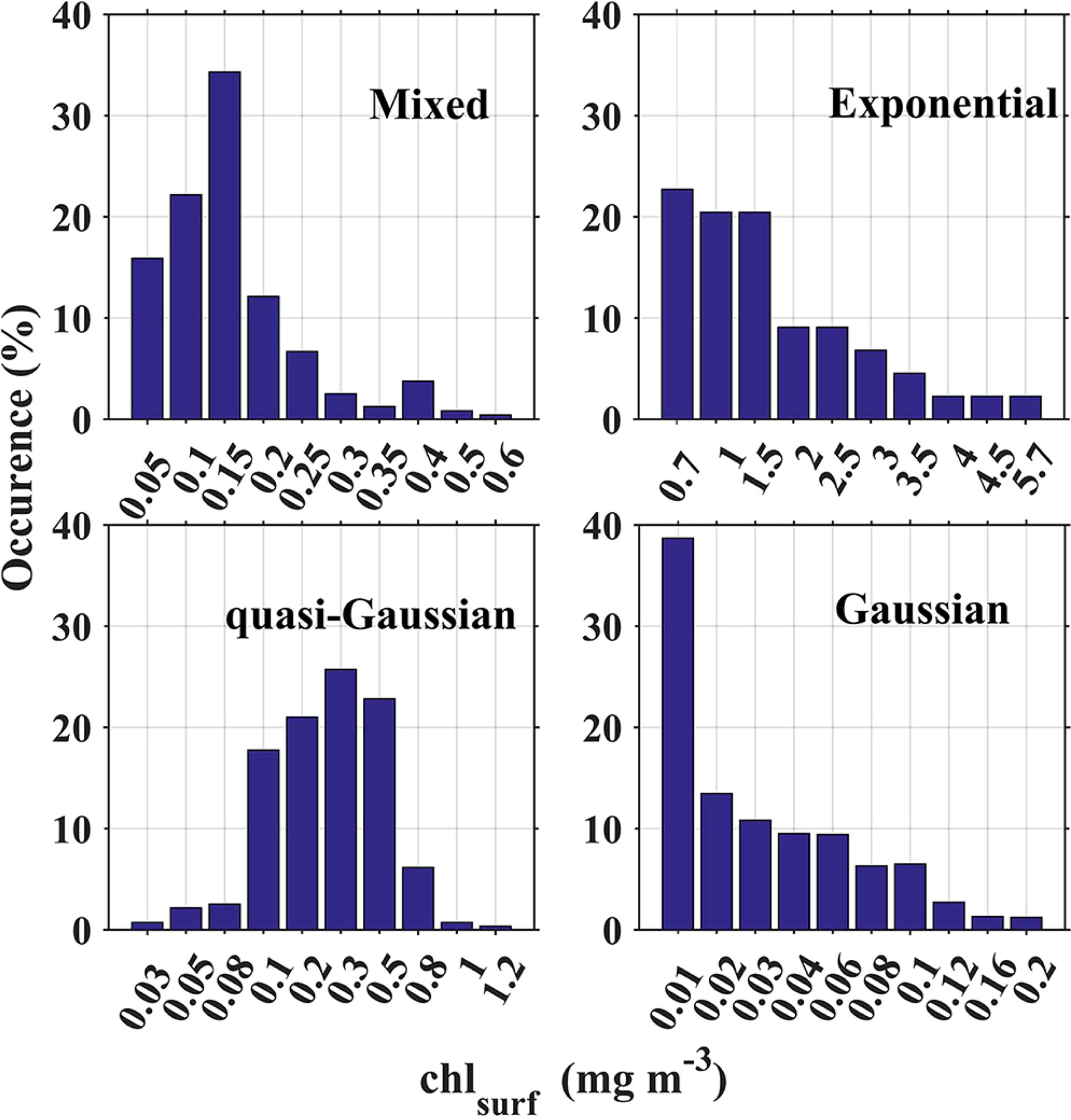
Figure 4 Surface concentrations of Chl-a on the different types of vertical profiles.

As a result, a binary tree based on the surface concentration, MLD and euphotic layer depth was developed to infer the vertical profile type in each pixel of the OCRS Chl-a product. As shown in Figure 5, the following three steps were included:

① A ratio of the MLD to the euphotic layer depth higher than 1 was adopted to identify profiles of the mixed type.

② A Chl-a surface concentration higher than 0.799 was used to recognize profiles of the exponential type.

③ Whether the MLD exceeded 31.1 m was considered to distinguish between Gaussian and quasi-Gaussian profiles. If the MLD exceeded this threshold, quasi-Gaussian profiles were determined; otherwise, Gaussian profiles were identified.

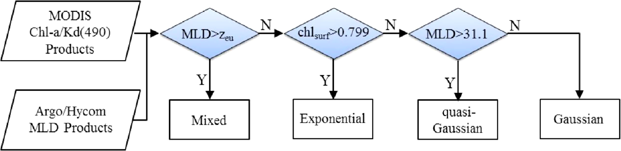
Figure 5 Flowchart of the Chl-a vertical profile classification model for the Mediterranean Sea.

3.3 In Situ Chl-a Profile Parameterization

To parameterize the profiles, each profile was fitted with a certain mathematical model, allowing the profile shape to be represented by model coefficients, which is a common practice in characterizing the profile shape of essential marine and atmospheric variables (Beckmann and Hense, 2007; González-Pola et al., 2007). Various functions have been used to parameterize marine variable vertical profiles, including Gaussian functions (Morel, 1988; Platt et al., 1988; Morel and Berthon, 1989) and their derivatives (Uitz et al., 2006), power functions (Liu et al., 2021) and exponential functions (Ardyna et al., 2013). Among these functions, the generalized (or shifted) Gaussian function is the most popular, and has been verified as a suitable function for fitting profiles containing only a single peak; this function is quite common in coastal, upwelling, open oceans and Arctic waters (Lewis et al., 1983; Siswanto et al., 2005). Here, to better characterize profiles with a shallow SCM layer, where the surface concentration is higher than the deepest value, the generalized Gaussian function was updated as a modified Gaussian function by replacing the constant with a linear function (Uitz et al., 2006). The general shapes of generalized and modified Gaussian functions are shown in Figure 6.

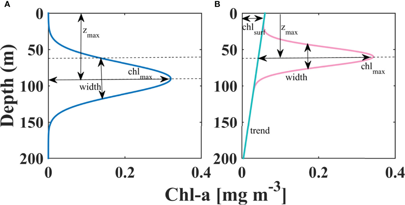
Figure 6 Shape difference between the generalized (A) and modified Gaussian (B) functions.

In this study, the modified Gaussian function was selected to parameterize the BGC-Argo Chl-a profiles. Since a mixed type Chl-a profile exhibits a constant concentration from the surface to great depths, these types of profiles were excluded from the subsequent parameterization to construct the inversion model. As a result, 1360 of the 1611 BGC-Argo Chl-a profiles were parameterized with the following:

where chl_surf denotes the Chl-a surface concentration measured by the BGC-Argo floats, trend indicates the trend of the background concentration, chl_max is the maximum concentration in the Chl-a profile, z_max denotes the maximum concentration depth, and width denotes the half-peak width, a fitting-related parameter indicating the thickness of the SCM that is defined as the width (measured in meters) at the half-height of the SCM layer. This fitting-related parameter is defined as controlling the shape of the profile but can be obtained only by model fitting and cannot be measured directly. According to the fitting formula used herein, the fitting-related parameters specifically refer to width and trend. Here, chl_max is regarded as the total magnitude of the Chl-a concentration, not that of the background-subtracted value.

To ensure the fitting accuracy, the Curve Fitting C program (O’Haver, 1997), a nonlinear iterative curve fitting method developed at the University of Maryland, was used to implement profile fitting. This method adjusts parameters in a systematic manner via a trial-and-error strategy until the equation yields a fitted curve that is close to the expected curve. Two commonly used fitting accuracy proxies, namely, the coefficient of determination (R²) and root-mean-square error (RMSE), were selected to evaluate the fitting effect. Overall, over 70% of the profiles had an R² greater than 0.8, and the mean R² was 0.93. In regard to the specific types, the Gaussian and exponential types attained the best fitting accuracy, both with an average R² of 0.94, followed by the quasi-Gaussian profile type with an average R² of 0.93. To illustrate the fitting effect more intuitively, panels (a), (b) and (c) of Figure 7 show example profiles with the highest fitting accuracy for each of these three types and their corresponding estimations. As shown in this figure, strong correlations were obtained between the measured and estimated vertical profiles, with R² values of 0.9873, 09942 and 0.9914 and RMSE values of 3.176, 2.80 and 3.825, respectively.

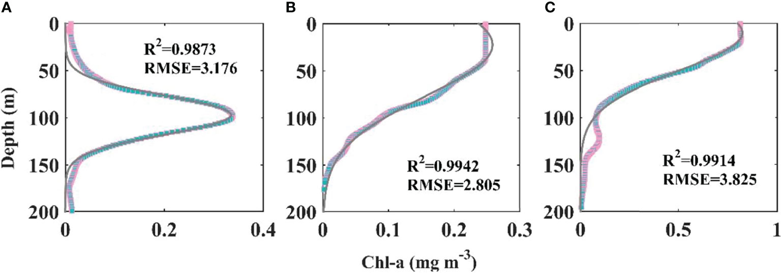
Figure 7 Fitting curves of the different types of Chl-a vertical profiles. Panels (A-C) show Gaussian, quasi-Gaussian and exponential profile types, respectively.

The statistical results (Table 1) for the shape-dependent parameters obtained after profile parameterization quantitatively confirmed the shape characteristics of each profile type mentioned in the previous section. Specifically, in terms of the average value, the Gaussian type yielded the lowest maximum Chl-a concentration but the greatest maximum Chl-a depth, with values of 0.4 mg m^-3 and 84.25 m, respectively. The exponential type was the opposite to the Gaussian type, namely, the highest maximum concentration and shallowest maximum concentration depth were obtained, at 2.03 mg m^-3 and 11.47 m, respectively. Compared to those of these two types of profiles, the maximum Chl-a concentration and corresponding depth of the quasi-Gaussian type were moderate, at 0.49 mg m^-3 and 38.21 m, respectively. In terms of the half-peak width, that of the quasi-Gaussian type was the largest (81.51 m), followed by the exponential (73.08 m) and Gaussian types (55.24 m). According to the half-peak width, phytoplankton were relatively more vertically concentrated along the Gaussian profile direction and more dispersed along the exponential and quasi-Gaussian profile directions, with half-peak widths of 55.24, 73.08 and 81.51 m, respectively. The trend variable is a model fitting-related parameter, with no explicit biophysical meaning, although this parameter can, to a certain extent, reflect the difference between the Chl-a surface concentration and the Chl-a concentration at great depths.

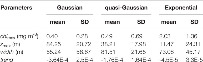
Table 1 Statistics for the shape-dependent parameters of the different types of Chl-a vertical profiles in the Mediterranean Sea.

3.4 Chl-a Vertical Profile Inversion Model

Reconstructing the Chl-a vertical profile from OCRS product is to establish the correlations between its surface variables and its shape-dependent parameters. Matchups between the BGC-Argo profiles and OCRS products provide the possibility to implement this inversion. After classifying and parameterizing the profile, the shape-dependent parameters of each profile were obtained. Then, the relationships between these shape-dependent parameters derived from the parameterization between their corresponding surface concentrations derived from the OCRS Chl-a products were analyzed. To ensure the robustness and accuracy of the established relationships, 487 poorly fitted profiles with R² values lower than 0.8 were discarded. As a result, 1124 robustly parameterized vertical profiles were retained to establish the vertical profile inversion model.

To establish the inversion model, all matchups were first used to reveal the global correlations applicable to all profile types. Only when robust global relationships cannot be obtained, the type-specific correlations were considered by using matchups corresponding to different type profiles. The SCM depth (z_max) has been demonstrated to be inversely proportional to the Chl-a concentration derived from satellite observations (chl_sat) over a wide range of trophic conditions (Morel & Berthon, 1989; Uitz et al., 2006; Mignot et al., 2011). This conclusion remains valid in the Mediterranean Sea. As shown in panel (a) of Figure 8, z_max had a strong negative correlation with chl_sat:

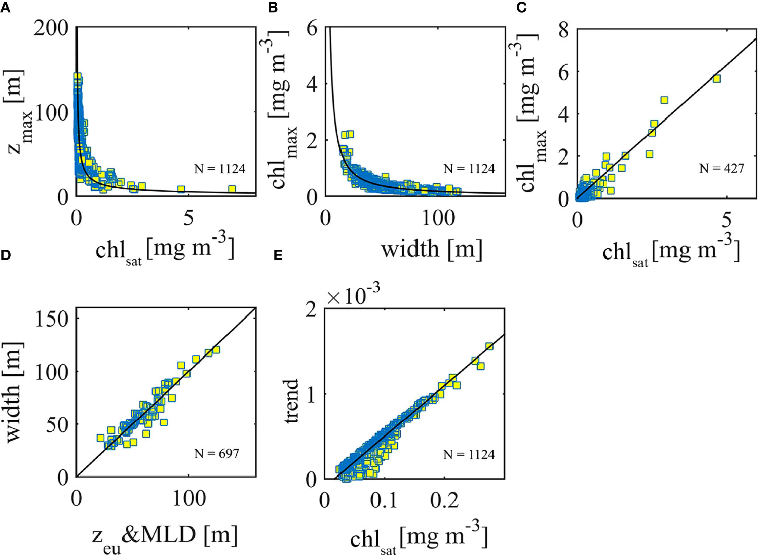
Figure 8 Relationships between the shape-dependent parameters of the Chl-a vertical profiles and the surface concentrations derived from the OCRS Chl-a products. (A, B, E) are global relationships observed from all BGC-Argo Chl-a profiles. (C, D) are type-dependent relationships obtained from quasi-Gaussian and Gaussian profiles, respectively.

This negative relationship was observed from all matchups with an R² value of 0.79, thus indicating this global correlation suitable to estimate z_max for all types of vertical profiles with chl_sat derived from OCRS products.

Panel (b) of Figure 8 shows the correlation between the maximum Chl-a concentration (chl_max) and half-peak width of the fitting curve (width) for all profile types. Similar to z_max and chl_sat, a strong negative correlation between chl_max and width was observed:

This formulation yielded an R² of 0.81. The relationship between the phytoplankton biomass maximum and SCM layer thickness is well understood, and thus, width was concluded to be closely correlated with chl_max in the study area. Notably, as the Chl-a maximum concentration rises, more phytoplankton accumulate within the SCM layer, nutrient consumption occurs more quickly, and the SCM layer becomes thinner (Barbieux et al., 2019).

In addition to these two relationships, another global correlation was observed between chl_sat and the background trend of the Chl-a concentration (trend):

The linear relationship between trend and chl_sat yielded an R² of 0.92, as shown in panel (e) of Figure 8. The potential reason for this negative relationship between these two parameters could be the positive correlation between the attenuation intensity of solar radiation and the phytoplankton biomass at the sea surface.

Having established the relationship between z_max and chl_sat and that between chl_max and width, the Chl-a vertical profile can be reconstructed only if the relationships between z_max or chl_sat with both chl_max and width can be established. However, except for the above parameters, no other reliable global correlations were discovered. Therefore, the possible correlations between these parameters and the combinations of the vertical profile types were explored via exploratory data analysis.

In regard to the quasi-Gaussian Chl-a vertical profiles, a strong positive linear correlation between chl_max and chl_sat was observed:

This linear relationship yielded an R² of 0.96. With this relationship, chl_max could be derived from the sea surface concentration measured by satellite sensors. Then, z_max can be derived from chl_sat via Eq. 2, and width can be estimated from the derived chl_max value based on Eq. 3. In this way, the quasi-Gaussian Chl-a vertical profile can be reconstructed.

In contrast to the quasi-Gaussian type, no direct relationships were found between chl_sat and chl_max or width in the Gaussian type profiles. Considering that the thickness of the subsurface layer is top–bottom limited by both light and nutrients, z_eu and the MLD were introduced here to estimate width. The variation in width with respect to z_eu and the MLD can be formulated as follows:

This correlation yielded an R² of 0.89. The establishment of this equation facilitates the estimation of all shape-dependent parameters of the Gaussian type Chl-a vertical profile. First, trend and z_max can be estimated based on the OCRS Chl-a products with Eqs. 2 and 4, respectively. Then, width can be calculated according to Eq. 6 based on the products of z_eu and MLD. Finally, chl_max can be derived from the estimated width according to Eq. 3.

Unfortunately, failure to determine the correlations between chl_sat and width and chl_max makes it impossible to reconstruct the exponential type Chl-a vertical profiles. Fortunately, few profiles were of this type (accounting for only 1.21% of all profiles) in the Mediterranean Sea, and thus, ignoring exponential type profiles would not significantly impact the inversion of Chl-a vertical profiles across the study region.

3.5 Accuracy Assessment Metrics

To evaluate the classification models, the most popular confusion matrix was selected in this study. Based on the selected confusion matrix, the overall accuracy (OA), user accuracy (UA) and producer accuracy (PA) were calculated. When deriving the confusion matrix, the labels provided by the PCM were regarded as the truth, and the labels obtained with the established vertical profile classification model were regarded as predictions.

To evaluate the profile inversion accuracy, the RMSE and the mean absolute percent deviation (MAPD) were selected as the accuracy metrics. Their mathematical equations are as follows:

where p_m denotes the shape-dependent parameter measured by the Bio-Argo profiling floats, p_e denotes the corresponding model estimation, and n indicates the number of vertical profiles used for evaluation.

4 Results

4.1 Spatial and Temporal Patterns of the in Situ Chl-a Vertical Profiles

To reveal the spatial and temporal patterns of the Chl-a vertical profiles in the Mediterranean Sea, the PCM classification results for all the profiles measured by the BGC-Argo floats were counted according to both the subsea area and the season, as shown in Figure 9. In general, as shown in the pie chart in panel (a) of this figure, the Gaussian type was the dominant Chl-a vertical profile type in the Mediterranean Sea, accounting for 78.48% of all measured profiles, followed by the mixed and quasi-Gaussian profile types, accounting for 15.6% and 4.72%, respectively. As mentioned above, the exponential type attained the lowest proportion, accounting for only 1.21% of all measured profiles. In terms of the spatial distribution, the Gaussian type was widely distributed in all five subsea areas, and the quasi-Gaussian type occurred in four subsea areas (all but LEV). The distribution of the mixed type was further reduced to the ION, LEV and NW subsea areas, whereas the exponential type was found only in the NW subsea area. In terms of the temporal distribution, the Gaussian type emerged mainly in summer, autumn and winter, while the exponential type occurred mostly in early summer. The mixed and quasi-Gaussian types were primarily observed in spring and summer but also in winter in some subsea areas.

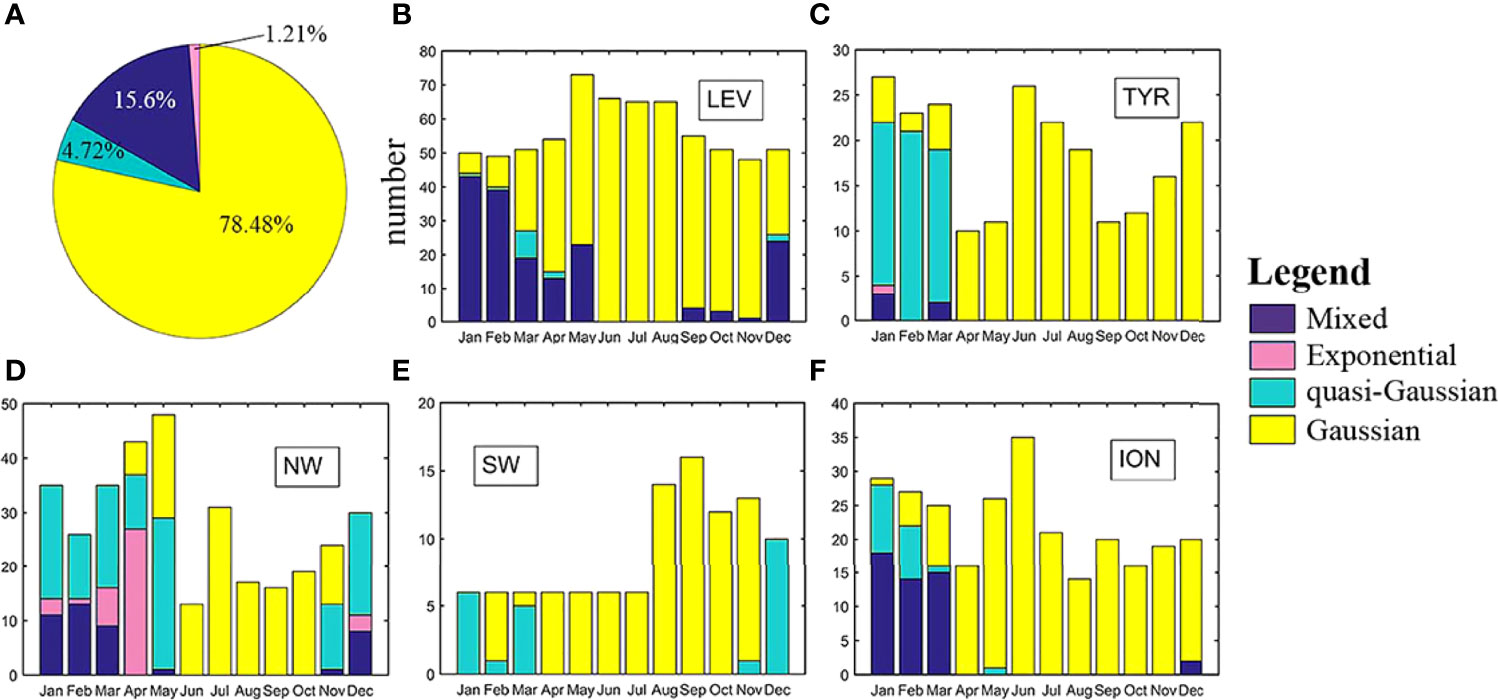
Figure 9 Spatial and temporal patterns of the Chl-a vertical profiles measured in the Mediterranean Sea. The pie chart in panel (A) shows the percentage of each profile type of all measurements. The histograms from panel (B–F) show the occurrence frequencies of the different types of Chl-a vertical profiles in the different subsea areas and seasons.

The spatial and temporal characteristics of the Chl-a vertical profiles revealed by the PCM agree with previous findings in Mediterranean bioregions (Mayot et al., 2017; Palmiéri et al., 2018). This agreement can be considered evidence that the classification results of the PCM can provide sufficiently accurate a priori knowledge for the construction of a vertical profile classification model.

4.2 Accuracy Assessment of the Proposed Profile Classification Model

The accuracy of the OCRS-based Chl-a vertical profile classification model was evaluated based on profiles measured by the four BGC-Argo floats reserved for validation with World Meteorological Organization (WMO) identifier numbers 6901511, 6901513, 6901776, and 6902828. As a result, 151 matchups were used to evaluate the performance of the trained binary tree profile classification model. Based on these matchups, the confusion matrix was calculated, as summarized in Table 2.

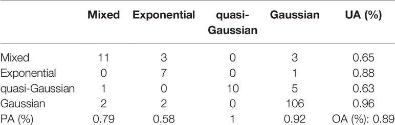
Table 2 Confusion matrix of Chl-a vertical profile classification (UA denotes the user accuracy and PA denotes the producer accuracy).

The confusion matrix reveals that the classification model achieved a satisfactory overall performance with an OA value of 89%. Specifically, the PA values of the Gaussian, quasi-Gaussian, exponential and mixed Chl-a vertical profile types were 92%, 100%, 58%, and 79%, respectively, and the corresponding UA values were 96%, 63%, 88%, and 65%. Regarding the dominant Gaussian Chl-a vertical profiles, the classification model achieved both very low omission errors and very low commission errors with PA and UA values of 92% and 96%, respectively. Although the PA values of the exponential type and UA values of the quasi-Gaussian and mixed types reached only 58%, 63% and 65%, respectively, this accuracy level is considered adequate considering their low proportion in the Mediterranean Sea. The OA value of the classification model reached 89%, which is sufficiently accurate to meet the needs of inverting Chl-a vertical profiles.

4.3 Accuracy Assessment of the Established Profile Inversion Model

The matchups used in the evaluation of the proposed classification model were also used to quantitatively assess the accuracy of the established vertical profile inversion model. The performance of the profile inversion model was assessed by measuring the deviations between the measured shape-dependent parameters and corresponding model estimations. Four parameters were used to characterize the Chl-a vertical profile shape in this study, but since width and trend cannot be directly measured, only chl_max and z_max were thus used for evaluation purposes to avoid possible uncertainties due to the profile parameterization.

Comparisons of chl_max and z_max estimated with the proposed profile inversion model with the corresponding reference in situ measurements are shown in panels (a) and (b), respectively, of Figure 10. Overall, a robust relationship was observed between the z_max values estimated with the inversion model based on the OCRS products and those measured by the BGC-Argo floats. This correlation was associated with a high determination coefficient (R^{2 =} 0.89) and low RMSE (8.49) and MAPD (6%) values. The slope of 0.89 indicates that the estimated values exhibited no significant deviation from the observed values. A satisfactory correlation was also observed between the estimated and measured chl_max values. Although the R² value and slope of the regression were lower at 0.64 and 0.72, respectively, and although the MAPD value increased to 22%, the correlation remained highly satisfactory given the large range of the study area.

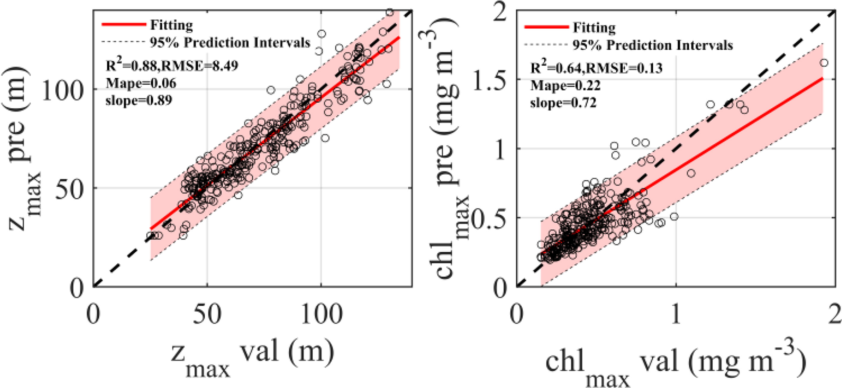
Figure 10 Shape-dependent parameters (z_max and chl_max) estimated with the proposed Chl-a vertical profile inversion model versus those measured by the BGC-Argo floats.

The accuracy of the proposed Chl-a profile inversion model was further evaluated for each of the different types of profiles (Table 3). In general, the inversion model achieved a higher accuracy for the Gaussian type than for the quasi-Gaussian type (R²: 0.62 versus 0.51; slope: 0.72 versus 0.33; RMSE: 0.13 versus 0.2; MAPD: 22% versus 37%).

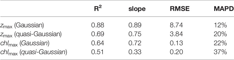
Table 3 Accuracy of the Chl-a vertical profile inversion model.

To compensate for the lack of evaluation results for width and trend, the Chl-a concentrations at the different depths estimated with the vertical profile inversion model were further compared to those measured by the BGC-Argo floats (Figure 11). Comparisons of the Chl-a concentrations at different depths can reveal not only the accuracy of the estimated width and trend values but also the overall accuracy of the profile inversion model. According to Figure 11, the predicted vertical profiles exhibited relatively high overall accuracy in all five subsea areas. The R² values were all higher than 0.5, and the RMSE values were all lower than 0.1. Among the specific subsea areas, the agreement between the actual measurements and predictions remained near the 1:1 line in the TYR, ION and LEV subsea areas. In contrast, in the SW and NW subsea areas, the regression lines were below the 1:1 line, indicating that the profile inversion model yielded slightly underestimated values, with R² values of 0.71 and 0.63, respectively.

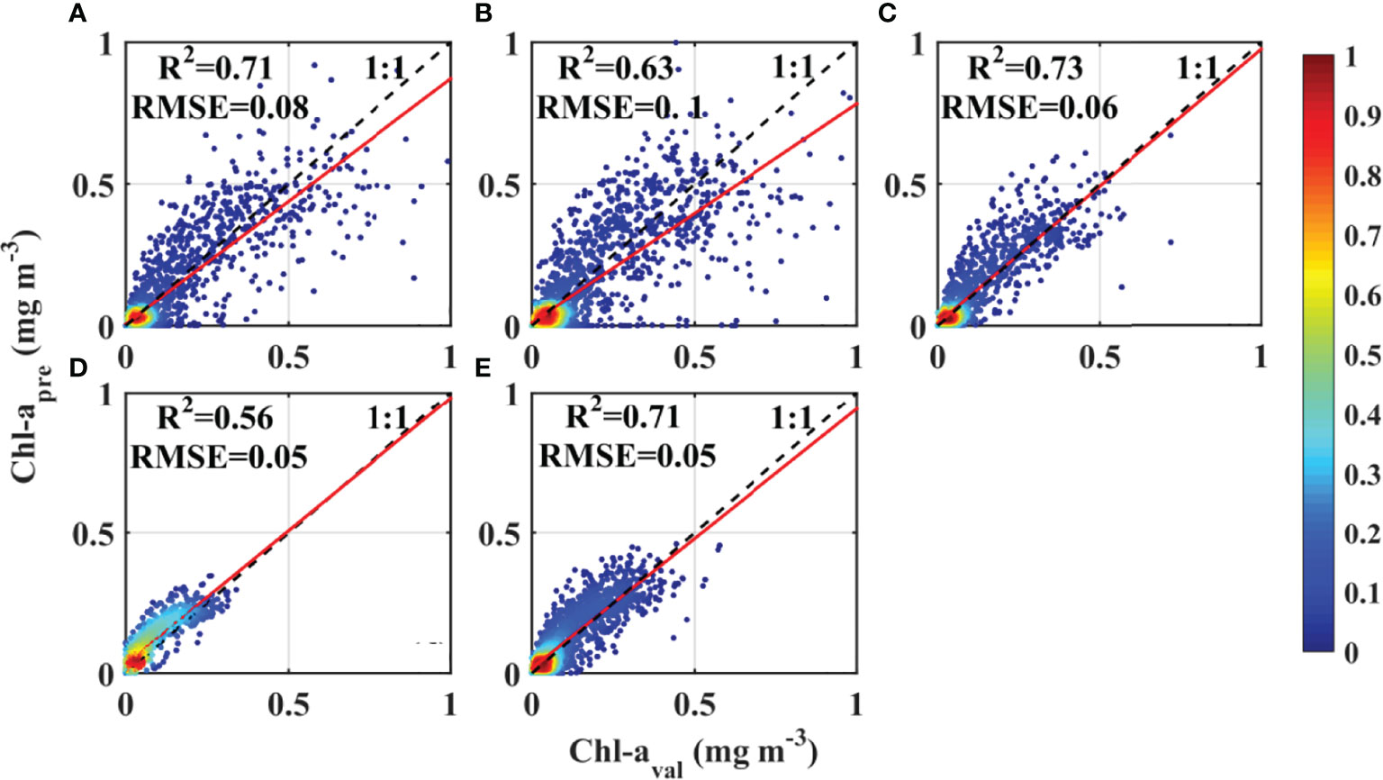
Figure 11 Scatterplots of the in situ Chl-a concentrations at different depths and those reconstructed via the method proposed in this study. Panels (A-E) successively show the comparisons for the SW, NW, TYR, ION and LEV subsea areas.

5 Discussion

5.1 Spatial and Temporal Characteristics of the Chl-a Profile Types in the Mediterranean Sea

To investigate the spatial characteristics of the Chl-a vertical profile types in the Mediterranean Sea, the monthly Chl-a profile types from 2011 to 2018 were generated based on the proposed Chl-a profile classification model, and the proportion of each type was determined. The results are shown in Figure 12, with the proportions of the mixed, exponential, quasi-Gaussian and Gaussian types being shown successively in panels (a) through (d). In general, the findings are consistent with the classification results of the PCM applied to the BGC-Argo Chl-a profiles, as introduced in Section 4.1. Specifically, the Gaussian type is the most common Chl-a profile type in the Mediterranean Sea, followed by the quasi-Gaussian, mixed, and exponential types. Moreover, the Gaussian type Chl-a profile is evenly distributed across the whole Mediterranean Sea, with a proportion higher than 50% in most of the areas, even exceeding 80% in the northern coastal area and near the Kerkennah Islands, a group of islands off the eastern coast of Tunisia. The quasi-Gaussian type attains a higher proportion in the southern half of the sea than in the northern half, with a maximum frequency of nearly 40%. The mixed type Chl-a profile is similar to the quasi-Gaussian type profile in terms of its maximum proportion, but its spatial distribution is the opposite, namely, the former profile type is concentrated mainly in the northern half of the sea.

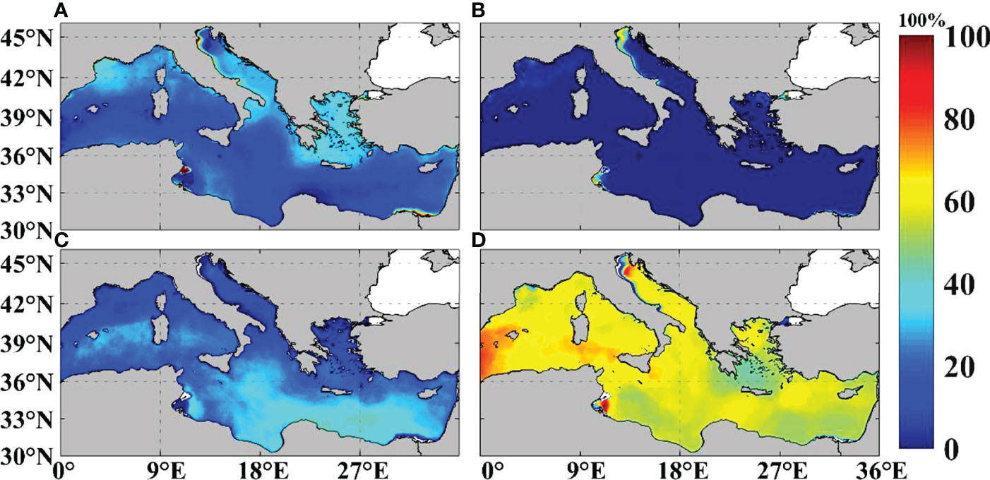
Figure 12 Proportion of each profile type in the Mediterranean Sea from 2011 to 2018. Panels (A-D) successively show the mixed, exponential, quasi-Gaussian and Gaussian types.

The temporal characteristics of the Chl-a vertical profile types in the Mediterranean Sea were analyzed by adopting the monthly Chl-a profile classification results in 2013 (depicted in Figure 13) as an example. This figure shows that the Mediterranean Chl-a vertical profile types exhibit obvious seasonal characteristics. Specifically, Gaussian type Chl-a vertical profiles are distributed mainly from March to November, and are dominant from April to October, in contrast, quasi-Gaussian type Chl-a vertical profiles are distributed largely from October to March of the following year, and appear to predominate in November, December and March. The time window of the quasi-Gaussian type profiles is similar to that of the mixed type profiles, but differently appears to predominate in January and February.

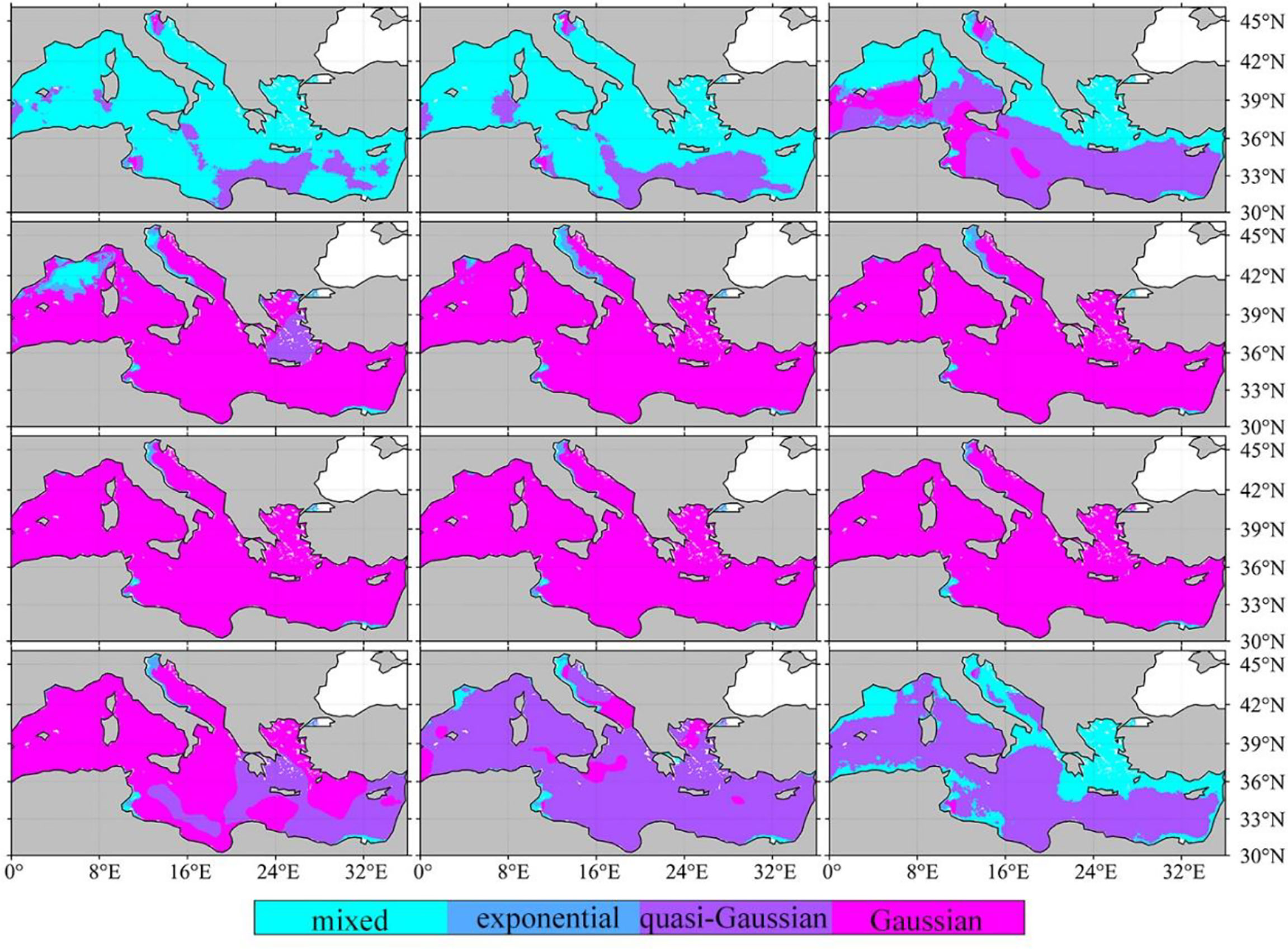
Figure 13 Monthly Chl-a profile types in the Mediterranean Sea in 2013. The subgraphs show January to December from top to bottom and left to right.

5.2 Spatial and Temporal Characteristics of the Chl-a Profile Shape-Dependent Parameters in the Mediterranean Sea

Based on the established Chl-a vertical profile classification and inversion models, the true Chl-a vertical profiles in the Mediterranean Sea can be visualized in 3D as long as the corresponding MODIS Chl-a and Kd490 products and HYCOM MLD product can be obtained. Continuous summer and autumn Chl-a concentrations in the Mediterranean were generated, for example, by using the June and September monthly MODIS Chl-a products and the monthly average MLD products. The Chl-a total concentration was further integrated according to the reconstructed vertical profiles.

To further verify the robustness of the proposed method, the characteristics of phytoplankton vertical distribution in the Mediterranean Sea revealed by the reconstruction results were compared to those reported in the literature. The per-pixel shape-dependent parameters and derived total Chl-a are shown in Figure 14, showing that the different shape-dependent parameters exhibit distinct spatial and temporal patterns. For example, in terms of their seasonality, z_max is deeper in summer than in autumn (mean depth of 88.54 ± 28.11 m versus 85.17 ± 24.94 m), while the width is larger in summer than in autumn (mean value of 64.36 ± 20.96 m versus 57.59 ± 18.67 m). However, chl_max reveals the opposite pattern, with a higher mean value in September (0.38 ± 0.18 mg m^-3) than in June (0.37 ± 0.15 mg m^-3), which agrees with previous findings (Lavigne et al., 2015). Spatially, z_max exhibits a longitudinal gradient in the Mediterranean Sea, with the value rising with increasing longitude up to a depth in excess of 120 m in the eastern Mediterranean Sea, except for some coastal areas. This conclusion agrees with previous findings reported by Lavigne et al. (2015) and Crise et al. (1999). A similar longitudinal gradient is also observed for width, which is larger in the eastern than in the western Mediterranean Sea. Furthermore, the existence of an east–west gradients of these shape-dependent parameters directly leads to a similar gradient of the Chl-a total concentration. As a result, the Chl-a total concentration is higher in the eastern Mediterranean Sea than in the western Mediterranean Sea in both summer and autumn.

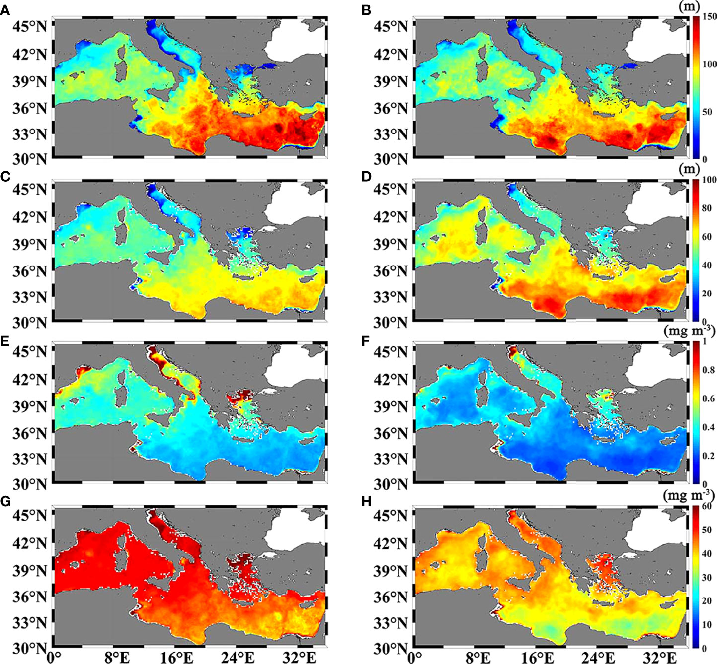
Figure 14 Monthly Chl-a vertical profile reconstruction results for June and September via OCRS. Panels (A), (C), (E) and (G) show z_max, width, chl_max and the Chl-a total concentration in June, respectively. Panels (B), (D), (F) and (H) show these parameters in September.

6 Conclusions and Perspectives

To observe the 3D spatial and temporal Chl-a concentration distribution in the Mediterranean Sea, a simple and robust process-oriented profile reconstruction method was proposed in this study. To estimate Chl-a vertical profiles based on corresponding OCRS products, the established vertical profile classification model was first used to identify the profile type in each of the pixels of the Chl-a product based on both Kd490 and MLD products, and the shape-dependent parameters of the vertical profiles were then estimated by using type-related correlations based on the proposed profile inversion model. A quantitative evaluation revealed that the proposed vertical profile classification model achieved an overall accuracy of 89%, and the proposed vertical profile inversion model attained an average absolute percent deviation value ranging from 12% to 37% for the different shape-dependent parameters.

The proposed profile estimation method was then used to generate monthly 3D Chl-a profiles in the Mediterranean Sea from 2011 to 2018. Based on the reconstructed Chl-a profiles, their spatial and temporal characteristics and those of the water column total biomass in the Mediterranean Sea were investigated. Considering the important role of that Mediterranean Sea plays in climate change research, the proposed method is expected to serve as a powerful tool in studying the status and changes in the Earth’s environment.

Data Availability Statement

The raw data supporting the conclusions of this article will be made available by the authors, without undue reservation.

Author Contributions

XL: Investigation, Conceptualization, Data curation, Methodology, Writing-Original draft. ZM: Supervision, Methodology, Reviewing. HZ: Validation, Editing, Methodology, Reviewing. WZ: Reviewing and Editing. DY: Methodology and Editing. YoL: Reviewing and Editing. ZW: Editing. YuL: Editing. All authors contributed to the article and approved the submitted version.

Funding

This study is supported by the High Resolution Earth Observation Systems of National Science and Technology Major Projects (05-Y30B01-9001-19/20-2); Key Special Project for Introduced Talents Team of Southern Marine Science and Engineering Guangdong Laboratory (Guangzhou) (GML2019ZD0602); the National Science Foundation of China (61991454); the National Key Research and Development Program of China (2016YFC1400901).

Conflict of Interest

The authors declare that the research was conducted in the absence of any commercial or financial relationships that could be construed as a potential conflict of interest.

Publisher’s Note

All claims expressed in this article are solely those of the authors and do not necessarily represent those of their affiliated organizations, or those of the publisher, the editors and the reviewers. Any product that may be evaluated in this article, or claim that may be made by its manufacturer, is not guaranteed or endorsed by the publisher.

References

Ardyna M., Babin M., Gosselin M., Devred E., Bélanger S., Matsuoka A., et al. (2013). Parameterization of Vertical Chlorophyll a in the Arctic Ocean: Impact of the Subsurface Chlorophyll Maximum on Regional, Seasonal, and Annual Primary Production Estimates. Biogeosciences 10 (6), 4383–4404. doi: 10.5194/bg-10-4383-2013
Augusto Souza Tanajura C., Novaes Santana A., Mignac D., Nascimento Lima L., Belyaev K., Ji-Ping X. (2014). The REMO Ocean Data Assimilation System Into HYCOM (RODAS_H): General Description and Preliminary Results. Atmosph. Ocean. Sci. Lett. 7 (5), 464–470. doi: 10.3878/j.issn.1674-2834.14.0011
Barbieux M., Uitz J., Gentili B., Pasqueron de Fommervault O., Mignot A., Poteau A., et al. (2019). Bio-Optical Characterization of Subsurface Chlorophyll Maxima in the Mediterranean Sea From a Biogeochemical-Argo Float Database. Biogeosciences 16 (6), 1321–1342. doi: 10.5194/bg-16-1321-2019
Beckmann A., Hense I. (2007). Beneath the Surface: Characteristics of Oceanic Ecosystems Under Weak Mixing Conditions – A Theoretical Investigation. Prog. Oceanogr. 75 (4), 771–796. doi: 10.1016/j.pocean.2007.09.002
Boehme L., Rosso I. (2021). Classifying Oceanographic Structures in the Amundsen Sea, Antarctica. Geophys. Res. Lett. 48 (5), e2020GL089412. doi: 10.1029/2020GL089412
Charantonis A. A., Badran F., Thiria S. (2015). Retrieving the Evolution of Vertical Profiles of Chlorophyll-A From Satellite Observations Using Hidden Markov Models and Self-Organizing Topological Maps. Remote Sens. Environ. 163, 229–239. doi: 10.1016/j.rse.2015.03.019
Chassignet E. P., Hurlburt H. E., Smedstad O. M., Halliwell G. R., Hogan P. J., Wallcraft A. J., et al. (2007). The HYCOM (HYbrid Coordinate Ocean Model) Data Assimilative System. J. Mar. Syst. 65 (1), 60–83. doi: 10.1016/j.jmarsys.2005.09.016
Cossarini G., Mariotti L., Feudale L., Mignot A., Salon S., Taillandier V., et al. (2019). Towards Operational 3d-Var Assimilation of Chlorophyll Biogeochemical-Argo Float Data Into a Biogeochemical Model of the Mediterranean Sea. Ocean. Model. 133, 112–128. doi: 10.1016/j.ocemod.2018.11.005
Crise A., Allen J. I., Baretta J., Crispi G., Mosetti R., Solidoro C. (1999). The Mediterranean Pelagic Ecosystem Response to Physical Forcing. Prog. Oceanogr. 44 (1), 219–243. doi: 10.1016/S0079-6611(99)00027-0
Dierssen H. M. (2010). Perspectives on Empirical Approaches for Ocean Color Remote Sensing of Chlorophyll in a Changing Climate. Proc. Natl. Acad. Sci. 107 (40), 17073–17078. doi: 10.1073/pnas.0913800107
Erickson Z. K., Frankenberg C., Thompson D. R., Thompson A. F., Gierach M. (2019). Remote Sensing of Chlorophyll Fluorescence in the Ocean Using Imaging Spectrometry: Toward a Vertical Profile of Fluorescence. Geophys. Res. Lett. 46 (3), 1571–1579. doi: 10.1029/2018GL081273
Falkowski P. (2012). Ocean Science: The Power of Plankton. Nature 483 (7387), S17–S20. doi: 10.1038/483S17a
González-Pola C., Fernández-Díaz J. M., Lavín A. (2007). Vertical Structure of the Upper Ocean From Profiles Fitted to Physically Consistent Functional Forms. Deep. Sea. Res. Part I.: Oceanogr. Res. Pap. 54 (11), 1985–2004. doi: 10.1016/j.dsr.2007.08.007
Gordon H. R., Clark D. K., Mueller J. L., Hovis W. A. (1980). Phytoplankton Pigments From the Nimbus-7 Coastal Zone Color Scanner: Comparisons With Surface Measurements. Science 210 (4465), 63–66. doi: 10.1126/science.210.4465.63
Halliwell G. R. (2004). Evaluation of Vertical Coordinate and Vertical Mixing Algorithms in the HYbrid-Coordinate Ocean Model (HYCOM). Ocean. Model. 7 (3), 285–322. doi: 10.1016/j.ocemod.2003.10.002
Hu C., Lee Z., Franz B. (2012). Chlorophyll a Algorithms for Oligotrophic Oceans: A Novel Approach Based on Three-Band Reflectance Difference. J. Geophys. Res.: Ocean. 117 (C1). doi: 10.1029/2011JC007395
Jain A. K, Murty M. N, Flynn P. J. (1999). Data clustering: a review. ACM computing surveys (CSUR). 31(3), 264–323. doi: 10.1145/331499.331504
Khanna D., Bhutiani R., Chandra K. S. (2009). Effect of the Euphotic Depth and Mixing Depth on Phytoplanktonic Growth Mechanism. Int. J. Environ. Res. 3 (2), 223–28. doi: 10.22059/IJER.2010.49
Kotta D., Kitsiou D. (2019). Chlorophyll in the Eastern Mediterranean Sea: Correlations With Environmental Factors and Trends. Environments 6 (8), 98. doi: 10.3390/environments6080098
Lavigne H., D'Ortenzio F., Ribera D'Alcalà M., Claustre H., Sauzède R., Gacic M. (2015). On the Vertical Distribution of the Chlorophyll a Concentration in the Mediterranean Sea: A Basin-Scale and Seasonal Approach. Biogeosciences 12 (16), 5021–5039. doi: 10.5194/bg-12-5021-2015
Lee Z., Du K., Arnone R. (2005). A Model for the Diffuse Attenuation Coefficient of Downwelling Irradiance. J. Geophys. Res.: Ocean. 110 (C2). doi: 10.1029/2004JC002275
Lee Y. J., Matrai P. A., Friedrichs M. A., Saba V. S., Antoine D., Ardyna M., et al. (2015). An Assessment of Phytoplankton Primary Productivity in the Arctic Ocean From Satellite Ocean Color/in Situ Chlorophyll-A Based Models. J. Geophys. Res.: Ocean. 120 (9), 6508–6541. doi: 10.1002/2015JC011018
Lee Z., Shang S., Du K., Wei J., Arnone R. (2014). Usable Solar Radiation and its Attenuation in the Upper Water Column. J. Geophys. Res.: Ocean. 119 (2), 1488–1497. doi: 10.1002/2013JC009507
Lewis M. R., Cullen J. J., Platt T. (1983). Phytoplankton and Thermal Structure in the Upper Ocean: Consequences of Nonuniformity in Chlorophyll Profile. J. Geophys. Res.: Ocean. 88 (C4), 2565–2570. doi: 10.1029/JC088iC04p02565
Lin J., Lee Z., Ondrusek M., Kahru M. (2016). Attenuation Coefficient of Usable Solar Radiation of the Global Oceans. J. Geophys. Res.: Ocean. 121 (5), 3228–3236. doi: 10.1002/2015JC011528
Liu D., Yu S., Cao Z., Qi T., Duan H. (2021). Process-Oriented Estimation of Column-Integrated Algal Biomass in Eutrophic Lakes by MODIS/Aqua. Int. J. Appl. Earth Observ. Geoinfo. 99, 102321. doi: 10.1016/j.jag.2021.102321
Barbieux M., Organell E., Claustre H., et al. (2017). A Global Database of Vertical Profiles Derived From Biogeochemical Argo Float Measurements for Biogeochemical and Bio-Optical Applications. SEANOE. doi: 10.17882/49388
Mayot N., D'Ortenzio F., Taillandier V., Prieur L., de Fommervault O. P., Claustre H., et al. (2017). Physical and Biogeochemical Controls of the Phytoplankton Blooms in North Western Mediterranean Sea: A Multiplatform Approach Over a Complete Annual Cycle, (2012–2013 DEWEX Experiment). J. Geophys. Res.: Ocean. 122 (12), 9999–10019. doi: 10.1002/2016JC012052
Maze G., Mercier H., Cabanes C. (2017a). Profile Classification Models. Mercator. Ocean. J. 55), 48–56.
Maze G., Mercier H., Fablet R., Tandeo P., Radcenco M. L., Lenca P., et al. (2017b). Coherent Heat Patterns Revealed by Unsupervised Classification of Argo Temperature Profiles in the North Atlantic Ocean. Prog. Oceanogr. 151, 275–292. J. P. i. O. doi: 10.1016/j.pocean.2016.12.008
McClain C. R. (2009). A Decade of Satellite Ocean Color Observations. Annu. Rev. Mar. Sci. 1 (1), 19–42. doi: 10.1146/annurev.marine.010908.163650
Mignot A., Claustre H., D'Ortenzio F., Xing X., Poteau A., Ras J. (2011). From the Shape of the Vertical Profile of In Vivo Fluorescence to Chlorophyll-A Concentration. Biogeosciences 8 (8), 2391–2406. doi: 10.5194/bg-8-2391-2011
Millán-Núñez R., Alvarez-Borrego S., Trees C. C. (1997). Modeling the Vertical Distribution of Chlorophyll in the California Current System. J. Geophys. Res.: Ocean. 102 (C4), 8587–8595. doi: 10.1029/97JC00079
Morel A. (1988). Optical Modeling of the Upper Ocean in Relation to its Biogenous Matter Content (Case I Waters). J. Geophys. Res.: Ocean. 93 (C9), 10749–10768. doi: 10.1029/JC093iC09p10749
Morel A., Berthon J.-F. (1989). Surface Pigments, Algal Biomass Profiles, and Potential Production of the Euphotic Layer: Relationships Reinvestigated in View of Remote-Sensing Applications. Limnol. Oceanogr. 34 (8), 1545–1562. doi: 10.4319/lo.1989.34.8.1545
O’Haver T. (1997). A Pragmatic Introduction to Signal Processing (University of Maryland at College Park). https://terpconnect.umd.edu/~toh/spectrum/CurveFittingC.html.
Palmiéri J., Dutay J. C., D'Ortenzio F., Houpert L., Mayot N., Bopp L. (2018). The Mediterranean Subsurface Phytoplankton Dynamics and Their Impact on Mediterranean Bioregions. Biogeosci. Discuss. 2018, 1–38. doi: 10.5194/bg-2018-423
Pisano A., Marullo S., Artale V., Falcini F., Yang C., Leonelli F. E., et al. (2020). New Evidence of Mediterranean Climate Change and Variability From Sea Surface Temperature Observations. Remote Sens. 12 (1), 132. doi: 10.3390/rs12010132
Platt T., Sathyendranath S. (1988). Oceanic Primary Production: Estimation by Remote Sensing at Local and Regional Scales. Science 241 (4873), 1613–1620. doi: 10.1126/science.241.4873.1613
Platt T., Sathyendranath S., Caverhill C. M., Lewis M. R. (1988). Ocean Primary Production and Available Light: Further Algorithms for Remote Sensing. Deep. Sea. Res. Part A. Oceanogr. Res. Pap. 35 (6), 855–879. doi: 10.1016/0198-0149(88)90064-7
Puissant A., El Hourany R., Charantonis A. A., Bowler C., Thiria S. (2021). Inversion of Phytoplankton Pigment Vertical Profiles From Satellite Data Using Machine Learning. Remote Sens. 13 (8), 1445. doi: 10.3390/rs13081445
Robinson A. R., Leslie W. G., Theocharis A., Lascaratos A. (2001). Mediterranean Sea Circulation. Steele J. H. (Ed.), Encyclopedia of Ocean Sciences, pp.1689–1705. (Oxford:Academic Press)
Sammartino M., Buongiorno Nardelli B., Marullo S., Santoleri R. (2020). An Artificial Neural Network to Infer the Mediterranean 3d Chlorophyll-A and Temperature Fields From Remote Sensing Observations. Remote Sens. 12 (24), 4123. doi: 10.3390/rs12244123
Sammartino M., Marullo S., Santoleri R., Scardi M. (2018). Modelling the Vertical Distribution of Phytoplankton Biomass in the Mediterranean Sea From Satellite Data: A Neural Network Approach. Remote Sens. 10 (10), 1666. doi: 10.3390/rs10101666
Sauzède R., Claustre H., Jamet C., Uitz J., Ras J., Mignot A., et al. (2015). Retrieving the Vertical Distribution of Chlorophyll a Concentration and Phytoplankton Community Composition From in Situ Fluorescence Profiles: A Method Based on a Neural Network With Potential for Global-Scale Applications. J. Geophys. Res.: Ocean. 120 (1), 451–470. doi: 10.1002/2014JC010355
Shu Y., Xue H., Wang D., Chai F., Xie Q., Yao J., et al. (2014). Meridional Overturning Circulation in the South China Sea Envisioned From the High-Resolution Global Reanalysis Data Glba0.08. J. Geophys. Res.: Ocean. 119 (5), 3012–3028. doi: 10.1002/2013JC009583
Silulwane N., Richardson A., Shillington F., Mitchell-Innes B. (2001). Identification and Classification of Vertical Chlorophyll Patterns in the Benguela Upwelling System and Angola-Benguela Front Using an Artificial Neural Network. Afr. J. Mar. Sci. 23, 37–51. doi: 10.2989/025776101784528872
Siswanto E., Ishizaka J., Yokouchi K. (2005). Estimating Chlorophyll-A Vertical Profiles From Satellite Data and the Implication for Primary Production in the Kuroshio Front of the East China Sea. J. Oceanogr. 61 (3), 575–589. doi: 10.1007/s10872-005-0066-7
Tett P. (1989). The Photic Zone. In Light and Life in the Sea (Pp. 59-87) (Plymouth, United Kingdom:Cambridge University Press).
Uitz J., Claustre H., Morel A., Hooker S. B. (2006). Vertical Distribution of Phytoplankton Communities in Open Ocean: An Assessment Based on Surface Chlorophyll. J. Geophys. Res.: Ocean. 111 (C8). doi: 10.1029/2005JC003207
Vadakke-Chanat S., Shanmugam P. (2020). A Model for the Vertical Chlorophyll-A Distribution in the Bay of Bengal Using Remote Sensing Data. IEEE Trans. Geosci. Remote Sens. 58 (1), 704–712. doi: 10.1109/TGRS.2019.2939548
Keywords: Chl-a, profile reconstruction, modis, BGC-Argo, mediterranean
Citation: Li X, Mao Z, Zheng H, Zhang W, Yuan D, Li Y, Wang Z and Liu Y (2022) Process-Oriented Estimation of Chlorophyll-a Vertical Profile in the Mediterranean Sea Using MODIS and Oceanographic Float Products. Front. Mar. Sci. 9:933680. doi: 10.3389/fmars.2022.933680
Received: 01 May 2022; Accepted: 23 May 2022;
Published: 24 June 2022.
Edited by:
Weiwei Sun, Ningbo University, ChinaReviewed by:
Changchun Huang, Nanjing Normal University, ChinaDeyong Sun, Nanjing University of Information Science and Technology, China
Kun Shi, Chinese Academy of Sciences (CAS), China
Copyright © 2022 Li, Mao, Zheng, Zhang, Yuan, Li, Wang and Liu. This is an open-access article distributed under the terms of the Creative Commons Attribution License (CC BY). The use, distribution or reproduction in other forums is permitted, provided the original author(s) and the copyright owner(s) are credited and that the original publication in this journal is cited, in accordance with accepted academic practice. No use, distribution or reproduction is permitted which does not comply with these terms.
*Correspondence: Zhihua Mao, mao@sio.org.cn