


Introduction
Phase-contrast images possess high contrast between cells and the background, however the contrast undergoes a reversal between the edges and the center of the cell. This well-documented artifact is termed “the halo effect,” and results in spurious bright areas around phase objects and is especially prevalent with specimens that induce large phase shifts (Yin et al., Reference Yin, Kanade and Chen2012; Juneau et al., Reference Juneau, Garnier and Duchesne2013). A typical image of a cell in phase contrast is shown in Figure 1a, with an intensity profile along the yellow line, in Figure 1b. The dark pixels in the cell center have gray values lower than the background, thus, when a threshold value above the background is set, the pixels with values higher than the threshold (belonging to halos) are assigned to the foreground. This results in segmentation of the halos, and not the whole cell body, as shown in Figure 1c. This difficulty is the main reason phase-contrast images are considered “not-quantitative” by many. To bypass this obstacle, quantitative analysis of cells images is done mainly on images of fluorescently labeled cells. As shown in Figure 1e (an intensity profile along the line indicated in Fig. 1d), in such a case, pixels belonging to the whole cell body have values higher than the background, thus all of them are assigned to the foreground once a threshold above the background is set (Fig. 1f).

Fig. 1. Segmentation of cells from digital microscopy images. (a) Phase-contrast image of a cell. (b) Intensity (gray-value) profile along the line indicated in (a). Two spurious bright areas are indicated with the word “Halos,” the image background is indicated by the blue dashed line, the cell center has values lower than the background. A threshold value is indicated with a green dot-dashed line; all pixels with gray values higher than this value are assigned to the foreground. (c) The result of segmenting the image in (a) according to the threshold value indicated in (b). Only the halos (the bright spurious areas around the cell) are segmented. (d) Fluorescence image of a cell, stained with DiIC18 (membranal staining). (e) Intensity (gray-value) profile along the line indicated in (d). The image background is indicated by the blue dashed line, all pixels belonging to the cell body have values higher than the background. A threshold value is indicated with a green dot-dashed line; all pixels belonging to the cell body are correctly assigned to the foreground. (f) Correct segmentation of the whole cell body.
The advantage of stained cells—leading to a consistent, high contrast, thus allowing easy segmentation and analysis thereof—is obvious. The price at which it comes, though, is typically (photo-) toxicity, death (fixation), or altering of normal cell behavior (Mobiny et al., Reference Mobiny, Lu, Nguyen, Roysam and Varadarajan2020). Additionally, in cases where staining is transient and does not necessarily require fixation, it is diluted with every cell division, leading to contrast decrease over time. Thus, quantitative label-free live imaging of cells in their unperturbed state is very problematic. Phase contrast is superior in that it allows imaging of the cells without any invasive staining operation, however it is not quantitative in the sense explained above. Owing to this fact, much work has been invested in quantifying phase-contrast images over the years (Ambühl et al., Reference Ambühl, Brepsant, Meister, Verkhovsky and Sbalzarini2012; Theriault et al., Reference Theriault, Walker, Wong and Betke2012; Yin et al., Reference Yin, Kanade and Chen2012; Su et al., Reference Su, Yin, Huh and Kanade2013; Chen et al., Reference Chen, Zhang, Chen, Lin, Yao and Zhang2014; Jaccard et al., Reference Jaccard, Griffin, Keser, Macown, Super, Veraitch and Szita2014).
In this work, we specifically concentrate in quantifying the dynamics of the relative cell coverage (the rate at which the coverage changes with time). As we show in the following, the problem is significantly simpler than full segmentation of cells, where precise contours of individual cells are sought. Thus, we are not looking at distinguishing phenotypes, stages in cell cycle, different types of cells in a co-culture, or other information of the kind that requires full segmentation (Jaccard et al., Reference Jaccard, Szita and Griffin2017; Mao et al., Reference Mao, Han and Yin2019; Kandel et al., Reference Kandel, He, Lee, Chen, Sullivan, Aydin, Saif, Kong, Sobh and Popescu2020; Lu et al., Reference Lu, Liu, Chen, Nie and Su2020; Mobiny et al., Reference Mobiny, Lu, Nguyen, Roysam and Varadarajan2020). Consequently, the approaches we develop here are considerably simpler, faster, require less computation power and are accessible to nonexperts in image analysis. The information obtained is nevertheless critical in many research areas (Topman et al., Reference Topman, Sharabani-Yosef and Gefen2011), two examples of which we present herein.
The advances in the area of machine learning (ML), combined with the ever-increasing computation power of personal portable computers, facilitate quantitative analysis of phase-contrast images. One such example is “Ilastik” [interactive machine learning for (bio)image analysis] (Berg et al., Reference Berg, Kutra, Kroeger, Straehle, Kausler, Haubold, Schiegg, Ales, Beier, Rudy, Eren, Cervantes, Xu, Beuttenmueller, Wolny, Zhang, Koethe, Hamprecht and Kreshuk2019), a freely available platform particularly suited for this task (https://www.ilastik.org). Briefly, machine learning algorithms calculate a wide set of parameters for each pixel in the image (the parameters measured are typical of several categories, such as intensity, morphology, and texture). The algorithms then receive a human example of which pixels are considered to belong to the objects of interest and which are not. Comparing the sets of parameters calculated for each pixel, the algorithm finds the features common to the pixels that belong to one category or another and makes a prediction (on all the pixels of the image, not only on those that were indicated by the human). The prediction is presented as a probability for each pixel to belong to a certain category (e.g., foreground or background). The process is repeated, with the human indicating additional pixels and the category to which they belong, in a process termed “training”, until a satisfactory classification is reached.
Here, we trained a “parallel random forest classifier” to distinguish between cells and background in phase-contrast images. The Ilastik implementation of “random forest” is based on the originally introduced concept by Leo Breiman (Breiman, Reference Breiman2001). Just as the human eye recognizes cells in phase-contrast, despite the bright halos and the darker-than-background cell center, so does the trained algorithm. The trained classifier is then applied to never-before seen images, for processing. The training is relatively fast (~30 min) and the results are surprisingly good. We then use the segmented images to calculate the fraction of the area covered by cells in an image (“coverage” or “confluency”).
Materials and Methods
Cell Culture
Fibroblasts
All reagents were purchased from Biological Industries (Kibbutz Beit Haemek, Israel) unless otherwise noted. Normal human fibroblasts BJ (ATCC CRL-2522) were cultured in a 250 mL TC flask (Cellstar, GrenierBio-One, Frickenhausen, Germany) at 37°C and 5% CO2 in Dulbecco's Modified Eagle Medium (DMEM) with L-glutamine, 10% fetal bovine serum (FBS), 1% Pen-Strep solution, and 1% PSN antibiotic solution. The cells were cultivated according to the supplier protocol.
Mesenchymal Stem Cells
All reagents were purchased from Biological Industries (Kibbutz Beit Haemek, Israel) unless otherwise noted. Mus musculus MSC (cell line ATTC/CRL 12424) were cultured in a 250 mL TC flask (Cellstar, GrenierBio-One, Frickenhausen, Germany) at 37°C and 5% CO2 in DMEM supplemented with 4.5 g/L D-glucose, 1 mM sodium pyruvate, 10% (v/v) FBS, 1% L-glutamine, and 1% penicillin-streptomycin-neomycin antibiotic mixture. The cells were cultivated according to the supplier protocol.
Exposure to Cytotoxic Reagent CdCl2
For exposure to a cytotoxic reagent, we used 1 mL growth medium with low serum medium (1% FBS) with 120 μM of cadmium chloride (CdCl2) (≥99%) obtained from Fluka Chemical Co., Germany, Ethanol (analytical grade), followed by 2–5 h of incubation at 37°C and 5% CO2.
DiIC18 Staining
0.934 mg of 1,1-dioctadecyl-3,3,3′,3′-tetramethyl indocarbocyanine perchlorate (DiI), specifically DiIC18(3) (Molecular probes, Eugene, Oregon, USA), was dissolved in 1 mL of Ethanol to prepare a 1 mM stock solution. For the staining of cells, a 2.5 μM staining solution was prepared by adding 2.5 μL bulk solution to 1 mL Hepes Hank's balanced salt solution (37°C). The incubation was then performed for 15 min at 37°C and 5% CO2. Before imaging, the cells were washed three times with 1.5 mL Hepes Hank's balanced salt solution (37°C), allowing for 5 min of incubation at 37°C and 5% CO2 between washes.
Light Microscopy
Cells were imaged using an inverted Eclipse-Ti Nikon microscope capable of phase-contrast and fluorescence imaging, with a 10×, 0.3 NA objective, fitted with a D5Qi1Mc, Nikon digital camera, with a full frame of 1,280 × 1,024 pixels. The microscope was enclosed by a CO2 microscope cage incubator (OKO-LAB, Naples, Italy), designed to maintain the required environmental conditions for cell culture in the microscopy workstation, thus enabling prolonged observations of biological specimens.
Image Analysis
Analysis of Fluorescent Images
-
- A nonlinear transformation on the intensity was applied to each frame, to equalize the intensities of all the cells (histogram equalization), as shown in Figures 2b and 2e.
-
- A global threshold was determined following the Otsu method (Otsu, Reference Otsu1979) according to which a binary image was produced (white foreground and black background), as shown in Figures 2c and 2f.
-
- The fraction of area covered by cells was calculated as the number of white pixels divided by the total number of pixels in the image.

Fig. 2. Analysis of fluorescence time-lapse images. First frame of time-lapse: original image (a), intensity equalized image (b), and binary image (c). Last frame of time-lapse: original image (d), intensity equalized image (e), and binary image (f).
Analysis of Phase-Contrast Images
-
- A parallel random forest algorithm was trained to identify two categories: cell and background.
-
- The probability (that a pixel belongs to a category) map was produced, as shown in Figures 3b and 3e.
-
- A global threshold was determined (Otsu method) according to which a binary image was produced (white foreground and black background), from the probabilities image, as shown in Figures 3c and 3f.
-
- The fraction of area covered by cells was calculated as the number of white pixels divided by the total number of pixels in the image.

Fig. 3. Analysis of phase-contrast time-lapse images. First frame of time-lapse: original image (a), probabilities image (b), and binary image (c). Last frame of time-lapse: original image (d), probabilities image (e), and binary image (f).
For purposes of comparison, the fraction of area covered by cells was normalized for both the fluorescence and phase-contrast images, by setting coverage to 100% for the maximum frame according to:
 $$\eqalign{&{\rm Area}\,{\rm fraction} \cr &= \hskip1pt 100\, \times \left({\displaystyle{{1 + ( {[ {{\rm area}\,{\rm in}\,{\rm present}\,{\rm frame}} ] -[ {{\rm area}\,{\rm in}\,{\rm max}\,{\rm frame}} ] } ) } \over {( {{\rm area}\,{\rm in}\,{\rm max}\,{\rm frame}} ) }}} \right).}$$
Calculation of the Segmentation Performance in Phase-Contrast Images
Treating the segmented fluorescence images as the “ground truth,” it is possible to calculate segmentation performance parameters according to commonly accepted procedures (Jaccard et al., Reference Jaccard, Griffin, Keser, Macown, Super, Veraitch and Szita2014). Defining the measures:
• True Positive (TP): the number of pixels identified as cell and truly belonging to a cell.
• True Negative (TN): the number of pixels identified as background and truly belonging to background.
• False Positive (FP): the number of pixels (wrongly) identified as cell when they actually belong to background.
• False Negative (FN): the number of pixels (wrongly) identified as background when actually they belong to cell. The following performance parameters are calculated as:
 $${\rm Accuracy} = \displaystyle{{( {\rm TP} + {\rm TN}) } \over {( {\rm TP} + {\rm TN} + {\rm FP} + {\rm FN}) }}.$$

The fraction of pixels identified correctly (cell and background), out of all pixels in the image.
 $${\rm Precision} = \displaystyle{{{\rm TP}} \over {{\rm TP} + {\rm FP}}}.$$
The fraction of pixels correctly identified as cell, out of all the pixels identified as cell.
 $${\rm Sensitivity} = \displaystyle{{{\rm TP}} \over {{\rm TP} + {\rm FN}}}.$$
The fraction of pixels correctly identified as cell, out of the pixels that should have been identified as cell (since they really belong to cells).
Machine Learning with Ilastik
We used the Pixel Classification workflow provided by Ilastik. The software implements “sparse annotation,” where only a limited number of pixels in an image need to be annotated (identified as “cell” or “background”) and presents the prediction for the rest of the pixels immediately. The training process is interactive, that is, the user continuously adds annotations and inspects the resulting predictions, until satisfied. An easy-to-follow tutorial is presented on the developers’ page at: https://www.ilastik.org/documentation/pixelclassification/pixelclassification.
The sparse annotation approach means that all the pixels in the training image that were not annotated are, in fact, a kind of test set, on which the predictions are displayed. This enables most of the training to be completed on one single image.
Additional verification on additional images is usually needed only in order to ensure that the training image is indeed representative of the test set (no new features appear in test images, that have not appeared in the training image).
We used the default “Parallel Random Forest (VIGRA)” classifier, with all features at all scales offered by the software (37 in total) and did not attempt to reduce the feature set. Two classes, Cell and Background, were defined and appropriate pixels belonging to the two classes were annotated. The training was deemed satisfactory by visual inspection as well as observation of negligible decrease of the out-of-bag error (OOB) accompanied by a significant increase in computation time. Ilastik defaults to 100 decision trees and does not enable tuning of hyperparameters.
For movies (stacks of 60 frames), training was performed vastly on one frame of one movie, with small corrections on a few selected frames where the predictions were not satisfactory. The rest of the movies acquired as repetition experiments were treated as the test set and analyzed in “batch mode” with the previously trained classifier.
For series of (7) images acquired once per day, the training was performed on one image (usually day 2) and the rest of (6) images, as well as all images acquired in repeated experiments were treated as the test set and analyzed in “batch mode” with the previously trained classifier.
The output of the classifier is a probability map, where each pixel value represents the likelihood of this pixel to belong to the particular class. This probability represents the result of the votes of all (100) decision trees in the forest. For example, if 85 trees classify a pixel as “cell” (and the remaining 15 classify it as “background”), the probability of this pixel to belong to a cell is 0.85.
The probability images were further thresholded (according to the Otsu method) to yield a binary image where pixels are deterministically classified into the two classes.
These binary images were used to assess the area occupied by cells.
Results
Validation Against Fluorescence Images
Human fibroblast cells were stained using DiIC18, a fluorescent dye that specifically stains the plasma membrane. The cells were exposed to a mild concentration of 80 μM of CdCl2, a well-known cell toxicant (Rana et al., Reference Rana, Tangpong and Rahman2018) that induces the shrinking of the cells over time. The continuous shrinking of cells allows us to compare precisely the same cells presenting a continuously changing coverage in fluorescence and phase-contrast images. Images of the culture were acquired every 2 min in fluorescence and phase contrast, of the same field, over a period of ~2 h, in an automated microscope enclosed in a CO2, temperature-controlled incubator. Numerous experiments were performed with variations in the parameters: different culture dishes, different positions in the same dish, different concentrations of toxicant, to enable verifying the broad applicability of the conclusions. In the following, we present one typical example. For reference, we report in Table 1. the results for three different toxicant concentrations.
Table 1. Pearson Correlation Coefficient and 99% Confidence Interval for Various Concentrations of Toxicant.

In Figure 2, we present the fluorescence images, intensity-equalized images, and segmented images (using an automatic threshold) of the first and last frames in the time-lapse measurement, respectively. A Supplementary Movie S1 presents the whole sequence. The shrinking of the cells is readily visible; the resulting quantification of the coverage is described in Figure 4a.
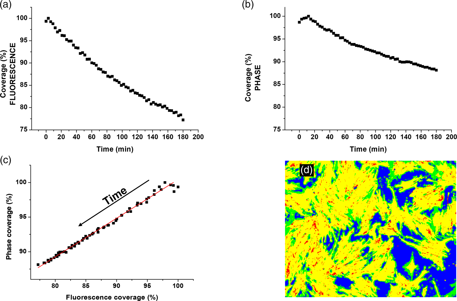
Fig. 4. Cell contraction (shrinking) as a function of time. (a) Fractional area coverage of cells, as detected from fluorescence images. (b) Fractional area coverage of cells, as detected from phase-contrast images. (c) Correlation between fluorescence and phase-contrast detection. The correlation coefficient is r = 0.996. The red line represents a linear regression with a slope of 0.55. (d) Color-coded segmentation parameters of last frame in the time-lapse: yellow – TP, green – FP, Red – FN, and blue – TN.
In Figure 3, we present the simultaneously acquired phase-contrast images, probability images, and segmented probability images of the first and last frames in the time-lapse measurement, respectively. The probability images are the output of the machine-learning classifier. The shrinking of the cells is readily visible. The resulting quantification of the coverage is described in Figure 4b.
At this point, segmentation performance parameters can be calculated, treating the fluorescence-image-derived maps as ground truth, and the phase-contrast-derived maps as the recognition. An overall impression of the performance can be seen in a color-coded map, as shown in Figure 4d. Visually, it is obvious that the phase-contrast-derived maps overestimate the size of the cells (the green areas represent False Positives, i.e., pixels identified as cells, that are in fact background), and obviously under-estimate the background. We report Accuracy = 0.77, Precision = 0.74, and Sensitivity = 0.95. The likely cause for the overestimation of cell sizes lies in the fact that phase contrast creates halos that extend over the edges of the cell; thus, a cell in phase contrast does appear larger than the same membrane-stained cell in fluorescence contrast. This approach is thus not suitable for precise segmentation of cell contours. The performance parameters calculated above indicate a worse performance than much more rigorous approaches (Jaccard et al., Reference Jaccard, Griffin, Keser, Macown, Super, Veraitch and Szita2014), which are aimed at precise segmentation. However, we stress that it is not the performance benchmark we are seeking. Instead, we would like to evaluate the success of our approach to correctly capture the trends in changing coverage. For this purpose, we plot the fluorescence versus phase-contrast area fractions in Figure 4c. In addition to the readily observable excellent correlation, we calculate a Pearson correlation coefficient of r = 0.996 (99% CI: 0.993–0.998, N = 60). We note that on comparing the correlations obtained in all the performed experiments, the value of the correlation did not fall below 0.95, see Table 1.
This indicates that the method described here to quantify changes in the area fraction occupied by cells over time, from phase-contrast images, is in excellent agreement with the fluorescence-image-derived method. We note that the agreement is somewhat lower for coverages between ~98 and 100%, that is, at the initial stages of measurement, when the contraction of cells is just beginning. Additionally, the phase-contrast detection seems to be in general less sensitive than the fluorescence-based detection: according to phase-contrast detection, the contraction of the cells proceeds to ~88% of the original coverage, while according to fluorescence detection it proceeds as low as ~77% by the end of measurement. This fact is also observed in the slope of the linear regression described by the red line in Figure 4c, with a value of 0.55 ± 0.05, which implies that phase-contrast detection is approximately 2 times less sensitive than fluorescence detection. This can be a result of the fact that slight changes in the base of the cell are not easily observed in phase-contrast, as opposed to fluorescence. Also, the optical resolution in phase contrast is lower, due to the reduction of effective N.A. by the phase anulus. Nevertheless, it is very clear that changes in area coverage of cells can be easily monitored using phase-contrast microscopy alone, assisted by an easily trained machine-learning classifier.
An Attractive Application: Growth Curves of Adherent Cells
Growth curves of adherent cells is a highly important parameter, allowing to monitor and handle cell cultures development and for assaying the influence of various drugs on the proliferation rate (Iloki Assanga et al., Reference Iloki Assanga, Gil-Salido, Lewis Luján, Rosas-Durazo, Acosta-Silva, Rivera-Castañeda and Rubio-Pino2013; Jaccard et al., Reference Jaccard, Griffin, Keser, Macown, Super, Veraitch and Szita2014).
To demonstrate the usefulness of this label-free approach to monitoring the area fraction covered by cells, we performed an experiment where we grew MSCs in a nondifferentiation medium and followed the area they covered as a function of time. In general, it is desirable to avoid altering the behavior of cells under study by fluorescently (or otherwise) tagging them. In the case of stem cells, this becomes even more important, since such alterations may lead to fundamental, unintended, biological processes. In our experiment, we followed the cell culture during 7 days from seeding, and quantified the area covered by the cells, according to the approach described above for phase-contrast images. Numerous experiments were performed, with variation in the parameters: different culture dishes, different positions in the same dish, different initial densities of seeded cells, to enable verifying the broad applicability of the conclusions. In the following, we present one typical example.
In Figure 5, we present the original image and machine-learning-based segmentation of the second and last days.

Fig. 5. Proliferation of MSCs monitored during 7 days with phase-contrast microscopy. (a) Phase-contrast image, day 2. (b) Machine-learning-aided segmentation of the image in (a). (c) Phase-contrast image, day 7. (d) Machine-learning-aided segmentation of the image in (c). (e) Fractional area coverage of cells as quantified in each of the 7 days. Red continuous curve is a fit of the data to the Gompertz function of the form  $C = Ae^{{-}e^{{-}k( t-t_0) }}$ with t 0 = 2.26 and k = 1.33 (see text for details).
The relative area coverage extracted from the segmented images is plotted as a function of time in Figure 5e. To demonstrate that the measurement is valid, we fitted the data to a Gompertz function of the form  $C = Ae^{{-}e^{{-}k( t-t_0) }}$, where C is the coverage, A is the upper asymptote (in this normalized case, it was defined as 100% on day 7), k is the rate coefficient, t is time, and t 0 is the time at the inflection point, where the coverage is A/e or 36.8% of the asymptote. The Gompertz model is perhaps the most frequently used sigmoid model fitted to growth data (Tjørve & Tjørve, Reference Tjørve and Tjørve2017). According to the fit, the maximal rate of growth occurs at 2.26 days from start and has a value of 49%/day (of the previous coverage), and a population doubling time of 2.6 days in full agreement with standard growth-curve measurements, obtained by harvesting cells and counting them in a hemocytometer (not shown). The key parameters from this curve are k, the growth rate coefficient, which does not depend on the units of the Y-axis (whether normalized or not, or whether it represents absolute or relative number of cells) and t 0, the inflexion point, or the time point when the growth rate is maximal. The (maximal) rate of growth at the inflection point is given by Ak/e and the population doubling time is given by
 $$t_0-\displaystyle{{\ln( \ln2) } \over k}.$$
Thus, the comparison of k and t 0 between different culture conditions (e.g., various drugs or toxicants), or even different methods of extracting growth curves, is a very powerful research tool. For adherent cells, the traditional measurement of a growth curve is a labor-intensive task, involving harvesting, fixation, and/or staining cells at multiple time points (Iloki Assanga et al., Reference Iloki Assanga, Gil-Salido, Lewis Luján, Rosas-Durazo, Acosta-Silva, Rivera-Castañeda and Rubio-Pino2013). The method described here is fast and user-friendly, noninvasive, and nondestructive.
Simplified Approach to Proliferation Assessment
While the above approach is very advantageous, its drawbacks are that machine-learning algorithms are typically slow, require high computation resources, and demand human intervention during the training process. In this section, we examine whether, for the limited scope of calculating area coverage of freely proliferating cells (no segmentation of individual cells), a simple thresholding of phase-contrast images is sufficient. To elaborate on this approach, we reiterate the fact that, as mentioned in the introduction, threshold-based segmentation in phase-contrast images results typically in segmentation of the halos only, and not the whole cell area. However, if we assume that the area occupied by halos is roughly proportional (but smaller) to the area the whole cell occupies, then quantifying the area covered by cells may be assessed from the area occupied by halos. Of course, the above assumption is not easy to justify: the size and intensity of halos in phase-contrast microscopy is difficult to predict, since it depends on the magnitude of gradients in the index of refraction, and these strongly depend on the (3D) morphology of the cell membrane. Since the morphology is unknown and is not uniform among different cells (some cells are round and small, some are triangular, some are elongated, etc.), this assumption seems unsubstantiated. Nevertheless, upon averaging over a large number of cells in a field-of-view, this approach proves to yield a more predictable value. This is so because the variation in the distribution of cell morphologies between images (taken one day apart) may not be very large, and if this is the case, the relative change in intensity of the halos may be roughly proportional to the number of cells observed in the field of view.
To experimentally test the validity of this assumption, we applied direct thresholding of the same phase-contrast images referred to in Figure 5 and compared the results with the machine-learning segmented images. The original images and the respective segmented halos are shown in Figure 6.

Fig. 6. Proliferation of MSCs monitored during 7 days with phase-contrast microscopy. (a) Phase-contrast image, day 1. (b) Thresholding segmentation of the image in (a). (c) Phase-contrast image, day 7. (d) Thresholding segmentation of the image in (c). (e) Fractional area coverage of cells as quantified in each of the 7 days. Black squares represent results obtained using the machine-learning approach (same data as Fig. 5e), red circles represent results obtained using thresholding, for comparison. (f) The results obtained by the second method (threshold) as a function of those obtained by the machine-learning method. The red line represents a least squares linear fit to the data.
In Figure 6e, we plot the data obtained using the thresholding method, together with the data obtained using the machine-learning method (as described in Fig. 5), for comparison. It is clear that, while there is no perfect overlap, the correlation between the two methods is very strong (Fig. 6f) with a Pearson correlation of r = 0.991 (99% CI: 0.949–0.998, N = 7). Thus, even though the coverage obtained from thresholding obviously does not represent the true area covered by cells (but rather the area covered by the halos), k and t 0 are still valid, since they do not depend on scaling of the Y-axis, and since, as it turns out, in these specific conditions (this type of cells and this range of cell density) the assumption that the area of the halos is proportional to the cell area holds. In Table 2, we report the results obtained for various initial seeding densities, for reference.

Conclusion
While phase-contrast images suffer from well-known artifacts, the phase-contrast microscope is still the most common analytical instrument in a cell-culture facility. Although traditionally it is only used as an inspection tool, we show here that it can be used as a quantitative tool, with the aid of modern, accessible and easy-to-use machine learning software and powerful personal computers.
We described two distinct cases where quantification of the area covered by cells is possible and accurate, providing important biological information in a noninvasive and nondestructive manner.
Case 1: The number of cells in the field of view does not change, however the area of the individual cells is changing, for example, cells that are shrinking in response to a toxic environment. The area fraction occupied by cells may be very useful in assessing toxic effects of a variety of substances, continuously, even if transient. It is worthwhile studying to what extent such approaches can lead to systematic quantification of toxicity, at much more delicate levels than existing assays (most of which include staining and report on very final stages of toxic effects, mostly cell death).
Case 2: The size of the cells in the field of view does not change considerably, however their number is changing, with proliferation being the simplest example we demonstrate (migration in or out of the field of view may serve as another example). It is hard to overestimate the importance of cell growth curves as a research tool, however the methods used for adherent cells are labor-intensive and disruptive, since they involve harvesting (thus destruction of the specific culture) and/or staining, before counting (by a variety of methods). Not only our method allows assessing growth curves of the very same culture, in a label-free manner, but it is also easy to imagine how growth curves in different areas of the same culture may be obtained and compared, thus offering a measure of position-dependent proliferation rates.
In addition, we demonstrate that, if a set of assumptions holds, the relatively computing-intensive machine-learning part may be avoided, and accurate proliferation rates may be obtained from phase-contrast images by traditional and fast methods (direct threshold). We emphasize that the growth curves obtained this way should not be interpreted as “confluency,” since they are only proportional (with an unknown constant, smaller than 1) to the true percentage of the area covered by the cells.
In analyzing growth curves, the key quantitative information is contained in the parameters k and t 0 of the fit to a Gompertz function, and these can safely be compared between different cultures and different methods of obtaining the growth curves, since they do not depend on the scaling of the Y-axis. The ML method overestimates the true area of the cells (as assessed from fluorescence images), but by a constant factor, thus the correlation over time between the two methods is excellent (but not the agreement regarding absolute coverage). The thresholding method under-estimates the true area of the cells (as assessed from ML images), by a constant factor (when the appropriate conditions hold), thus the correlation over time is excellent (but not the agreement regarding absolute coverage). Absolute coverage can still be estimated from the flattening of the growth curve, in all methods of obtaining of growth curves.
It is very important not to use the simple thresholding method in cases where the cells are shrinking (or swelling), like in the first case reported here. In such cases, the assumption “area of halos is proportional to the area of cell” obviously does not hold.
Supplementary material
To view supplementary material for this article, please visit https://doi.org/10.1017/S1431927622000794.
Acknowledgments
We thankfully acknowledge Ms. Nily Ben-Shushan for close technical support, and Prof. Razi Vago's lab members for their help.


 Open access