
Abstract
In this paper the focus is on thermal and electrical design aspects of a NbTi-based demonstrator magnet for magnetic density separation (MDS) that is being constructed at the University of Twente. MDS is a recycling technology that allows the separation of non-magnetic particles based on their mass density, using a vertical magnetic field gradient and a ferrofluid. To minimize the distance between the planar array of racetrack coils and the ferrofluid bath, the system is conduction-cooled. First the thermal design is presented, which shows that the coils can operate below 4.5 K with sufficient margin using a single cryocooler. High-purity aluminium heat drains enable a low thermal gradient across the cold mass. The current path is introduced, as well as the adopted protection scheme. The magnet's stored energy can safely be dumped in the coils. Diodes are placed (anti-)parallel to the coils in the cold to prevent high terminal voltages. In the case of a quench in the superconducting part of the current leads or an external anomaly, a switch is opened and the current is forced through a resistor in series with the diodes, causing a deliberate transition of the coils to the normal state and thus a fast ramp-down.
Export citation and abstract BibTeX RIS

Original content from this work may be used under the terms of the Creative Commons Attribution 4.0 license. Any further distribution of this work must maintain attribution to the author(s) and the title of the work, journal citation and DOI.
1. Introduction
At the University of Twente a demonstrator NbTi/Cu-based magnet for magnetic density separation (MDS) is being constructed. The magnet has to provide a vertical magnetic field gradient in the MDS system. MDS is a recycling technology that allows the separation of non-magnetic materials based on mass density [1–6].
In this process, illustrated in figure 1, shredded feed particles are immersed in a superparamagnetic fluid (ferrofluid), which flows over a magnet. The fluid, consisting of a carrier liquid (usually water) with a concentration of superparamagnetic nanoparticles dispersed in it [7], is magnetized to saturation by a magnet that generates a vertical magnetic field gradient [1]. The magnetized fluid is thus attracted towards the magnet, leading to a net buoyancy force on the non-magnetic feed particles which pushes them up to an equilibrium height that depends on the mass density of the particle. The strength of the magnetic field (gradient) and the ferrofluid concentration can be designed to match the application-specific density range. Different-density particles float at different heights in the fluid bed. The horizontal component of the force on the ferrofluid pushes feed particles towards separator blades that collect the different-density streams. After this, the ferrofluid is recovered and the separated products go through a sensor sorting process for final purification [6]. A transport belt moves over the magnet to carry away any magnetic particles that might be present in the feed stream.

Figure 1. Schematic of an MDS system. Non-magnetic feed particles are immersed in a ferrofluid that is attracted to a magnet. The combination of vertical forces on the feed particles (gravity, buoyancy and effective repulsion by the magnet) dictates the equilibrium height of the particles depending on their mass density. After separation, the particles are collected by a conveyor belt that runs out of the sketched plane. z is the vertical direction.
Download figure:
Standard image High-resolution imageExamples of possible feed streams are mixes of different plastics [2, 3] or municipal waste (which contains among others gold-enriched concentrates that, using MDS, can be separated from other heavy non-ferrous metals such as copper and zinc [4]). The superconducting demonstrator aims to separate materials found in electronics, e.g. shredded motherboards. The NbTi-based system allows a reduction in ferrofluid nanoparticle concentration of around 25%, and an enhancement of separation resolution of a factor 2.5 [8].
The MDS process is cost- and energy efficient compared to alternatives, potentially providing a significant step forward towards a circular use of resources [2, 5]. The major advantage compared to other types of magnetic separation using a ferrofluid is the ability to separate multiple density components in one process step, while the other types of separation are based on a binary sink-float approach [9]. The binary sink-float approach is used for the separation of for example gold [10], diamonds [11] and coal [12]. As with many sustainability-related technologies, superconductors can enhance the performance significantly [13]. For a discussion on the benefits superconducting magnets can bring to MDS compared to the state-of-the-art permanent magnets employed in this technology, the reader is referred to [14].
The three NbTi/Cu-based coils in the MDS demonstrator are racetracks with a width of 0.30 m each, length of 1.4 m and thickness of 50 mm, and are placed adjacent to each other. The peak magnetic field at the full operating current of 300 A is 5.2 T and the average magnetic field magnitude at the bottom of the fluid bed is 2.0 T. The present manuscript focuses on the thermal design of the magnetic system, and on the electrical circuits used to excite and protect it. The electromagnetic design of the magnet is detailed in [8, 14, 15], and the mechanical design in [16].
Figure 2 gives an indication of the geometry of the major components in the system. The design of this magnet involves the minimization of the coil-to-fluid distance so that the magnetic field is utilized to its fullest extent. The large planar surfaces that are formed by the bottom of the ferrofluid bed and the top surface of the coils present a unique minimization challenge that is absent in most other applications of superconducting magnets.
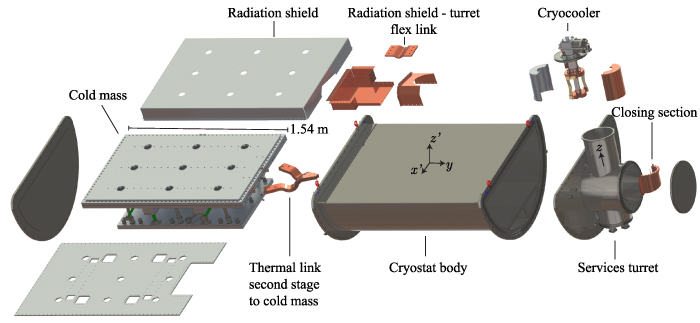
Figure 2. Exploded view of main components of the magnet system. MLI blankets are not shown. z is opposite gravity.
Download figure:
Standard image High-resolution imageAt first, the idea for the demonstrator was to design and build a helium bath-cooled magnet. This would require a double-walled cryostat. The flat top plate(s) of the cryostat needs a significant thickness to resist the combination of the outside pressure and the magnetic force resulting from the ferrofluid-magnet interaction. To maximize the performance, i.e. the vertical gradient of the magnitude of the magnetic field at the fluid bed, the demonstrator design has been optimized to minimize the distance between the coils and the ferrofluid bath (to 50 mm).
As part of this optimization, it was decided to cool the coils via conduction, as this allows the elimination of one cryostat wall. To help minimize the required top-plate thickness, nine stainless steel columns are installed to support the flat top plate. The columns pass through holes in the cold mass and stay at room temperature. The increase in performance of a conduction-cooled single-walled configuration supported with columns relative that of a bath-cooled double-walled option is estimated at a factor 2 [16]. Other advantages are the absence of cryogens and reduced system mass.
The coils need to operate at a temperature T of 4.5 K or lower in order to allow operation with a temperature margin of 2.0 K at full operating current. A procedure that ensures a safe shut-down in the case of an (external) anomaly also needs to be included in the design. In this work these thermal and electrical aspects are dealt with. The layout of the paper is as follows:
- First, a thermal overview of the system is given in section 2. This includes the calculated heat loads at the two stages of the cryocooler and the expected thermal gradient between cryocooler and coils. It is demonstrated that the system is expected to be operable with conduction-cooled with a single cryocooler.
- Second, the layout of the current leads and electrical connections are presented in section 3. The feasibility of the quench protection method for this system is explored, as well as the ability of a fast ramp-down in the case of an external anomaly. This ramp-down can be started by means of a manual trigger or by automatic actuation after detection.
2. Thermal design
This section concerns the thermal design of the magnet. This includes minimizing the heat in-leak from various sources on the cold mass and on the radiation shield, as well as minimizing the temperature difference between the warmest spot in a coil and the second stage of the cryocooler.
The coils are designed to operate with a maximum temperature of 4.5 K, allowing a temperature margin of 2.0 K. Since the cooling power of the cryocooler is temperature dependent, the heat in-leak to the cold mass can not be too high as otherwise the temperature of the second stage of the cooler will be above the acceptable value. This acceptable value is significantly lower than 4.5 K, since a thermal gradient between the coils and the cryocooler is unavoidable.
The cryocooler is a model RDK-415D2 two-stage Gifford-McMahon cooler from Sumitomo Heavy Industries, Ltd The powerful first stage is commonly used to intercept heat coming from room temperature to the cold mass. To intercept radiation from the room-temperature vacuum vessel, a heat shield made from copper and aluminium is placed around the cold mass, the support structure, the current leads and the cryocooler.
Heat transfer due to convection will be regarded as negligible due to the vacuum inside the cryostat. What remain to be considered are radiation and in-leak via conduction, ramping losses in the superconductor, as well as joule heating in resistive parts of the electrical circuit. The next section introduces the components that contribute to a significant heat load into the system.
After the identification of relevant heat loads, a lumped thermal model is solved to find the magnitudes of the heat loads as well as the temperatures of the cryocooler stages, radiation shield and cold mass. The model also allows an estimation of the cool-down time of the system. The cool-down is performed by the cryocooler without the aid of additional cryogens. While using liquid nitrogen to speed up the cool-down process is possible, it was decided not to do so for the demonstrator, in favour of simplicity. For the same reason removable heat-links—high-thermal conductivity links that can be mechanically disconnected at a certain point in time—between the intermediate stage and the cold mass are not considered.
Using the results of the lumped model, an estimate of the thermal gradient in the cold mass is made using a 3D FEM calculation. This allows for a prediction of the warmest spot in the coils.
2.1. Heat loads
Several components that introduce a significant conductive heat in-leak can be distinguished. They are summarized in table 1. These values are derived in the following sections.
Table 1. Heat load overview.
| Heat load type | After cool-down | During magnet ramp |
|---|---|---|
| First stage | (W) | (W) |
| Current leads | 16.8 | 25.2 |
| MLI | 5.7 | 5.7 |
| Support structure | 2.5 | 2.4 |
| Total | 25.0 | 33.3 |
| Second stage | (W) | (W) |
| Current leads | 0.047 | 0.058 |
| Thermal radiation | 0.22 | 0.33 |
| Wiring | 0.005 | 0.005 |
| Total | 0.40 | 0.54 |
A first major source of heat load is the mechanical support structure keeps the cold mass in place within the cryostat. This support structure exhibits the conflicting requirements of low thermal conductance and high mechanical strength. The optimization of the chosen fibreglass structure is described in [16].
It consists of four vertical G11 tubes (9.0 cm2 total cross-sectional area)) and four horizontal G11 rods (12.6 cm2 total cross-sectional area), see figure 3. The pillars are heat-sunk to the cryocooler's first stage via the radiation shield to reduce the in-leak at the cold mass. The attachment to the vertical tubes also supports the weight of the radiation shield. The vertical tubes have an effective length between room-temperature and the intermediate heat-sink of 93 and 113 mm between the heat-sink and the cold mass. For the horizontal rods these lengths are 0.17 and 0.5 m, respectively.

Figure 3. Exploded view of cold mass with radiation shield. MLI blankets not shown.
Download figure:
Standard image High-resolution imageA second major heat-load results from thermal radiation. The inner surface of the cryostat's outer vessel has an area of approximately 5.0 m2, and the radiation shield an area of 4.2 m2. The radiation shield is shown in figure 3.
Copper is used for parts of the radiation shield that see a relatively high heat flux, while aluminium is used for the other parts to reduce weight and costs. The main structural component of the radiation shield consists of a 10 mm plate of AL2024-T351, which is placed below the cold mass. Type of aluminium was chosen because of availability, it has a thermal conductivity at 77 K of 90 W m−1 K−1, which is average compared to other aluminium alloys [17]. The plate is kept in place via the vertical pillar heat-sinks, which are glued to the pillars with Stycast 2850FT. These heat sinks consists of 10 mm thick plates of AL1060 and are connected to the main plate via 2 mm sheets of AL1060.
The top cover of the radiation shield is also made from 2 mm thick AL1060. The connection between parts is with bolts. Threads are vented to prevent the creation of pockets of trapped air during de-pressurisation of the system. The transfer of heat from shield to cryocooler is achieved with copper pieces. Attached to the bottom main plate is a 3 mm thick copper plate section. This section and previously mentioned components are assembled around the cold mass before insertion into the cryostat.
On the top of the cryocooler's first stage a copper hollow cylinder with 10 mm thickness is attached via M6 bolts before mounting the cooler in the cryostat turret. After installation of the coils/cold mass and cooler, the radiation shield is closed by installing a second copper hollow cylinder of 10 mm thickness and two side plates, indicated as 'closing section' in figure 3,
This cylinder is then connected with the copper plate section of the radiation shield via a flexible copper connection, consisting of 155 mm wide, 0.2 mm thick OFHC copper foils that together form a 10 mm thick stack. The two outer end of the foils are press-welded to form solid terminals. In this way, a flexible component is obtained that allows bending in one direction. This movement by bending allows stress-free movement of the cold mass relative to the cryocooler during cool-down. The link is annealed at 300 ∘C for 6 h in a vacuum environment to increase the thermal conductivity.
The radiation shield itself is wrapped in three blankets (consisting of 10 layers each) of MLI made by RUAG Space, with a blanket thickness of 3 mm when uncompressed [18]. As first, the idea was to also include a blanket between the radiation shield and the cold mass. However, this idea was later disregarded. The heat load on the cold mass through a 3 mm blanket of MLI from 65 K to the cold mass is estimated at around 0.17 W m−2 [19]. However, this value depends strongly on layer density N ( [19]), so any compression applied while installing the 3 mm blanket in the 4 mm clearance that is available will rapidly increase the heat load. With a shield temperature of 65 K, the radiative load obtained by omitting the MLI will be of a smaller value as long as the emissivity is lower than 0.16. This is thought to be achievable: Iwasa, for example, lists values for 80 to 4 K plates of 0.02 and 0.06 for mechanically polished copper and aluminium respectively [20]. We will assume a value of 0.1 in the rest of this work.
Another major source of heat comes from the current leads of the coils. These current leads are divided into two distinct sections. The operating current of the magnet of 300 A is fed from room temperature to the thermalization point on the cryocooler's first stage via copper current leads with RRR 30. The transfer of the current from the first stage to the second stage is achieved via BSCCO-2223 current leads made from Sumitomo type G conductor. The superconducting section has a silver-gold alloy matrix for its reduced thermal conductivity relative to a pure-metal matrix [21]. Each leads consists of three tapes with a length of 0.16 m each and a cross-sectional area per tape of 4.3 mm by 0.23 mm. Additionally, the tapes are mechanically supported by a 2 mm thick G11 sheet per lead.
The BSSCO tapes have a critical current  per tape at self-field of 291 A at 66 K. They are situated in a low-field region (
 100 mT), thus no strong correction is needed because of the background magnetic field [21]. This yields a margin of a factor 3 in
  when the leads are anchored to the second stage at 66 K.
Part of the current leads are shown in figure 4. One can see the vacuum feed-throughs with a relatively large cross-sectional area to make sure the vacuum seals are at room-temperature. Also shown are the heat-sinks to the first- and second stages, and the superconducting connection between the two stages. The copper connection between the vacuum feed-through and the first stage heat sink is not shown. The current flows from the vacuum feed-through to the not-shown copper current lead via a soldered connection. A close-up of the first stage is shown in figure 5.
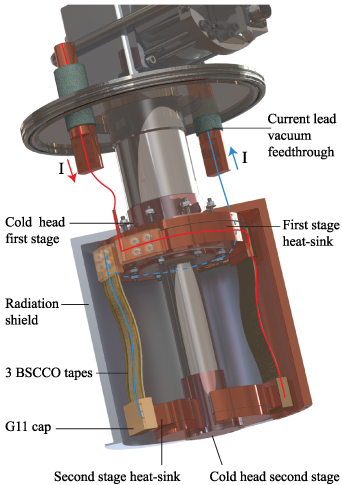
Figure 4. Current leads and heat-sink. The current path going in and out of the set-up is sketched in red and blue.
Download figure:
Standard image High-resolution image
Figure 5. View of the first-stage heat-sink. Not shown are the connections between the vacuum feed-through and the copper rod, G11 insulation caps and the MLI layer.
Download figure:
Standard image High-resolution imageThe lead is soldered to a copper rod and copper plate combination. This plate is bolted to the heat-sink with an indium foil in between. The heat-sink consists of a copper main ring, making contact with the cryocooler flange. A second, C-shaped, piece of copper is glued to this ring. G11 insulation pieces of 0.2 mm thickness provide electrical isolation. The current flows through the C-shaped part, thus maximizing the thermal contact area with the first-stage heat-sink. At the other end of the C, the superconducting lead is bolted using a copper plate-indium-copper connection. G11 caps are placed over several areas over the current leads to prevent electrical contact with the MLI layer. Other parts are wrapped in Kapton foil.
The second stage heat-sink is similar to that of the first stage. The current is passed from the second stage heat-sink to the coils using NbTi/Cu conductor. Four wires with the same properties as that of the winding packs (diameter 1.44 mm) are placed in parallel to form a lead. Using four conductors instead of a single conductor increases the current sharing temperature of this section from 6.5 K to 6.8 K. This gain is small because of the steep drop of performance of NbTi with increasing temperature.
For the first stage heat-sink the contact area between the copper ring and the copper C-piece is 92 cm2. Using a thermal conductivity of G11 of 0.28 W m−1 K−1 at 77 K [22] and a heat load of 12.6 W per lead (as calculated in the next section), a temperature difference between the two copper pieces of around 1 K is expected.
The second stage heat-sink has a contact area of 59 cm2. With a heat load of 32 mW per lead, this gives a gradient of 15 mK across the G11 (k of 0.072 W m−1 K−1 at 4.2 K [22]) and 11 mK across the two Stycast interfaces (k of 0.05 W m−1 K−1 at 4.2 K [22]). The thermal contact resistance across these interfaces is expected to be below 1 mK [23].
The wiring connecting the various sensors to the read-out instrumentation carries in a small amount of heat to the cold mass, estimated at 5 mW. As this is a demonstrator system, a larger number of sensors is desired than one might consider for a production model. In the rest of the paper we will omit this small heat load.
The hysteresis loss rate Physt—the power dissipated by movement of fluxoids in the superconductor due to a changing magnetic field—is estimated, from [24], by integrating the product of the rate of change of the magnetic flux density,  , and critical current density
  :
:
where λsc is the volumetric fraction of superconductor in the winding pack (29%), Vwindingpacks the volume of the three winding packs (42 L) and dfil the diameter of the superconducting filaments (75 µm).
The effect of transport current on the dissipation is neglected as the ratio between the current density and critical current density is low ( 20%).
20%).
From the calculations, it seems realistic to use 0.1 W as a heat load for the hysteresis loss for a 15 h ramp. The effect of ramping at a higher speed is discussed in section 2.3.
The relative contributions of eddy currents and coupling losses to the heat load during ramping are small compared to that of hysteresis.
It is of interest to find out at which temperatures of the first and second stages of the cooler the cooling power will equal the heat load at these two stages. The next section concerns a lumped thermal network that solves the heat loads and temperatures.
2.2. Lumped thermal model
A lumped thermal model is used to calculate the temperatures and heat flows in the system. To calculate the temperature at which the heat loads on the first and second stages of the cryocooler balance the cooling power, the cooling power as a function of temperature is required as an input. Measured data presented in [25] are used, as they are more detailed than the official load-map [26]. The low-temperature measurement points are shown in figure 6. This paper also includes data on the second stage cooling power up to 16 K [25].

Figure 6. Cooling power of RDK-415D cryocooler as a function of temperature and load at neighbouring stage. Data are taken from [25]. Also indicated are the expected operating points of the MDS demonstrator magnet system as calculated using the lumped thermal model.
Download figure:
Standard image High-resolution imageAdditionally, a data-point at 150 K is taken from [27]. At this temperature, the first stage was measured to have a cooling power of 80 W and the second stage of 45 W, measured using 60 Hz input power. In the lumped thermal model, the interpolation between data-points is set to linear and extrapolation to constant. In this way, the cooling power above 150 K is thought to be underestimated. The performance differences between 50 and 60 Hz input power are acceptable for our use of these high-temperature data-points, which is a calculation of the cool-down time of the system.
The lumped thermal network consists of thermal masses connected via conductive links, as shown in figure 7.
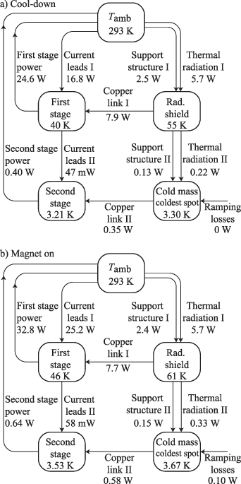
Figure 7. Heat flows and temperatures in lumped thermal network calculations: (a) situation after cool-down and (b) effect of ramping up the magnetic field.
Download figure:
Standard image High-resolution imageThe considered masses are the first and second stages of the cryocooler, radiation shield and cold mass. The cold mass is considered to be at a uniform temperature; the gradient across the cold mass is subject of the next section.
The first stage is connected to a fixed room temperature node via the current leads. The current leads also connect the first and second stages. The thermal gradients between current leads and cryocooler, estimated earlier in this work at 1.0 K for the first stage and 26 mK for the second stage, are neglected here.
The radiation shield is connected to the cryocooler via a copper link (Copper link I in the figure). This link represents the copper link as a resistor in series with a second resistor representing the gradient across the shield. The warmest point on the shield is used to calculate heat transfer from and to the shield. This includes heat flow through the fibreglass support structure to the shield from room temperature (Support structure I) and from shield to cold mass (Support structure II). The effective thermal resistance of the shield in Copper link I is matched so that the calculated hot-spot temperature matches results from a 3D FEM calculation of the radiation shield, which will be shown later.
The second stage of the cryocooler is connected to the cold mass via a thermal link. This link consist of copper OFHC laminates. These are hot-pressed at their ends to form solid end-pieces, similar to the link discussed for the radiation shield. The effective cross-sectional area is 45 cm2. The flexibility resulting from a bend in the laminates allows for a stress-free cool-down of the system. The RRR of the thermal links in the calculations was set to 100, a low-end value for annealed OFHC copper [22].
This link connecting the cold mass and the cooler consists of two copper parts, which when installed make up the shape of a letter V, as can be seen in figure 3. Here the bottom of the V corresponds to the anchoring points on the cold head. This solution is chosen as it allows a connection on the cold mass on two places between the racetrack coils, where there is space to bolt the link (via a 100 µm thin indium interface) with sufficient force (60 kN per link). Titanium bushings are used to prevent the pre-tension being lost on cool-down. The path-length between the middle of the cold contact area and the middle of the warm contact area of the link is taken as the effective length over which the gradient is calculated. This length is 30 cm.
Due to the relatively small contact area between cold head and thermal link, the interface between the two must be carefully considered as thermal contact resistance at low temperatures can be significant [22]. The copper link is connected to the cryocooler's second stage using six M6 bolts and a pre-tension of 7 kN each. The thermal contact resistance is included twice in the model, in series with the V-link. The interface material is a 100 µm thin layer of indium, with thermal contact resistance data from [28].
The copper V-link is situated partly in a medium magnetic field region (up to 2 T). The reduction in thermal conductivity due to the magnetic field is around 13 .
.
The calculated temperatures and heat flows are given in figure 7. The second stage cools down to 3.2 K and increases to 3.5K when the magnet is ramped up. The first stage cools down to 40 K and increases to 46 K when the magnet is powered. The cold mass eventually cools to a temperature of 3.3 K at the point where the thermal link is attached.
The heat load through the copper current leads is calculated using a 1D FEM model. When carrying current between 293 K and 46 K, the optimal cross-sectional area per lead for copper with a RRR of 30 was found to be 76 mm2 per meter of length.
A simplified 3D FEM calculation representing the aluminium AL2024-T351 bottom plate of the heat shield and AL1060 top cover was performed to estimate the temperature gradient across the radiation shield, see figure 8. The thermal conductivity of AL2024-T351 and AL1060 was taken from [17]. The applied heat loads are those of radiation and anchoring of support pillars as calculated in the lumped model, see figure 7.

Figure 8. Temperature distribution in the radiation shield when the magnet has been energized.
Download figure:
Standard image High-resolution imageThe connection to the copper parts is modelled as a small surface with a fixed temperature of 50.5 K (an estimated 4.5 K gradient is present between the cold head and this surface). The result of the simulation is that the warmest spot of the radiation shield is 61.2 K.
The hot-spot temperature of 61.2 K matches the lumped thermal model calculation because the value of the resistor representing the gradient across the radiation shield was chosen to match the 3D simulation result. The temperature of the radiation shield is important for the radiation towards the cold mass, as there is a T4 scaling in the heat flux. Thus the question arises whether representing the radiation shield temperature with a single scalar in the lumped model is valid.
To answer this question a histogram of the temperature distribution of the inside surfaces of the radiation shield is shown in figure 9. The histogram is weighted by multiplying the y-axis by a factor T4. A major fraction of the radiation comes from around 60.8 K, close to the maximum shield temperature.
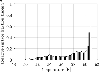
Figure 9. Histogram of inner surface of radiation shield after magnet energizing. The y-axis has been multiplied by T4 to indicate the relative importance of each temperature in the radiative load. The y-axis is normalized.
Download figure:
Standard image High-resolution image2.3. Cold mass temperature
Each coil mainly consists of a stainless steel mandrel, winding pack, two copper spacers and two copper end pieces. The coils are enclosed in two machined aluminium alloy (AL5083-H321) plates that are bolted together. These provide a pre-compression on the winding packs during cool-down due to differential thermal contraction and react to the Lorentz force when the magnet is energized. High purity (RRR 1500) aluminium heat drain bars are present underneath the bottom aluminium alloy plate to reduce the thermal gradient across the coils. These components together make up the bulk of the cold mass, and are presented in figure 10.

Figure 10. (a) Geometry used in the thermal model of the cold mass under normal operation. (b) Same geometry, with the aluminium alloy cassette hidden for clarity.
Download figure:
Standard image High-resolution imageThe winding packs are modelled as orthotropic homogeneous objects. The material properties are calculated using a winding pack composition and with thermal properties as presented in table 2.
Table 2. Thermal conductivity of winding pack components at 4.2 K.
| Material | Thermal conductivity (W m−1 K−1) | Volume fraction |
|---|---|---|
| Copper RRR 100 | 381 at 2.5 T [29] | 0.39 |
| Stycast 2850FT | 0.05 [30] | 0.25 |
| Formvar | 0.011 [31] | 0.075 |
| NbTi | 0.17 [20] | 0.29 |
Data for Formvar, Stycast and NbTi at 4.2 K are used. The thermal conductivity of the winding pack in the direction of the current flow is taken to be a factor 0.39 of that of copper with RRR 100 at 4.2 K. This is because the copper occupies an estimated 39 of the winding pack volume, and because the heat flux in the direction of the conductor can be considered to flow only in the copper, since it has a much higher conductivity than the other components of the winding pack. The effect of magnetic field on the thermal conductivity is taken into account by giving the simulation access to the 3D magnetic field distribution. The measured RRR of the actual conductor is 110. The thermal conductivity of copper as a function of RRR, magnetic field and temperature is taken from [29].
The thermal conductivity perpendicular to the coil turns is estimated by a 2D simulation in COMSOL using a unit cell model. The resulting effective thermal conductivity at 4.2 K is 0.15 W m−1 K−1. This is larger than the 0.07 W m−1 K−1 predicted by the inverse rule of mixtures. The reason behind the difference is that the inverse rule of mixtures assumes that the heat flow has to go through each component in series, whereas in reality the path is partly parallel as well. The value obtained from the simulation was chosen for further calculations.
The thermal conductivity of copper was set to 381 W m−1 K−1 in the calculation of the transverse conductivity, corresponding to a magnetic field of 2.5 T and 4.2 K [29]. This 2.5 T is the mean magnetic field in the winding pack. Thus unlike the longitudinal thermal conductivity, the perpendicular components do not vary with spatial coordinates in the simulation. The results in the perpendicular direction do not change significantly when the magnetic field is changed, since the effective thermal conductivity is dominated largely by the epoxy. The orthotropic material properties of the winding pack are applied via a curvilinear coordinate system.
The thermal conductivity from the high-purity aluminium heat drains takes into account the magnetic field profile, RRR and temperature and is taken from CryoComp [32].
The applied boundary loads in the simulation are:
- a radiative heat load of 303 mW. This load is distributed over all external surfaces;
- ramp loss in the winding packs. A value of 0.1 W is set as a body load on the three coils. This load represents the ramping of the magnet;
- a boundary load of 110 mW is applied representing the in-leak via the vertical pillars;
- similarly a load of 34 mW represents the horizontal pillars.
The connection between the coils and the top aluminium plate is simulated using a 2 mm thick layer of G11, with thermal conductivity of 0.072 W m−1 K−1 [22]. This represents the G11 side-plate of the coils. Likewise the bottom aluminium plate and the coils make contact via a 0.5 mm thick G11 plate. The effective contact area is set to 10% to represent poor contact as it is not sure that the clamping of these surfaces with bolts is effective to establish a large fraction of contact area. The high-purity aluminium heat-drain bars make contact with the aluminium alloy bottom plate and with each other via a Stycast layer of 50 µm thickness. The effective contact area is set to 50%. The same applies to the connection between the coils themselves and between the sides of the coils and the cassette.
The results from the simulation are shown in figure 11. The maximum temperature in the winding pack is 3.85 K and is located near the anchoring areas of the pillar structure. The middle coil is warmest as it is furthest away from the high-purity heat drain bars, indicating that the placement of these bars is not optimal.
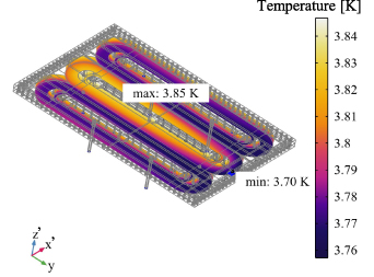
Figure 11. Temperature distribution in coils calculated in COMSOL. Heat loads are applied as detailed in figure 7, representing normal operating conditions. The coldest spot in the cold mass is fixed to 3.0 K and the heat loads are applied as detailed in the main text. The warmest spot in the winding pack is less than 0.1 K above the coldest point.
Download figure:
Standard image High-resolution imageThe coils are designed for stable operation from a superconducting point of view, at a temperature of no more than 4.5 K. This way a 2 K temperature margin with the current sharing temperature is achieved. The calculated 3.85 K maximum is thus below the demand put on the thermal design by the electromagnetic design. One could use the margin in the thermal design to ramp the magnet at a higher rate than the 15 h used in the calculations.
2.4. Cool-down time
As the coils need to be cooled from room temperature to operating temperatures by the cryocooler via a link, it is important that this link has a high thermal conductivity over a wide range of temperatures. Otherwise, the cold head of the cooler could already cool down to a low temperature itself, while the coils are still much warmer. The result is that the cooling power is decreased. For this reason a helium-based heat-pipe is not considered, since the operating range is too narrow [33]. Instead copper and aluminium links as discussed in the previous section are relied upon to transfer heat.
The lumped thermal model introduced in section 2.2 is used to calculate the temperature of the cold mass as a function of time. The mass of components in the calculation is given in table 3. The specific heat as a function of temperature is based on data between 4 K and 300 K from [22]. Extrapolation below 4.2 K is set to linear 1 .
Table 3. Mass of major components in the system.
| Section | Material | Mass (kg) |
|---|---|---|
| Cold mass | Copper | 202 |
| Stainless steel | 92 | |
| Aluminium | 137 | |
| Stycast 2850FT | 33 | |
| Niobium | 52 | |
| Titanium | 27 | |
| Radiation shield | Copper | 27 |
| Aluminium | 55 | |
| First stage cryocooler | Copper | 4.7 |
| Second stage cryocooler | Copper | 3.2 |
The result is shown in figure 12. The first stage of the cooler cools down within a couple h, and a large temperature gradient between it and the radiation shield is present during cool-down. The cold mass takes 12 d to reach a stable temperature of 3.3 K. Here the reader is reminded that the cooling power between 150 K and room temperature is given a pessimistic value, as introduced in section 2.2. As a rule of thumb, this cryocooler takes around 1 h to cool-down 1.5 kg of copper from room temperature to around 4 K [34]. This would yield a cool-down time of 15 d if the entire cold-mass were copper, close to the obtained results.

Figure 12. Cool-down temperature as a function of time calculated using the lumped thermal model introduced in section 2.2.
Download figure:
Standard image High-resolution imageThe temperature difference between the second stage and the cold mass stays small over the cool-down period. Thus the thermal link is found to be adequate.
In the simulation, the magnet is ramped up to 300 A in 24 h, starting at 19 d after the cryocooler is turned on. The major effect of the ramp on the temperature profile is in an increase of the first stage temperature due to the Joule heating in the copper sections of the current leads.
As explained in the next section, the cold mass is expected to warm up to around 100 K after a quench. It can be seen from figure 12 that it would take the system around 3 d to cool down and recover after a quench.
3. Electrical circuit
This section details the electrical circuit of the demonstrator magnet, including current leads and protection circuit.
3.1. Self-inductance and stored energy
The magnet has a total self-inductance of 16.4 H. This is built up from the self-inductance of each coil Li and their mutual inductances Mij . The values are listed in the matrix in equation (2):
Here coil 2 is the middle coil, as indicated in figure 13. The geometry of the coils is derived in [8, 14].
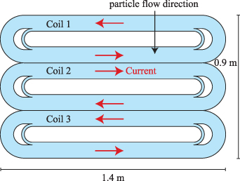
Figure 13. Flow of current in MDS coils, indicated by red arrows. The current direction in adjoining racetrack legs is the same.
Download figure:
Standard image High-resolution imageWith the operating current of the magnet of 300 A, this leads to a stored magnetic energy 2 of 0.74 MJ.
Safely depositing this energy in a short time is required in three different scenarios: (1) a quench in the coils, (2) a quench in the current leads and (3) an external emergency situation requiring a fast ramp-down of the magnetic field.
The mass of one winding pack is 86 kg. This means that if all the stored magnetic energy were to be deposited in a single winding pack, the average heat supplied would be 8.7 kJ kg−1. This would heat the winding pack to around 107 K, whereas a maximum temperature of 150 K is generally accepted [20]. This 107 K is calculated using temperature dependent heat capacities from [22]. The density of the winding pack is estimated using the rule of mixtures based on data from [22] and is set to 6132 kg m−3.
In reality a quenching coil would likely transfer enough energy to a neighbouring coil, causing it to quench as well and distributing the stored energy more evenly.
Thus it seems plausible to use a quench protection method where the stored magnetic energy is mainly dissipated in the coils. This is a common quench protection system for low-field superconducting magnets [20, 24]. It has the benefits of being passive and, when diodes are placed parallel to the coils, of not creating high external voltages. In this section first the adopted electrical scheme is introduced, followed by estimates of hot-spot temperatures in coils and the current leads, ramp-down time, voltages and dynamic mechanical forces.
3.2. MDS magnet's electrical circuit
The electrical circuit of the MDS magnet is shown in figure 14.

Figure 14. MDS magnet's electrical circuit.
Download figure:
Standard image High-resolution imageAs mentioned, the three coils are connected in series. During normal operation the current flows from the power supply through a closed switch, vacuum feed-through (C1+), copper current lead (A2+), copper heat exchanger (HX1+) with the first stage of the cryocooler, high-temperature superconductor (C3+), heat exchanger with the second stage of the cryocooler (HX2+), quad NbTi conductor and finally to the coils.
Connected in parallel to the coils are four diodes. Two of these are connected in forward and two in backward direction. These diodes of the Schottky type are located on the cold mass. By placing them in the cold, no additional warm-cold connections are needed. They are rated to handle up to 600 A continuously at room temperature.
The forward voltage of the diodes was measured in a liquid helium bath, and was found to be 2.01 V at 3.5 A and 1.60 V at 300 A. This drop at higher currents is due to heating of the diode. The diodes limit the ramp-rate of the magnet. If it would be desired to ramp at a higher rate, more diodes can be included.
The reason that the diodes are placed parallel to the combination of three coils in series, instead of placing a diode pair across each coil, is that in the selected configuration each coil always carries the same current. In this way a scenario in which one or two coils carry current while another coil is already ramping down is avoided. This keeps the system simpler as it requires less components and connections. Also, it avoids asymmetric forces and local stress.
The voltage tap locations are shown in the schematic. Two pairs are used for quench detection: V5 + V10 and V6 + V1. This way, a quench originating in the superconducting part of the current leads can be detected as well.
In the case of an emergency, the quench detection system opens the electrical circuit by means of a relay, and the current will flow through the diodes. Also present in series with the diodes is a 10 mΩ resistor. This resistor is a steel slab that is glued to the bottom of the cassette. The aim of this resistor is to cause a quench in the coils when the relay has been opened. It might be possible that the dissipation in the diodes is sufficient by itself to cause a quench in this situation, however, the thermal contact between the current-carrying part of the diodes and the cassette is undetermined. Thus the resistor is added. By causing an intentional quench when the relay is opened, a fast ramp-down of the magnet can be achieved in the case of an emergency in the industrial operating environment. The time-scale of the ramp-down is around 2–3 s, as explored further on in this work.
The current leads consist of copper parts to carry current between room temperature and the first stage of the cryocooler. These are represented in the diagram as A2 and are heat-sunk at HX1. From the first stage of the cryocooler to the second stage three BSCCO-2223 tapes (Sumitomo type G) per lead are present with specifics as detailed in section 2.
If a single one of these tapes transitions to the normal state, the other two tapes in the lead are able to carry the transport current while remaining superconductive as there is enough margin. A possible failure scenario causing all three tapes in a lead to quench is a temperature rise of the first stage of the cryocooler. In principal this temperature rise can be used as a warning, and the magnet can be ramped down by the power supply [35].
However, it is important to make sure that the BSCCO tapes do not burn out in the case a quench, perhaps initiated by another source, does occur and the metal matrix needs to conduct the transport current for a short period.
To get an estimate of what time is allowed to detect a quench and open the switch, a 1D FEM calculation is performed in COMSOL of the BSSCO tapes. The simulation is a coupled adiabatic heat transfer and electrical currents calculation.
The specific heat, thermal conductivity and electrical resistance (at zero external magnetic field) of the tape are taken from the Sumitomo data sheet [21]. The mass density is set to 9.3 g cm−3, based on an estimated composition of 70% silver (10.5 g cm−3 [22]) and 30% BSCCO filaments (6.4 g cm−3 [36]).
The tapes are considered to be thermally isolated from their G11 backbone and it is assumed that no heat can leak towards the cryocooler.
The maximum temperature after 0.6 s is around 200 K. This is considered to be the maximum allowed temperature. Taking into account a switching time of the relay of 0.1 s, this leaves 0.5 s to detect and react on a quench signal. This is thought to be sufficient time.
3.3. Simulation of a quenching coil
A straightforward calculation as presented in section 3.1 resulted in an estimated temperature of a thermally isolated coil during a quench of 107 K. Here it was assumed that the dissipated energy is distributed uniformly. However, as was calculated in section 2.3, the effective thermal conductivity at 4 K of the winding pack perpendicular to the turns is a factor thousand less than along the conductor. Thus it is of interest to find out how this anisotropy influences the hot-spot temperature during a quench.
A quench simulation was performed in COMSOL to determine:
- the maximum temperature in the winding pack during a quench;
- the maximum voltage within the winding pack;
- the feasibility of quenching the coil on purpose in the case of a trigger by the emergency switch to enforce a rapid ramp-down;
- the dynamic force on the high-purity aluminium heat drains, due to induced currents. This is of interest because it allows an estimate whether simply gluing the bars to the cassette provides sufficient strength.
The simulation allows for heat exchange with the cold mass and for induction of eddy currents.
The winding pack is considered to be a homogeneous composite with orthotropic material properties. The winding pack can exchange heat with the steel yoke, aluminium cassette and copper end-pieces, see figure 15. The two outside coils are not included in the thermal calculation, since it was thought that the hot-spot would be higher when assuming that only the middle coil quenches. In reality the middle coil would likely quickly transfer enough energy to the outer coils to make these quench as well. Thus the selected scenario can be regarded as a worst-case as far as the hot-spot temperature is concerned.

Figure 15. Simulation geometry for thermal calculations, consisting of a half of the simplified cold mass, viewed from the bottom. The left image shows the full simulation geometry, and the right image has one of the two parts that make up the aluminium alloy cassette removed to enable a clearer view. One can see the steel yokes and one winding pack. Also shown are copper crescents and end-pieces. Underneath the cassette high-purity aluminium heat drains are present. The dump resistor which acts as a heater to initiate a quench is located on one end of the cold mass. The objects are coloured based on the logarithm of their effective thermal conductivity at 4.5 K and full operating magnetic field.
Download figure:
Standard image High-resolution imageA steel heater of 10 mΩ placed underneath the cassette is activated with the goal of invoking a quench on purpose, for example when an emergency switch is pressed by the operator. By putting the resistor in series with the diodes, see figure 14, no separate current leads for the heater are required, and the heater is activated automatically by opening the switch in the main current loop. The steel heater is placed below one of the heads of the middle coil. In this way, the simulation geometry can be halved because of symmetry. In reality it is probably better to put the heater below one of the straight sections of the centre coil, further away from the copper parts of the coil. In the simulation, the heater starts carrying the operating current after 50 ms. The interfaces between different components are modelled as a 100 µm layer of Stycast 2850FT.
The simulation consists of a coupled magnetic field, electric circuit and heat transfer time-dependent calculation. The electrical circuit is represented by a lumped system consisting of a 10 mΩ resistor Rdump, representing the steel strip, in series with the coils. The coils are represented by a resistance Rcoil in series with an inductance Lmagnet. The self-inductance of each coil and their mutual inductances, as listed in section 3.1, are lumped into one self-inductance Lmagnet. This is correct since each coil carries the same current.
As only a single one of the three coils is assumed to quench, and the other coils remain superconducting during the whole considered time-frame, this coil is the sole contributor to Rcoil. Rcoil is calculated at each time step using the temperature- and magnetic field dependent average resistivity of the conductor,  via:
via:
where Acu is the cross-sectional area of the copper matrix in the wire of 0.84 mm2 and lwire is the length of conductor in the winding pack of 6.3 km. The average resistivity is calculated by:

where Vwindingpack is the volume of the winding pack and ρ is the resistivity of copper with RRR 100, taken from [29]. T and B both vary with spatial coordinates and time. θ is a smoothed Heaviside step function that provides a simplified representation of the superconducting-normal transition. It is zero below 6 K and one above 7 K. Thus regions below 6 K do not contribute to the resistivity. As the quench propagation itself is not a major focus point of the simulation, this simplification of the actual magnetic field dependent superconducting properties is thought to be sufficient.
The magnetic field is calculated at each time step. The geometry used is the same as that for the thermal calculation, with the difference that the outside coils are also included as well as the addition of an air domain.
The resistivity of the copper matrix is used in combination with the current derived from the lumped electrical network to determine the local dissipation P, in W m−3, in the winding pack:
The specific heat of the winding pack as a function of temperature is calculated using the rule of mixtures using data from [22]. For NbTi the heat capacity at zero magnetic field is used. As there is only a difference in specific heat at low temperatures ( 10 K), and the specific heat is small at those temperatures, this is not thought to influence the results significantly.
The orthotropic thermal conductivity in the winding pack is taken into account by introducing a curvilinear coordinate system. In the longitudinal direction the thermal conductivity is set to 38.8 of that of RRR 100 copper. This corresponds to the copper volume fraction in the winding pack volume. The thermal conductivity perpendicular to the windings is set to 0.15 W m−1 K−1 at 4.5 K as determined in section 2.3 and is given the temperature dependence of thermal conductivity of Stycast 2850FT [37].
The heat loads during normal operation are omitted from the simulation, since they are a factor 105 smaller than the dissipation inside the winding pack. The diodes are also not included in the model, as their highly non-linear characteristics required unacceptable calculation times. The effect of this on the simulation results is small, since the diodes would dissipate only a fraction of the total dissipated energy.
As for the results, the temperature profile of the winding pack at selected time-steps is presented in figure 16. The maximum and minimum temperatures of the winding pack are shown in figure 17(a) as a function of time. The coil starts to quench at around 90 ms, 40 ms after the heater is powered on, and the whole winding pack is in the normal state after 130 ms. This corresponds to a longitudinal quench propagation velocity of around 35 m s−1, which is a realistic value for NbTi/Cu conductor [24].

Figure 16. Temperature profile of quenching coil at selected times. The quench is initiated by a heater, which is shown in figure 15. The transition between the normal- and superconducting states is indicated by a red border. The coil is viewed from the bottom.
Download figure:
Standard image High-resolution image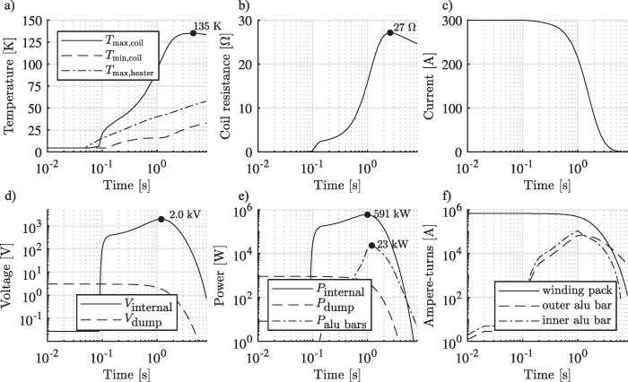
Figure 17. Results as a function of time are shown of calculations for a quenching winding pack that is thermally connected to the cold mass. (a) Temperature inside the winding pack and heater. (b) Resistance of the coil. (c) Current in the circuit. (d) Voltage, inside the winding pack and across the dump resistor. (e) Dissipation inside the winding pack, in the dump resistor, and in the high-purity aluminium heat drains. (f) Ampere-turns in the winding pack and the high-purity aluminium bars.
Download figure:
Standard image High-resolution image
The maximum temperature of 135 K is acceptable. The boundaries of the winding pack are effectively cooled by the surrounding cold mass, which has a relatively good thermal conductivity compared to that of the winding pack in the direction perpendicular to the windings. As a result, only the inner bulk of the winding pack dissipates significant heat.
The steel heater does not overheat, see figure 17(a), thus simply gluing the heater to the aluminium cassette seems a good solution.
The computed resistance is shown in figure 17(b). The resistance climbs up to a value of 27 Ω and then slowly decreases.
This resistance is much higher than that of the 10 mΩ dump resistor, and thus the current, presented in figure 17(c), starts to decay significantly only when the resistance of the coil starts to increase. After three seconds the current is below 5 A.
The maximum voltage occurs inside the winding pack, where the inductive and resistive voltages are opposed to each other. The maximum calculated internal voltage is around 2.0 kV, see figure 17(d). In the considered scenario, in which the middle coil quenches but the two coils on each side remain superconducting, this voltage would be present between the current leads of the middle coil. However, as the coils touch their neighbours over a wide contact area, it is likely that a quenching coil will quickly drive its neighbours normal as well, and thus this internal voltage can be kept lower.
As the simulation allows for the induction of eddy currents, it is interesting to see the magnitude of the currents flowing in the high-purity aluminium bars. Integrating the current density over an  -cross section at the y-symmetry plane of the coils yields the ampere-turns versus time, shown in figure 17(f). The peak current flowing in the aluminium bars is significant compared to that of the coils (up to 23%). However, since the electrical resistivity of the high-purity aluminium (RRR 1500) is much lower than that of the copper matrix of the conductor (RRR 100), the relative contribution to the dissipated power is 4% at maximum, see figure 17(e).
The calculated dissipation is 742 kJ is the winding pack, 24 kJ in the heat-drain bars, 1 kJ in the heater and 7 kJ in the copper end-pieces and crescents and is a result of the fact that the eddy currents are not included in the electrical network. As a consequence, the current in the coils decays at a lower rate than if these effects were included, causing extra dissipation in the system. Thus, the results are interpreted as a worst-case scenario. The diodes, which are part of the protection scheme but not included in this calculation, would each dissipate roughly half that of the heater. The effect of neglecting the diodes on the energy dissipated in the winding pack thus seems small.
From the induced current density in the high-purity aluminium heat drain bars and the magnetic field, the dynamic Lorentz force on these bars can be calculated by integration. The maximum horizontal force on the outer heat-drain bar is 105 kN, pointing outwards. For the inner bar the maximum horizontal force has the same magnitude, directed inwards. This results in a shear stress of 2 MPa on the epoxy connection between the bars and the cold mass, which is acceptable.
From the calculations regarding the quenching of a winding pack thermally connected to the cold mass, it can be concluded that the hot-spot temperature is acceptable when the stored energy is largely dissipated within the winding pack. Also, using a steel heater to initiate a quench to obtain a fast ramp-down in the case of an external anomaly or a quench in the current leads is possible, as the ramp-down time, hot-spot temperature of various components and dynamic forces are at acceptable levels. Thus a protection strategy based on dissipation of the stored magnetic energy in the winding pack is feasible for this magnet.
4. Conclusion
The paper dealt with the thermal and electrical design of the conduction-cooled NbTi MDS demonstrator magnet. The simulations involving the thermal budget of the system show that the magnet can be operated using a single cryocooler. The ability of the system to run conduction-cooled is beneficial for the performance as it avoids the need of a double-walled cryostat. Cool-down is possible in 12 d.
Calculations show that the cold mass is expected to stay below 3.9 K during a 15 h ramp, below the 4.5 K limit imposed by stability- and thermal margin requirements of the superconductor.
The coils are protected by diodes placed on the cold mass. These limit the voltage across the coils' terminals. The maximum internal voltage is 2 kV. The stored magnetic energy of 0.74 MJ is deposited largely in the winding pack itself during a quench, reaching a rather safe hot-spot temperature of 135 K. In the case of an external anomaly or a quench in the current leads, a heater on the cold mass can ensure a fast ramp-down of the system in around 3 s. After a quench the cold mass takes 3 d to cool down to the operating temperature again.
Data availability statement
No new data were created or analysed in this study.
Acknowledgments
This research is part of the programme Innovative Magnetic Density Separation (IMDS), which is supported by NWO, the Netherlands Organization for Scientific Research, domain Applied and Engineering Sciences and partly funded by the Dutch Ministry of Economic Affairs.
Footnotes
- 1
The linear relation between heat capacity and temperature only holds for metals. As 94% of the weight of the cold mass is made up from metals, this relation is assumed to hold for the cold mass as a whole.
- 2
The energy associated with the magnetization of the ferrofluid is neglected.