
Abstract
In this work, we investigate the bound-state problem in a one-dimensional spin-1 Dirac Hamiltonian with a flat band. It is found that the flat band has significant effects on the bound states. For example, for Dirac delta potential gδ(x), there exists one bound state for both the positive and negative potential strength g. Furthermore, when the potential is weak, the bound-state energy is proportional to the potential strength g. For square well potential, the flat band results in the existence of infinite bound states for arbitrarily weak potential. In addition, when the bound-state energy is very near the flat band, the energy displays a hydrogen atom-like spectrum, i.e. the bound-state energies are inversely proportional to the square of the natural number n (e.g., En ∝ 1/n2, n = 1, 2, 3, ...). Most of the above nontrivial behaviors can be attributed to the infinitely large density of states of the flat band and its ensuing 1/z singularity of the Green function. The combination of a short-ranged potential and flat band provides a new possibility to get an infinite number of bound states and a hydrogen atom-like energy spectrum. In addition, our findings provide some useful insights and further our understanding of the many-body physics of the flat band.
Export citation and abstract BibTeX RIS

Original content from this work may be used under the terms of the Creative Commons Attribution 4.0 licence. Any further distribution of this work must maintain attribution to the author(s) and the title of the work, journal citation and DOI.
1. Introduction
In the past decades, the physics induced by flat bands have attracted great interest [1–15]. In contrast with ordinary dispersion bands, a lot of novel phenomena, for example, the ferromagnetism transition [16], localization [17], super-Klein tunneling [18–22], quantum Hall-like states [23, 24], zitterbewegung [25], preformed pairs [26], strange metal [27], high-Tc superconductivity/superfluidity [28–31], etc, appear. Flat bands have some prominent noteworthy features. First of all, the states of the flat band have localized properties. For example, the states only occupy a finite number of unit cells in the lattice model [32]. Secondly, the flat band is very sensitive to small perturbations, e.g. the magnetism transitions driven by an interaction [33, 34]. Thirdly, the infinitely large density of states (DOS) can give rise to a linear dependence of interaction strength of superconductor/superfluid order parameters [35–39].
It is well known that the behaviors of DOS near the threshold of the continuous energy spectrum play crucial roles in the formations of bound states [40]. For example, in the three-dimensional case, the DOS near the threshold (Eth = 0) follows the law  as E → 0, then only when the potential strength is sufficiently large [for a square well potential with width a > 0, the depth |V| > π2
ℏ2/(8ma2)] [41], a bound state can exist. Meanwhile, for a two-dimensional counterpart, due to a finite DOS near the band edge, there exist bound states no matter how weak the attractive potential is. For the one-dimensional case, owing to the divergence of DOS near the band edge [
as E → 0, then only when the potential strength is sufficiently large [for a square well potential with width a > 0, the depth |V| > π2
ℏ2/(8ma2)] [41], a bound state can exist. Meanwhile, for a two-dimensional counterpart, due to a finite DOS near the band edge, there exist bound states no matter how weak the attractive potential is. For the one-dimensional case, owing to the divergence of DOS near the band edge [ as E goes to zero], the bound states also exist for arbitrarily weak attractive potential. In addition, in the presence of a weak potential well, the shallow bound-state energy is proportional to the square of potential strength. Due to the singular density of DOS of the flat band, it is expected that the existence conditions of bound states will be affected significantly.
The bound-state problem in the two-dimensional flat band model with a short-ranged potential well and a long-ranged Coulomb potential has been investigated by Gorbar et al [42]. It was found that for arbitrary weak potential, there exist bound states which split from the flat band. In the presence of Coulomb potential, the flat band cannot survive. Furthermore, Van Pottelberge found that the flat band gradually evolves into a continuous band (uncountable set) with the increase in Coulomb potential strength [43].
In this work, we investigate the bound states in a one-dimensional spin-1 Dirac-type Hamiltonian. It is found that for an arbitrarily weak delta potential, similar to that in the two-dimensional case [42], there exists a bound state which is generated from the flat band. Differently from the ordinary one-dimensional case, the bound-state energy is linearly dependent on the potential strength as the strength goes to zero. It is believed that the existence of a hydrogen atom-like energy spectrum En ∝ 1/n2 [41] usually requires a long-ranged Coulomb potential 1/r. Surprisingly for the flat band system, even a short-ranged square well potential can result in an infinite number of bound states (countable set). The existence of infinite bound states originates from an arbitrarily strong effective potential induced by the flat band. In addition, when the bound-state energy is much smaller than the typical energy scale of the system, it displays a hydrogen atom-like energy spectrum, i.e. En ∝ 1/n2.
The work is organized as follows. In section 2, the three energy bands, free-particle Green function and DOS are investigated. Next, we solve the bound-state problems for several typical short-ranged potentials in section 3. At the end, a summary is given in section 4.
2. The model Hamiltonian with a flat band
In this work, we consider a three-component spin-1 Dirac-type Hamiltonian [22] in one dimension, i.e.

where Vp(x) is the potential energy, H0 is the free-particle Hamiltonian, vF > 0 is the Fermi velocity, and m > 0 is the energy gap parameter. Sx and Sz are spin operators for spin-1 particles [44, 45], i.e.
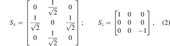
in the usual basis |i⟩ with i = 1, 2, 3. In the whole manuscript, we use the units of vF = ℏ = 1. The above Hamiltonian may be realized in photonic systems [46, 47]. When Vp(x) = 0, for a given momentum k, the free-particle Hamiltonian H0 has three eigenstates and the eigenenergies, i.e.

|−, 0, +; k⟩ denote the states for the lower, middle (flat band) and upper bands, respectively, and E−,k , E0,k , E+,k represent the three corresponding energy bands. It is found that a flat band with zero energy (E0,k = 0) appears between the upper and lower bands (see figure 1). The possible bound states (if any) can only exist in the gaps among the three bands, i.e. 0 < E < m and −m < E < 0 (the regions A and B in figure 1).

Figure 1. (a) The energy spectrum of free-particle Hamiltonian. (b) DOS of the spin-1 Dirac model. The flat band gives rise to an infinitely large DOS at zero energy (thick blue lines). Near the thresholds of upper and lower bands Eth = ±m, the DOS has a similar divergence to that in the ordinary one-dimensional case, i.e.  as E → Eth. Any possible bound states only exist in the regions A and B.
Download figure:
Standard image High-resolution imageIn order to explore the properties of the flat band, we calculate the free-particle Green function G0 (corresponding to H0) and DOS ρ0(x, E) [40]. In momentum space, the free-particle Green function can be expressed as
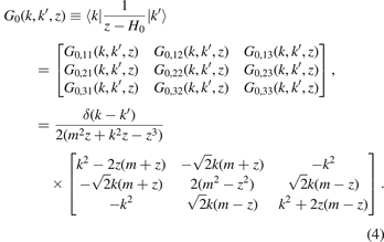
In coordinate space, the matrix elements of the free-particle Green function are [48]

or explicitly written down
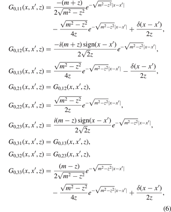
where the sign function sign(x) = 1 for x > 0, sign(x) = −1 for x < 0 and δ(x) is a Dirac delta function. The Dirac delta term δ(x − x')/(2z) in the Green function arises from the flat band, which reflects the localized properties of states in the flat band [32].
The DOS at energy E (per unit length) is given by the imaginary part of the Green function [40], i.e.
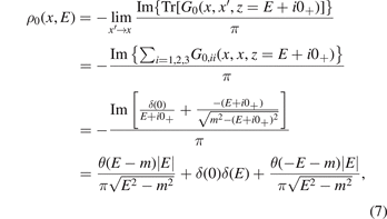
where θ(x) = 1 if x > 0, otherwise θ(x) = 0 and δ(0) = limx'→x δ(x − x') → ∞.
It shows that the flat band of zero energy gives rise to an infinitely large DOS [δ(0)] [42], which reflects the fact that there are infinite states of the flat band in the continuous model. Furthermore, the δ(E) singularity in DOS ρ0(x, E) causes a 1/z singularity in the Green function (see equation (6) and appendix  as E → Eth (see figure 1).
In the following, we will see that such an infinitely large DOS and 1/z singularity of the Green function have important effects on bound states (see appendix
3. Bound states
In the following manuscript, we assume the potential energy Vp has the following diagonal form in the usual basis |i = 1, 2, 3⟩, namely,

3.1. Delta potential
First of all, we assume the potential energy has the form of the delta potential and satisfies V11(x) = V33(x) ≡ 0, and V22(x) = gδ(x) with potential strength g. The Schrödinger equation (Hψ = Eψ) can be written in terms of a three-component wave function, i.e.
Furthermore, using equation (9) to eliminate wave functions for the first and third components, we get an effective Schrödinger equation (second-order differential equation) for ψ2(x):

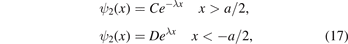
For bound states and x ≠ 0, the wave function ψ2(x) can be written as

where  , C and D are two coefficients for the decayed part of the wave function. The continuity of ψ2(x) at origin x = 0 requires C = D. Integrating both sides of equation (10) near the origin x = 0, it is shown that the derivative of ψ2(x) satisfies

Based on equation (12), the bound-state energy EB is obtained:

First of all, there always exists one bound state whether the potential is repulsive (g > 0) or attractive (g < 0) (see figure 2). However, for the ordinary one-dimensional case, only when the potential is attractive (g < 0), there is one bound state. Secondly, when the potential strength g goes to zero, the bound-state energy EB is linearly proportional to the strength, i.e. EB ∝ g as g → 0 [see panel (b) of figure 2]. Such behavior is very different from the ordinary one-dimensional bound-state energy, which is proportional to g2. The linear dependence on the strength is also consistent with the fact that the superfluid/superconductor order parameter is linearly proportional to the two-body interaction strength in a flat band superfluid system [29, 35, 36]. Most of all these peculiar behaviors are due to the infinitely large DOS of the flat band (see appendix
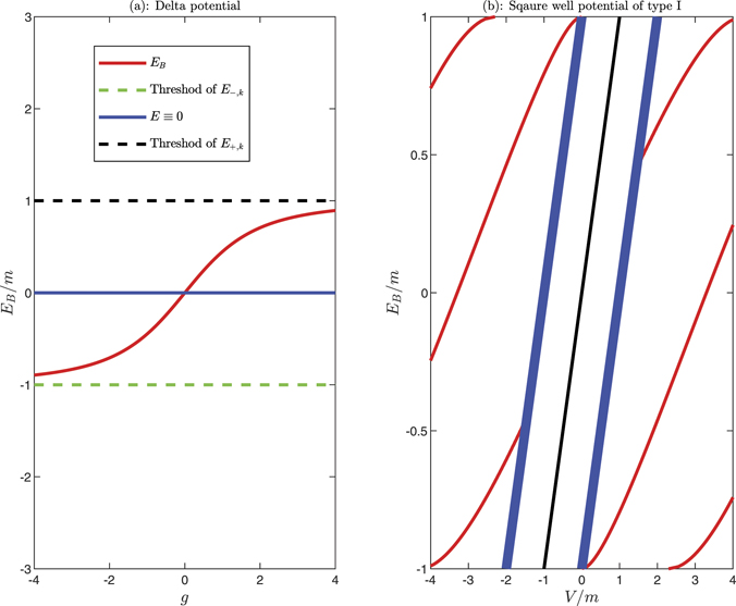
Figure 2. The bound-state energies (the red solid lines). Panel (a) is the bound-state energy of delta potential. Panel (b) is the bound-state energy of square well potential of type I (the red solid lines). Near the thresholds of upper and lower continuums Eth = ±m (|E − m|/m ≪ 1), the bound-state energy can be approximated by equation (22). The (non-trivial) bound states only appear in the regions defined by (E − V)2 − m2 > 0 [see equation (18)]. The two thick blue solid lines are the boundaries of these regions [(E − V)2 − m2 = 0]. The black dashed solid line corresponds to the trivial bound states, which are basically the original states of the flat band with a shifted energy V (see the main text). In panel (b), we take the width of potential well a = 1/m.
Download figure:
Standard image High-resolution imageThirdly, due to the restrictions of the thresholds of the upper and lower continuums, when the potential strength is very large (g → ∞), the bound-state energy EB approaches the thresholds of continuums ±m asymptotically. This is also very different from the usual one-dimensional bound-state energy, which goes to infinity (∝g2 → ∞).
3.2. Square well potential of type I
In this subsection, we assume the potential satisfies V11(x) = V22(x) = V33(x) and
where a > 0 and V are the width and depth (or height) of square well potential, respectively. Now the Schrödinger equation is
Similarly to the above subsection, we get an effective second-order differential equation

In the above derivations, we assume that E − V(x) ≠ 0. For bound states and |x| > a/2 (V11(x) ≡ 0), the wave function ψ2(x) is exponentially decayed, i.e.
where  . For |x| < a/2, the wave function ψ2(x) can be

where 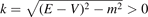 , A and B are two coefficients for the oscillation parts of the wave function.
In the following, we assume that the wave functions for all three components have finite values (they are not infinitely large). Integrating both sides of equation (15) near x = ±a/2, we find ψ2(x) and ψ1(x) + ψ3(x) are continuous functions at x = ±a/2 [21, 45]. Furthermore, taking the relations of
into account, we get equations for coefficients A, B, C and D, i.e.
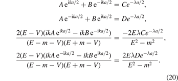
Letting the corresponding determinant vanish, we get an equation for the bound-state energy:
Panel (b) of figure 2 reports the bound-state energy EB as a function of potential strength V. In all the figures, we set the width of the potential well a = 1/m.
When |E − m| ≪ m, and |V| ≪ m, the resulting bound-state energy can be approximated by

It is shown that near the thresholds of continuums ±m, and in the case of weak potential, the bound-state energy (relative to the thresholds) is proportional to the square of strength (EB ± m ∝ V2), which is consistent with the ordinary one-dimensional bound-state energies (see figure 2).
This is because for the square well potential of type I, the three-diagonal matrix elements of potential are equal (in the usual basis |i = 1, 2, 3⟩) [see equation (14)]. One can also view the potential energy in the energy band basis, i.e. |−, k⟩, |0, k⟩ and |+, k⟩; consequently the diagonal form is also not changed approximately. Therefore, for the three energy bands (flat band, upper and lower bands), they have the same potentials V11(x).
For the flat band, the states are spatially localized. Once the potential is turned on, the energy of the states within the range of the potential well only shift by a value of V, i.e. E = 0 → E = V [see the black dashed line in panel (b) of figure 2]. These resulting new states basically inherit the localized properties of the original flat band states. Therefore, we call them trivial bound states (localized flat band states), which we are not interested in.
In addition, near the thresholds of the upper and lower continuums, the DOS has a similar divergence behavior to that in the ordinary one-dimensional case, i.e.  as E → Eth [40] [see figure 1 and equation (7)]. So, in such cases, the bound-state problem can be reduced to an ordinary one-dimensional bound-state problem near the thresholds (especially for shallow bound states). Consequently, the resulting bound-state energies are very similar to the usual one-dimensional results, e.g. EB ± m ∝ V2.
For a given potential strength V, the number of (non-trivial) bound states is always finite for a square well potential of type I (with three equal diagonal matrix elements).
3.3. Square well potential of type II
In this subsection, we assume the potential energy satisfies V11(x) = V33(x) ≡ 0 and
Now the Schrödinger equation can be rewritten as

Similarly to the above subsections, we get an effective Schrodinger equation (second-order differential equation):

In the above derivation, we assume that E ≠ 0.
For bound states and |x| > a/2, the wave function ψ2(x) can be written as

where  . For |x| < a/2, the wave function ψ2(x) is

where }{E}} > 0$](https://content.cld.iop.org/journals/0953-4075/55/6/065001/revision2/bac5582ieqn10.gif) .
.
Similarly, integrating the both sides of equation (24) near x = ±a/2, we find ψ2(x) and ψ1(x) + ψ3(x) are continuous functions at x = ±a/2. Furthermore, taking the relations

into account, it can be shown that the derivative ∂x ψ2(x) at x = ±a/2 is also continuous.
Using these continuity conditions of ψ2(x) at x = ±a/2, we get linear equations for A, B, C and D

In order to have non-trivial solutions to the above linear equations, the corresponding determinant should vanish, i.e.

Then, we get an equation of bound-state energy

where }{E}} > 0$](https://content.cld.iop.org/journals/0953-4075/55/6/065001/revision2/bac5582ieqn11.gif) . Taking a = 1/m, the resulting bound-state energies are reported in figures 3 and 4.
. Taking a = 1/m, the resulting bound-state energies are reported in figures 3 and 4.

Figure 3. The bound-state energy of square well potential of type II. The red solid lines are the exact results of equation (31). When |E/V| ≪ 1, the bound-state energy can be approximated by equation (33) (see the blue dashed lines).
Download figure:
Standard image High-resolution image
Figure 4. The bound-state energy of square well potential of type II. The red solid lines are the exact results of equation (31). When |E/m| ≪ 1, the bound-state energy is given by equation (35) (see the blue dashed lines).
Download figure:
Standard image High-resolution imageWhen |E| ≪ |V|, the above equation (31) is simplified to
So the energy

where the quantum number n = 1, 2, 3, ... (see figure 3). It is shown that there exist infinite bound states, which are generated from the flat band. Due to the infinitely large DOS of the flat band, an arbitrarily small potential V indeed pulls some states out the flat band and then they form bound states. For a given n, when the potential is very strong (V → ±∞), the bound-state energy approaches the thresholds ±m, which is very similar to the delta potential case. For weak potential, the energy is proportional to the potential strength, e.g. En ∝ V.
We should emphasize that the existence of an infinite number of bound states is quite a universal phenomenon in the flat band system with a quite arbitrary potential well of type II (not limited to square well potential; for more explanations see appendix  will be arbitrarily strong, and then the system will have infinite bound states.
Furthermore, when |E| ≪ m, the above equation (32) becomes

so we get the energy

where the quantum number n = 1, 2, 3, ... (see figure 4). It is interesting that the bound-state energy displays a hydrogen atom-like energy spectrum. Outside the square potential well (|x| > a/2), the bound-state wave functions are all exponentially decayed [see equation (26)]. Within the potential well, i.e. |x| < a/2, the wave function oscillates wildly for large quantum n [see equation (27)]. When |E| → 0, the DOS can be approximately obtained:

As |E| → 0, DOS(E) ∝ 1/|E|3/2 → ∞.
The origin of existence of the infinite number of bound states in square well potential is due to the 1/z singularity in the Green function and the δ(E) singularity of the DOS induced by the flat band (see appendices
4. Summary
In conclusion, we analytically calculate the free-particle Green function and DOS for the one-dimensional spin-1 Dirac model. It is found that the infinitely large DOS of the flat band results in a 1/z singularity of the Green function. Furthermore, we solve the bound-state problems in the flat band system for several typical potential wells. It is found that the flat band and its ensuing 1/z singularity of the Green function play crucial roles in the formations of bound states. Due to the 1/z singularity, the bound-state energy shows a linear dependence on the potential strength. In addition, there exists an infinite number of (non-trivial) bound states for some kinds of square well potential. Furthermore, the bound-state energy displays a hydrogen atom-like energy spectrum. Our findings provide alternative ways to get the hydrogen atom-like energy spectrum in condensed matter physics.
Finally, in the presence of long-ranged Coulomb potential, there also exist infinite bound states [55–57]. However, the bound-state energy is usually proportional to 1/n, which is different from 1/n2 of the short-ranged square well potential.
The above findings provide some useful insights and aid our understanding of the many-body physics of the flat band. For example, the infinite bound states induced by small potential imply that an arbitrarily small interaction would dominate the physics, which also reflects the fact that the flat band is not unstable under interactions. Since the bound states can appear for both repulsive (positive strength) and attractive (negative strength) potentials, then one can expect that even a repulsive interaction may result in superfluid/superconductor pairing states in the flat band system [58].
There are also other interesting questions; for example, how to introduce phase shift for the states in the flat band, how the potential affects the phase shifts, what are the relationships between the phase shift and the number of bound states (Levinson theorem) [49–54], etc, need further investigation.
Acknowledgments
YC Zhang thanks Professor Shizhong Zhang for the useful discussions. This work was supported by the NSFC under Grant Nos. 11874127 and 11504095. YC Zhang is also thankful for the startup grant from Guangzhou University.
Data availability statement
All data that support the findings of this study are included within the article (and any supplementary files).
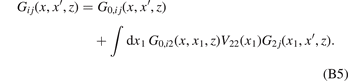
Appendix A.: The relations between the 1/z singularity of Green function and δ (E) singularity of DOS
There exists a general relation between (the trace of) the Green function and DOS [40], i.e.

In addition, if the DOS has a δ(E) singularity, e.g. ρ0(x, E) ∝ δ(E), the Green function behaves as

Furthermore, for a general matrix element of the Green function, if a flat band appears, there also exists the 1/z singularity [see equation (6) in the main text]. It is known that the Green function can be represented as (spectral decomposition)
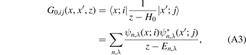
where n is the energy band index, λ denotes other quantum numbers for a given energy band n. Here the eigenfunction ψn,λ
(x) satisfies H0
ψn,λ
(x) = En,λ
ψn,λ
(x). If a flat band appears, for example, En,λ
≡ 0 for some specific index n, G0,ij
(x, x', z) includes a term  , then it would display a 1/z singularity in general. It should be remarked that the above conclusions not only apply to a free-particle Hamiltonian H0, but also to a total Hamiltonian H = H0 + Vp [for example, see equation (1)].
Appendix B.: The importance of 1/z singularity of Green function
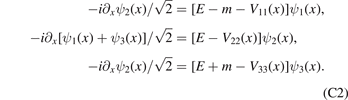
In order to see the importance of 1/z singularity of the Green function in bound-state equations, we reformulate the bound-state problem with the Green function method [40].
First of all, we introduce the full Green function G(z):

which corresponds to the total Hamiltonian H = H0 + Vp. In addition, G(z) satisfies the Lippmann–Shwinger equation, i.e.

where

is the free-particle Green function in operator form. Taking a potential energy in the form of

as an example (both the delta potential and square well potential of type II in section 3 belong to such a class), the Lippmann–Shwinger equation (in coordinate representation) takes the following form:
Specifically, the matrix element
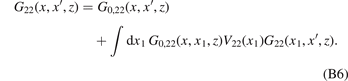
The bound-state solutions are determined by the corresponding homogenous integral equation, namely

For simplification, taking a specific value x' = 0, and setting z = E and G(x) ≡ G22(x, 0, E), the resulting integral equation is

Inserting  [see equation (6) in the main text] in equation (B8), we get
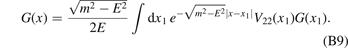
It is shown that the 1/z singularity of the Green function matrix element G0,22 introduces a factor 1/E, which results in the linear dependence on the potential strength in bound-state energy. For example, when the potential is a delta function, i.e. V22(x) = gδ(x), then the integral equation becomes

Then

and

So we can get the bound-state energy

which is consistent with equation (13) in the main text.
In the case of square well potential, the above equation (B9) is essentially equivalent to the effective Schrödinger equation [equation (25) in the main text]. This is because the differential equation equation (25)

can be also transformed into an corresponding integral equation for the bound-state problem. First of all, let us write it in the form of an ordinary second-order Schrödinger equation, e.g.

where the effective total energy  , effective potential energy
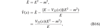
and  for bound states. In the determining effective total energy, we assume the potential energy V22(x) goes to zero as x → ±∞. It shows that when V/E > 0, the effective potential
  is attractive, and then bound states would exist in one dimension. Furthermore, if the energy is very small, e.g. 0 < E/V ≪ 1 and |E|/m ≪ 1, the effective potential strength can be arbitrarily large
  , so there would exist infinite bound states. We see that the factor 1/E plays crucial roles in the existence of an infinite number of bound states.
It should be remarked that the existence of infinite bound states is quite a universal phenomenon in the flat band system with a potential well of type II. This is because as long as the energy E is sufficiently small, the factor 1/E would result in an arbitrarily strong effective potential  . Consequently, a strong effective potential would support infinite bound states.
The integral equation corresponding to the above equation (B15) is

where the effective free-particle Green function (corresponding to the effective Hamiltonian  in one dimension) [40] is

Inserting it in equation (B17), then

It is found that G(x) and ψ2(x) satisfy the same integral equation for bound states [see equations (B9) and (B19)]. During the above derivations, we see that 1/z singularity in the Green function is very important in the bound-state equation. The 1/z singularity has close relations to the factor E in the denominator of the effective potential  [see equations (B16), (B9) and (B19)]. Most of the peculiar behaviors of bound-state energies, for example linear dependence on the potential strength, an infinite number of bound states and a hydrogen atom-like spectrum, can be attributed to the 1/z singularity of the Green function.
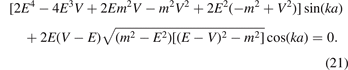
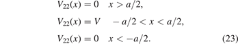
Appendix C.: Square well potential of type III
In this appendix, we discuss the bound states for other types of square well potentials. First of all, we assume all the matrix elements V11(x), V22(x) and V22(x) are square well potentials with same width a, i.e.
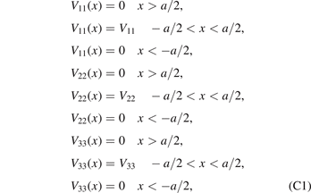
where V11, V22 and V33 are the potential strengths of V11(x), V22(x) and V22(x), respectively.
Now the Schrödinger equation can be rewritten as
Similarly, eliminating ψ1(x) and ψ3(x), we get
When |x| > a/2, the bound-state wave function ψ2(x) can be written as

where  . For |x| < a/2, the wave function ψ2(x) is

where

Integrating both sides of equation (C2) near x = ±a/2, we find ψ2(x) and ψ1(x) + ψ3(x) are continuous functions near x = ±a/2. Furthermore, taking the relations

into account, we get
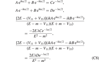
Letting the corresponding determinant vanish, we can get bound-state energies. When V11 = V22 = V33 = V, the bound-state energy is reduced to equation (21) of potential of type I. Meanwhile, when V11 = V33 ≡ 0, V22 = V, the bound-state energy is given by equation (31) of type II. We see for a given potential strength V, there exist finite bound states in the case of type I, while the system has infinite bound states in the case of type II.
From the discussions in appendix B, we know that a crucial requirement for the existence of infinite bound states is that the effective potential [or wave vector k in equation (C6)] can become infinitely large. So if the denominator of k2 [see equation (C6)] cannot be canceled by the numerator, the wave vector k and effective potential can be arbitrarily large for some E. Then, there would exist infinite bound states. However, when the denominator of k2 can be canceled by the its numerator, the wave vector k is always finite. In such a case, the system only has finite bound states, e.g. the case of V11 = V22 = V33 = V (the case of type I).
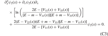
In the following, we investigate the case of V22 = V33 ≡ 0, V11 = V, where the denominator of k2 cannot be canceled by its numerator. Then it is expected that there would exist infinite bound states. In the whole manuscript, we refer to such type of potential as type III. The bound-state energy equation is
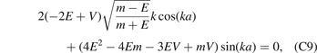
where ![$k=\sqrt{\frac{2E(E+m)[E-m-V]}{2E-V}} > 0$](https://content.cld.iop.org/journals/0953-4075/55/6/065001/revision2/bac5582ieqn24.gif) . The results are reported in figures 5 and 6. When V < 0 and E → Eth = m, the resulting bound-state energy
. The results are reported in figures 5 and 6. When V < 0 and E → Eth = m, the resulting bound-state energy

which is also consistent with result of one-dimensional bound states [see figures 2 and 5 and equation (22)].

Figure 5. The bound-state energy of square well potential of type III. The red solid lines are the exact results of equation (C9). When V < 0 and |E/m| ≪ 1, the bound-state energy can be approximated by the equation (C10). Near the black line (E = V/2), there also exist infinite bound states.
Download figure:
Standard image High-resolution image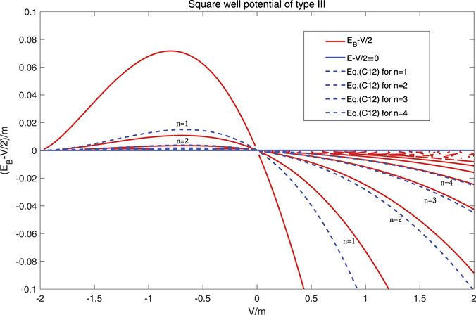
Figure 6. The bound-state energy (relative to V/2) of square well potential of type III. The red solid lines are the exact results of equation (C9). Furthermore, when |E − V/2|/m ≪ 1, the bound-state energy is approximated by equation (C12) (see the blue dashed lines).
Download figure:
Standard image High-resolution image
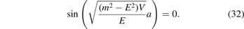
In addition, when the energy E approaches V/2, e.g. 2E − V → 0, the wave vector k → ∞. Consequently, there exist infinite bound states near the line E = V/2 (see black line of figure 5). When |E − V/2|/m ≪ 1, the above equation (C9) is simplified into

Then we get the energy

where n = 1, 2, 3, ... There also exist infinite bound states for arbitrarily small potential strength V (see figure 5). The bound-state energy (relative to V/2) also displays the hydrogen atom-like energy spectrum (see figure 6).
The above discussions indicate that, for other types of square well potentials and general potential strengths, there also exist infinite bound states and a 1/n2 energy spectrum.