


Introduction
A key element to improve the functionality of novel materials is the ability to observe and characterize the dynamic events of nanoscale systems (e.g., atomic migration and fluxional behavior). The ultimate goal is to fully describe and understand the mechanisms where atomic rearrangements occur with high time resolution at the atomic scale. While ultra-fast transmission electron microscopy (TEM) can provide time resolutions at nanoseconds or shorter, they cannot deliver atomic resolution information (LaGrange et al., Reference LaGrange, Reed, Santala, McKeown, Kulovits, Wiezorek, Nikolova, Rosei, Siwick and Campbell2012). When time resolutions on the order of milliseconds are desired, in situ TEM, equipped with direct electron detection systems, is a suitable technique. This approach can provide information such as dynamic strain and cation diffusion, as recently demonstrated for nanoparticles surface sites (Lawrence et al., Reference Lawrence, Levin, Miller and Crozier2019, Reference Lawrence, Levin, Boland, Chang and Crozier2021). The relevance of such fluxional behavior to catalysis has recently been recognized (Guo et al., Reference Guo, Sautet and Alexandrova2020; Sun et al., Reference Sun, Alexandrova and Sautet2020; Vincent & Crozier, Reference Vincent and Crozier2021), and is described as active structures constantly transitioning through metastable states far from equilibrium. Non-equilibrium, evolving metastable structures may play a crucial role in electrochemistry for next-generation batteries (Mehdi et al., Reference Mehdi, Qian, Nasybulin, Park, Welch, Faller, Mehta, Henderson, Xu, Wang, Evans, Liu, Zhang, Mueller and Browning2015; Ma et al., Reference Ma, Cheng, Yin, Luo, Sharafi, Sakamoto, Li, More, Dudney and Chi2016), phase transformations (Heo et al., Reference Heo, Dumett Torres, Banerjee and Jain2019; Moehring et al., Reference Moehring, Fort, McBride, Kato, Macdonald and Kidambi2020), or chemical reactions where gas–solid and liquid–solid interactions occur during catalysis (Tao & Crozier, Reference Tao and Crozier2016; Yuan et al., Reference Yuan, Wang, Li, Wu, Zhang, Selloni and Sun2016, Reference Yuan, Zhu, Li, Hansen, Ou, Fang, Yang, Zhang, Wagner, Gao and Wang2020; Zhang et al., Reference Zhang, Plessow, Willis, Dai, Xu, Graham, Cargnello, Abild-Pedersen and Pan2016; Li et al., Reference Li, Kottwitz, Vincent, Enright, Liu, Zhang, Huang, Senanayake, Yang, Crozier, Nuzzo and Frenkel2021).
To understand such phenomena, it is necessary to have both high spatial and temporal resolutions in order to determine the atomic-level dynamics (Furnival et al., Reference Furnival, Knez, Schmidt, Leary, Kothleitner, Hofer, Bristowe and Midgley2018, Lawrence et al., Reference Lawrence, Levin, Miller and Crozier2019). Z-contrast STEM is an excellent approach for performing atomic-level discrete tomography of nanoparticle structures because the linear relationship between the number of atoms in the column and the image intensity extends over a wider range of thickness (Gonnissen et al., Reference Gonnissen, De Backer, den Dekker, Sijbers and Van Aert2017). However, at present, the temporal resolution of STEM imaging is limited because of the serial nature of the image formation process. For high time resolution, phase contrast TEM is faster since it performs parallel pixel readout. For example, the experimental data presented here was extracted from 4 k × 4 k TEM image sequence recorded at 400 frames per second. To acquire such data using STEM would require dwell times approaching a nanosecond that are not currently available. In phase contrast TEM, the relationship between the image intensity and the atomic column number is more complex but can be managed through image simulation at least for small nanoparticles and surfaces structures of interest here.
Recent developments on direct electron detectors allow image acquisition at up to 1,000 frames per second with a higher detective quantum efficiency, reducing additional sources of noise (e.g., readout noise, photon conversion noise, etc.) (McMullan et al., Reference McMullan, Faruqi, Clare and Henderson2014; Faruqi & McMullan, Reference Faruqi and McMullan2018; Ciston et al., Reference Ciston, Johnson, Draney, Ercius, Fong, Goldschmidt, Joseph, Lee, Mueller, Ophus, Selvarajan, Skinner, Stezelberger, Tindall, Minor and Denes2019) making them ideal to track evolving structures or image radiation-sensitive materials (Chen et al., Reference Chen, Dwyer, Sheng, Zhu, Li, Zheng and Zhu2020). However, the individual images associated with higher temporal resolution show a poor signal-to-noise ratio (SNR) due to the lower number of electrons arriving at the detector within the short exposure time. The presence of a high noise reduces the precision in determining the position and intensity of atomic columns, and this has motivated the development of denoising techniques (Du, Reference Du2015; Furnival et al., Reference Furnival, Leary and Midgley2017; Vincent et al., Reference Vincent, Manzorro, Mohan, Tang, Sheth, Simoncelli, Matesson, Fernandez-Granda and Crozier2021). However, these denoising methods may not always perform well so it is important to develop complementary noise-robust procedures to determine columns positions and intensities in the presence of high noise.
The electron microscopy community already offers multiple state-of-the-art algorithms addressing the position and intensity of atomic columns, and most of them fit a two-dimensional Gaussian to the atomic columns in the images (Yankovich et al., Reference Yankovich, Berkels, Dahmen, Binev, Sanchez, Bradley, Li, Szlufarska and Voyles2014; Mukherjee et al., Reference Mukherjee, Miao, Stone and Alem2020). For example, Atomap (Nord et al., Reference Nord, Vullum, MacLaren, Tybell and Holmestad2017) is a well-known Python-based code tailored for STEM images, where in the particular case of HAADF-STEM images (Z-contrast imaging), the intensity of the atoms is bright and is linearly proportional to the thickness. On the other hand, TRACT (Levin et al., Reference Levin, Lawrence and Crozier2020) is a MATLAB algorithm developed mainly for bright-field HRTEM images, whose background signal could be either higher or lower than the atomic columns (black or white intensity, depending on the imaging conditions). However, these methods have been traditionally applied to images with reasonable SNRs, and there is a lack of information about the performance of these 2D Gaussian fitting algorithms on images with poor SNR. More sophisticated procedures are based on machine learning and neural networks, as proposed on TEMImageNet (Lin et al., Reference Lin, Zhang, Wang, Yang and Xin2021), but require large simulated dataset and extensive training of the network.
Here, we develop and test a method to determine the atomic column position and intensity based on a hybrid approach that combines Gaussian peak fitting with a blob detection scheme (Lindeberg, Reference Lindeberg1993), which has been previously established in the computer vision community. We show that the hybrid blob detection approach significantly outperforms approaches based solely on Gaussian peak fitting for noisy data.
Materials and Methods
Introduction to Blob Detection (BD) Algorithm
We have employed blob detection (BD) algorithms (Lindeberg, Reference Lindeberg1993), specifically, those available in the Python package skimage (van der Walt et al., Reference van der Walt, Schönberger, Nunez-Iglesias, Boulogne, Warner, Yager, Gouillart and Yu2014). We find that standard BD works to locate the rough positions of atomic columns, but to further improve precision we introduce additional steps, illustrated in Figure 1, to refine the position and column intensity estimation. Indeed, blob detection routines, which are popular and well-developed methods in the field of computer vision (Lowe, Reference Lowe2004; Kong et al., Reference Kong, Akakin and Sarma2013; Xu et al., Reference Xu, Wu, Gao, Charlton and Bennett2020), are generally used to find regions within images that differ in certain properties, for example, in brightness, relative to neighboring regions. There are different forms of BD methods, and herein we will refer to two specific methods that outperform in both simulations and experiments: the “Laplacian of Gaussian” (LoG) method (Lindeberg, Reference Lindeberg1993, Reference Lindeberg1998) and the “Difference of Gaussian” (DoG) method (Lindeberg, Reference Lindeberg2015). A general sketch illustrating the workflow of BD algorithm is shown in Supplementary Figure S1.

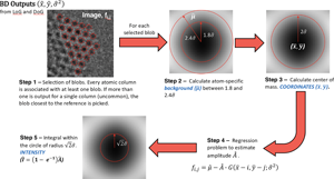
Fig. 1. General scheme on how the coordinates and the intensity  $\hat{I}$ of atomic columns are calculated starting from the blob detection algorithm output. The five steps followed on the procedure are further explain with details in the methodological section “Tailored adjustments for our specific experimental dataset”. Images on Steps 2, 3, and 5 show a simulated atomic column in TEM mode.
Before proceeding to the algorithm, we first introduce some notation and highlight relevant background information. The size of the images we consider is denoted as m × n, and the pixel lattice coordinates are given by the set Ω = {(i, j): i = 1, …, m, j = 1, …, n}. We introduce the mapping f(x, y) such that the pixel values of a TEM image are denoted as f i,j = f(x = i, y = j) > 0 for pixel indices (i, j) ∈ Ω. Note that in TEM images, areas with no sample are considered as measurements of the vacuum background, for example, the top-right corner of Figure 2 is unstructured noise; we denote f B to be the average pixel values in the vacuum background. In addition, we denote  $f^\alpha$ to be α = 5th-percentile from all the pixel values{f i,j:(i, j) ∈ Ω}. We define a two-dimensional, mean zero, spherical Gaussian density function as:
 $$G( {x, \;y, \;\sigma^2} ) = \Phi ( {( {x, \;y} ) , \;( {\mu_X, \;\mu_Y} ) = ( {0, \;0} ) , \;{\rm \Sigma } = \sigma^2I_2} ) = {\rm \;}\displaystyle{1 \over {2\pi {\rm \sigma }^2}}\exp \left({-\displaystyle{{x^2 + y^2} \over {2{\rm \sigma }^2}}} \right)$$
Fig. 2. Fluxional behavior in time-resolved in situ TEM experimental data. Images have been contrast-reversed following equation (2). (a) 2.5 s summed image of a CeO2 nanoparticle, presenting a good signal-to-noise ratio which enables to efficiently resolve the position and the intensity of each present atomic column. (b) and (c) illustrate a 37.5 ms summed image at two different periods of time, where the red arrows indicate the disappearance of two atomic columns, this indicating that the summed image (a) is not representative for all the frames in the time series. (d) Time-resolved single frame of the experimental data, 2.5 ms, pointing out that the high content of noise (SNR = ~4) hinders the determination of the time the evolution of each atomic column. (e1) and (e2) represent a surface and bulk column, respectively, showing the difficulty of determining the central position and intensity of the atomic columns, especially on those at the surface where more dynamics are taking place.
for example, with mean (μ X, μ Y) = (0, 0) and the single-scale parameter σ 2, where Φ denotes the standard bivariate Gaussian density function. We now introduce our full BD algorithm through the definitions and steps below, highlighting our additional tailoring to this specific problem.
Conventionally, the BD function of the Python's skimage package seeks bright pixels surrounded by darker ones (e.g., Supplementary Fig. S1a). However, the particular bright-field experimental data presented in this work was recorded initially with a bright background and black contrast of atomic columns, such that the regions of interest (the atomic columns) are darker than their surroundings. Hence, we introduce the following preprocessing step for experimental TEM images.
Definition 0. Define the function F(x, y) that generates a contrast reversal of the original image values f at (i, j) ∈ Ω as:
 $$F_{i, j} = F( {X = i, \;Y = j} ) = {\rm \;}\displaystyle{{\,f^B-f_{i, j}} \over {\,f^B-f^\alpha }}, \;$$
resulting in bright atomic columns (high pixel values) surrounded by dark background.
Remark on Definition 0. In equation (2), the numerator is reversing the contrast, while the denominator,  $f^B-f^\alpha$, is used to normalize the observations. Additional subtraction by
  $f^\alpha$ in the denominator is performed such that the majority of the mapped values {F i,j:(i, j) ∈ Ω} will be less than one, especially at the locations {(i, j)} of primary interest within the black contrast of an atomic column (where f i,j ≤ f B usually holds). Such preprocessed values F i,j will also tend to be distributed within [0, 1] quite densely, that is, 0 ≤ F i,j ≤ 1 regardless of the raw observations f i,j. As an added benefit, the BD parameters, as estimated below, under this normalized transformation may also be applied with similar detection power on new images with comparable SNRs, but independent of the new image's specific scaling. In practice, we have used the 5th-percentile for
  $f^\alpha$, as noted above; however, other percentiles in the range 1–10 may also be used depending on how variable or stable low percentile signal values behave.
Definition 1. The BD algorithm begins by convolving (discretely and finitely) the contrast reversed image {F i,j:(i, j) ∈ Ω} with the Gaussian function G(x, y, σ 2) at the pixel locations Ω, illustrated in Supplementary Figure S1. Specifically, we define the convolution function C(x, y, σ 2) as:
 $$C( {x, \;y, \;\sigma^2} ) = G( {x, \;y, \;\sigma^2} ) {\rm \ast }F( {x, \;y} ) = \mathop \sum \limits_{( {i, j} ) \in {\rm \Omega }} G( {x-i, \;y-j, \;\sigma^2} ) \cdot F_{i, j}.$$
With this definition for the convolution function C(x, y, σ 2), we next introduce the two objective functions that are optimized within the LoG and DoG methods, respectively.
Remark on Definition 1. In addition to smoothing out the features arising from noise, the discrete Gaussian convolution is used to match our model Assumption 1 given later, and help determine the Gaussian parameters (both coordinates and variance) of the atomic columns (Supplementary Fig. S1).
Definition 2. We define L(x, y, σ 2) as the (scale-normalized) Laplacian, or second derivative of function C(x, y, σ 2), as:
 $$L( {x, \;y, \;\sigma^2} ) = {\rm \;}\sigma ^2\Delta C( {x, \;y, \;\sigma^2} ) = {\rm \;}\sigma ^2\mathop \sum \limits_{( {i, j} ) \in {\rm \Omega }} {\rm \Delta }G( {x-i, \;y-j, \;\sigma^2} ) \cdot F_{i, j}, \;$$
in which ΔC(x, y, σ 2) = C xx(x, y, σ 2) + C yy(x, y, σ 2) and ΔG(x, y, σ 2) = G xx(x, y, σ 2) + G yy(x, y, σ 2) denote the Laplacian operators of the function C(x, y, σ 2) in equation (3) and G(x, y, σ 2) in equation (1) with respect to x and y, respectively.
We further define Q(x, y, σ 2) as the (scale-normalized) first derivative of C(x, y, σ 2) with respect to σ 2:
 $$Q( {x, \;y, \;\sigma^2} ) = \sigma ^2C_{\sigma ^2}( {x, \;y, \;\sigma^2} ).$$
Remark on Definition 2. The scale parameter σ 2 is included in both functions L(x, y, σ 2) and Q(x, y, σ 2) so that in addition to estimating the center locations of blobs, the minimization of the objective functions can also automatically match the exact scale/shape of the underlying blobs (see Lindeberg, Reference Lindeberg1998).
In practice, the BD algorithm evaluates the functions L(x, y, σ 2) or Q(x, y, σ 2) discretely at (x, y) = (i, j) ∈ Ω and  $\sigma ^2 = \sigma _k^2 \in {\rm \Psi } = { {\sigma_1^2 , \;\cdots , \;\sigma_K^2 } }$, where
  $\sigma _1^2 \le \cdots \le \sigma _K^2$ are user-specified equally spaced BD variance parameters for discrete and approximate optimization. The Python function takes σ 1, σ K, and K as the input and automatically generates the corresponding arithmetical sequence Ψ. These sets generate a three-dimensional array of evaluation points for the final objective function. In the literature (Lindeberg, Reference Lindeberg2015), the partial derivatives appearing in equation (5) is usually approximated using discrete finite difference. Specifically, denoting Λ = Ω × {1, …, K} and
  $C[ {i, \;j, \;k} ] = C( {x = i, \;y = j, \;\sigma^2 = \sigma_k^2 } )$, for (i, j, k) ∈ Λ, we have
 $$C_{\sigma ^2}( {x = i, \;y = j, \;\sigma^2 = \sigma_k^2 } ) \approx \tilde{C}_{\sigma ^2}[ {i, \;j, \;k} ] \triangleq ( {C[ {i, \;j, \;k + 1} ] {-C} [{i, \;j, \;k} ] } ) /( {\sigma_{k + 1}^2 -\sigma_k^2 } ).$$
Hence, for (i, j, k) ∈ Λ, we have
 $$L( {x = i, \;y = j, \;\sigma^2 = \sigma_k^2 } ) = \tilde{L}[ {i, \;j, \;k} ] $$
which can be directly evaluated according to equation (4), and
 $$Q( {x = i, \;y = j, \;\sigma^2 = \sigma_k^2 } ) = \tilde{Q}[ {i, \;j, \;k} ] \triangleq \sigma _k^2 \tilde{C}_{\sigma ^2}[ {i, \;j, \;k} ].$$
 The LoG method of the BD algorithm approximately minimizes the objective function L(x, y, σ 2) by searching for the local minimums across the 3D array  $\tilde{L} = { {\tilde{L}[ {i, \;j, \;k} ] \colon ( {i, \;j, \;k} ) \in {\rm \Lambda }} }$, that is, those points that have values below a given threshold (δ) as compared with their immediate (3 × 3 × 3) neighbors in this array (see Supplementary Fig. S1e). The DoG branch does the same (local) minimization search, except for the array
  $\tilde{Q} = { {\tilde{Q}[ {i, \;j, \;k} ] \colon ( {i, \;j, \;k} ) \in {\rm \Lambda }} }$ instead.
Definition 3. The local minimum indices  ${ {( {{\hat{x}}_r, \;{\hat{y}}_r, \;{\hat{k}}_r} ) \in {\rm \Lambda }\colon r = 1, \;\ldots , \;R} }$ of the 3D array
  $\tilde{L}$ given a threshold δ satisfy:
 $$ \eqalignb{& \tilde{L}[ {{\hat{x}}_r, \;{\hat{y}}_r, \;{\hat{k}}_r} ] < \tilde{L}[ {i, \;j, \;k} ] - \delta , \; \cr & {\rm \;for\;} \left\{{\matrix{ {i = {\hat{x}}_r-1, \;{\hat{x}}_r, \;{\hat{x}}_r + 1, \;} \cr {\,j = {\hat{y}}_r-1, \;{\hat{y}}_r, \;{\hat{y}}_r + 1, \;} \cr {k = {\hat{k}}_r-1, \;{\hat{k}}_r, \;{\hat{k}}_r + 1, \;} \cr } } \right.{\rm \;and\;}( {i, \;j, \;k} ) \ne ( {{\hat{x}}_r, \;{\hat{y}}_r, \;{\hat{k}}_r} ).$$
And an image's candidate blob set is hence defined as:
 $$B_\delta ^{\rm LoG} = { {b_r = ( {{\hat{x}}_r, \;{\hat{y}}_r, \;\sigma_{{\hat{k}}_r}^2 } ) \in {\rm \Omega } \times {\rm \Psi }\colon r = 1, \;\ldots , \;R} }.$$
 Remark on Definition 3. The blob set  $B_\delta ^{\rm DoG}$ from the other array
  $\tilde{Q}$ can be analogously defined given a threshold δ. With no further notice, the blob-like triplet b = (x, y, σ 2) will always be regarded as the circle centered at (x, y) with radius 2σ, including its edge. Instead of using radius
  $\sqrt 2 \sigma _{{\hat{k}}_r}$ as in the generic case described by skimage package (Lindeberg, Reference Lindeberg1993), we use the expanded radius
  $2\sigma _{{\hat{k}}_r}$ in order to have a larger blob area to compute the center of mass (as detailed below). Rather than outputting all local minimums, the function in the Python package preprocesses and removes largely overlapping blobs. To be specific, if the overlapping area of two of these blobs exceeds a given percentage (γ), then the smaller circle is eliminated from the set of blobs. Additionally, the generic version of BD only allows concentrically symmetric blobs, otherwise irregularly shaped atomic columns may be associated with multiple connected blobs. Ideally speaking, if the input image {f i,j:(i, j) ∈ Ω} is well-conditioned, that is, with high SNR and well-separated nanoparticle structures, the number of detected blobs R should be equal (or close) to the number of atomic columns.
To summarize, for the optimal performance of a BD algorithm, the parameters that require careful initializations include the prefixed BD variance parameters Ψ (minimum and maximum sigma, and the number of steps between them), the threshold for local minimums δ, and the overlapping blob percentage γ (value between 0 and 1). As an example, Table 1 shows the parameters we have used for our simulated and experimental datasets. We have implemented LoG and DoG to our dataset and it turned out that both methods return excellent initial blobs for our following steps. Notice that the blobs are determined to within one pixel accuracy, sub-pixel refinement is performed at a later stage [see discussion of equation (14) below].
Table 1. Initialization Parameters Used in Our Noise-Free, Noisy, and Experimental Datasets.

Atomic Information Extraction and Refinements
Based on the general BD approach detailed above, we further introduce our tailored proposal for atom identification in time-resolved TEM image series. In particular, we utilize the output from a BD algorithm as our initial information regarding the atomic columns, we compute the blob area-based center of mass to refine estimates of column positions, and fit a weighted linear regression model to estimate the blob-based column intensities using our modeling assumptions detailed below. These steps, that are described in detail in the following paragraphs, are shown in Figure 1.
To eliminate the influence between different atomic columns due to the convolution equation (3) across the whole images, and to avoid the challenge of labeling detected blobs from the BD function with atomic columns’ indices, we choose not to implement BD globally on the whole image field of view. Instead, we implement separately within user-specified sub-region that roughly correspond to the approximate position of specific atomic columns (one sub-region per atomic column). Indeed, such idea also saves the computational power since the sizes of the arrays  $\tilde{L}$ and
  $\tilde{Q}$ decrease significantly. Typically, a time series of image frames is considered for analysis. First, by summing all or a subset of the frames pixel-wise across the time series, the size and location of each search region can be chosen to guarantee that the sub-image is large enough to contain an atomic column, while sufficiently small to ensure that neighboring columns are not included. Then, the following tailored steps are applied sequentially to all atomic columns to recover the underlying nanoparticle structure within an image. Hence from now we will update the notation Ω as the indices set of the sub-images.
To begin, we first propose the following assumption, similar to Levin et al. (Reference Levin, Lawrence and Crozier2020), to model the pixel behavior of a specific atomic column.
Assumption 1. The pixel values within the atomic column can be exactly parametrized by the blob-like triplet  $b_0 = ( {x_0, \;{\rm \;}y_0, \;{\rm \;}\sigma_0^2 } )$. In addition, every pixel (i, j) ∈ Ω within or near (as defined below) the circle b 0 satisfies:
 $$f_{i, j} = \mu -A\cdot G( {x = x_0-i, \;y = y_0-j, \;\sigma^2 = \sigma_0^2 } ) , \;$$
where A is a scale for the Gaussian function, which is varying relative to the number of atoms present, and μ is the background intensity level (both defined below); and G(x, y, σ 2) is the Gaussian density function as defined in equation (1). Equivalently, the contrast behavior for the atomic column compared to its neighborhood can be derived directly from equation (11) as:
 $$A\cdot G( {x = x_0-i, \;y = y_0-j; \;\sigma^2 = \sigma_0^2 } ) = \mu -f_{i, j}.$$
 Remark on Assumption 1. The parameters A and μ appearing in equations (11) and (12) are unknown and to be estimated as  $\hat{A}$ and
  $\hat{\mu }$ in the steps below. Note that in TEM imaging, the background level μ is atomic-column specific since the intensity values in the surrounding region of the atomic column depend on the number of atoms present, and it differs from the value in the vacuum (Gonnissen et al., Reference Gonnissen, De Backer, den Dekker, Sijbers and Van Aert2017), that is, μ will differ from f B, in general.
Further note that in the following discussion, we derive our procedure with respect to {f i,j:(i, j) ∈ Ω} not the contrast reversed {F i,j:(i, j) ∈ Ω} to make later more straightforward comparisons with competing methods for column intensity estimation.
Recall in Definition 3 for the general introduction of BD approach, we define equation (10) as the set of candidate blobs from the LoG method (DoG analogously). For simplicity, in the following definition, Λ now represents the collection of sub-image pixels, and we continue using the same notation of equation (10) but for the BD output targeted at a specific atomic column region within an image.
Definition 4. Given the extracted sub-image's size, calibrated by the summed image sequence, the output of BD for a specific atomic column region is:
 $$B = { {b_1 = ( {{\hat{x}}_1, \;{\hat{y}}_1, \;\sigma_{{\hat{k}}_1}^2 } ) , \;\cdots , \;b_R = ( {{\hat{x}}_R, \;{\hat{y}}_R, \;\sigma_{{\hat{k}}_R}^2 } ) } } \subset {\rm \Lambda }.$$
Remark of Definition 4. In practice, we can implement both LoG and DoG methods, and combine the returned blobs together to obtain the set B as given in equation (13) after removing repeated and overlapping blobs. Unlike BD applied to the entire image, the number of blobs in the output set B for a single atomic column region is generally one (R = 1), however, in the current experimental dataset, there are some very noisy frames in which we find two (or even more) blobs within the image sub-region. When more than one blob is returned for a particular atomic column, reference coordinates are required to help pinpoint the optimal blob. With the summed image sequence mentioned above, which has a relatively high SNR, the average position of the atomic column can more easily be estimated, however, it then lacks all dynamics taking place across the sequence of images.
Definition 5. Define reference coordinates of an atomic column as b* = (x*, y*), that is, those from a summed sequence of images.
Whenever the set B has multiple blobs, the following proposition details how to proceed and denotes the final notation for the unique blob mapped to that atomic column.
Step 1. The blob b r in candidate set B whose center  $( {{\hat{x}}_r, \;{\hat{y}}_r} )$ has the shortest Euclidean distance to reference b* is selected to represent the specific atomic column when there is more than one returned. Denote the selected blob as
  $\hat{b} = ( {\hat{x}, \;\hat{y}, \;{\hat{\sigma }}^2} )$.
Remark on Step 1. In expectation, among our search grid Λ, the selected output  $\hat{b} = ( {\hat{x}, \;\hat{y}, \;{\hat{\sigma }}^2} )$ will be the closest discrete location to the ground truth
  $b_0 = ( {x_0, \;{\rm \;}y_0, \;\;\sigma_0^2 } )$ defined in Assumption 1.
With the final blob estimate  $\hat{b} = ( {\hat{x}, \;\hat{y}, \;{\hat{\sigma }}^2} )$ given, we now detail our tailoring for recovering the coefficients A and μ in model Assumption 1 (equation (12)), followed by our approach for more precisely estimating an (integrated) intensity for that atomic column.
We estimate the atom-specific background level μ to be the average of the pixel values near the edge of the blob circle  $\hat{b} = ( {\hat{x}, \;\hat{y}, \;{\hat{\sigma }}^2} )$ which approximates
  $b_0 = ( {x_0, \;y_0, \;{\rm \;}\sigma_0^2 } )$.
Step 2. The atom-specific background estimator  $\hat{\mu }$ for μ is computed as the average pixel values inside the annulus region with center
  $( {\hat{x}, \;\hat{y}} )$ and radii
  $1.8\hat{\sigma }$ and
  $2.4\hat{\sigma }$, respectively.
Given the lack of inherent precision for the discrete location coordinates  $( {\hat{x}, \;\hat{y}} ) \in {\rm \Omega }$, we propose a center of mass analysis that converts integer-valued coordinates
  $( {\hat{x}, \;\hat{y}} ) \in {\rm \Omega }$ to the real-valued pair
  $( {\bar{x}, \;\bar{y}} )$, which provides sub-pixel level precision.
Step 3. Given the estimated background level  $\hat{\mu }$, the center of mass is then computed within the circle defined by
  $\hat{b} = ( {\hat{x}, \;\hat{y}, \;{\hat{\sigma }}^2} )$ as
 $$\bar{x} = \displaystyle{{\sum\nolimits_{( {i, j} ) \in \hat{b}} {i\cdot {( {\hat{\mu }-f_{i, j}} ) }_ + } } \over {\sum\nolimits_{( {i, j} ) \in \hat{b}} {{( {\hat{\mu }-f_{i, j}} ) }_ + } }}, \;{\rm \;}\bar{y} = \displaystyle{{\sum\nolimits_{( {i, j} ) \in \hat{b}} {\,j\cdot {( {\hat{\mu }-f_{i, j}} ) }_ + } } \over {\sum\nolimits_{( {i, j} ) \in \hat{b}} {{( {\hat{\mu }-f_{i, j}} ) }_ + } }}, \;$$
where  $( {\hat{\mu }-f_{i, j}} ) _ + { = } {\rm max}( {0, \;{\rm \;}\hat{\mu }-f_{i, j}} )$ is the non-negative weight for pixel
  $( {i, \;j} ) \in \hat{b}$.
Note that in equation (12), the scaling or amplitude A is now the only parameter that remains un-estimated if we further assume that  $b_0\approx \bar{b} = ( {\bar{x}, \;\bar{y}, \;{\hat{\sigma }}^2} )$ and
  $G( {x = x_0-i, \;y = y_0-j; $
  $\sigma^2 = \sigma_0^2 } ) \approx G( {x = \bar{x}-i, \;y = \bar{y}-j; \;\sigma^2 = {\hat{\sigma }}^2} )$ for all pixel coordinates (i, j) in or around circle
  $\bar{b}$. In fact, the same equation (12) holds for every pixel (i, j) within the blob
  $\bar{b}$ except the parameters
  $( {x_0, \;y_0, \;\sigma_0^2 } )$ replaced by
  $( {\bar{x}, \;\bar{y}, \;{\hat{\sigma }}^2} )$; hence, a weighted least square regression is proposed to estimate the amplitude A.
Step 4. The amplitude A can be estimated by the following regression problem:
 $$\hat{A} = \mathop {{\rm argmin}}\limits_{a > 0} \mathop \sum \limits_{( {i, j} ) \in \bar{b}} \bar{G}[ {i, \;j} ] \cdot ( {\hat{\mu }-f_{i, j}-a\cdot \bar{G}[ {i, \;j} ] } ) ^2, \;$$
where  $\bar{G}[ {i, \;j} ] = G( {x = \bar{x}-i, \;y = \bar{y}-j; \;\sigma^2 = {\hat{\sigma }}^2} )$, and G is the Gaussian function defined in equation (1).
Our final step is to compute an integrated intensity estimate for the atomic column, and this can be done analytically via integration, based on the estimated model parameters derived above. For better comparisons with alternative methods for estimating the integrated intensity for an atomic column, we narrow the integration region to be  $\tilde{b} = ( {\bar{x}, \;\bar{y}, \;( {\hat{\sigma }}^2/2) } )$, that is, the circle with center
  $( {\bar{x}, \;\bar{y}} )$ and radius
  $\sqrt 2 \hat{\sigma }$.
Step 5. With  $\bar{b} = ( {\bar{x}, \;\bar{y}, \;{\hat{\sigma }}^2} )$ refined from BD estimate
  $\hat{b}$ and the estimated amplitude
  $\hat{A}$, we define the
  $( {\bar{x}, \;\bar{y}} )$-centered scaled Gaussian density function
  $\bar{g}( {u, \;v} )$ as
  $\bar{g}( {u, \;v} ) = \hat{A}\cdot G( {x =&EnLnBrk; \bar{x}-u, \;y = \bar{y}-v; \;\sigma^2 = {\hat{\sigma }}^2} )$. The corresponding estimated integrated intensity
  $\hat{I}$ is hence computed by integrating
  $\bar{g}( {u, \;v} )$ within circle
  $\tilde{b} = ( {\bar{x}, \;\bar{y}, \;( {\hat{\sigma }}^2/2) } )$, and it simplifies to:
 $$\hat{I} = \int_{( {u, v} ) \in \tilde{b}} {\bar{g}( {u, \;v} ) dudv = ( {1-{\rm \;}e^{{-}1}} ) \hat{A}, \;} $$
where e is the base of the natural logarithm. Note that this intensity is effectively a contrast reversed intensity, it initially increases as the number of atoms in the column increases. The same procedure must be applied to the simulated images employed to generate look-up tables if the user wants to convert the intensity  $\hat{I}$ to the number of atoms in the column.
To summarize, based on the blob  $\hat{b} = ( {\hat{x}, \;\hat{y}, \;{\hat{\sigma }}^2} )$ returned by the BD function, our proposed algorithm calculates the set of estimators
  ${ {\hat{\mu }, \;( {\bar{x}, \;\bar{y}} ) , \;\hat{A}, \;\hat{I}} }$, and finally outputs
  $( {\bar{x}, \;\bar{y}, \;\hat{I}} )$, that is, the refined coordinates and the integrated intensity, as the featured information of a specific atomic column.
Tailored Adjustments for Our Specific Experimental Dataset
For our experimental dataset, 25 atomic columns in total are expected (see Supplementary Fig. S2) within the region of interest, and every column has unique behaviors with respect to the variability of its center coordinates and intensity level, especially those columns at the surface of the nanoparticle where most of the fluxional behaviors take place. To address such atomic column variations, we propose some final adjustments to guarantee that we get reliable estimation using only a single pass through a sequence of images.
Step 6. The procedure for each image consists of two rounds of detection. The first considers a relatively large threshold δ and a wide column-wise sub-image selection for the initial input of BD, and the second narrows the sub-image region(s) while also decreasing the threshold level δ.
Remark on Step 6. In most image frames and atomic columns, it is clear by visual inspection that the output from the initial round is usually sufficient. However, in some extreme frames and column regions, due to low SNR and fluxionality within the system, the output may be more irregular and occasionally lead to poor performance. For these specific extraordinary cases, our second round helps optimize results since it is more concentrated at the average location and aims to detect the fainter blob that is very likely missing in the first round. By tuning the corresponding parameters, we are able to get excellent estimates uniformly over all image frames for all atomic columns.
Generation of the Simulated Dataset
To compare the performance of different atomic column tracking algorithms, an absolute reference is required. The absence of known ground truth in experimental data has led us to create a dataset based on simulations, where the location and occupancy of each atomic column can be extracted from a 3D model. In particular, our 3D model has been built using the freely available Rhodius software (Bernal et al., Reference Bernal, Botana, Calvino, López-Cartes, Pérez-Omil and Rodrı́guez-Izquierdo1998); the model consists of 25 Ce atomic columns (see Supplementary Fig. S2 for more information about the atomic model), and it has shape and size similar to the experimentally characterized CeO2 nanoparticle shown in Figure 2 (and described in Section “Experimental data acquisition”). In addition, to determine the performance of algorithms under challenging conditions, the upper surface of the CeO2 model exhibit columns with occupancies of 1, 2, or 3 atoms, situations that may occur at the surface of our experimental nanoparticle undergoing fast rearrangements.
The TEM simulations were performed using the multi-slice method, implemented in the Dr. Probe software package (Barthel, Reference Barthel2018). Each slice was of 0.19 Å in thickness and the electron-optical and imaging parameters were set to match those encountered for the experimental data of Figure 2. Specifically, we choose a third-order spherical aberration coefficient (C s) of −30 μm, a fifth-order spherical aberration coefficient (C5) of 5 mm, and a defocus (C1) of –14 nm. All other aberrations (e.g., 2-fold and 3-fold astigmatism, coma, star aberration, etc.) were considered to be negligible. The image was simulated at 300 kV accelerating voltage with a beam convergence angle of 0.2 mrad and a focal spread of 4 nm, including partial temporal coherence and partial spatial coherence. An isotropic vibration envelope of 50 pm was applied during the image calculation, and the effect of the modulation transfer function (MTF) was turned off. The size of the simulated images was 512 × 512, leading to a pixel size of 0.097 Å/pixel (slightly smaller than the experimental one). Final simulated images are contrast-reversed, F i,j, to show bright atomic columns.
To simulate the high degree of noise present in experimental time-resolved data, Poisson noise was added to the simulated images to match the SNR present in the experiment data. In the experimental images (see Section “Experimental data acquisition”), the SNR was estimated by taking the mean intensity in vacuum divided by the standard deviation in vacuum giving a value of ~4.00 for images with a time exposure of 1/400th s. To quantify the robustness of the algorithms to noise, ten different Poisson noise realizations created a series of ten different images. Supplementary Figure S3 shows the noise-free and noise-degraded simulated images.
The positions and intensities of the columns in the clean simulation (reference) and noise degraded simulations (degraded) was determined and compared. The real position/intensities (from the ground truth) and the outputs from these algorithms, that is, the error, was determined from the Euclidean distance (i.e., square root of the difference between the reference and degraded outputs).
Experimental Data Acquisition
To investigate the performance of the blob approach on real experimental data, we used time resolved data from a previously studied CeO2 nanoparticle (Lawrence et al., Reference Lawrence, Levin, Miller and Crozier2019). An in situ TEM image series of a CeO2 nanoparticle in a [110]-zone axis was recorded on an image corrected Thermo Fisher Titan 80-300 environmental TEM. The microscope was operated at 300 kV, running in ETEM mode with a pressure below 10−6 Torr. A Gatan K2 IS direct electron detector running in integration mode, allowed a high spatiotemporal resolution, yielding a fast acquisition of 400 frames per second (2.5 ms/frame) and pixel size of ~0.125 Å/pixel. In total, the CeO2 nanoparticle was imaged for ~22 s, that is, ~9,000 frames. In order to drive strong fluxional behavior, a high electron fluence rate of 120,000 e− Å−2 s−1 was employed (300 e−Å−2 per frame) which resulted in electron beam reduction of CeO2 and associated creation, migration, and annihilation of oxygen vacancies. Previously, it has been reported that this current is enough to induce structural rearrangements at the surfaces of CeO2 nanoparticles (Möbus et al., Reference Möbus, Saghi, Sayle, Bhatta, Stringfellow and Sayle2011; Bhatta et al., Reference Bhatta, Ross, Sayle, Sayle, Parker, Reid, Seal, Kumar and Möbus2012; Bugnet et al., Reference Bugnet, Overbury, Wu and Epicier2017; Sinclair et al., Reference Sinclair, Lee, Shi and Chueh2017; Lawrence et al., Reference Lawrence, Levin, Boland, Chang and Crozier2021). The high concentrations of oxygen vacancies destabilize the nanoparticle surface leading to cation migration providing an ideal system for quantifying structural dynamics. For the current project, to simplify the analysis, imaging conditions and analysis procedures were developed to track cation columns only since they show up with much higher SNR in the noisy datasets. However due to the high temporal resolution, each individual image is significantly degraded by noise, with a SNR of ~4.
Results and Discussion
A 2.5 s time-averaged in situ TEM image of a CeO2 nanoparticle is presented in Figure 2a, where the high SNR facilitates a straightforward retrieval of atomic level information with a high degree of accuracy and precision. When the time resolution is increased to 37.5 ms per image (Figs. 2b, 2c), it is revealed that the underlying structures of the nanoparticle are metastable over time, as indicated by the red arrows in Figures 2b and 2c, pointing to the structural rearrangement of the surface cation columns between the two frames. These dynamic events, the so-called fluxional behavior, are observed much more frequently when the time resolution of each frame is 2.5 ms (Fig. 2d). However, the short exposure time that is required for high temporal resolution is associated with a severe degradation in signal-to-noise which reduces the ability to detect and locate dynamic surface atoms (Fig. 2e1) and also the well-defined bulk atomic columns (Fig. 2e2). Therefore, detecting and tracking atomic columns in evolving systems with time resolutions approaching 1 ms is a challenging problem highlighting the need to develop and test new methodologies.
Performance on Noise-Free Simulations
Figure 3 compares the performance of the BD, TRACT (referred to as GPF), and Atomap on a noise-free simulated image of a CeO2 nanoparticle (similar in morphology to the experimental nanoparticle shown in Fig. 2). The coordinates and occupancy of each atomic column from this simulated nanoparticle are extracted from the 3D atomic model (i.e., the known ground truth), allowing a fair comparison of the performance of the different algorithms.

Fig. 3. Measurements on the coordinates accuracy on simulated data for our blob detection method (BD), TRACT code (GPF), and Atomap. (a) Contrast-reversed TEM simulated image of the CeO2 nanoparticle described in Supplementary Figure S2 indicating the label of each cerium column. The parameters for the simulation are described in the Section “Generation of the simulated dataset” of Materials and methods. (b) Coordinates error in pixels (9.8 pm/pixel) with respect to the 3D model reference measured with BD (black line), GPF (red line), and Atomap (green line) algorithms on the TEM nanoparticle simulated image. (c) Atomic potential of the CeO2 nanoparticle described in Supplementary Figure S1, where columns 23 and 24 present a negligible intensity due to the lower number of atoms in these positions. (d) Coordinates error in pixels respect to the 3D model reference measured with BD (black line), GPF (red line), and Atomap (green line) algorithms on the nanoparticle atomic potential.
As shown in Figure 3b, when the algorithms are applied to the image and the fitted coordinates are compared to the ground truth extracted from the atomic model, the measurements show a deviation below 1 pixel (i.e., pixel size 9.8 pm/pixel) for most atomic columns (except for column 23, where only a single atom is present and the signal-to-background intensity is much lower). The performance of the three algorithms on the noise-free image is quite comparable. The GPF routine (red line) stands out with slightly lower error values. The errors of all three routines show a similar variation at different column position, which indicates the presence of a systematic error between the projected atom positions and the peaks in the electron image.
To investigate the origin of the systematic error, the three algorithms have been applied directly to the projected potential (Fig. 3c) of the structure. The plot of the error for each column is presented in Figure 3d. Overall, independent of the algorithm used to determine the location of the project potential, the error is mostly negligible (close to zero) in all of the columns. The absence of any significant error in determining the position of the projected potential for the remaining atomic columns confirms that the errors observed for the noise-free simulated image is related to the appearance of a small deviation between the 3D atomic model (ground truth) and the simulated image. This issue, where the atomic column positions may not always correspond to the actual atomic position has been previously reported for STEM and TEM images, where effects such as channeling and particle shape may complicate the relationship between peaks in the image intensity and the projected potential (Malm & O'Keefe, Reference Malm and O'Keefe1997; Tsen et al., Reference Tsen, Crozier and Liu2003; Hovden et al., Reference Hovden, Xin and Muller2012). In our case, where a nanoparticle has been simulated in TEM mode, the surfaces and shape effects may introduce a deflection of the incident wave function that induces an apparent shift in atomic positions compared to the projected potential and expected coordinates from 3D structure. This effect does not significantly impact the current work since, as will be shown, the impact of high levels of Poisson noise on precision is much more significant. However, for applications where the absolute position of the atomic column needs to be determined at the picometer level, it may be necessary to match experimental data to image simulations from 3D models.
The fact that atomic columns in phase contrast TEM images can appear with a signal that may be either higher or lower than the background (depending on defocus, tilt, etc.) complicates the process of calculating the atomic column intensity. Moreover, the intensity is not directly proportional to the number of atoms in the column, further complicating the interpretation of the image in terms of the 3D atomic structure. Figure 4a shows the 3D atomic model of the nanoparticle under consideration. Each Ce column in the model has been labeled with the number of atoms along the electron beam direction, that is, the number indicates the atomic thickness of every column. Considering the bulk sites, it can be noticed that the number of atoms decreases from the bottom of the particle to the top, where, as mentioned previously, columns 23, 24, and 25 (see Supplementary Fig. S2) have 1, 2, and 3 atoms, respectively. Figure 4b displays line plots of the intensities retrieved from the three routines for each column after normalization to the highest column occupancy (column 4). The plots indicate in general terms that GPF and BD follow a similar trend, with higher values on columns 3, 4, and 5 which present the greater occupancy (7 atoms). The largest difference in the algorithms is for columns 23 and 24, where the low intensity of these columns apparently gives problems, especially for the GPF plot where column 24 (low occupancy, 2 atoms) exhibits a very high intensity. Additionally, it can be observed that the gap between atomic columns with a different occupancy is higher in the BD plot, indicating that its ability to discern between sites with distinct number of atoms is better compared to GPF. In contrast, Atomap performance differs from GPF and BD, providing some failures marked in the green curve with red circles. First of all, the retrieved intensities for columns 1, 7, 23, 24, and 25 (the lowest intensity and highest fractional noise) are negative, and secondly, the highest intensity columns are 9 and 12, which do not correspond to the columns with the highest occupancy. The comparison may be unfair since Atomap is an algorithm developed for STEM images and the code may need to be adapted for noisy TEM images. The results on this nanoparticle simulation suggest that GPF and BD are more accurate for determining the intensity of atomic columns in phase contrast HRTEM images of nanoparticles.

Fig. 4. Intensity measurements,  $\hat{I}$, on simulated data for blob detection method (BD) and TRACT code (GPF), and intensity output for Atomap. (a) Slightly tilted 3D atomic model of the CeO2 nanoparticle, indicating on each Ce column the number of atoms (thickness of the column). (b) Normalized intensity of columns 1–25 computed with BD (black line), GPF (red line), and Atomap (green line).
To make sure that GPF and BD output intensities can be compared, look-up tables showing the relationship between column occupancy and image intensity were generated for both algorithms using a series of simulated images where the thickness of the columns has been increased from 1 to 10 atoms. The graphs, Supplementary Figure S4a and S4b, follow a similar tendency with values in the same range and achieving the maximum intensity at around 7 atoms. Although the absolute intensity values might be slightly higher for the BD algorithm, especially in the range 4–10 atoms, the normalized correlation (Supplementary Fig. S4c) of the GPF and BD algorithms shows that the slope and R 2 coefficient are both close to 1, confirming good agreement between both output intensities.
Performance on Image Simulations with Added Poisson Noise
To further compare the performance of the three methods in the presence of high degrees of noise, they were applied to simulated images that were degraded with Poisson noise. Ten noisy images were generated from 10 unique noise realizations. Figure 5a illustrates an example of one simulated CeO2 nanoparticle image degraded by the addition of shot noise (SNR = ~4). Bulk positions, for example, column 16 (Fig. 5b1), are well-defined, although the boundaries of the column are not clearly distinguishable. At the top surface sites, where the number of atoms has been restricted to 1 and 2 atoms in columns 23 and 24, respectively (Figs. 5b3, 5b2), the intensity appears washed out, with contrast that is very similar to the vacuum (Fig. 5b4).

Fig. 5. Coordinates accuracy for noisy simulated images (after contrast reversal) using our blob detection method (BD), TRACT code (GPF), and Atomap. (a) Simulated image of the CeO2 nanoparticle after adding one realization of Poisson-type noise. The image includes boxes at high occupancy columns (16), low occupancy columns (23 and 24), and vacuum region. (b1) to (b4) Zoom-in of the boxes marked in the simulated image for columns 16, 23, 24, and vacuum. (c) Euclidean distance from the estimated positions on the noise-free image measured with BD (black), GPF (red), and Atomap (green) after calculating the x and y main coordinates over the 10 different noise realizations. (d) Standard deviation of the Euclidean distance computed on the 10 different measurements for BD (black), GPF (red), and Atomap (green) algorithms.
The performance of each algorithm in determining the atomic column positions over the 10-frame noisy dataset was measured. With the aim of measuring the additional error caused by the introduction of Poisson noise, the average coordinates for each column from the 10 noise realizations images have been compared respectively to their estimated column coordinates, determined previously by the GPF, Atomap, and BD methods in the noise-free simulated image (i.e., we no longer compare back to the projected potential). Figure 5c shows the error for the mean Euclidean distance from the measured atomic column positions on the noise-free image (derived from mean x and y displacement on the coordinates for each column) for the three algorithms. As expected, the mean displacement is small and approximately 0.25 pixels for BD and Atomap, and about 0.6 pixels for GPF. Moreover, the standard deviation of the Euclidean distance (derived from standard deviation of x and y displacement) over the 10 noisy frames varies depending on the choice of fitting algorithm. Figure 5d shows that GPF shows the highest standard deviation, of about 1.75, followed by Atomap and BD with 0.75. Moreover, GPF and Atomap outputs a standard deviation of roughly 3 for the single atom (column 23), while BD gives a much lower standard deviation, approximately 0.75. This indicates that BD offers the lowest standard deviation and the highest precision for a single frame measurement of a single atom, indicating a much better robustness of the algorithm to the presence of noise. The higher precision is critical for high temporal resolution work since it improves the differentiation between fluctuations in column position due to random noise from fluctuations due to true changes in the positions of the atoms in the nanoparticle.
For column intensity, a comparison between GPF and BD algorithms is shown in Figures 6a and 6b (we did not include Atomap because of the negative values observed in the noise-free image in Fig. 4). The average intensities (normalized to the highest value and then multiply by 5 to spread the dynamic range for display convenience) for columns 1 to 25 were obtained from the 10-frame simulated noisy data. The GPF correctly indicates a lower intensity for column 23, where just a single atom is present. However, the intensities within the bulk, for example, columns 9–12 or 14–18, should be almost constant (because the number of atoms is the same 6 and 5, respectively), but instead they show dissimilar intensities indicating the presence of significant errors. In comparison, the average intensities obtained by BD are more accurate, scaling the intensity computed roughly with the number of atoms in the atomic column. Compared to GPF, the bulk and bottom layer output from BD presents high intensity values that correspond with a higher occupancy and are in line with the 3D model. Additionally, these average intensities have been compared to the values obtained for the noise-free image (Supplementary Fig. S5). The graph shows the deviation for GPF (red curve) and BD (black curve) between the intensity computed on the noise-free simulated image and the intensity of the noisy simulated image in terms of their ratio. In the ideal case, this ratio would be one, indicating that there is no deviation on the intensity in the presence of noise. Even though the intensity for columns 2–6 is slightly underestimated on BD algorithm, the values are in general terms closer to one, suggesting again a superior robustness computing the intensity in the presence of noise.

Fig. 6. Intensity measurements,  $\hat{I}$, on noisy simulated images using our blob detection method (BD) and TRACT code (GPF). (a) and (b) Average intensity for columns 1–25 after using GPF and BD respectively in the 10 different noise realizations. (c) Standard deviation of the computed measurements for GPF (red) and BD (black).
Figure 6c shows the standard deviation in the fitted intensity over all 10 noisy frames for every column as determined by GPF (red) and BD (black). As with the precision of the coordinates observed above, the measurements’ precision of the intensity is much better for BD compared to GPF. On average, across all the columns the standard deviation is 0.035 for BD and 0.170 for GPF.
To summarize the results on the simulations, although with a good signal-to-noise ratio the GPF algorithms might be satisfactory, the measurements of the precision of the coordinates and intensities for noisy simulated CeO2 nanoparticle clearly show that BD provides a more robust algorithm (Supplementary Fig. S6). The improved accuracy and precision are most pronounce for the column intensity, where BD provides values much more consistent with the ground truth (3D atomic model). In fact, according to the standard deviation of the intensity, precision in retrieving the intensity on noisy frames is an order of magnitude better than that computed for GPF.
It is useful to discuss the trade-off between spatial and temporal resolution that must be considered when analyzing nanoparticle datasets. To facilitate the discussion, simulations were performed to determine the standard deviation in determining the position of a surface single atom and a bulk column (6 atoms) for different doses per frame (assuming only Poisson noise). A graph showing the standard deviation in the position (the Euclidean distance from the true position) versus dose is shown in Supplementary Figure S7. Since the signal from the single atoms is much weaker than that from the bulk column, the precision of determining its position is correspondingly poorer. This highlights the problem of determining the position of a surface atom with both high spatial and temporal resolution. A similar analysis was performed for Gaussian peak fitting by Levin et al. with similar results (Levin et al., Reference Levin, Lawrence and Crozier2020). The blob detection does provide subpixel positional information but when the standard deviation is greater than one pixel (i.e., the error at the 68% confidence level is on the order of ± 1 pixel) it may be appropriate to consider how each atom is sampled. If the primary goal is to detect the presence of a surface atom at high time resolution, it may be beneficial to bin the data to improve the signal-to-noise and the detection limit. Whether the sampling is changed on the detector hardware at the time of acquisition or by software binning after data acquisition may need careful consideration of hardware and scientific factors for an experiment.
We have not included the effect of the MTF on the analysis. The MTF depends on the detection system and can vary strongly with incident electron energy. Dr. Probe, the TEM simulation software used here, provides an available MTF corresponding to a Gatan UltraScan 1000 with 2 k × 2k pixels for 300 kV. Even though, our experimental data was acquired on a Gatan K2 IS direct electron detector operated at 300 kV with 4k × 4k pixels. For this reason, we switched off the MTF during the image simulation process. In addition, the atomic columns were sampled rather finely during the experiment (10–11 pixel radius) and for a direct electron detector, the effect of the MTF for this sampling frequency is negligible. However, this assumption would fail if the sampling frequency was reduced to 3–4 pixels per column as suggested in the paragraph above. Further simulations taking MTF explicitly into account would then be necessary although, for images acquired on direct electron detectors severely degraded by Poisson noise, it may be a minor factor.
Performance on Real Experimental Data
In addition to the test over simulated data emulating time-resolved experimental conditions, BD (prefixed minimum and maximum variances 4.7 and 7, respectively, threshold for local minima (δ) 0.18 and overlapping percentage (γ) 0.1) and GPF algorithms have also been applied to real noisy data from the CeO2 nanoparticle (see Fig. 2) highly degraded by noise due to its high temporal resolution (400 frames/s). Figure 7a illustrates a 2.5 ms single contrast-reversed frame of the sub-dataset (1,001 frames) demonstrating that the nanoparticle, and in particular its white contrast columns, are hardly visible at the surface. The two dashed boxes indicate bulk and surface columns (zoomed in Figs. 7b1, 7b2, respectively). For surface sites, discriminating between the presence and absence of atomic column is not easy. To help establish a detection limit, we employ simulations to define a minimum column intensity,  $\hat{I}_{{\rm min}}$, below which the column would be considered undetectable and only vacuum noise is present. Specifically, an image of a single cerium atom has been simulated with exactly the same pixel size as the experimental data, and its intensity after adding several Poisson noise realizations has been calculated, leading to a mean integrated intensity
  $\hat{I}$ of 3,300 with a standard deviation of about 600. Thus, 95% of the single atom intensities will lie in the range 3,300± (2 × 600) and so a lower limit of 2,100 has been used to discriminate the presence or absence of an atomic column.

Fig. 7. Evaluation of TRACT (GPF) and blob detection (BD) on real time-resolved TEM experimental data. (a) Single frame, 2.5 ms, of the CeO2 nanoparticle where the white boxes indicate the presence of bulk and surface columns. (b1) and (b2) Zoom-in of the white boxes, showing the shape of noisy bulk and surface columns, respectively. (c) Graphical representation of the standard deviation in x and y coordinates, measured over 1,001 frames for columns 10, 11, 15, 16, and 17 (bulk) and 23, 24, and 25 (surface) using GPF (red points) and BD (black points).
In contrast to the simulated dataset, for the experimental frames there is no ground truth to assess the fidelity of the results. However, standard deviations over the 1,001 frames from the GPF and BD outputs are still available to compare the reliability. Figure 7c presents the standard deviation in the x (horizontal) and y (vertical) coordinates for bulk columns (10, 11, 15, 16, and 17) and surface columns (23, 24, and 25). The measurements from GPF, colored in red, are about 2 pixels whereas those for BD (color black) are all below roughly 1.6 pixels. The results indicate that values from GPF are above the ones corresponding to BD, which is consistent with the results from the simulation test set. The points corresponding to standard deviations from the surface columns (23, 24, and 25) for both GPF and BD are the same, with values well above those for the bulk columns. This fact affirms that the increased standard deviation on surface columns observed on the BD algorithm compared to the bulk columns is very likely related to a higher degree of mobility of the surface columns, linked to true structural dynamics.
Regarding the computational time of these methods, the experimental stack consisting of 1,001 frames with 25 atomic columns in every frame (~25,000 columns) required 529 s to be analyzed with the BD algorithm against 935.25 s with the GPF algorithm. In this benchmark test, both algorithms were run in a double-core conventional laptop. In addition to the better precision observed with BD, the large experimental dataset has been analyzed faster (43% faster). With the development of direct electron detectors enabling the acquisition of 10's–100's of gigabytes, on-the-fly analysis will be desired. Thus, the BD algorithm's faster speed over GPF is a great advantage.
Conclusion
A blob detection algorithm has been implemented for detecting and tracking atomic columns in time-resolved in situ TEM image series. The performance of this routine has been compared to Atomap and TRACT codes using simulated data where the ground truth is known, allowing a fair and absolute comparison. Comparisons were also performed on experimental data.
It can be concluded that the current algorithms using 2D fitting Gaussians, mainly developed for STEM images where the intensity is always above the background level, could perform reasonably well on images with low noise, but they might not be the best procedures dealing with TEM images with a very low signal-to-noise ratio, which is the case for high temporal resolutions in situ TEM. For this purpose, the implementation of the blob detection algorithm to retrieve atomic column coordinates and intensities outperforms existing routines, here compared with Atomap and particularly with TRACT code (GPF), also designed for TEM images. The analysis carried out over a series of noisy simulated images where the ground truth is known has indicated that the performance of BD presents an outstanding precision on the output position and intensity along the different noisy simulated frames, showing generally lower values of standard deviation compared to the other algorithms. This improvement on the precision is required to accurately characterize evolving systems undergoing fluxional behavior at the atomic level, including for example catalytic materials where these rearrangements may be directly related to the reaction pathway.
Supplementary material
To view supplementary material for this article, please visit https://doi.org/10.1017/S1431927622000356.
Acknowledgments
The authors gratefully acknowledge financial support from the National Science Foundation (NSF). NSF CBET Award 1604971 supported J.L.V. and P.A.C., NSF OAC Award 1940263 supported R.M. and P.A.C. NSF OAC Award 1940124 and NSF CCF Award 1934985 supported D.M., NSF OAC Award 1940179 supported R.R. The authors acknowledge HPC resources available through ASU, and Cornell, as well as the John M. Cowley Center for High Resolution Electron Microscopy at Arizona State University. The authors gratefully acknowledge also Dr. Ethan L. Lawrence for providing experimental CeO2 data.
Conflict of interest
The authors declare no competing interests.


 Open access