the Creative Commons Attribution 4.0 License.
the Creative Commons Attribution 4.0 License.
 | 09 Feb 2022
Effective hydraulic properties of 3D virtual stony soils identified by inverse modeling
Sascha C. Iden
Wolfgang Durner
Stony soils that have a considerable amount of rock fragments (RFs) are widespread around the world. However, experiments to determine the effective soil hydraulic properties (SHPs) of stony soils, i.e., the water retention curve (WRC) and hydraulic conductivity curve (HCC), are challenging. Installation of measurement devices and sensors in these soils is difficult, and the data are less reliable because of their high local heterogeneity. Therefore, effective properties of stony soils especially under unsaturated hydraulic conditions are still not well understood. An alternative approach to evaluate the SHPs of these systems with internal structural heterogeneity is numerical simulation. We used the Hydrus 2D/3D software to create virtual stony soils in 3D and simulate water flow for different volumetric fractions of RFs, f. Stony soils with different values of f from 11 % to 37 % were created by placing impermeable spheres as RFs in a sandy loam soil. Time series of local pressure heads at various depths, mean water contents, and fluxes across the upper boundary were generated in a virtual evaporation experiment. Additionally, a multistep unit-gradient simulation was applied to determine effective values of hydraulic conductivity near saturation up to pF=2. The generated data were evaluated by inverse modeling, assuming a homogeneous system, and the effective hydraulic properties were identified. The effective properties were compared with predictions from available scaling models of SHPs for different values of f. Our results showed that scaling the WRC of the background soil based on only the value of f gives acceptable results in the case of impermeable RFs. However, the reduction in conductivity could not be simply scaled by the value of f. Predictions were highly improved by applying the Novák, Maxwell, and GEM models to scale the HCC. The Maxwell model matched the numerically identified HCC best.
- Article
(3321 KB) - Full-text XML
- BibTeX
- EndNote


-
Virtual stony soils with different rock fragment contents were generated in 3D using the Hydrus 2D/3D software.
-
Evaporation experiments and unit-gradient experiments were numerically simulated.
-
We used inverse modeling with the Richards equation to identify effective hydraulic properties of virtual stony soils.
-
The identified hydraulic properties were used to evaluate the scaling models of calculating hydraulic properties of stony soils.
Stony soils are soils with a considerable amount of rock fragments (RFs) and are widespread in mountainous and forested watersheds around the world (Ballabio et al., 2016; Novák and Hlaváčiková, 2019). RFs in soil are particles with an effective diameter larger than 2 mm (Tetegan et al., 2015; Zhang et al., 2016). Their existence in soil influences the two constitutive soil water relationships known as soil hydraulic properties (SHPs), i.e., the water retention curve (WRC) and the hydraulic conductivity curve (HCC) (Russo, 1988; Durner and Flühler, 2006). The accurate identification of SHPs is a prerequisite for the adequate prediction of water flow in soil with the Richards equation (Farthing and Ogden, 2017; Haghverdi et al., 2018). The SHPs depend on soil texture and structure (Kutilek, 2004; Lehmann et al., 2020) and are influenced by the presence of RFs in soil. It is generally accepted that RFs decrease the water storage capacity of soils as well as their effective unsaturated hydraulic conductivity. In contrast, the formation of macropores in the vicinity of embedded RFs may lead to an increase in saturated hydraulic conductivity. While experimental evidence and theoretical analyses show that the volumetric fraction of RFs, f (), has the highest influence on the effective SHPs of stony soil, the effect of other characteristics of RFs such as their porosity, shape, size, arrangement, and orientation towards flow is less clear (Hlaváčiková and Novák, 2014; Hlaváčiková et al., 2016; Naseri et al., 2020). To date, two approaches have been dominant in identifying the hydraulic behavior of stony soils: (i) experimental setups with the aim of measuring the SHPs of stony soils in the field or in controlled systems in the laboratory (Cousin et al., 2003; Dann et al., 2009; Grath et al., 2015; Beckers et al., 2016; Naseri et al., 2019) and (ii) the development of empirical, physical, or physico-empirical approaches to scale hydraulic properties of background soil based on the value of f and characteristics of RFs (Novák et al., 2011; Naseri et al., 2020). These two approaches have some systematic limitations that restrict their application in investigating the hydraulic behavior of stony soils. Installation of sensors and measurement instruments in stony soils are technically demanding (Cousin et al., 2003; Verbist et al., 2013; Coppola et al., 2013; Stevenson et al., 2021), undisturbed sampling is laborious (Ponder and Alley, 1997), relatively larger samples are required (Germer and Braun, 2015), and the measured data might be more inconsistent due to the higher local heterogeneity of such soils (Baetens et al., 2009; Corwin and Lesch, 2005). Furthermore, some of the available scaling models to obtain effective SHPs are conceptually oversimplified, and they exclusively consider the value of f as the only input parameter (Bouwer and Rice, 1984; Ravina and Magier, 1984). Additionally, they assume impermeable RFs and are proposed mainly for saturated flow conditions. These scaling models require systematic verification under variably saturated conditions using experimental data or 3D simulations. Some reviews of these models and their evaluation are available in the literature (Brakensiek et al., 1986; Novák et al., 2011; Beckers et al., 2016; Naseri et al., 2019).
Hlaváčiková and Novák (2014) proposed a model to scale the HCC of the background soil, parameterized with the van Genuchten–Mualem (van Genuchten, 1980) model, using the model of Bouwer and Rice (1984). Hlaváčiková et al. (2018) used the water content of RFs as an input parameter to scale the WRC of the background soil. Naseri et al. (2019) used the simplified evaporation method (Peters et al., 2015) to experimentally determine the effective SHPs of small soil samples containing various amounts of RFs. Their study criticizes the application of the scaling models developed for saturated stony soils to unsaturated conditions and emphasizes the need to develop approaches that consider more RF characteristics to calculate the SHPs of stony soils.
Recent advancements in computational hydrology and computing power suggest the numerical simulation of soil water dynamics as a promising alternative to the measurement of the effective SHPs of heterogeneous soils (Durner et al., 2008; Lai and Ren, 2016; Radcliffe and Šimůnek, 2018). Numerical simulations have several advantages: they do not demand strict experimental setups; they are repeatable under a variety of initial and boundary conditions; and, in contrast to laboratory experiments, spatial and temporal scales are not restrictive factors in the simulations. These assets have made them a favorable tool in water and solute transport modeling in heterogeneous soils (Abbasi et al., 2003; Šimůnek et al., 2016). However, with few exceptions, heterogeneous soils like stony soils have been simulated only for simplified cases, i.e., either under fully saturated conditions or with reduced dimensionality, i.e., simulations of stony soils in two spatial dimensions (2D). Novák et al. (2011) calculated the effective saturated hydraulic conductivity (Ks) of soils containing impermeable RFs using steady-state simulations with the Hydrus-2D software, which solves the Richards equation in two spatial dimensions. They derived a linear relationship between the Ks of stony soils and f. Hlaváčiková et al. (2016) simulated different shapes and orientations of RFs in Hydrus-2D to obtain the effective Ks of the virtual stony soils. Beckers et al. (2016) used Hydrus-2D simulations to extend the investigations towards the impact of f, shape, and size of RFs on the HCC. They also identified the effective SHPs of a clay stony soil using laboratory evaporation experiments for f values up to 20 % ().
The inverse modeling approach has been applied to identify effective hydraulic properties of soils in laboratory experiments (Ciollaro and Romano, 1995; Hopmans et al., 2002; Nasta et al., 2011), using lysimeters and field studies (Abbaspour et al., 1999, 2000), utilizing virtual lysimeters with internal textural heterogeneity (Durner et al., 2008; Schelle et al., 2013), and for the WRC of stony soils through field infiltration experiments (Baetens et al., 2009). Although theoretical studies and laboratory investigations on packed samples are insufficient to fully understand the hydraulic processes in stony soils, they do lead the way to the improvement and validation of effective models and their application at the field and even larger scales. Inverse modeling is arguably the best approach to achieve these aims because it allows one to validate effective models using process modeling. Our aim in this study was to investigate the application of inverse modeling to identify the effective SHPs of 3D virtual stony soils and to explore its applicability to these soil systems as an example of internal structural heterogeneity. We were interested in answering the following questions:
- i.
Is it possible to describe the dynamics in the heterogeneous 3D system with the 1D Richards equation assuming a homogeneous soil?
- ii.
If so, what are the effective SHPs of stony soils and how do they relate to the SHPs of the background soil?
To answer these questions we conducted forward simulations of water movement in 3D using the Richards equation as a variably saturated flow model. We created stony soils by embedding voids representing impermeable spherical RFs as inclusions into a homogeneous background soil. We then simulated transient evaporation experiments and stepwise, steady-state, unit-gradient infiltration experiments in 3D. The generated data were used as an input to a 1D inverse model to obtain the effective SHPs of stony soils, and these properties were used to evaluate and compare the available scaling models of SHPs for stony soils.
2.1 Simulation model
The Hydrus 2D/3D software was used to generate virtual stony soils and simulate the water flow in the created 3D geometries. Water flow in Hydrus 2D/3D is modeled by the Richards equation (Šimůnek et al., 2006, 2008), which is the standard model for variably saturated water flow in porous media. The Hydrus 2D/3D software solves the mixed form of the Richards equation numerically using the finite-element method and an implicit scheme in time (Celia et al., 1990; Šimůnek et al., 2008, 2016; Radcliffe and Šimůnek, 2018). The 3D form of the Richards equation under isothermal conditions, without sinks/sources, and assuming an isotropic hydraulic conductivity is as follows:
where θ is the volumetric water content (cm3 cm−3); t is time (s); h is the pressure head (cm); K(h) is the hydraulic conductivity function (cm d−1); x and y (cm) are the horizontal Cartesian coordinates; and z (cm) is the vertical coordinate, which is positive upwards. We used the van Genuchten–Mualem model to parametrize the WRC and HCC (van Genuchten, 1980):
and
where θs and θr are the saturated and residual water contents (cm3 cm−3), respectively; Se(h) is the effective saturation (–); α (cm−1) is a shape parameter; n is an empirical parameter related to the pore size distribution (–); ; Ks is the saturated hydraulic conductivity; and τ is a tortuosity/connectivity parameter (–).
2.2 The 3D geometries representing stony soils
The virtual stony soils in 3D were created by placing spherical inclusions in a background soil. In accordance with real laboratory experiments (not reported here), we generated virtual soil columns as cylinders with a diameter of 16 cm, a height of 10 cm, and a total volume of ≈2011 cm3. The inclusions were considered as voids representing impermeable RFs embedded in the background soil. Configurations and characteristics of the created 3D geometries of stony soils are illustrated in Fig. 1. Each spherical inclusion had a diameter of 3.04 cm and a volume of ≈ 14.7 cm3. Stony soils with different values of f were created by including different numbers of spherical inclusions in the soil column. A total number of 15, 27, 39, and 51 spherical inclusions in each column led to four volumetric RF contents of 11.0 %, 19.8 %, 28.5 %, and 37.3 % (). Spheres were arranged in the column in three layers. The spheres' centers were at depths of 2.5, 5.0, and 7.5 in the column, and each layer was packed with one-third of the total number of intended spheres. Furthermore, observation points at selected nodes of the numerical grid were inserted at each of the three depths of the column (i.e., 2.5, 5.0, and 7.5 cm) in the background soil and not in close vicinity to the inclusions to provide time series of the soil water pressure head for the inverse simulations. For the background soil, a homogenous sandy loam soil was considered with the van Genuchten–Mualem model parameters θs=0.410 (cm3 cm−3), θr=0.065 (cm3 cm−3), α=0.01 (cm−1), n=2.0 (–), τ=0.5 (–), and Ks=100 (cm d−1). The targeted mesh size for the different simulations was set to 0.25 cm. The dependency of the numerical solution on the mesh size was tested with some refined meshes, and negligible differences in the results were obtained for different mesh sizes.
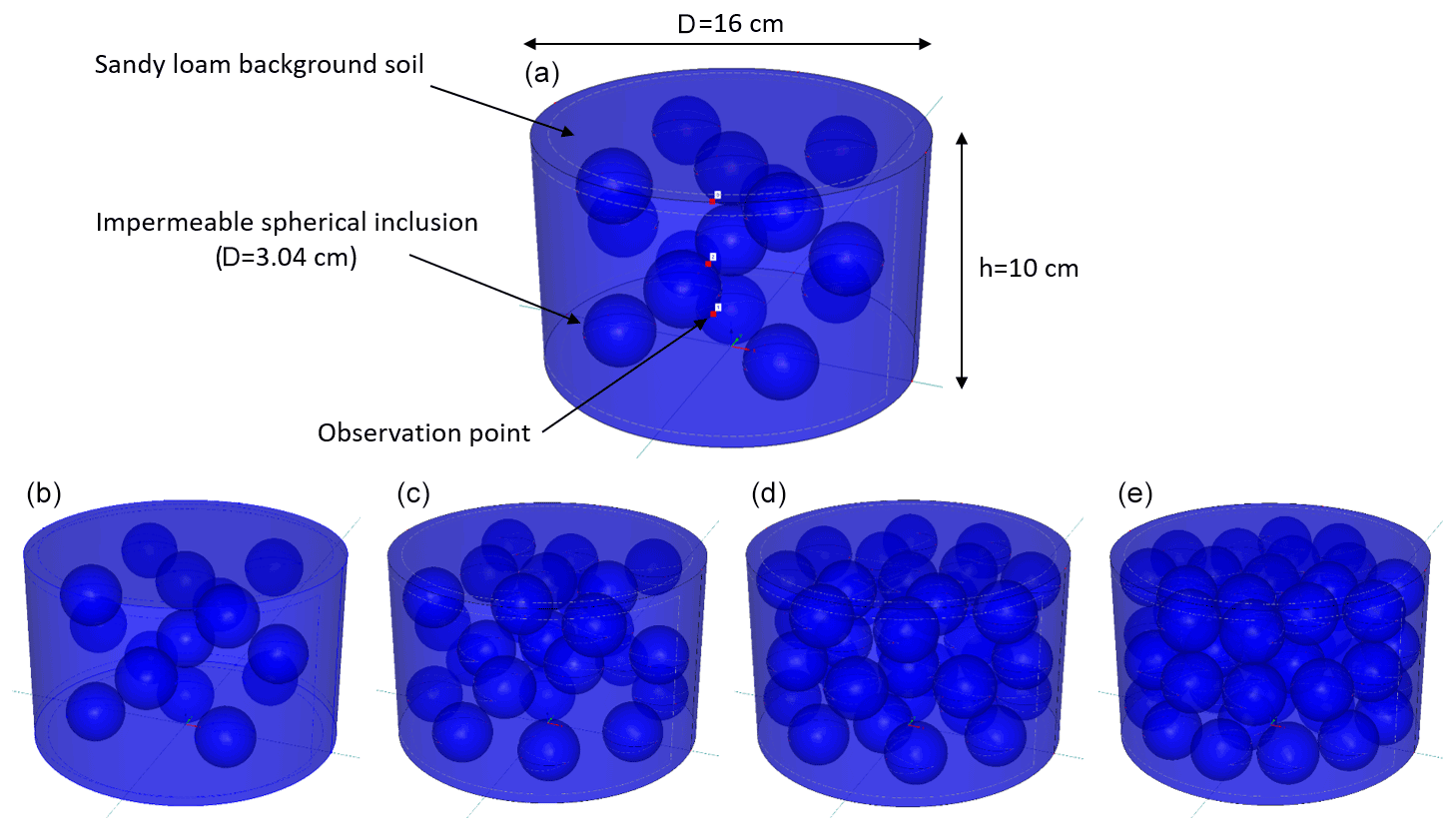
Figure 1Visualization of the generated stony soils in 3D, including the dimension of the RFs and the soil cylinder as well as the location of the observation points (a). The bottom row shows the RF contents of 11.0 % (b), 19.8 % (c), 28.5 % (d), and 37.3 % (e), from left to right.
2.3 Forward simulations
We simulated evaporation (EVA) (Peters and Durner, 2008) and multistep unit-gradient (MSUG) experiments (Sarkar et al., 2019). For EVA, a linear distribution of the pressure head (−2.5 cm top, +7.5 cm bottom) was used as the initial condition. The boundary conditions were no-flux at the bottom, and they were atmospheric with a constant potential evaporation rate of 0.6 (cm d−1) and zero precipitation at the top. The EVA experiments were simulated for 10 d, and the time series of pressure heads at each observation point, the initial volumetric water content, and the cumulative evaporation and evaporation rate were collected for later use in the inverse simulations.
In the virtual MSUG experiment, the soil column was initially fully saturated with a constant pressure head of 0 cm. A sequence of stepwise decreasing constant pressure heads was assigned to the upper and lower boundaries of the column. The duration of the virtual MSUG experiment was 100 d, and the pressure head in the upper and lower boundaries was simultaneously decreased stepwise to a pressure head of −100 cm. The applied pressure heads hi were 0, −1, −3, −10, −20, −30, −60, and −100 cm, respectively. Time steps were chosen such that a steady-state flow condition was reached for each pressure step, indicated by identical water fluxes at the top (inflow) and bottom (outflow) boundaries and constant pressure heads at the observation points. The hydraulic conductivities at the respective pressure heads hi were calculated by dividing the steady-state water flux rates (cm3 d−1) by the total surficial area of the soil column (≈202 cm2).
The converging and diverging flow fields around obstacles produce spatially different pressure heads, even under unit-gradient conditions; as opposed to saturated conditions, these different pressure heads are associated with different water saturations and different local hydraulic conductivities under unsaturated conditions. We were interested in the extent to which this could lead to nonlinear effects in the derivation of the effective hydraulic properties, in particular the effective HCC. Furthermore, as the flow field for a given volume fraction of obstacles depends on dimensionality, i.e., is different in a 2D simulation compared with a 3D simulation, studying the effects in the unsaturated region was one of the main motivations for performing this numerical analysis in 3D.
2.4 Inverse modeling of evaporation in 1D
A 10 d EVA experiment in 1D was simulated with the Hydrus-1D software package (Šimůnek et al., 2006, 2008) to obtain the SHP parameters using inverse modeling. The generated data from the EVA and MSUG forward simulations in 3D were used as input to the 1D inverse simulations. Time series of the pressure heads at three observation depths, mean volumetric water contents in the column during the virtual EVA experiment, and the data points of the effective HCC from the virtual MSUG experiment were used in the objective function. The time series of the mean volumetric water content was calculated from the initial water content, cumulative evaporation, and soil volume. The measurement range for pressure heads used in the objective function was from saturation down to −2000 cm. This reflects a setup with laboratory tensiometers with boiling delay (Schindler et al., 2010). The time series of the simulated evaporation rates from the 3D simulations were used as the time-variable atmospheric boundary condition for the 1D inverse simulations. The 1D soil profile was 10 cm long and was discretized into 100 equally sized finite elements. Similar to the 3D simulations, three observation points were defined at depths of 2.5, 5.0, and 7.5 cm. A no-flux boundary condition was used at the bottom. The six parameters of the van Genuchten model occurring in Eqs. (2) and (3) were all simultaneously estimated by inverse modeling. The weighted least squares objective function was minimized by the Shuffled Complex Evolution algorithm (SCE-UA, Duan et al., 1992). The data obtained from the EVA experiment allow one to identify the WRC from saturation to the pressure where the tensiometers fail as well as the HCC in the middle to dry range of the SHPs (pressure heads of roughly between −100 and −2000 cm), whereas the MSUG provides a precise determination of the HCC in the wet range (Sarkar et al., 2019; Durner and Iden, 2011). The EVA experiments do not provide information on hydraulic conductivity near water saturation (Peters et al., 2015). Therefore, we included the data obtained from the virtual MSUG experiment in the objective function for the inverse simulation of the virtual EVA experiments in order to improve the uniqueness of the inverse solution and the precision of the identified HCC near saturation (see Schelle et al., 2010, for another example).
2.5 Predicting the SHPs of virtual stony soils by scaling models
The SHPs of stony soils obtained by inverse modeling were compared to SHPs that were predicted by available scaling models and used for their evaluation. Considering that f has the dominant influence on the WRC of a stony soil, a common approach is partitioning the WRC and HCC of stony soil based on the volume of each component in the soil–rock mixture and calculating the effective SHPs of stony soil using the volume averaging or the composite-porosity model. The general form of the WRC model considers the moisture contents of the background soil θsoil (h) (cm3 cm−3) and embedded rock fragments θrock (h) (cm3 cm−3) to calculate the effective WRC of stony soils θm (h) (cm3 cm−3) (Flint and Childs, 1984; Peters and Klavetter, 1988) with the following form in the full moisture range (Naseri et al., 2019):
A typical assumption in stony soil hydrology is that the porosity of RFs is negligible. In this case, following Bouwer and Rice (1984), Eq. (4) reduces to
For the effective hydraulic conductivity of stony soils, some scaling models are developed for saturated conditions that might apply to the hydraulic conductivity at any pressure heads. The simplest scaling model accounts only for the reduction in the cross-sectional area available for the flow of water. This leads to the following equation (Ravina and Magier, 1984):
where Kr (–) is the relative hydraulic conductivity of stony soil, i.e., , where Km is the effective hydraulic conductivity of the stony soil (cm d−1), and Ksoil is the conductivity of the background soil (cm d−1).
In a more recent approach, Novák et al. (2011) developed a linear relationship based on the 2D numerical simulation results as a first approximation to scale the saturated hydraulic conductivity of stony soils:
The parameter α was reported to depend on the texture of the background soil, with a range from 1.1 for sandy clay to 1.32 for clay. This model is easy to apply, but it requires the estimation of the parameter α to calculate Kr. For our calculations, we assumed α=1.2 for the sandy loam background soil used in our study.
Another model that has been developed for mixtures with spherical inclusions is the Maxwell model (Maxwell, 1873; Corring and Churchill, 1961; Peck and Watson, 1979; Zimmermann and Bodvarsson, 1995). It takes the value of f, the hydraulic conductivity of the background soil, and the hydraulic conductivity of inclusions into account to calculate the hydraulic conductivity of stony soil. In the special case of impermeable inclusions, the Maxwell model reduces to
A recently developed model by Naseri et al. (2020), which is based on the general effective medium theory (GEM), allows one to consider the effects of the permeability, shape, and orientation of RFs on the effective HCC. For impermeable RFs, the GEM model reduces to the following form:
where fc is the critical f with values between 0.84 and nearly 1, and t is a shape parameter with values between 1.26 and nearly 1.5 for spherical RFs. In this study, we set fc=0.982 () according to the size ratio of the RFs to the background soil, and we set t=1.473 for spherical RFs (for details, see the appendix in Naseri et al., 2020).
It should be noted that all approaches apply at any pressure head hi, i.e., the scaling that is originally developed for saturated conditions with locally constant hydraulic conductivity in the background soil is equally applied to unsaturated conditions.
3.1 Flow field and the variability of state variables in the virtual MSUG experiment
Figure 2 visualizes the pressure head (cm), water content (cm3 cm−3), and velocity (cm d−1) in a 2D cross section in the center of the soil column through the forward simulation of the MSUG experiment. The profile is shown for the steady-state flux situation with a pressure head of −100 cm and stony soil with f=28.5 %. The figure shows a considerable change in the flow velocities, even at the upper boundary. Moreover, as Fig. 2 illustrates, the conditions above an obstacle might be slightly wetter than below an obstacle, but the variations in the pressure head and the water content fields is very small. We note that this general finding was equally applicable for all other pressure head steps in the virtual MSUG experiment.
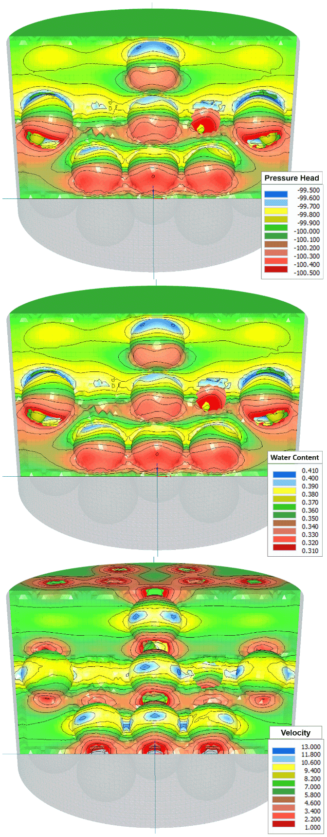
Figure 2Visualization of the pressure head (cm), water content (cm3 cm−3), and velocity (cm d−1) in a 2D profile in the center of the soil column during the forward simulation of the MSUG experiment.
3.2 Comparison of the relative Ks of the scaling models and the 3D simulations under saturated conditions
The dependency of the relative saturated hydraulic conductivity (Kr) on the percentage of RFs, calculated by different scaling models, and the obtained values from the first pressure in the virtual MSUG experiment are presented in Fig. 3. The results of the models are shown up to f=37.3 %, which was the highest value of f simulated in 3D. However, some of the evaluated models are theoretically valid for higher or lower values of f, e.g., 40 % for the Novák et al. (2011) model and higher values for the GEM model (Naseri et al., 2020).
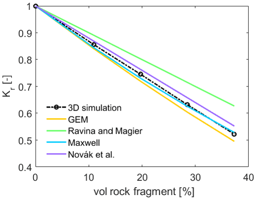
Figure 3Comparison of the values of Kr (–) from the virtual MSUG experiment in 3D (circles) as well as those calculated by different scaling models (solid lines) for f values up to 37.3 %. The dashed line connects the simulated data points of Kr shown by circles.
Obviously, the results of our simulations confirm a linear reduction in Kr with an increasing volume of RFs up to f=37.3 % () in the soil. The numerically obtained values of Kr are shown using circles and are connected by the dashed line in Fig. 3. The dashed line has a slope of −1.29, representing a higher reduction rate of Kr compared with the scaling of Kr that would be proportional to f, which is expressed by Eq. (6) and predicted by the model of Ravina and Magier (1984) (solid green line). This result supports the fact that, even in a stony soil with spherical impermeable RFs, the reduction in the hydraulic conductivity is higher than the reduction in the average cross-sectional area (which is statistically equivalent to the value of f). Hlaváčiková et al. (2016) found an even higher value of −1.45 for spherical RFs with a diameter of 10 cm. The model of Novák et al. (2011) performs better but also leads to a slight underprediction of the reduction in the effective saturated conductivity. The performance of this model could be improved by adjusting the parameter α to match data of the 3D simulation, but doing this would lead to an unfair comparison with the other models. The two models predicting a nonlinear relationship between Kr and f, GEM and Maxwell, show similar results at low RF contents of up to 10 %, with minor differences in the outputs of the models. Among all of the evaluated models for scaling Ks, the Maxwell model yields the closest match to the numerically identified values of Kr.
We note that these results may differ in natural soils, where an increase in the saturated hydraulic conductivity might be expected because of macropore flow in lacunar pores at the interface between the background soil and RFs (Beckers et al., 2016; Hlaváčiková et al., 2016; Arias et al., 2019). We have not included such a process in our 3D simulations.
3.3 Inverse modeling results for effective hydraulic properties
The observed and fitted time series of the pressure heads at the three representative observation points are shown in Fig. 4 for the simulated experiments of the four cases with different values of f. In each case, the fitted pressure heads at the three depths of the column (2.5, 5.0, and 7.5 cm) match well with the time series of the corresponding data from the 3D virtual experiments. Specifically, the match of the pressure heads at 7.5 and 5.0 cm is excellent, whereas there are slight systematic deviations at the uppermost level at the later stage of the virtual EVA experiment.

Figure 4The time series of the 3D-simulated (circles) and 1D-fitted (solid lines) pressure heads at the observation points at three depths of the stony soil columns with the f values of (a) 11.0 %, (b) 19.8 %, (c) 28.5 %, and (d) 37.3 %. The observation depths are indicated using different colors: orange (upper, 2.5 cm), green (middle, 5.0 cm), and blue (lower, 7.5 cm from the top).
Table 1 shows the values of the root-mean-square error (RMSE) and mean absolute error (MAE) between the observed and fitted time series of the pressure heads at three observation points for values of f. According to Table 1, the fit is best for the lower f and in the middle of the column. The highest deviations occur for the highest f, but there is no clear trend. Overall, the RMSE and MAE values are in an acceptable range with respect to the observed values of pressure heads up to −2000 cm. This indicates that the time series of the pressure heads at multiple depths generated by the 3D simulations of the EVA experiments can be described successfully by the 1D Richards equation assuming a homogenous system with effective SHPs.
Table 1The RMSE and MAE values between the observed and fitted pressure heads at three observation points for different values of f.
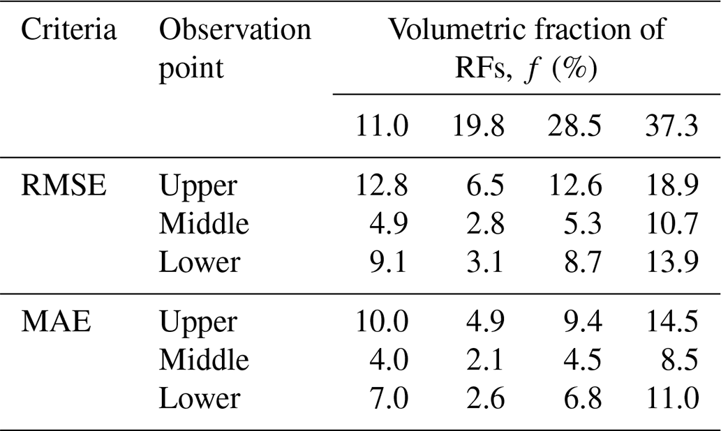
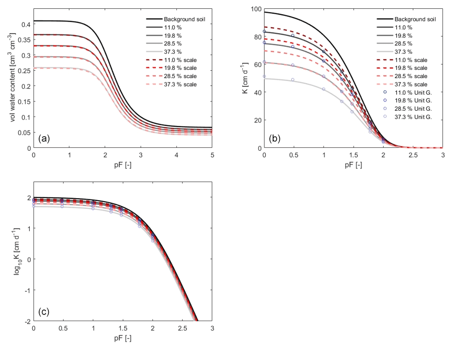
Figure 5The WRCs and HCCs of the background soil (solid black line) and the identified effective WRCs (a) and HCCs (b) of the virtual stony soils (solid gray lines) with different values of f. The HCCs are also presented on a logarithmic scale. The dashed lines show the effective WRCs and HCCs calculated by the models of Bouwer and Rice (1984) and Ravina and Magier (1984). The circles on the HCCs present the data points of hydraulic conductivity obtained by the virtual MSUG experiment under near-saturated conditions up to pF≈2.
The identified SHPs are presented in Fig. 5. The solid lines in the figure show the WRCs and HCCs of the virtual stony soils obtained by inverse simulation (except the solid black lines, which are the WRCs and HCCs of the background soil); the dashed lines represent the WRCs and HCCs scaled using Eq. (5) and Eq. (6), respectively; and the circles on the HCC plots represent the discrete data points of hydraulic conductivity obtained by the virtual MSUG experiment. The WRCs and HCCs are presented on a pF scale, which is defined as pF=log 10(|h|), where h is the pressure head in centimeters (Schofield, 1935). The van Genuchten model parameters of the background soil and stony soils are shown in Table 2.
Table 2The van Genuchten model parameters of the SHPs of the background soil and of the inversely determined effective SHPs of the virtual stony soils with different values of f.

According to Fig. 5 and Table 2, the value of the shape parameter α is independent of the value of f, and the change in the value of n is negligible (but might be systematic). The inversely identified WRC and the predictions from the Bouwer and Rice (1984) scaling model match almost perfectly for all RF contents. In agreement with this, there is also an excellent agreement of the values of the saturated (θs) and residual water contents (θr) (cm3 cm−3) between scaled and identified WRCs. The values of θs and θr in the WRCs are directly related to the values of f, and the respective values of the background soil and the WRC are scaled by this factor over the whole range of the soil water pressure head.
Similar to the WRC, an increase in f reduces the hydraulic conductivity over the whole pressure head range covered by the virtual experiments. However, in contrast to the WRC, the simple scaling model based on Eq. (6) cannot describe the reduction in HCC. Figure 5 shows that the model of Ravina and Magier (1984; dashed lines) underestimates the reduction in the effective HCC for all RF contents. The reason for this might be related to the local variations in the flow velocity in the soil column. It is shown in Fig. 2 that the variations in the water flow velocity might be considerable. The nonlinearities in the flow field and changes in the local conductivities, as well as an increased average flow path length, force a stronger overall conductivity reduction. Thus, the arrangement of RFs might affect the reduction in hydraulic conductivities, leading to different conductivities at the same value of f (Naseri et al., 2020). The degree depends on how the flow area is altered in the soil column due to the presence of RFs (Figs. 1, 2). This result is in agreement with Novák et al. (2011), who reported a higher reduction in conductivity compared with a reduction that is proportional to the RF content. Furthermore, it may also differ depending on the characteristics of RFs, such as their size, shape, and orientation towards flow (Novák et al., 2011).
We had to include the data points of hydraulic conductivity from the virtual MSUG experiment in the inverse objective function to get a precise identification of the HCC obtained by inverse modeling near saturation. The information content from the virtual EVA experiment gives a unique identification only when the flux rate in the system reaches the magnitude of the unsaturated hydraulic conductivity, which is around pF=1.5 to pF=2 for many soils (Peters and Durner, 2008). Although there are some discrepancies visible near saturation for the case with a high value of f, the resulting values of hydraulic conductivity from the virtual MSUG experiment and the inversely identified HCC using the virtual EVA experiment join well around pF=2 for all of the values of f. Therefore, the HCC could be described successfully from the saturation up to pF=3 using the inverse modeling of the virtual EVA experiment with added K support points from the virtual MSUG experiment. The overall results suggest that the effective hydraulic parameters of stony soils could be obtained by the corresponding real experiments, and the result is robust for both WRC and HCC, even if the uncertainty in the identified HCC is higher than that of the WRC (Singh et al., 2020, 2021).
3.4 Evaluation of the Novák, Maxwell, and GEM models using the identified HCC
As stated above, the model of Ravina and Magier (1984), which is a linear scaling approach of the hydraulic conductivity (Eq. 6), underestimates the reduction in conductivity in stony soils. We used the identified HCC as a benchmark to evaluate and compare more advanced models for scaling HCCs, namely the Novák, Maxwell, and GEM models (Eqs. 7, 8, and 9, respectively). Figure 6 illustrates the calculated HCCs of stony soils with different values of f using these models to scale the HCCs and then compares them to the HCC identified by the inverse modeling.
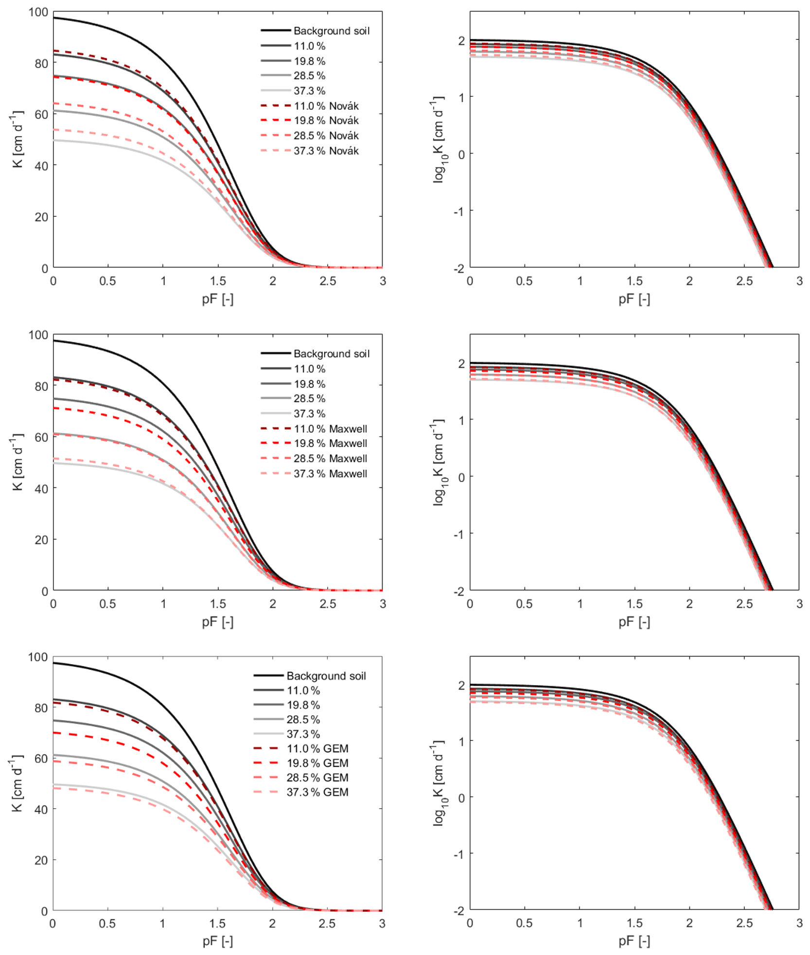
Figure 6Evaluation of the Novák, Maxwell, and GEM models for scaling HCC of stony soils using the identified HCC as a benchmark. In each case, the HCCs were obtained for f = 11.0 %, 19.8 %, 28.5 %, and 37.3 % (). The inverse identified curves are shown using solid lines, and the model results are shown using dashed lines. The value of fc in the GEM model was set as 0.982 with the corresponding shape parameter t = 1.473, and the parameter α=1.2 was selected for the Novák model.
The HCCs calculated by the three models are generally in good agreement with the identified HCC in the observed range of pressure heads. All three models result in a more realistic estimate of the HCC compared with the simple linear scaling approach. While the Novák model slightly underestimates the identified HCC for all four RF contents, the GEM model, in contrast, overestimates the reduction in the hydraulic conductivity. The Maxwell model shows the same results as the GEM model except that it underestimates the HCC for the stony soil with f=37.3 %.
In order to compare the performance of the three models, the average deviation (davg) between the calculated and identified HCCs (logarithmic scale) was calculated to quantify the error of each model in the pF range from 0 to 3 (Table 3). The signs of numbers in Table 3 represent the tendency of the model to over- or underestimate the identified hydraulic conductivities. A negative number means that the model underestimates the reduction in hydraulic conductivity.
Table 3Performance of the Novák, Maxwell, and GEM models quantified by the average deviation hydraulic conductivities (davg) on a logarithmic scale for different values of f.

Table 3 confirms the qualitative tendency toward an underestimation of the conductivity reduction by the Novák model and toward overestimation by the GEM and Maxwell models; however, Table 3 also shows that the difference between the three models is not large and is probably not of relevance in practice (the GEM model at the high value of f, which has the highest deviation, corresponds to a relative mismatch of hydraulic conductivities of about 6 %). Nevertheless, despite the potential of the three models with respect to predicting the HCC of stony soils, we think they require further evaluation using field-measured data of hydraulic conductivity under different experimental conditions.
In this study, we created virtual stony soils with different volumetric fractions of RFs in 3D and identified their effective SHPs from saturation up to pF=3 by inverse modeling of virtual EVA and MSUG experiments in 1D. We used the identified SHPs to investigate the performance of the available scaling models in stony soils, namely the Bouwer and Rice (1984) model for scaling WRCs, and the Ravina and Magier (1984), Maxwell (Peck and Watson, 1979), Novák (Novák et al., 2011), and GEM (Naseri et al., 2020) models for scaling HCCs of stony soils.
Our results show that the boundary fluxes and the internal system states in the virtual 3D EVA experiments, represented by the observed time series of pressure heads at multiple depths, could be matched well by 1D simulations, and the effective WRCs and HCCs of the considered stony soils were determined accurately. Comparison with the scaling models showed that, by assuming a homogeneous background soil and impermeable RFs, the effective WRC can be calculated from the WRC of the background soil using a simple correction factor equal to the volume fraction of background soil, (1−f). This is a result with practical implications for obtaining the WRC of stony soils. In addition, the scaling results for the HCC were promising. Our results confirmed that the reduction in Kr was stronger than that calculated by a simple proportionality to (1−f). The three models of Novák, Maxwell, and GEM consider that, and they performed adequately in predicting the effective HCCs of stony soils. The Maxwell model matched the numerical results best.
Care must be taken before generalizing these results to arbitrary conditions, e.g., highly dynamic boundary conditions with sequences of precipitation and higher and lower evaporation rates, which might yield different results due to the occurrence of nonequilibrium water dynamics and hysteresis. For real stony soils, changes in the pore size distribution of the background soil may result from the presence of RFs (Sekucia et al., 2020), with corresponding consequences for the effective SHPs. This influence was reported to be more common in compactible soils with a shrinkage–swelling potential (Fiès et al., 2002). In highly stony soils, where RFs are not embedded completely in the background soil, the existence of effective SHPs is still an open question. Finally, the impact of arrangement and size of RFs on evaporation dynamics and the effective SHPs needs to be understood. Tackling these problems requires a combination of experimental and modeling approaches.
The software packages used in this study are Hydrus-1D (public domain software) and Hydrus 2D/3D (proprietary). Further software information is available from https://www.pc-progress.com/en/Default.aspx (last access: 3 February 2022) and from the references within the paper (Šimůnek et al., 2006, 2008, 2016).
The Hydrus-3D simulation projects used in this study can be accessed on the research data repository at TU Braunschweig (https://doi.org/10.24355/dbbs.084-202201251240-0, Naseri et al., 2022).
The study was designed by MN, SCI, and WD. MN performed the 3D simulations with Hydrus-3D and drafted the paper. SCI and MN did the inverse simulations. SCI and WD revised the paper and supervised the study.
The contact author has declared that neither they nor their co-authors have any competing interests.
Publisher’s note: Copernicus Publications remains neutral with regard to jurisdictional claims in published maps and institutional affiliations.
The authors appreciate the insightful and constructive comments and remarks from David Dunkerley.
This open-access publication was funded by Technische Universität Braunschweig.
This paper was edited by David Dunkerley and reviewed by two anonymous referees.
Abbasi, F., Jacques, D., Šimůnek, J., Feyen, J., and Van Genuchten, M. T.: Inverse estimation of soil hydraulic and solute transport parameters from transient field experiments: Heterogeneous soil, T. ASAE, 46, 1097, https://doi.org/10.13031/2013.13961, 2003.
Abbaspour, K., Kasteel, R., and Schulin, R.,: Inverse parameter estimation in a layered unsaturated field soil, Soil Sci., 165, 109–123, https://doi.org/10.1097/00010694-200002000-00002, 2000.
Abbaspour, K. C., Sonnleitner, M. A., and Schulin, R.: Uncertainty in estimation of soil hydraulic parameters by inverse modeling: Example lysimeter experiments, Soil Sci. Soc. Am. J., 63, 501–509, https://doi.org/10.2136/sssaj1999.03615995006300030012x, 1999.
Arias, N., Virto, I., Enrique, A., Bescansa, P., Walton, R., and Wendroth, O.: Effect of Stoniness on the Hydraulic Properties of a Soil from an Evaporation Experiment Using the Wind and Inverse Estimation Methods, Water, 11, 440, https://doi.org/10.3390/w11030440, 2019.
Baetens, J. M., Verbist, K., Cornelis, W. M., Gabriëls, D., and Soto, G.: On the influence of coarse fragments on soil water retention, Water Resour. Res., 45, W07408, https://doi.org/10.1029/2008WR007402, 2009.
Ballabio, C., Panagos, P., and Monatanarella, L.: Mapping topsoil physical properties at European scale using the LUCAS database, Geoderma, 261, 110–123, https://doi.org/10.1016/j.geoderma.2015.07.006, 2016.
Beckers, E., Pichault, M., Pansak, W., Degré, A., and Garré, S.: Characterization of stony soils' hydraulic conductivity using laboratory and numerical experiments, SOIL, 2, 421–431, https://doi.org/10.5194/soil-2-421-2016, 2016.
Bouwer, H. and Rice, R. C.: Hydraulic properties of stony vadose zones, Ground Water, 22, 696–705, https://doi.org/10.1111/j.1745-6584.1984.tb01438.x, 1984.
Brakensiek, D. L., Rawls, W. J., and Stephenson, G. R.: Determining the saturated conductivity of a soil containing rock fragments, Soil Sci. Soc. Am. J., 50, 834–835, https://doi.org/10.2136/sssaj1986.03615995005000030053x, 1986.
Celia, M. A., Bouloutas, E. T., and Zarba, R. L.: A general mass-conservative numerical solution for the unsaturated flow equation, Water Resour. Res., 26, 1483–1496, https://doi.org/10.1029/WR026i007p01483, 1990.
Ciollaro, G. and Romano, N.,: Spatial variability of the hydraulic properties of a volcanic soil, Geoderma, 65, 263–282, https://doi.org/10.1016/0016-7061(94)00050-K, 1995.
Coppola, A., Dragonetti, G., Comegna, A., Lamaddalena, N., Caushi, B., Haikal, M. A., and Basile, A.: Measuring and modeling water content in stony soils, Soil Till. Res., 128, 9–22, https://doi.org/10.1016/j.still.2012.10.006, 2013.
Corring, R. L. and Churchill, S. W.: Thermal conductivity of heterogeneous materials, Chem. Eng. Prog., 57, 53–59, 1961.
Corwin, D. L. and Lesch, S. M.: Apparent soil electrical conductivity measurements in agriculture, Comput. Electron. Agr., 46, 11–43, https://doi.org/10.1016/j.compag.2004.10.005, 2005.
Cousin, I., Nicoullaud, B., and Coutadeur, C.: Influence of rock fragments on the water retention and water percolation in a calcareous soil, Catena, 53, 97–114, https://doi.org/10.1016/S0341-8162(03)00037-7, 2003.
Dann, R., Close, M., Flintoft, M., Hector, R., Barlow, H., Thomas, S., and Francis, G.: Characterization and estimation of hydraulic properties in an alluvial gravel vadose zone, Vadose Zone J., 8, 651–663, https://doi.org/10.2136/vzj2008.0174, 2009.
Duan, Q. Y., Gupta, V. K., and Sorooshian, S.,: Shuffled complex evolution approach for effective and efficient global minimization, J. Optimiz. Theory App., 76, 501–521, https://doi.org/10.1007/BF00939380, 1993.
Durner, W. and Flühler, H.: Soil hydraulic properties, in: Encyclopedia of hydrological sciences, edited by: Anderson, M. G. and McDonnell, J. J., chap. 74, 1103–1120. John Wiley & Sons, https://doi.org/10.1002/0470848944.hsa077c, 2006.
Durner, W. and Iden, S. C.: Extended multistep outflow method for the accurate determination of soil hydraulic properties near water saturation, Water Resour. Res., 47, 1–13, https://doi.org/10.1029/2011WR010632, 2011.
Durner, W., Jansen, U., and Iden, S. C.: Effective hydraulic properties of layered soils at the lysimeter scale determined by inverse modelling, Euro. J. Soil Sci., 59, 114–124, https://doi.org/10.1111/j.1365-2389.2007.00972.x, 2008.
Farthing, M. W. and Ogden, F. L.: Numerical solution of Richards' equation: A review of advances and challenges, Soil Sci. Soc. Am. J., 81, 1257–1269, https://doi.org/10.2136/sssaj2017.02.0058, 2017.
Fiès, J. C., Louvigny, N. D. E., and Chanzy, A.: The role of stones in soil water retention, Euro. J. Soil Sci., 53, 95–104, https://doi.org/10.1046/j.1365-2389.2002.00431.x, 2002.
Flint, A. L. and Childs, S.: Development and calibration of an irregular hole bulk density sampler, Soil Sci. Soc. Am. J., 48, 374–378, https://doi.org/10.2136/sssaj1984.03615995004800020030x, 1984.
Germer, K. and Braun J.: Determination of anisotropic saturated hydraulic conductivity of a macroporous slope soil, Soil Sci. Soc. Am. J., 79, 1528–1536, https://doi.org/10.2136/sssaj2015.02.0071, 2015.
Grath, S. M., Ratej, J., Jovičić, V., and Curk, B.: Hydraulic characteristics of alluvial gravels for different particle sizes and pressure heads, Vadose Zone J., 14, 1–18, https://doi.org/10.2136/vzj2014.08.0112, 2015.
Haghverdi, A., Öztürk, H. S., and Durner, W.: Measurement and estimation of the soil water retention curve using the evaporation method and the pseudo continuous pedotransfer function, J. Hydrol., 563, 251–259, https://doi.org/10.1016/j.jhydrol.2018.06.007, 2018.
Hlaváčiková, H. and Novák, V.: A relatively simple scaling method for describing the unsaturated hydraulic functions of stony soils, J. Plant Nutr. Soil Sci., 177, 560–565, https://doi.org/10.1002/jpln.201300524, 2014.
Hlaváčiková, H., Novák, V., and Šimůnek, J.: The effects of rock fragment shapes and positions on modeled hydraulic conductivities of stony soils, Geoderma, 281, 39–48, https://doi.org/10.1016/j.geoderma.2016.06.034, 2016.
Hlaváčiková, H., Novák, V., Kostka, Z., Danko, M., and Hlavčo, J.: The influence of stony soil properties on water dynamics modeled by the HYDRUS model, J. Hydrol. Hydromech., 66, 181–188, https://doi.org/10.1515/johh-2017-0052, 2018.
Hopmans, J. W., Šimůnek, J., Romano, N., and Durner, W.: Inverse Modeling of Transient Water Flow, in: Methods of Soil Analysis, Part 1, Physical Methods, chap. 3.6.2, edited by: Dane, J. H. and Topp, G. C., 3rd edn., SSSA, Madison, WI, 963–1008, https://doi.org/10.2136/sssabookser5.4.c40, 2002.
Kutilek, M.: Soil hydraulic properties as related to soil structure, Soil Till. Res., 79, 175–184, https://doi.org/10.1016/j.still.2004.07.006, 2004.
Lai, J. and Ren, L.: Estimation of effective hydraulic parameters in heterogeneous soils at field scale, Geoderma, 264, 28–41, https://doi.org/10.1016/j.geoderma.2015.09.013, 2016.
Lehmann, P., Bickel, S., Wei, Z., and Or, D.: Physical constraints for improved soil hydraulic parameter estimation by pedotransfer functions, Water Resour. Res., 56, e2019WR025963, https://doi.org/10.1029/2019WR025963, 2020.
Maxwell, J. C.: A Treatise on Electricity and Magnetism, vol. I, reprint: Dover, New York, Sect. 314, p. 440, https://doi.org/10.1038/007478a0, 1873.
Naseri, M., Iden, S. C., Richter, N., and Durner, W.: Influence of stone content on soil hydraulic properties: experimental investigation and test of existing model concepts, Vadose Zone J., 18, 1–10, https://doi.org/10.2136/vzj2018.08.0163, 2019.
Naseri, M., Peters, A., Durner, W., and Iden, S. C.: Effective hydraulic conductivity of stony soils: General effective medium theory, Adv. Water Resour., 146, 103765, https://doi.org/10.1016/j.advwatres.2020.103765, 2020.
Naseri, M., Iden, S. C., and Durner, W.: Evaporation and multi-step unit gradient virtual experiments for 3D geometries of stony soils with different volumes of rock fragments, TU Braunschweig, Institute of Geoecology [data set], https://doi.org/10.24355/dbbs.084-202201251240-0, 2022.
Nasta, P., Huynh, S., and Hopmans, J. W.: Simplified multistep outflow method to estimate unsaturated hydraulic functions for coarse-textured soils, Soil Sci. Soc. Am. J., 75, 418–425, https://doi.org/10.2136/sssaj2010.0113, 2011.
Novák, V. and Hlaváčiková, H.: Applied Soil Hydrology, Springer International Publishing, https://doi.org/10.1007/978-3-030-01806-1, 2019.
Novák, V., Kňava, K., and Šimůnek, J.: Determining the influence of stones on hydraulic conductivity of saturated soils using numerical method, Geoderma, 161, 177–181, https://doi.org/10.1016/j.geoderma.2010.12.016, 2011.
Peck, A. J. and Watson, J. D.: Hydraulic conductivity and flow in non-uniform soil, in: Workshop on Soil Physics and Field Heterogeneity: working papers, Canberra, Australia, CSIRO Division of Environmental Mechanics, 12–14 February 1979, Canberra, 31-9, http://hdl.handle.net/102.100.100/297466?index=1 (last access: 3 February 2022), 1979.
Peters, A. and Durner, W.: Simplified evaporation method for determining soil hydraulic properties, J. Hydrol., 356, 147–162, https://doi.org/10.1016/j.jhydrol.2008.04.016, 2008.
Peters, A., Iden, S. C., and Durner, W.: Revisiting the simplified evaporation method: Identification of hydraulic functions considering vapor, film and corner flow, J. Hydrol., 527, 531–542, https://doi.org/10.1016/j.jhydrol.2015.05.020, 2015.
Peters, R. R. and Klavetter, E. A.: A continuum model for water movement in an unsaturated fractured rock mass, Water Resour. Res., 24, 416–430, https://doi.org/10.1029/WR024i003p00416, 1988.
Ponder, F. and Alley, D. E.: Soil sampler for rocky soils, US Department of Agriculture, Forest Service, North Central Forest Experiment Station, https://doi.org/10.2737/NC-RN-371, 1997.
Radcliffe, D. E. and Šimůnek, J.: Soil physics with HYDRUS: Modeling and applications, CRC press, https://doi.org/10.1201/9781315275666, 2018.
Ravina, I. and Magier, J.: Hydraulic conductivity and water retention of clay soils containing coarse fragments, Soil Sci. Soc. Am. J., 48, 736–740, https://doi.org/10.2136/sssaj1984.03615995004800040008x, 1984.
Russo, D.: Determining soil hydraulic properties by parameter estimation: On the selection of a model for the hydraulic properties, Water Resour. Res., 24, 453–459, https://doi.org/10.1029/WR024i003p00453, 1988.
Sarkar, S., Germer, K., Maity, R., and Durner, W.: Measuring near-saturated hydraulic conductivity of soils by quasi unit-gradient percolation – 1. Theory and numerical analysis, J. Plant Nutr. Soil Sc., 182, 524–534, https://doi.org/10.1002/jpln.201800382, 2019.
Schelle, H., Iden, S. C., Peters, A., and Durner, W.: Analysis of the agreement of soil hydraulic properties obtained from multistep-outflow and evaporation methods, Vadose Zone J., 9, 1080–1091, https://doi.org/10.2136/vzj2010.0050, 2010.
Schelle, H., Durner, W., Schlüter, H., Vogel, H.-J., and Vanderborght, J.: Virtual Soils: Moisture measurements and their interpretation by inverse modeling, Vadose Zone J., 12, 1–12, https://doi.org/10.2136/vzj2012.0168, 2013.
Schindler, U., Durner, W., von Unold, G., and Müller, L.: Evaporation method for measuring unsaturated hydraulic properties of soils: Extending the measurement range, Soil Sci. Soc. Am. J., 74, 1071–1083, https://doi.org/10.2136/sssaj2008.0358, 2010.
Schofield, R. K.: The pF of water in soil, in: Trans. of the Third International Congress on Soil Science, 2, Plenary Session Papers, 30 July–7 August 1935, Oxford, UK, 37–48, https://repository.rothamsted.ac.uk/item/97yx6/the-pf-of-the-water-in-soil (last access: 3 February 2022), 1935.
Sekucia, F., Dlapa, P., Kollár, J., Cerdá, A., Hrabovský, A., and Svobodová, L.: Land-use impact on porosity and water retention of soils rich in rock fragments, Catena, 195, 104807, https://doi.org/10.1016/j.catena.2020.104807, 2020.
Šimůnek, J., Van Genuchten, M. T., and Šejna, M.: The HYDRUS software package for simulating two-and three-dimensional movement of water, heat, and multiple solutes in variably-saturated media, Technical manual, version, 1, 241, PC Progress, Prague, Czech Republic, https://www.ars.usda.gov/research/publications/publication/?seqNo115=204212 (last access: 3 February 2022), 2006.
Šimůnek, J., van Genuchten, M. T., and Šejna, M.: Development and applications of the HYDRUS and STANMOD software packages and related codes, Vadose Zone J., 7, 587–600, https://doi.org/10.2136/vzj2007.0077, 2008.
Šimůnek, J., Van Genuchten, M. T., and Šejna, M.: Recent developments and applications of the HYDRUS computer software packages, Vadose Zone J., 15, 1–25, https://doi.org/10.2136/vzj2016.04.0033, 2016 (code available at: https://www.pc-progress.com/en/Default.aspx, last access: 3 February 2022).
Singh, A., Haghverdi, A., Öztürk, H. S., and Durner, W.: Developing Pseudo Continuous Pedotransfer Functions for International Soils Measured with the Evaporation Method and the HYPROP System: I. The Soil Water Retention Curve, Water, 12, 3425, https://doi.org/10.3390/w12123425, 2020.
Singh, A., Haghverdi, A., Öztürk, H. S., and Durner, W.: Developing Pseudo Continuous Pedotransfer Functions for International Soils Measured with the Evaporation Method and the HYPROP System: II. The Soil Hydraulic Conductivity Curve, Water, 13, 878, https://doi.org/10.3390/w13060878, 2021.
Stevenson, M., Kumpan, M., Feichtinger, F., Scheidl, A., Eder, A., Durner W., and Strauss, P.: Innovative method for installing soil moisture probes in a large-scale undisturbed gravel lysimeter, Vadose Zone J., 20, 1–7, https://doi.org/10.1002/vzj2.20106, 2021.
Tetegan, M., de Forges, A. R., Verbeque, B., Nicoullaud, B., Desbourdes, C., Bouthier, A., Arrouays, D., and Cousin, I.: The effect of soil stoniness on the estimation of water retention properties of soils: A case study from central France, Catena, 129, 95–102, https://doi.org/10.1016/j.catena.2015.03.008, 2015.
Van Genuchten, M. T.: A closed-form equation for predicting the hydraulic conductivity of unsaturated soils, Soil Sci. Soc. Am. J., 44, 892–898, https://doi.org/10.2136/sssaj1980.03615995004400050002x, 1980.
Verbist, K. M. J., Cornelis, W. M., Torfs, S., and Gabriels, D.: Comparing methods to determine hydraulic conductivities on stony soils, Soil Sci. Soc. Am. J., 77, 25–42, https://doi.org/10.2136/sssaj2012.0025, 2013.
Zhang, Y., Zhang, M., Niu, J., Li, H., Xiao, R., Zheng, H., and Bech, J.: Rock fragments and soil hydrological processes: significance and progress, Catena, 147, 153–166, https://doi.org/10.1016/j.catena.2016.07.012, 2016.
Zimmerman, R. W. and Bodvarsson, G.S.: The effect of rock fragments on the hydraulic properties of soils, Lawrence Berkeley Lab., CA, USA, USDOE, Washington, D.C., USA, https://doi.org/10.2172/102527, 1995.