Spherical harmonic covariance and magnitude function encodings for beamformer design

Abstract

Microphone and speaker array designs have increasingly diverged from simple topologies due to diversity of physical host geometries and use cases. Effective beamformer design must now account for variation in the array’s acoustic radiation pattern, spatial distribution of target and noise sources, and intended beampattern directivity. Relevant tasks such as representing complex pressure fields, specifying spatial priors, and composing beampatterns can be efficiently synthesized using spherical harmonic (SH) basis functions. This paper extends the expansion of common stationary covariance functions onto the SHs and proposes models for encoding magnitude functions on a sphere. Conventional beamformer designs are reformulated in terms of magnitude density functions and beampatterns along SH bases. Applications to speaker far-field response fitting, cross-talk cancelation design, and microphone beampattern fitting are presented.

1 Introduction

Acoustic array designs have undergone many iterations of improvement as physical simulation data becomes more accurate and abundant. Rapid microphone and speaker array prototyping efforts have moved into simulation to work in tandem with both industrial and product design. Beamforming sits at the intersection where upstream device geometry and hardware constrain the acoustics and performance of the array, impacting the audio application qualities downstream.

Microphone beamforming improves the signal-to-noise ratio of automatic speech-recognition and wake-word detection [6], estimate source direction-of-arrival [18], and separate acoustic-objects [30]. Speaker beamforming generalizes cross-talk cancelation [34] and can widen acoustic-images by exciting wall reflections [37]. Far-field beamformer performance improves when steering vectors incorporate the local geometry in their free-field acoustic responses [5]. Commercial software such as COMSOL [8] can readily import device geometries in acoustic simulations. Therefore, a common basis representation for beamformer design synthesizes different requirements and simulations across applications.

The complex spherical harmonic (SH) functions [19, 24, 27] form one such basis that have found varied uses for data fitting, analysis, and synthesis. Head-related transfer functions can be efficiently encoded along the SH bases for binaural reproduction [2, 11, 36]. Plane-waves decomposition and beamforming on spherical microphone arrays are directly formulated along the SH bases [9, 21, 25, 27]. For non-spherical arrays, speaker and microphone far-field directivity are decomposed along the SHs from acoustic responses at large finite distances [3] and integrated with room impulse response models [22, 29]. Acoustic directivity can also be fitted to magnitude beampatterns along the SH bases [20, 26].

Magnitude function synthesis on a sphere is less well-known in beamforming but appears in interpolation and Bayesian methods such as Kriging [32] and Gaussian processes [28]. We show how these techniques that specify covariance or kernel functions can relate acoustic directivity with spherical probablistic density functions to better design, fit, and evaluate beampatterns. This improves upon several prototyping stages which we list as the following contributions:

• 1 We fit non-parametric models to acoustic directivity and show that their basis functions can be expanded along SHs to give superior bias-variance trade-offs than spatial cross-correlation models [19] and direct SH fittings [14].

• 2 We derive the analytic SH expansions of several Matérn covariance functions of chordal distances which in previous works have only been shown to be valid on the sphere [12, 13, 16, 31]. Expansion errors under shape-constrained design parameters quickly converges to 0 for increasing max truncation-orders and ensuring model tractability.

• 3 We generalize the acoustic directivity index (DI) [19, 27] to support non-uniform spatial weighting or probability density functions (PDFs) in terms of SHs. This reduces bias of previous discrete sampling schemes that must draw from finite measurements and integrates over target and noise sources’ directional priors indicative of real-world performance compared to flat priors.

• 4 We propose a mixture and product of SH encodings model for synthesizing beampattern targets and accelerate beampattern fitting optimization [20] by analytic derivatives and integration over SH encoded acoustic directivity.

• 5 We present case studies for fitting transcoded SHs to simulated speaker responses’ anechoic acoustic directivity, evaluating expected cross-talk cancelation performances under varying spatial priors, and ranking optimal cross-talk cancelation beampatterns w.r.t. loss functions.

The paper contents are listed as follows: Section 2 introduces the SH notation and derive several useful operators along the SH bases. Section 3 presents novel encodings of Matérn covariance function expansions of chordal distances along the SH bases and proposes the mixture of encodings (MoE) and product of encodings (PoE) models for data fitting and magnitude function synthesis. Section 4 introduces a new probabilistic treatment of DI and then reformulates conventional minimum variance distortionless response (MVDR) and generalized Rayleigh quotient (GRQ) beamformers in terms of SH encoded spatial priors. Section 5 extends beampattern fitting methods such as least squares (LS), magnitude least squares (MLS), and magnitude squared least squares (MSLS) into the SH bases. Section 6 establishes experiments on anechoic far-field directivity fitting by radial basis function (RBF) transcoding, performance impact of spatial priors on cross-talk cancelation, and trade-offs between beampattern fitting methods. Sections 7 and 8 discuss the findings and conclude the work.

2 Background and notation

The spherical harmonics are orthogonal basis functions over spherical coordinates [19]:

$$ \begin{aligned} Y_{l}^{m} (\theta, \phi) & = \sqrt{\frac{(2l + 1)}{4 \pi} \frac{(l-m)!}{(l+m)!}} P_{l}^{m} (\cos \theta) e^{i m \phi}, \\ l & \geq 0, \quad -l \leq m \leq l, \end{aligned} $$

(1)

where for notation, we denote l, m as the order and degree, respectively, (θ, ϕ) the physics convention spherical coordinates for colatitude and azimuth respectively, and $P_{l}^{m} (\cos \theta)$ the associated Legendre polynomials. A function f(θ,ϕ) defined over spherical coordinates can be expanded along the SH bases:

$$ \begin{aligned} f (\theta, \phi) & \approx \sum_{l=0}^{P} \sum_{m=-l}^{l} C_{l}^{m} Y_{l}^{m} (\theta, \phi) = \boldsymbol{C}^{T} \boldsymbol{Y}(\theta, \phi), \\ \boldsymbol{C} & = \left[{C_{0}^{0}, \, C_{1}^{-1}, \, C_{1}^{0}, \, C_{1}^{1}, \, \hdots}\right]^{T}, \\ \boldsymbol{Y}(\theta, \phi) & = \left[{ Y_{0}^{0} (\theta, \phi), \, Y_{1}^{-1} (\theta, \phi), \, Y_{1}^{0} (\theta, \phi), \, \hdots }\right]^{T}, \end{aligned} $$

(2)

where $C_{l}^{m} \in \mathbb {C}$ are the expansion coefficients for basis functions of order l and degree m, and P the maximum order or the number of truncation terms in the SH expansion. The number degrees m for order l totals 2l+1 and number of basis functions upto max truncation-order P is (P+1)². Therefore, a vector of coefficients $\boldsymbol {C} \in \mathbb {C}^{(P+1)^{2} \times 1}$ and SH function evaluations $\boldsymbol {Y}(\theta, \phi) \in \mathbb {C}^{(P+1)^{2} \times 1}$ are denoted in bold and arranged in ascending basis orders [19]. We derive several vector operators along the SH coefficients of f(θ,ϕ) from Eq. 2.

Conjugation: The complex conjugate ()^∗ of function f(θ,ϕ) flips the order of m and negates odd m harmonics using the conjugate SH property $Y_{l}^{m*}(\theta, \phi) = (-1)^{m} Y_{l}^{-m}(\theta, \phi)$ in [27]. The vectorized formulation permutes the SH coefficients

$$ \begin{aligned} f^{*}(\theta, \phi) & \approx \widetilde{\boldsymbol{C}}^{T} \boldsymbol{Y}(\theta, \phi), \quad \widetilde{\boldsymbol{C}} = \mathbf{diag}\left[{\boldsymbol{D}_{0 \hdots P}}\right] \, \boldsymbol{C}^{*}, \\ \boldsymbol{D}_{l} & = \boldsymbol{J}_{l} \, \mathbf{diag}\left[{(-1)^{-l : l}}\right], \end{aligned} $$

(3)

via the exchange matrix $\boldsymbol {J}_{l} \in \mathbb {R}^{(2 l + 1) \times (2 l + 1) }$ defined in [15]. A real-valued function f(θ,ϕ)=f^∗(θ,ϕ) therefore has SH coefficients satisfying $\boldsymbol {C} = \widetilde {\boldsymbol {C}}$.

Multiplication: The product two SH basis function is closed under addition

$$ \begin{aligned} Y_{l}^{m}(\theta, \phi) Y_{\bar{l}}^{\bar{m}}(\theta, \phi) & = \sum_{L=\left|{l - \bar{l}}\right|}^{\left|{l + \bar{l} }\right|} \sqrt{\frac{(2 l + 1) (2 \bar{l} + 1) }{4 \pi (2L + 1)}} Y_{L}^{M} (\theta, \phi) \\ & \times c \left({\begin{array}{ccc} l, \bar{l}, L \\ m, \bar{m}, M \end{array}}\right) c \left({\begin{array}{ccc} l, \bar{l}, L \\ 0, 0, 0 \end{array}}\right), \\ \end{aligned} $$

(4)

where $M = m + \bar {m}$ and c() the Clebsch-Gordan coefficients defined in [4, 10]. We can therefore expand the product of functions $f(\theta, \phi) \approx \boldsymbol {C}_{f}^{T} \boldsymbol {Y}(\theta, \, \phi), \, \boldsymbol {C}_{f} \in \mathbb {C}^{(P+1)^{2} \times 1}$ and $\bar {f}(\theta, \phi) \approx \boldsymbol {C}_{\bar {f}}^{T} \boldsymbol {Y}(\theta, \, \phi), \, \boldsymbol {C}_{\bar {f}} \in \mathbb {C}^{(\bar {P} + 1)^{2} \times 1}$ in terms of a product operator ◇ of SH coefficients

$$ \begin{aligned} & \diamond : \, \boldsymbol{C}_{f} \times \boldsymbol{C}_{\bar{f}} \rightarrow \boldsymbol{C}_{f \bar{f}}, \\ f(\theta, \phi) \bar{f}(\theta, \phi) & \approx (\boldsymbol{C}_{f} \, \diamond \, \boldsymbol{C}_{\bar{f}})^{T} \boldsymbol{Y}(\theta, \, \phi), \\ (\boldsymbol{C}_{f} \, \diamond \, \boldsymbol{C}_{\bar{f}})_{L}^{M} & = \sum_{l = 0}^{P} \sum_{\bar{l} =\bar{l}_{0}}^{\bar{l}_{1}} \sqrt{\frac{(2 l + 1) (2 \bar{l} + 1) }{4 \pi (2L + 1)}} \, c \left({\begin{array}{ccc} l, \bar{l}, L \\ 0, 0, 0 \end{array}}\right) \\ &\times \sum_{m = m_{0} }^{m_{1}} c \left({\begin{array}{ccc} l, \bar{l}, L \\ m, \bar{m}, M \end{array}}\right) C_{l}^{m} \bar{C}_{\bar{l}}^{\bar{m}}, \\ \bar{l}_{0} & = \left|{L - l}\right|, \quad \bar{l}_{1} = \min(\left|{L + l}\right|, \bar{P}), \\ m_{0} & = \max(M - \bar{l}, -l), \quad m_{1} = \min(M + \bar{l}, l), \end{aligned} $$

(5)

where L, M are indices for the order and degree respectively, $\bar {m} = M - m$, and $C_{l}^{m} \in \boldsymbol {C}_{f}, \bar {C}_{\bar {l}}^{\bar {m}} \in \boldsymbol {C}_{\bar {f}}, \boldsymbol {C}_{f\bar {f}} \in \mathbb {C}^{(P + \bar {P} + 1)^{2} \times 1}$.

Squared modulus: A function’s magnitude squared can be computed along SH bases via the product operator of the SH expansion with its conjugate in Eqs. 3 and 5 given by

$$ \begin{aligned} \left|{ f(\theta, \phi) }\right|^{2} = f(\theta, \phi) \, f^{*}(\theta, \phi) \approx (\boldsymbol{C} \diamond \boldsymbol{\widetilde{C}})^{T} \boldsymbol{Y}(\theta, \, \phi). \end{aligned} $$

(6)

3 Function encodings and fitting

We define a stationary covariance function K over random variables X(r) that depends only on the chordal distance d(Θ) on a unit sphere:

$$ \begin{aligned} K(X(\boldsymbol{r}), X(\boldsymbol{r'})) & = \mathbb{E} \left[{ X(\boldsymbol{r}) X^{*}(\boldsymbol{r'})}\right] = K(d(\Theta)), \\ d(\Theta) & = 2 \sin {\frac{\Theta}{2}} = \left\lVert{\boldsymbol{r} - \boldsymbol{r'}}\right\rVert, \end{aligned} $$

(7)

where $\boldsymbol {r} \in \mathbb {R}^{3}$ is a cartesian unit vector representing a direction or point on the unit sphere, and Θ= cos−1(r·r^′) the central angle between r,r^′.

As a motivating example, let the random variable X(r) be the sound pressure P(r,Ω,k) at position r and wave number k due to a unit amplitude wave incident to a direction drawn from random variable Ω with uniform density function f(Ω)=(4π)⁻¹ over the unit sphere. This is equivalent to the well-known spatial cross-correlation between sound pressure at two points in a diffuse field [19] which after substitution into Eq. 7 yields the unnormalized sinc kernel:

$$ \begin{aligned} \int_{\Omega} \frac{\mathrm{P} (\boldsymbol{r}, \Omega, k) \mathrm{P}^{*} (\boldsymbol{r'}, \Omega, k)}{4\pi} d \Omega = \frac{\sin (k \left\lVert{\boldsymbol{r} - \boldsymbol{r'}}\right\rVert)}{k \left\lVert{\boldsymbol{r} - \boldsymbol{r'}}\right\rVert}, \end{aligned} $$

(8)

where the positive semi-definiteness follows from expanding P(r,Ω,k)P^∗(r^′,Ω,k) along SHs in [19] to supply the weights λ and orthonormal bases ψ to Mercer’s Theorem $K(\boldsymbol {r}, \boldsymbol {r'}) = \sum _{l=0}^{\infty } \lambda _{l} \psi _{l} (\boldsymbol {r}) \psi _{l} (\boldsymbol {r'})$ [23]. Moreover, Mercer’s theorem allows a valid covariance function to be defined without explicit specification of its random variables X(r) provided that the former is expressible along an orthonormal bases such as the SHs. We derive the analytic SH expansions of several well-known stationary covariance functions or RBFs.

3.1 Analytic encodings

Stationary covariance functions can be expanded into the SH domain via the Legendre addition theorem:

$$ \begin{aligned} K(\Theta, \, \ell) & = \sum_{l=0}^{\infty} b_{l} (g, \, \ell) P_{l}(\cos \Theta), \\ P_{l}(\cos \Theta) & = \frac{4 \pi}{ 2 l + 1} \sum_{m = -l}^{l} Y_{l}^{m*} (\theta, \phi) \,Y_{l}^{m*} (\theta_{*}, \phi_{*}), \end{aligned} $$

(9)

where expansion weights b_l(g, ℓ) belong to some function g parameterized by ℓ. The Legendre polynomial P_l(cosΘ) of the angular distance 0≤Θ≤π is expanded into products of SHs evaluated at free coordinates (θ, ϕ) w.r.t. a center or fixed coordinate (θ_∗, ϕ_∗). The SH coefficients after substituting Eq. 9 into 2 are given by

$$ \begin{aligned} C_{l}^{m} (\Xi) & = \frac{4 \pi \, b_{l}(g, \, \ell) }{ 2 l + 1} \,Y_{l}^{m*} (\theta_{*}, \phi_{*}), \\ f(\theta, \phi, \, \Xi) & = \boldsymbol{C}^{T}_{\Xi} \boldsymbol{Y}(\theta, \phi), \quad \Xi = \left\{\theta_{*}, \, \phi_{*}, \, g, \, \ell\right\}, \\ \end{aligned} $$

(10)

where Ξ is the set of parameters and $\boldsymbol {C}^{T}_{\Xi }$ the vector of coefficients $C_{l}^{m} (\Xi)$. The function specific weights b_l(g, ℓ) must be real-valued and depend only on the order l as the conjugate SH property in Eq. 3 ensures that $f(\theta, \phi, \, \Xi) \in \mathbb {R}$ iff $\boldsymbol {C}^{T}_{\Xi } = \widetilde {\boldsymbol {C}}^{T}_{\Xi }$. The exact values of b_l(g, ℓ) can be computed via the sine expansion of the Legendre polynomials [16, 31] given by

$$ \begin{aligned} b_{l}(g, \, \ell) & = \frac{2 l + 1}{2} \sum_{k=0}^{\infty} D_{l}^{k} A_{l}^{k}(g, \, \ell), \\ D_{l}^{k} &= \frac{4}{\pi} \frac{\prod [2(1:l), \, 2(1:k) - 1, \, l + (1:k)]} {\prod [2(1:l) + 1, \, (1:k), \, 2(l + (1:k)) + 1]}, \\ A_{l}^{k}(g, \, \ell) &= \frac{1}{2} \left({g(l + 2 k, \, \ell) - g(l + 2k + 2, \, \ell)}\right), \\ g(n, \ell) & = \int_{0}^{\pi} K(\Theta, \, \ell) \cos (n \Theta) \, d \Theta, \end{aligned} $$

(11)

where expansion coefficients g(n,ℓ) integrate the product of covariance function K and the Chebyshev polynomials cos(nΘ)=T_n(cosΘ).

We now consider members of the family of half-integer order Matérn covariance functions [1] of chordal distances d(Θ) in Eq. 7 given by

$$ \begin{aligned} K_{\nu}(t, \, \ell) & = e^{-s t} \frac{\Gamma(p+i) }{\Gamma(2p+i)} \sum_{i=0}^{p} \frac{(p+1)!}{i!(p-1)!} \left({2 s t}\right)^{i}, \\ \nu & = p + 1/2, \quad t = d(\Theta), \quad s = \frac{ \sqrt{2 \nu}}{\ell}, \end{aligned} $$

(12)

where $p \in \mathbb {N}^{+}$ and Γ() is the Gamma function. These RBFs are products of the Laplace kernel and polynomial functions which can be combined with the Chebyshev polynomials after a change of variables

$$ \begin{aligned} \cos (n \Theta) & = \cos \left({2n \frac{\Theta}{2}}\right) = T_{2n} \left({\cos \frac{\Theta}{2}}\right) \\ & = F \left({[2n,\, -2n], \frac{1}{2}, \frac{1 - \cos \frac{\Theta}{2}}{2}}\right) \\ & = F \left({\left[{\frac{1}{2} + n,\, \frac{1}{2} - n}\right], \frac{1}{2}, \sin^{2} \frac{\Theta}{2}}\right) \cos {\frac{\Theta}{2}} \\ & = F \left({\left[{\frac{1}{2} + n,\, \frac{1}{2} - n}\right], \frac{1}{2}, \frac{t^{2}}{4}}\right) \frac{\partial t}{\partial \Theta}, \end{aligned} $$

(13)

where F(a,b,z) is the generalized hypergeometric function (see Appendix Eq. 48). The modified integral after substituting Eqs. 12 and 13 into g(n,ℓ) is given by

$$ \begin{aligned} g_{\nu}(n, \ell) &= \int_{0}^{2} K_{\nu} (t, \ell) F\left({\left[{\frac{1}{2} + n, \frac{1}{2} - n}\right], \frac{1}{2}, \frac{t^{2}}{4}}\right) d t, \end{aligned} $$

(14)

where $dt = \cos {\frac {\Theta }{2}} \, d \Theta$. After symbolic integration [35] w.r.t. t for cases $\nu = \left \{\frac {1}{2}, \frac {3}{2}, \frac {5}{2}, \infty \right \}$, the novel expansion coefficients are presented as follows:

Matérnν=1/2 (Exponential): Non-differentiable function at Θ=0.

$$ \begin{aligned} K_{\frac{1}{2}}(\Theta, \, \ell) & = e^{-\frac{t}{\ell}}, \quad \xi = \ell^{-2}, \\ g(n, \ell) & = (-1)^{n} \pi (F(1, \left[{1-n, 1+n}\right], \xi) \\ & - \ell^{-1} F(1, [3/2-n, 3/2+n], \xi)). \end{aligned} $$

(15)

Matérnν=3/2: Once-differentiable product of linear polynomial and exponential functions.

$$ \begin{aligned} K_{\frac{3}{2}}(\Theta, \, \ell) &= \left({1 + \frac{\sqrt{3} t}{\ell}}\right) e^{-\frac{\sqrt{3} t}{\ell} }, \quad \xi = 3 \ell^{-2}, \\ g(n, \ell) & = (-1)^{n} \pi (F(1, [1-n, 1+n], \xi) \\ & - 2 \xi F(2, [2-n, 2+n], \xi) \\ & + \frac{2 \xi \sqrt{3}}{\ell} F(2, [5/2-n, 5/2+n], \xi)). \end{aligned} $$

(16)

Matérnν=5/2: Twice-differentiable product of quadratic polynomial and exponential function.

$$ \begin{aligned} K_{\frac{5}{2}}(\Theta, \, \ell) & = \left({1 + \frac{\sqrt{5} t}{\ell} + \frac{5 t^{2}}{3 \ell^{2}}}\right) e^{-\frac{\sqrt{5} t}{\ell}}, \quad \xi = 5 \ell^{-2}, \\ g(n, \ell) & = (-1)^{n} \pi (F([1], [1-n, 1+n], \xi) \\ & -2 \xi F(2, [2-n, 2+n], \xi) \\ & + \frac{2 \xi \sqrt{5}}{\ell} F(2, [5/2-n, 5/2+n], \xi) \\ & + \frac{2 \xi \sqrt{\pi} }{3} F([3/2, 2], [1/2, 2-n, 2+n], \xi) \\ & - \frac{ \xi \sqrt{5 \pi}}{\ell} F([2, 5/2], [3/2, 5/2\!-n, 5/2+n], \xi)). \end{aligned} $$

(17)

Matérnν=∞ (squared exponential): Infinitely differentiable function everywhere.

$$ \begin{aligned} K_{\infty}(\Theta, \, \ell) & = e^{-\frac{t^{2}}{2 \ell^{2}}}, \quad \xi = \ell^{-2}, \\ g(n, \ell) & = \pi e^{- \xi} I_{n}(\xi), \end{aligned} $$

(18)

where I_n is the nth order modified Bessel function of the first kind.

Design parameters: The bandwidth term ℓ which parameterizes the RBFs can be chosen to satisfy constraints such as the full width at half magnitude (FWHM) and the minimum. The FWHM for RBFs on the sphere gives twice the radians at which the function is half the maximum amplitude ($K_{\nu }(\Theta, \ell) = \frac {1}{2}$) and minimized at Θ=π as shown in Fig. 1. For Matérn covariance functions, the FWHM can be found for a given ℓ and conversely, ℓ for a desired target response:

$$ \begin{aligned} \textrm{FWHM}_{\nu}(\ell) & = 2 \arg\underset{\Theta}{\min} \left|{K_{\nu}(\Theta, \, \ell) - \frac{1}{2}}\right|, \\ \ell_{\nu} (T_{\Theta}, \, T_{{dB}}) & = \arg\underset{\ell}{\min} \left|{K_{\nu}(T_{\Theta}, \, \ell) -10^{\frac{T_{{dB}}}{20}}}\right|, \end{aligned} $$

(19)

Fig. 1

Solid lines show RBFs with FWHM $\frac {2 \pi }{3}$ and bandwidth terms ℓ that satisfy $K_{\nu }(\Theta = \frac {\pi }{3}, \ell) = \frac {1}{2}$. Dashed lines show RBFs with $\ell _{\nu } \left (\Theta = \frac {\pi }{3}, \, T_{{dB}} = -12\right)$ for Eq. 19. Smaller ℓ and larger ν result in more localized covariance functions

where T_dB is the target decibel response at T_Θ radians (See Appendix Eqs. 50–55 for analytic expressions).

For specifying sharp peaks and discontinuities on a sphere, a sharp covariance function is desirable. Given Matérn functions of different classes $K_{\nu _{1}}, K_{\nu _{2}}$ where ν₁<ν₂ and identical FWHM, the less differentiable function $K_{\nu _{1}}$ is bounded above for $0 < \Theta < \frac {\textrm {FWHM}}{2}$ and below for $\frac {\textrm {FWHM}}{2} < \Theta < \pi$ as shown in Fig. 1. A sharp peak function can therefore be parameterized with small ν,T_dB and T_Θ but requires higher max truncation-order terms P or SH bases to achieve the same reconstruction error as shown in Fig. 2. The root mean square error (RMSE) curve RMSE(P) is asymptotically steeper for smoother function classes (larger ν) and bounded below by functions with larger bandwidth ℓ within the same class. We now propose new techniques for fitting SH encoded RBFs to far-field directivity responses and composing magnitude functions on the sphere.

Fig. 2

RBFs with design parameters in Fig. 1 are expanded at (θ=0, ϕ=0) along SH bases in Eqs. 9 and 10 upto maximum truncation-order P. Their expansions are evaluated over the domain of |θ|≤π, ϕ=0 (elevation) in Eq. 2 and the root mean square errors computed

3.2 Mixture of encodings

A set of M complex target responses (X_i, θ_i, ϕ_i) can be modeled by a weighted summation of N distinct SH encoded functions f(θ, ϕ, Ξ_j) in Eq. 10 given by

$$ \begin{aligned} f(\theta, \phi) = c + \sum^{N}_{j=1} w_{j} f(\theta, \, \phi, \, \Xi_{j}), \end{aligned} $$

(20)

where c is a scalar constant, and w_j are unknown weights. The system of equations is given by

$$ \begin{aligned} \boldsymbol{A} \boldsymbol{w} & = \boldsymbol{b} - \boldsymbol{c}, \quad A_{{ij}} = f(\theta_{i}, \, \phi_{i}, \, \Xi_{j}), \quad b_{i} = X_{i}, \\ \Xi_{j} & = \left\{\theta_{*j}, \, \phi_{*j}, \, g_{j}, \, \ell_{j}\right\}, \quad \boldsymbol{c} = c \times \boldsymbol{1}, \end{aligned} $$

(21)

where $\boldsymbol {A} \in \mathbb {C}^{M \times N}, \boldsymbol {w} \in \mathbb {C}^{N \times 1}, \boldsymbol {b}, \, \boldsymbol {c} \in \mathbb {C}^{M \times 1}$ are the system matrix, vectorized unknowns, targets, and scalar constant respectively. The SH expansion of a constant over spherical coordinates is given by $2 c \sqrt {\pi } \, Y_{0}^{0} (\theta, \phi)$. The solution vector w can be found by direct inversion of A when N=M and by least-squares methods for overdetermined cases N<M or when constraints on w are specified.

For N=M and common RBF parameterizations Ξ_i={θ_i, ϕ_i, g, ℓ} centered over distinct target responses (X_i, θ_i, ϕ_i), MoE converges to RBF interpolation for valid kernel functions as the max truncation-order P increases; SH encodings converge to covariance functions at the limit ${\lim }_{P \to +\infty } f(\theta _{i}, \, \phi _{i}, \, \Xi _{j}) = K_{\nu }(\Theta _{{ij}}, \ell _{j})$. Moreover, SH encodings for arbitrary P are valid kernels as the Legendre polynomials in Eq. 9 are also valid kernels [16]. As a result, the original kernel functions can be initially fitted to a large number of samples using the original kernel functions before expanding into the SH bases. For example, native methods such as Gaussian processes [28] use the log-marginal likelihood to fit bandwidth ℓ and specify the posterior mean weights

$$ \begin{aligned} \boldsymbol{w} = (\boldsymbol{K} + \sigma^{2} \boldsymbol{I})^{-1} (\boldsymbol{b} - \boldsymbol{c}), \quad \boldsymbol{K}_{{ij}} = K_{\nu}(\Theta_{{ij}}, \ell), \end{aligned} $$

(22)

computed from a common covariance function where Θ_ij is the central angle between (θ_i,ϕ_i) and (θ_j,ϕ_j). We refer to this schema as MoE-RBF transcoding given that a non-parametric RBF interpolation of N supports is encoded rather than fitted to (P+1)² SH basis functions. The bias-variance trade-off after transcoding is thus more sensitive to the choice of the kernel function and its smoothness and locality on the sphere rather than the number of SH bases (See Section 6.1 for experiment).

We now consider the case where non-negative RBFs are fitted to magnitude only responses X≥0. At the limit where P→∞ and f(θ_i, ϕ_i, Ξ_j)=K_ν(Θ_ij,ℓ_j), the interpolant f(θ,ϕ) can be constrained to be non-negative by finding the non-negative least-squares solution w to the real-values of Eq. 21 given by

$$ \begin{aligned} \mathbb{R} \left[{\boldsymbol{A}}\right] \mathbf{diag} \left[{ \mathbf{sgn} (\mathbb{R}[\boldsymbol{b} - \boldsymbol{c}])}\right] \boldsymbol{w} & = \mathbb{R} \left[{\boldsymbol{b} - \boldsymbol{c}}\right], \end{aligned} $$

(23)

where c=0 and w≥0. For finite order SH encodings however, f(θ_i, ϕ_i, Ξ_j) and f(θ,ϕ) may ripple below 0 due to truncation error. If constant c>0 is raised, then the sign of $\mathbb {R}[\mathbf {b} - \boldsymbol {c}]$ forces each encoding f(θ, ϕ, Ξ_i) to contribute as either a peak or a null (See example in Fig. 3a) and the latter may overshoot and induce negative values in f(θ,ϕ). One solution is to fit SH encodings of a kernel’s squared modulus from Eq. 6 with non-negative weights w≥0 given by

$$ \begin{aligned} f(\theta, \, \phi, \, \Xi_{j}) & = \left|{\bar{f}(\theta, \, \phi, \, \Xi_{j})}\right|^{2}, \quad c = 0, \end{aligned} $$

(24)

Fig. 3

Mixture and product of two K_∞ kernels from Eqs. 23, 28. Weights w are fitted to X={12_dB, −12_dB} responses respectively at their centers of expansion (θ_∗, ϕ_∗). Only the magnitude responses are shown as the phase component is constant (0 radians)

where $\bar {f}(\theta, \, \phi, \, \Xi _{j})$ is an SH encoding of a kernel and its squared modulus is strictly non-negative and does not ripple below 0. We note that a kernel’s squared modulus is a valid kernel due to the general rule that the product of kernels is a kernel [28]. All modulus squared Matérn kernels are thereby suitable candidates for magnitude fitting with slight modifications to parameter selection.

Parameter optimization of ℓ depends on the Matérn class ν; exponential and squared exponential $K_{\frac {1}{2}}(\Theta, \ell) = \left |{K_{\frac {1}{2}}(\Theta, 2 \ell)}\right |^{2}, K_{\infty }(\Theta, \ell) = \left |{K_{\infty }(\Theta, \ell \sqrt {2})}\right |^{2}$ are closed under the squared modulus and so bandwidth ℓ is simply scaled. For other half-integer ν classes, the kernels remain products of exponential and polynomial functions but are not part of the Matérn family; bandwidth ℓ needs re-derivation w.r.t. the objective function. For parameter design of ℓ, targeting half the desired dB response T_dB/2 at T_Θ in Eq. 19 is sufficient.

3.3 Product of encodings

The PoE model or the product of N SH encodings is useful for fitting to low-order target responses given by

$$ \begin{aligned} f(\theta, \phi) = \prod_{j = 1}^{N} (1 + w_{j} f(\theta,\, \phi, \, \Xi_{j})), \end{aligned} $$

(25)

where $w_{j} \in \mathbb {C}$ are unknown weights and the product of SH encodings 1+f(θ, ϕ, Ξ_j) are closed under SH multiplication via Eq. 5; SH expansion of the unit constant is $2 \sqrt {\pi } \, Y_{0}^{0} (\theta, \phi)$. PoEs can model sharper functions than MoEs (See example in Fig. 3b) as the derivative of products are multiplicative whereas the derivative of mixtures is additive. PoEs however do require substantially more bases than MoE as the product of N SH encodings of Pth max truncation-order spans (NP+1)² bases. Data fitting is also not closed-form due to non-linear objective functions.

Consider the non-linear least-squares solution that minimizes the surrogate log function

$$ \begin{aligned} L(\mathbf{w}) &= \left | \left | \sum_{i = 1}^{M} F_{i}^{2}(\boldsymbol{w}) \right | \right |_{2}^{2}, \quad b_{i} = X_{i}, \\ F_{i}(\boldsymbol{w}) & = \sum_{j=1}^{N} \log \left (1 + w_{j} \, f(\theta_{i}, \, \phi_{i}, \, \Xi_{j}) \right) - \log b_{i}, \end{aligned} $$

(26)

where (X_i, θ_i, ϕ_i) are the M target responses. For gradient-based optimization, the Jacobian given by

$$ \begin{aligned} \frac{\partial F_{i}(\boldsymbol{w})}{\partial w_{j}} = \frac{f(\theta_{i}, \, \phi_{i}, \Xi_{j})}{1 + w_{j} \, f(\theta_{i}, \, \phi_{i}, \, \Xi_{j}) }, \end{aligned} $$

(27)

can be used to update w.

In the case of magnitude target responses, a non-negative PoE can be fitted by constraining the weights to be real and bounded w_j≥−1. For the case of N=M, the weights can be further constrained such that each encoding contributes a peak or null to f(θ,ϕ) analogous to the MoE formulation in Eq. 23:

$$ \begin{aligned} f(\theta, \phi) & = \prod_{j=1}^{N} (1 + w_{j} \, \mathbf{sgn} (b_{j} - 1) f(\theta,\, \phi, \, \Xi_{j})), \\ & 0 \leq w_{j} \leq 1, \quad \forall \, \, \mathbf{sgn} (b_{j} - 1) = -1, \\ & 0 \leq w_{j} \leq \infty, \quad \forall \, \, \mathbf{sgn} (b_{j} - 1) = 1, \\ \end{aligned} $$

(28)

where $f(\theta, \phi, \Xi _{j}) = \frac {\bar {f}(\theta, \phi, \Xi _{j})}{\bar {f}(\theta _{j}, \phi _{j}, \Xi _{j})}$ normalize SH encodings $\bar {f}(\theta, \phi, \Xi _{j})$ of kernels at their center of expansions (θ_j,ϕ_j) to prevent over-shooting. PoEs can therefore model low-order cascades of spatial peak and null magnitude functions. We now show how to extend MoE and PoE models into beamformer designs.

4 Conventional beamformer extensions

An N channel array can be oriented towards directional sources by parameterizing so-called steering vectors in terms of each channel’s directivity or anechoic far-field responses. A steering vector d(θ, ϕ) and the resulting beampattern B(θ,ϕ) can be parameterized along SH bases given by

$$ \begin{aligned} \boldsymbol{d}(\theta, \phi) & = \boldsymbol{C}^{T}_{d} \boldsymbol{Y}(\theta, \phi), \, \, \, \, B(\theta, \phi) = \boldsymbol{w}^{H} \boldsymbol{d}(\theta, \phi), \end{aligned} $$

(29)

where $\boldsymbol {C}_{d} \in \mathbb {C}^{(P+1)^{2} \times N}$ is the column matrix of SH coefficients fitted to N sets of acoustic directivities, and $\boldsymbol {w} \in \mathbb {C}^{N \times 1}$ are the unknown beamformer’s weights. The beamformer’s DI evaluates the power output gain at (θ_∗,ϕ_∗) w.r.t. the power average over the spherical coordinates [19, 27]:

$$ \begin{aligned} \text{DI}(B(\theta_{*}, \phi_{*})) & = \frac{4 \pi \, \left|{B}\right|^{2}(\theta_{*}, \phi_{*}) }{\int_{\Omega} \left|{B}\right|^{2}(\theta, \phi) \, d \Omega} \\ &= \frac{4 \pi \, \left|{\boldsymbol{w}^{H} \boldsymbol{C}^{T}_{d} \boldsymbol{Y}(\theta_{*}, \phi_{*})}\right|^{2} }{\boldsymbol{w}^{H} \boldsymbol{C}^{T}_{d} \boldsymbol{C}_{d}^{*} \boldsymbol{w} }. \end{aligned} $$

(30)

Maximizing DI is the basis of conventional beamformers such as MVDR which we show can be generalized for non-uniform spatial sampling or density functions in both numerator and denominator.

4.1 Spatial prior encodings

Across applications, target and noise sources may appear in varied locations. An array can be steered to boost or nullify a source if its exact locations are known. If their locations are uncertain, an informative prior can instead be specified. Let the uncertainty in sampling from a source direction and its associated steering vector be modeled as a random variable with probability density function f_p(θ, ϕ). We can specify a spatial density function on the unit sphere in terms of SHs by normalizing MoE or PoE functions from Eqs. 20 and 25 to satisfy non-negative and unity integral constraints given as follows:

$$ \begin{aligned} f_{p}(\theta, \, \phi) & = \boldsymbol{C}^{T}_{p} \boldsymbol{Y}(\theta, \phi), \quad f_{p}(\theta, \, \phi) \in \mathbb{R}, \\ f_{p}(\theta, \, \phi) & \geq 0, \quad \int_{\Omega} f_{p}(\theta, \, \phi) \, d \Omega = 1, \end{aligned} $$

(31)

where the formulations given in Eqs. 23, 24, and 28 ensure that f_p(θ, ϕ) is both non-negative and real-valued. The unity integral constraint is satisfied by normalizing the SH coefficients $\boldsymbol {C}_{p} \in \mathbb {C}^{(P+1)^{2} \times 1}$ by the scaled 0th order coefficient $2 \sqrt {\pi } \, C_{0}^{0}$ following the integration of SH functions property in [27].

The statistical moments of the random variable of steering vectors d(θ,ϕ) are computed from the product of its SH coefficients in Eq. 29 and that of the density function f_p(θ,ϕ) in Eq. 31. The weighted steering vectors are closed under SH multiplication via Eq. 5:

$$ \begin{aligned} \boldsymbol{d}(\theta, \phi) f_{p}(\theta, \phi) = \boldsymbol{Q}^{T} \boldsymbol{Y}(\theta, \phi), \quad \boldsymbol{Q} = \boldsymbol{C}_{d} \diamond \boldsymbol{C}_{p}, \end{aligned} $$

(32)

where $\boldsymbol {Q} \in \mathbb {C}^{(2P + 1)^{2} \times N}$ are SH product coefficients. The steering vector’s mean μ_d and covariance Σ_d taken over the spherical coordinates are therefore analytic following the SH orthogonality property in [19, 27] and multiplicative closure property of Eq. 32:

$$ \begin{aligned} \mathbb{E} \left[{ \boldsymbol{d}}\right] & = \int_{\Omega} \boldsymbol{d}(\theta, \phi) f_{p}(\theta, \phi) d \Omega = \boldsymbol{C}^{T}_{d} \boldsymbol{C}^{*}_{p}, \\ \mathbb{E} \left[{\boldsymbol{d} \boldsymbol{d}^{H}}\right] & = \int_{\Omega} \boldsymbol{d}(\theta, \phi) \boldsymbol{d}^{H}(\theta, \phi) f_{p}(\theta, \phi) d \Omega = \boldsymbol{C}^{T}_{d} \boldsymbol{\bar{Q}}^{*}, \\ \boldsymbol{\mu}_{d} & = \mathbb{E} \left[{ \boldsymbol{d}}\right], \quad \boldsymbol{\Sigma}_{d} = \mathbb{E} \left[{\boldsymbol{d} \boldsymbol{d}^{H}}\right] -\boldsymbol{\mu}_{d} \boldsymbol{\mu}_{d}^{H}, \end{aligned} $$

(33)

where $\boldsymbol {\bar {Q}}$ is truncated to the first (P+1)² rows of Q.

A formulation that avoids truncating Q uses multiplicative associate property to compute the row i and column j elements of covariance $\mathbb {E} \left [{\boldsymbol {d} \boldsymbol {d}^{H}}\right ]$ in Eq. 33 from SH products of pair-wise channel responses (columns i,j of d(θ,ϕ) in Eq. 29) given by

$$ \begin{aligned} \mathbb{E}_{{ij}}\left[{\boldsymbol{d} \boldsymbol{d}^{H}}\right] & = \int_{\Omega} \boldsymbol{d}_{i}(\theta, \phi) \boldsymbol{d}_{j}^{H}(\theta, \phi) f_{p}(\theta, \phi) d \Omega \\ &= \left({\boldsymbol{C}_{d}(:, i) \diamond \widetilde{\boldsymbol{C}}_{d}(:, j)}\right)^{T} \boldsymbol{C}_{p}^{*}. \end{aligned} $$

(34)

Note that the density function f_p(θ,ϕ) must be encoded to have twice the max truncation-order $\boldsymbol {C}_{p} \in \mathbb {C}^{(2P+1)^{2} \times 1}$ of the steering vectors. The density function is truncated back to max-order P only when computing the mean μ_d in Eq. 33 for consistency with d(θ,ϕ). With the steering vectors’ first and second moment statistics defined, we now propose a novel probablistic beamformer formulation.

4.2 Steerable probabilistic beamforming

In far-field beamforming, let the target and noise source directions be modeled by random variables with density functions f_A(θ,ϕ),f_R(θ,ϕ) respectively satisfying Eq. 31. Define the probabilistic directivity index (PDI) as the power ratio of the beampattern from Eq. 29 integrated w.r.t. the target and noise density functions given by

$$ \begin{aligned} \textrm{PDI}(B, f_{A}, f_{R}) & = \frac{\int_{\Omega} \left|{B}\right|^{2}(\theta, \phi) f_{A}(\theta, \phi) \, \, d \Omega }{\int_{\Omega} \left|{B}\right|^{2}(\theta, \phi) f_{R}(\theta, \phi) \, d \Omega} \\ &= \frac{ \boldsymbol{w}^{H} \, \mathbb{E}_{f_{A}}\left[{\boldsymbol{d} \boldsymbol{d}^{H}}\right] \boldsymbol{w} }{ \boldsymbol{w}^{H} \, \mathbb{E}_{f_{R}}\left[{\boldsymbol{d} \boldsymbol{d}^{H}}\right] \boldsymbol{w} }. \end{aligned} $$

(35)

PDI generalizes DI from Eq. 30 as the latter can be specified via dirac delta density function f_A(θ,ϕ)=δ_θ,ϕ for the target and uniform density function $f_{R}(\theta, \phi) = \frac {1}{4\pi }$ for the noise. Maximizing the PDI is equivalent to finding a maximum SNR filter via the GRQ formulation in [19, 27] given by

$$ \begin{aligned} \boldsymbol{w}_{*} & = \underset{\boldsymbol{w}}{\text{argmax}} \frac{\boldsymbol{w}^{H} \boldsymbol{A} \, \boldsymbol{w} }{\boldsymbol{w}^{H} \boldsymbol{R} \, \boldsymbol{w} }, \quad \boldsymbol{w}^{H} \boldsymbol{d}(\theta, \phi) = 1, \end{aligned} $$

(36)

where $\boldsymbol {A}= \mathbb {E}_{f_{A}}\left [{\boldsymbol {d} \boldsymbol {d}^{H}}\right ], \, \boldsymbol {R} = \mathbb {E}_{f_{R}}\left [{\boldsymbol {d} \boldsymbol {d}^{H}}\right ] \in \mathbb {C}^{N \times N}$ are the non-centered acceptance and rejection covariance matrices respectively. Note that the distortionless constraint for some steering vector d(θ,ϕ) is optional but useful for normalizing the beamformer response at a look direction. The solution vector w are the beamformer weights and can be found via the generalized eigenvalue decomposition [33].

GRQ beamformers generalize instances of MVDR just as DI is a special case of PDI. If the acceptance covariance matrix is constructed from a single point source A=d(θ,ϕ)d^H(θ,ϕ) and the rejection covariance matrix computed over noise sources distributed (uniform for DI definition in Eq. 30) over spherical coordinates, then the solution to Eq. 36 is the MVDR beamformer given by

$$ \begin{aligned} \boldsymbol{d}(\theta, \phi) & = \boldsymbol{C}^{T}_{d} \boldsymbol{Y}(\theta, \phi), \quad \boldsymbol{R} =\mathbb{E}_{f_{R}}\left[{\boldsymbol{d} \boldsymbol{d}^{H}}\right], \\ \boldsymbol{v}(\theta, \phi) & = \boldsymbol{R}^{-1} \boldsymbol{d}(\theta, \phi) = \mathbb{E}^{-1}_{f_{R}}\left[{\boldsymbol{d} \boldsymbol{d}^{H}}\right] \boldsymbol{C}^{T}_{d} \boldsymbol{Y}(\theta, \phi), \\ \boldsymbol{w}(\theta, \phi) & = \frac{\boldsymbol{v}(\theta, \phi) }{ \boldsymbol{d}^{H}(\theta, \phi) \boldsymbol{v}(\theta, \phi)}, \end{aligned} $$

(37)

where the look direction can be steered by evaluating the SH bases at (θ,ϕ) spherical coordinates. In the more general case, the SH encoded density functions f_A(θ,ϕ), f_R(θ,ϕ) can be steered under the SO(3) SH rotation operator [17]. We now turn to a related fitting problem that replaces SH encoded density functions with target SH encoded magnitude response functions.

5 Beampattern fitting formulations

Let an N channel beamformer and target beampattern functions along SH bases be given by

$$ \begin{aligned} B(\theta, \phi) & = \boldsymbol{f}^{T}_{A}(\theta, \phi) \boldsymbol{w}, \, \, \, \boldsymbol{f}_{A}(\theta, \phi) = \boldsymbol{C}_{A}^{T} \boldsymbol{Y} (\theta, \phi), \\ f_{B}(\theta, \phi) & = \boldsymbol{Y}^{T} (\theta, \phi) \boldsymbol{C}_{B} \geq 0, \quad \angle f_{B}(\theta, \phi) = 0, \end{aligned} $$

(38)

where B(θ,ϕ) is the complex beamformer response, $\boldsymbol {C}_{A} \in \mathbb {C}^{(P+1)^{2} \times N}$ the channel’s SH fitted far-field response weights, $\boldsymbol {f}_{A}(\theta, \phi) \in \mathbb {C}^{N \times 1}$ the channel far-field responses, $\boldsymbol {w} \in \mathbb {C}^{N \times 1}$ the unknown weights. The target magnitude beamformer response f_B(θ,ϕ) is a non-negative real function with constant phase specified via MoE or PoE models in Eqs. 23, 24, and 28 along the SH bases. Beampattern fitting thus solves for weights w s.t. B(θ,ϕ)≈f_B(θ,ϕ) in terms of SH coefficients C_A,C_B.

5.1 Direct least squares

The direct LS fit of weights w in B(θ,ϕ) to target f_B(θ,ϕ) in Eq. 38 minimizes the squared modulus of the complex residuals between target and response beampatterns. Both magnitude and phase responses are fitted in the LS objective function given by

$$ \begin{aligned} F(\boldsymbol{w}) & = \int_{\Omega} \left|{ \boldsymbol{f}^{T}_{A}(\theta, \phi) \boldsymbol{w} - f_{B}(\theta, \phi) }\right|^{2} d \Omega \\ & = \int_{\Omega} \left|{ \boldsymbol{Y}^{T}(\theta, \phi) \boldsymbol{C}_{A} \boldsymbol{w} - \boldsymbol{Y}^{T}(\theta, \phi) \boldsymbol{C}_{B} }\right|^{2} d \Omega \\ & = \boldsymbol{w}^{H} \boldsymbol{C}_{A}^{H} \boldsymbol{C}_{A}\boldsymbol{w} - 2\boldsymbol{w}^{H} \boldsymbol{C}_{A}^{H} \boldsymbol{C}_{B} + \boldsymbol{C}_{B}^{H} \boldsymbol{C}_{B} \\ & = \left({ \boldsymbol{C}_{A}\boldsymbol{w} - \boldsymbol{C}_{B} }\right)^{H} \left({ \boldsymbol{C}_{A}\boldsymbol{w} - \boldsymbol{C}_{B} }\right), \end{aligned} $$

(39)

where by SH orthogonality, the residuals are transformed into SH coefficients. The minimizer is therefore the ordinary least squares (OLS) solution to C_Aw=C_B given by

$$ \begin{aligned} \arg\underset{\boldsymbol{w}}{\min} F(\boldsymbol{w}) = \left({\boldsymbol{C}_{A}^{H}\boldsymbol{C}_{A}}\right)^{-1} \boldsymbol{C}_{A}^{H}\boldsymbol{C}_{B}. \end{aligned} $$

(40)

OLS however over-constrains the residuals as the beamformer’s phase responses are unnecessarily fitted to a constant (0 radians), causing the minimizer to under-fit the target magnitude responses. This is addressed in the so-called discrete MLS formulation.

5.2 Magnitude least squares

The magnitude response can be fitted by minimizing the squared error between the modulus beampattern |B(θ,ϕ)| and target f_B(θ,ϕ) integrated over the spherical coordinates. The integrated MLS fitting can be approximated by the discrete MLS formulation using quadrature or sampling the beampattern over a dense uniform spaced spherical coordinate grid of M directions given by

$$ \begin{aligned} F(\boldsymbol{w}) & = \int_{\Omega} \left({ \left|{ \boldsymbol{f}^{T}_{A}(\theta, \phi) \boldsymbol{w}}\right| - f_{B}(\theta, \phi) }\right)^{2} d \Omega, \\ & \approx \sum_{\theta_{i}, \phi_{i}}^{M} \left({ \left|{\boldsymbol{f}^{T}_{A}(\theta_{i}, \phi_{i}) \boldsymbol{w}}\right| - f_{B}(\theta_{i}, \phi_{i}) }\right)^{2}. \end{aligned} $$

(41)

The solution w for discrete MLS can be found via the local-variable exchange (LVE) method [20] given by

$$ \begin{aligned} \tilde{F}(\boldsymbol{w}, \boldsymbol{z}) & = \sum_{\theta_{i}, \phi_{i}}^{M} \left|{\boldsymbol{f}^{T}_{A}(\theta_{i}, \phi_{i}) \boldsymbol{w} - f_{B}(\theta_{i}, \phi_{i}) z_{i}}\right|^{2}, \\ \hat{z}_{i} & = \arg\underset{z_{i}}{\min} \tilde{F}(\boldsymbol{\hat{w}}, z_{i}) = e^{j \angle \boldsymbol{f}^{T}_{A}(\theta_{i}, \phi_{i}) \boldsymbol{\hat{w}} }, \\ \boldsymbol{\hat{w}} & = \arg\underset{w}{\min} \tilde{F}(\boldsymbol{w}, \hat{z}_{i}) = \left(\boldsymbol{A}^{H} \boldsymbol{A}\right)^{-1} \boldsymbol{A}^{H} \boldsymbol{b}, \\ & \boldsymbol{A}_{{ij}} = f_{A j}(\theta_{i}, \phi_{i}), \quad \boldsymbol{b}_{i} = f_{B}(\theta_{i}, \phi_{i}) \hat{z}_{i}, \end{aligned} $$

(42)

which introduces a vector of complex unit variables $\boldsymbol {z} \in \mathbb {C}^{M \times 1}$ and converts Eq. 41 into a LS problem. The solution alternates between phase matching the magnitude target f_B(θ_i,ϕ_i) to the corresponding beamformer response f_Aj(θ_i,ϕ_i) with the free-variable z_i and finding the OLS solution $\boldsymbol {\hat {w}}$ until convergence. An analogous solution for the integrated MLS formulation is more difficult as z is replaced with the complex unit function $\phantom {\dot {i}\!}e^{j f_{z}(\theta, \phi) }$ s.t. an unwrapped phase function f_z(θ,ϕ)=Y^T(θ,ϕ)C_z is constrained to be real-valued following Eq. 3 but may also be discontinuous (e.g., spatial nulls may invert the phase). Instead, we introduce a novel MSLS formulation which we extend along SHs to show that it does not require discretization over the sphere to optimize.

5.3 Magnitude squared least squares

The magnitude response can be fitted by minimizing the squared error between the squared modulus beampattern |B(θ,ϕ)|² and target $f_{B}^{2}(\theta, \phi)$. The MSLS objective function is given by

$$ \begin{aligned} F(\boldsymbol{w}) & = \int \left({ \left|{\boldsymbol{f}^{T}_{A}(\theta, \phi) \boldsymbol{w}}\right|^{2} - f_{B}^{2}(\theta, \phi) }\right)^{2} d \Omega\\ &= \left({\boldsymbol{G}_{A} (\boldsymbol{w} \otimes \boldsymbol{w}^{*}) - \boldsymbol{G}_{B}}\right)^{2}, \\ \boldsymbol{G}_{A}(i, j) & = \boldsymbol{C}_{A_{i}} \diamond \widetilde{\boldsymbol{C}}_{A_{j}}, \quad \boldsymbol{G}_{B} = \boldsymbol{C}_{B} \diamond \widetilde{\boldsymbol{C}}_{B}, \end{aligned} $$

(43)

where ⊗ is the Kronecker product, $\boldsymbol {G}_{B} \in \mathbb {C}^{(2P + 1)^{2} \times 1}$ the SH coefficients of the squared magnitude target beampattern, $\boldsymbol {G}_{A}(i, j) \in \mathbb {C}^{(2P + 1)^{2} \times 1}$ the pair-wise SH products of channel i and j’s far-field SH coefficients $\boldsymbol {C}_{A_{i}}$ and $\boldsymbol {C}_{A_{j}}$ respectively, and $\boldsymbol {G}_{A} \in \mathbb {C}^{(2P + 1)^{2} \times N^{2}}$ the column matrix of the pair-wise products (column k=N(i−1)+j+1 is G_A(i,j)). The derivation follows from expanding the squared magnitude of the beamformer response into weighted SH products via the distributive property of product operator in Eqs. 5, 6 and then rearranging the terms into a matrix Kronecker-vector product given by

$$ \begin{aligned} \left|{\boldsymbol{f}^{T}_{A}(\theta, \phi) \boldsymbol{w}}\right|^{2} & = \left({\boldsymbol{C}_{A} \boldsymbol{w} \diamond \widetilde{\boldsymbol{C}_{A} \boldsymbol{w}} }\right)^{T} \boldsymbol{Y}(\theta, \phi) \\ &= \left({\boldsymbol{G}_{A} (\boldsymbol{w} \otimes \boldsymbol{w}^{*})}\right)^{T} \boldsymbol{Y}(\theta, \phi). \end{aligned} $$

(44)

The MSLS objective function in Eq. 43 is quartic w.r.t. w and the solution can be found via iterative methods such as gradient descent and Gauss-Newton (see Appendix Eq. 49 for derivatives). Note that the quartic objective function causes the fitted squared magnitude response to over-weight larger values resulting in over-fitted peaks and under-fitted nulls w.r.t. the target beampattern. We now turn to experimental studies to validate our methods in the remainder of the work.

6 Experiments

6.1 Acoustic directivity fitting

In microphone and speaker prototyping, it is necessary to characterize the impact of the physical array’s anechoic far-field acoustic directivity. Fitting the SH bases to acoustic directivity transforms the responses into a spatially continuous and spatially band-limited representation for subsequent beamform design. We present a case study comparing several SH fitting methods and their bias-variance trade-off to the anechoic far-field responses of a custom down-firing mid-range speaker on a table. In simulation [8], a pressure source at the speaker cone center generates a response that we uniformly sample at R=1 meter radius over a grid of 7.5 degree azimuth and 2 degree elevation increments. Let the dataset be specified by $\boldsymbol {\mathcal {D}} = \left \{\boldsymbol {X}, \, \boldsymbol {\theta }, \, \boldsymbol {\phi } \right \}$ where $\boldsymbol {X} \in \mathbb {C}^{N \times 1}$ is the vector of N complex pressure samples at frequency with wavelength smaller than the simulation distance, and $\boldsymbol {\theta }, \, \boldsymbol {\phi } \in \mathbb {R}^{N \times 1}$ vectors of the sample azimuth and colatitude in radians respectively.

Let a reference function $\bar {f}(\theta, \phi) = \boldsymbol {C}_{\bar {f}}^{T} \boldsymbol {Y}(\theta, \phi)$ be the SH bases fitted upto max-order P=30 to dataset $\boldsymbol {\mathcal {D}}$ via the truncated singular value decomposition (TSVD) [14] as follows:

$$ \begin{aligned} \boldsymbol{A} \boldsymbol{C}_{\bar{f}} & = \boldsymbol{X}, \quad \boldsymbol{A}_{i, :} = \boldsymbol{Y}^{T}(\theta_{i}, \phi_{i}), \quad \boldsymbol{A} = \boldsymbol{U} \boldsymbol{S} \boldsymbol{V}^{H}, \\ \boldsymbol{C}_{\bar{f}} & = \boldsymbol{V} \widetilde{\boldsymbol{S}}^{-1} \boldsymbol{U}^{H} \boldsymbol{X}, \quad \boldsymbol{\sigma} = \mathbf{diag}\left[{\boldsymbol{S}}\right], \\ \widetilde{{S}}^{-1}_{{ij}} & = \left\{\begin{array}{ll} \sigma_{i}^{-1},& \text{if}\ i = j\ \text{and}\ \sigma_{i} > \alpha \, \sigma_{{max}} \\ 0, & \text{otherwise} \end{array}\right., \end{aligned} $$

(45)

where matrix $\boldsymbol {A} \in \mathbb {C}^{N \times (P+1)^{2}}$ is the row-matrix of SH bases evaluated at θ, ϕ spherical coordinates. The SVD of A is given by left and right singular vectors $\boldsymbol {U} \in \mathbb {C}^{N \times (P+1)^{2}}, \boldsymbol {V} \in \mathbb {C}^{(P+1)^{2} \times (P+1)^{2}}$ respectively and the singular values $\boldsymbol {S} \in \mathbb {R}^{(P+1)^{2} \times (P+1)^{2}}$. The inverse matrix $\widetilde {\boldsymbol {S}}^{-1} \in \mathbb {R}^{(P+1)^{2} \times (P+1)^{2}}$ is the diagonal of reciprocal singular values greater than α=0.01 fraction of the largest singular value. The fitted SH weights $\boldsymbol {C}_{\bar {f}} \in \mathbb {C}^{(P+1)^{2} \times 1}$ follows from inverting the truncated singular values and vectors.

Candidate SH fitting methods are compared to the reference fit under 10 randomized trials of 4-fold cross-validation (40 permutations of pairs of training and test sets). A single trial randomizes the sample indices of dataset $\boldsymbol {\mathcal {D}}$ before partitioning the samples into 4 mutually exclusive training sets of size $\frac {N}{4}$; test sets complement each of the training sets as shown in Fig. 4a. The MoE-RBF transcoding method in Eq. 22 with Matérn kernel functions $K_{\left \{\frac {1}{2}, \frac {3}{2}, \frac {5}{2}, \infty \right \}}$ in Eq. 12 as well as the sinc kernel in Eq. 8 are then fitted over each training set before inference over the test sets. RBF fitting under a Gaussian process model maximizes the log-marginal likelihood quantity of the kernel function hyperparameters ℓ (or wavenumber k for sinc kernel) under noisy observation assumptions (A is the equivalent gram matrix with noise variance σ=10⁻⁶ as diagonal loading) [28]. After convergence, the least squares solution w to Eq. 21 are found and the MoE function f(θ,ϕ) in Eq. 20 are expanded into C_f weighted SH bases via Eq. 10.

Fig. 4

Sample model fit and inferences are shown for far-field speaker responses by TSVD SH bases and RBF kernels under 4-fold cross-validation. TSVD bias-variance is sensitive to max-order P whereas RBFs are sensitive to the kernel function sharpness; $K_{\frac {1}{2}, \frac {5}{2}}$ generalizes well, K_∞ is too smooth, sinc too sharp

The set of candidate fittings for one of the cross-validation trials are visualized in Fig. 4. The TSVD candidate of lower max truncation-order (P=6) SH bases under-fits the training set resulting in overly smooth magnitude and phase responses shown in Fig. 4b. Increasing the fit’s max-order SH bases however does not improve generalization as shown by the larger errors in Table 1. Instead, fitting by non-parametric RBF expansions at each of the training samples outperforms parametric fitting of SH bases due to the former’s bias-variance trade-off. Among the set of RBF kernels to choose from, the sharp but long-tailed function $K_{\frac {1}{2}}$ had superior generalization as shown in Fig. 4d. Conversely smooth but short-tailed functions such as K_∞ over-fits to the training set when the samples are sparse and the underlying function rough as shown in Fig. 4f. This results in poor fits near discontinuities in the far-field response such as nulls; decreasing the kernel’s bandwidth ℓ narrows the function for fitting to local features at the cost of poor generalization at more distant samples. Choosing an unsuitable kernel such as the sinc function when the sound-field is not diffuse also results in poor generalization as the acoustic targets’ phase are regular but the sinc kernel has multiple zero-crossings that cause discontinuities.

Table 1 Fourfold cross-validation errors for far-field speaker responses (mean, variance, 10 trials)

The generalization errors of the cross-validation trials are shown in Table 1 via two metrics. The normalized root mean square error (NRMSE) as defined in Appendix Eq. 56 averages the squared error between the test samples and the model inference f(θ,ϕ)≈Y^T(θ,ϕ)C_f evaluated at the sample’s spherical coordinates; normalization constant is the standard deviation of the dataset. The normalized root mean squared integrated error (NRMSIE) as defined in Appendix Eq. 57 averages the squared error between the candidate and reference function $\bar {f}(\theta, \phi)$ over the continuous spherical coordinates; normalization constant is the standard deviation of the reference function. The NRMSE metric is restricted to only test samples whereas NRMSIE incorporates both training and test sample by computing the total distance between any two functions on the sphere. For the TSVD model-order candidates, both metrics are minimized when the model order is empirically found to be P=6; further increasing the number of basis functions results in severe over-fitting as seen in the case of P=12. For the MoE-RBF kernel candidates, $K_{\left \{\frac {1}{2}, \frac {3}{2}, \frac {5}{2}\right \}}$ had the best performances with low mean errors within a standard deviation of each other; K_∞ however is both too smooth and local resulting in larger error mean and variance across trials.

6.2 Beamformer cross-density priors

MVDR and GRQ beamformers designed with spatial priors for target and noise sources may be mismatched in real-world scenarios. For example, density functions f_A(θ,ϕ),f_R(θ,ϕ) may be updated a posteriori with target and noise source location data collected from camera data. Spatial priors that depend on the array’s location in the environment such as the center, side, corner of a room may be separately defined. We show how PDI in Eq. 35 may be used to evaluate both the expected beamformer performance when the density functions matches the design priors and the performance degradation when they mismatch.

Consider the combinations of target and noise source types with spatial priors specified in Table 2. A stationary point source has a direction sampled from a Dirac delta density function. Diffuse and reverberant noise has equal energy in all directions and thus sampled from a uniform density function. Moving sources and directional noise have spatial priors that contain modes for varying blur and spread due to jitter motion and early wall reflections respectively. Beamformers designed with spatial priors suited to their application are shown to outperform those that use uninformative or inaccurate priors.

Table 2 Sample beamformer density functions

One such application is speaker cross-talk cancelation (XTC) where a beamformer jointly maximizes the response at one receiver while minimizing the responses at all other receivers. If the receiver locations are non-stationary in the case of a moving head with two ears, then a speaker beamformer must avoid over-fitting to a narrow region. Instead, we treat the ipsilateral and contralateral ears w.r.t. left and right inputs as target and noise sources respectively with locations sampled from a wide density function. The former has the acceptance XTC PDF f_A(θ,ϕ)=Y^T(θ,ϕ)C_A given by the normalized PoEs of two kernel functions K_∞ fitted to target responses X={12_dB, −12_dB} at their center of expansions. The latter has the rejection XTC* PDF $f_{R}(\theta, \phi) = \boldsymbol {Y}^{T}(\theta, \phi) \boldsymbol {C}_{A}^{*}$ which simply reflects the acceptance PDF over the median plane due to symmetry of the ears by conjugating the SH weights. The PoE design parameters are presented as follows:

$$ \begin{aligned} \Xi_{1} & = \left\{\theta = \frac{\pi}{3}, \, \phi = \frac{-\pi}{12}, \, \ell = \frac{1}{2}\right\}, \quad w_{1} = 10.3, \\ \Xi_{2} & = \left\{\theta = \frac{\pi}{3}, \, \phi = \frac{\pi}{12}, \, \ell = \frac{1}{2}\right\}, \quad w_{2} = -0.97. \end{aligned} $$

(46)

The acceptance PDF shown in Fig. 4g oversamples the elevated ipsilateral quarter-sphere region and undersampling near the contralaternal ear. The rejection PDF shown in Fig. 4j oversamples the elevated contralateral quarter-sphere region and undersampling near the ipsilateral ear.

Far-field anechoic responses belonging to an N=4 channel planar array are simulated at 1 meter distances and then fitted to P=12 max-order SH functions. Far-field MVDR and GRQ beamformers are then optimized for PDIs with Dirac, uniform, XTC and XTC* density functions specified in Table 3 and their beampatterns shown in Fig. 5. The cases are indexed by the PDI’s accept and reject PDFs (f_A,f_R) and their optimal beamformers specified:

• (Dirac, Uniform): MVDR maximizes the response at one ipsilateral ear location ($\theta = \frac {\pi }{3}, \phi = -\frac {\pi }{12}$), minimizes overall leakage.

  Fig. 5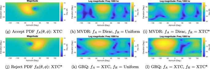

  

  Beampatterns are shown for MVDR / GRQ beamformers designed from a combination of spatial priors for cross-talk cancelation. Dirac and uniform density functions cause over-fitting to the ipsilateral response and under-fitting to the contralateral response respectively unlike the XTC and XTC* priors

  Table 3 Beamformer cross-density probabilistic directivity index (Eq. 35) performance (dB)

• (Dirac, XTC*): MVDR maximizes the response at one ipsilateral ear location ($\theta = \frac {\pi }{3}, \phi = -\frac {\pi }{12}$), minimizes leakage near contralateral ears.

• (XTC, Uniform): GRQ maximizes the responses near ipsilateral ears, minimizes overall leakage.

• (XTC, XTC*): GRQ maximizes the responses and minimizes the leakage near ipsilateral and contralateral ears respectively.

Beamforming PDIs are largest when f_A is the Dirac function; conventional two channel XTC designs set f_R to the Dirac function which places a null at the secondary receiver location to further increase the array cancelation gain but may mismatch if the receiver moves. Setting f_R to the uniform function minimizes the leakage in all directions whereas the XTC* density presents a compromise. For cross-density PDIs, beamforming performance maximally degrades when both f_A,f_R mismatch in the case of (Dirac, Uniform) and (XTC, XTC*). Beamformer GRQ (XTC, XTC*) is 6 dB lower than MVDR (Dirac, Uniform) if receiver locations align with PDI (Dirac, Uniform) conditions. GRQ (XTC, XTC*) is more than 2.5 dB higher than MVDR (Dirac, Uniform) for more realistic PDI (XTC, XTC*) conditions.

We can also evaluate conventional XTC designs under PDI priors. For example, the constant parameter regularized XTC¹ [7] can be generalized for multiple channels in terms of Eq. 35 by setting the accept and reject densities to the dirac delta functions at the accept and reject center angles (θ₁,ϕ₁)∈Ξ₁ and (θ₂,ϕ₂)∈Ξ₂ in Eq. 46 respectively and adding a diagonal loading parameter λ to the rejection covariance matrix:

$$ \begin{aligned} \mathbb{E}_{f_{A}}\left[{\boldsymbol{d} \boldsymbol{d}^{H}}\right] &= \boldsymbol{d}(\theta_{1}, \phi_{1}) \boldsymbol{d}^{T}(\theta_{1}, \phi_{1}), \\ \mathbb{E}_{f_{R}}\left[{\boldsymbol{d} \boldsymbol{d}^{H}}\right] & = \boldsymbol{d}(\theta_{2}, \phi_{2}) \boldsymbol{d}^{T}(\theta_{2}, \phi_{2}) + \lambda \boldsymbol{I}. \end{aligned} $$

(47)

GRQ beamformers that maximize the PDI under Eq. 47 for varying λ are then evaluated w.r.t. the cross-density priors in Table 3 and their expected cancelation gains shown in Fig. 6. The XTC gain at the precise target (θ₁,ϕ₁) and cancelation (θ₂,ϕ₂) angles grows to infinity as λ→0. In practice, we prefer to choose the λ that maximizes a PDI with suitable priors. For example, λ=6.5e−7 maximizes the PDI with (XTC, XTC*) priors at 3 dB expected cancelation gain and sharply declines for larger λ. If the accept region is restricted to the exact target angle in the case of the (Dirac, XTC*) prior, then λ=1.5e−6 maximizes the PDI.

Fig. 6

Constant parameter λ regularized beamformers [7] parameterized by Eq. 47 achieve unbounded XTC gains. Their beampatterns evaluated w.r.t. PDI give the expected XTC gain over different accept and reject density functions

6.3 Beampattern fitting

In applications that require an array to archive a specific beampattern, conventional beamformers such as MVDR and GRQ are ill-suited. The former penalizes a beampattern’s mismatch w.r.t. a target whereas the latter maximizes the expected beampattern’s array gain between two spatial regions. An idealized target beampattern may be specified in some applications such as stereo cross-talk cancelation that places a peak in one region, a null at another, and has sufficient leakage control or side-lobe attenuation everywhere else (see Fig. 3). Given an acoustic simulation of a physical array, we evaluate how close a beamformer can fit to a beampattern.

Far-field anechoic responses belonging to an N=8 channel array on both sides of a wedge (2×4 rectangle array) are simulated at 1 meter distances and then fitted to max truncation-order P=14 SH functions. Two target beampatterns are specified along SH bases of the same max truncation-order using the MoE and PoE models as shown in Fig. 3. The PoE target response has a more directive peak but smoother null than the MoE target. We fit separate beamformer weights to the target beampatterns by minimizing the LS, MLS, and MSLS loss functions from Eqs. 39, 41, and 43 via the OLS, LVE, and the Gauss-Newton methods, respectively. Last, we compare beampatterns by evaluating them across loss functions.

The fitting errors for each set of beamformer weights are shown in Table 4. Rows represent the set of loss function evaluated over beampatterns generated from the optimization method specified in the column. Diagonal entries correspond to the optimizer’s fitting errors and are the minima along each row. Off-diagonal entries correspond to the row’s loss function evaluated on beampatterns produced by other fitting methods where we expect larger errors. Similarity scores in parentheses normalize the errors on each row by dividing by the diagonal entry. Beampatterns generated by MLS and MSLS methods induce large errors and low similarity scores w.r.t. the LS beampattern due to having variable phase responses; MLS and MSLS beampatterns are not unique under arbitrary phase shifts of the beamformer weights. Conversely, LS beampatterns are fitted to both magnitude and phase responses, thereby under-fitting the magnitude and inducing larger MLS and MSLS errors. Last, MLS and MSLS produce beampatterns that are more closely matched in magnitude than their phase; MLS and MSLS generated beampatterns have higher similarity scores than that of LS beampatterns.

Table 4 Beampattern (BP) fitting errors for MoE and PoE targets (similarity scores in parentheses)

The beampatterns visualized in Fig. 7 illustrate the trade-offs made by minimizing each loss function. LS fitted beampatterns that are constrained to match the complex target function over-fits to the 0 radian phase component at the expense of the magnitude component. MLS fitted beampatterns more closely match the target magnitude responses as the phase responses can vary freely. MSLS beampatterns over-fit to regions where the target magnitude response are large due to squaring the magnitude before finding the least squares solution. For the MoE target response, all the beampatterns ignored the sharp null, fitting instead to the wide main lobe. For the PoE target response, the beampatterns fitted both the sharp main lobe and the wide null.

Fig. 7

Beampatterns are shown for far-field beamformers fitted to target MoE and PoE targets specified in Fig. 3 using LS, MLS, and MSLS methods. LS over-fits to a 0 radian phase response. MLS achieves a closer fit to the magnitude target. MSLS over-fits to areas where the magnitude target is large

7 Results and discussion

We derived the SH expansion of Matérn covariance functions of chordal distance over a unit sphere in terms of generalized hypergeometric functions. Simulated anechoic far-field acoustic responses are fitted to RBFs and then transcoded into SH bases, resulting in large data compression. Cross-validation experiments show that the MoE-RBF models have superior bias-variance trade-off compared to direct SH fitting via the TSVD method. Choosing a covariance function with smoothness and locality characteristics that match the spatial acoustic responses improve generalization along unseen areas on the sphere.

Spatial density functions and beampattern targets are then designed using MoE and PoE methods. This enabled conventional beamforming to be reformulated in terms of PDI and probablistic steering vectors sampled from the SH encoded far-field response and spatial density functions respectively. Experiments show how PDI incorporates uncertainty of ear locations in cross-talk cancelation designs and provide a means to evaluate cancelation performance when the priors change. PDI also provides a useful criteria for controlling the amount of diagonal loading in regularized cross-talk cancelation designs.

Beampattern fitting methods such as LS, MLS, and MSLS are at last reformulated along SH bases. For integrated MLS, it remains an open question whether real-valued phase functions can be fitted along SHs due to spatial phase wrapping and discontinuities. For MSLS, we give closed-form gradients and derivatives along the SH bases. Several metrics for comparing beampattern similarity and errors are presented. Experiments demonstrate how effective each method fits a target cross-talk cancelation beampattern from a simulated acoustic array. LS method underfits the magnitude beampattern and should only be used if a flat phase response over the sphere is desirable. MLS equally fits to both peaks and nulls whereas MSLS overfits to peaks in the target beampattern.

8 Conclusions

Data-dependent far-field beamforming requires an efficient representation for synthesizing simulated acoustic data, spatial density priors, and beampattern designs. The SH basis functions are one such representation where data fitting, kernel function expansions, and magnitude function designs can be encoded or transcoded from other methods commonly used in practice. This allows conventional beamforming and beampattern fitting methods to be reformulated in terms of SH bases yielding solutions that are both closed-form and parametric in the spherical coordinates. As a result, we efficiently fitted and stored the acoustic simulations of an array in a continuous and generalizable format. We evaluated beamforming performance under varying use cases via spatial probabilistic priors and beampattern targets. Last, new device geometries, microphone / speaker topologies, and array designs are iterated upon and compared in rapid prototyping offline.

9 Appendix

The generalized hypergeometric function is expressed in terms of the Porchhammer symbol given by

$$ \begin{aligned} F(a, b, z) &= \sum_{k=0}^{\infty} \frac{\prod_{i=1}^{p} (a_{i})_{k}}{\prod_{j=1}^{q} (b_{j})_{k}} \frac{z^{k}}{k!}, \quad (a)_{k} = \frac{\Gamma(a+k) }{\Gamma(a) }, \end{aligned} $$

(48)

where Γ() is the gamma function.

The MSLS residual, Jacobian, Gradient, and Gauss-Newton Hessian are given by

$$ \begin{aligned} r(\boldsymbol{w}) & = \boldsymbol{G}_{A} (\boldsymbol{w} \otimes \boldsymbol{w}^{*}) - \boldsymbol{G}_{B}, \\ \frac{\partial r(\boldsymbol{w})}{\partial\boldsymbol{w}} & = \boldsymbol{G}_{A} (\boldsymbol{I} \otimes \boldsymbol{w}^{*}), \\ \frac{\partial F(\boldsymbol{w})}{\boldsymbol{w}} & = 2 \left({ \frac{\partial r(\boldsymbol{w})}{\partial\boldsymbol{w}} }\right)^{H} r(\boldsymbol{w}), \\ \frac{\partial}{\partial\boldsymbol{w}} \left({ \frac{\partial F(\boldsymbol{w})}{\partial\boldsymbol{w}}}\right) & \approx 2 \left({ \frac{\partial r(\boldsymbol{w})}{\partial\boldsymbol{w}} }\right)^{H} \frac{\partial r(\boldsymbol{w})}{\partial\boldsymbol{w}}. \end{aligned} $$

(49)

9.1 RBF design parameters

The exponential and squared exponential RBFs in Eqs. 15, 18 have FWHM equal to twice the solution of $e^{-\frac {d^{p}(\Theta) }{p \ell ^{p}}} = \frac {1}{2}$ where $d(\Theta) = \pm \ell (p \ln 2)^{\frac {1}{p}}$. The FWHM in terms of Θ radians is given by

$$ \begin{aligned} \textrm{FWHM}_{p}(\ell) = 4 \sin^{-1} \left({ \frac{\ell (p \ln 2)^{\frac{1}{p}} }{2}}\right), \quad \ell \leq \frac{\pi}{(p \ln 2)^{\frac{1}{p}}}. \end{aligned} $$

(50)

The design parameter ℓ for a target response pair T_dB decibels at T_Θ radians is given by

$$ \begin{aligned} \ell_{p}(T_{\Theta}, \, T_{{dB}}) = 2 \sin \left({\frac{T_{\Theta}}{2}}\right) \left({\frac{-20}{p \, T_{{dB}} \ln{10}} }\right)^{\frac{1}{p}}. \end{aligned} $$

(51)

For Matérn ν=3/2, the FWHM and design parameter ℓ are found by reducing the RBF in Eq. 16 into the Lambert W function given by

$$ \begin{aligned} K_{\frac{3}{2}}(w) & = -w e^{w+1}, \quad w = -\left({1 + \frac{\sqrt{3} d}{\ell}}\right), \\ \frac{d}{\ell} &= \frac{W_{-1} \left({-\frac{K_{\frac{3}{2}}(w)}{e}}\right) + 1}{-\sqrt{3}}, \end{aligned} $$

(52)

where W₋₁(z) branch is used to ensure $\frac {d}{\ell } \geq 0$.

$$ \begin{aligned} \textrm{FWHM}_{\nu=\frac{3}{2}}(\ell) & = 4 \sin^{-1} \left({\frac{\ell \left({W_{-1} \left({ \frac{-1}{2e}}\right) + 1}\right)}{-2 \sqrt{3} }}\right), \\ \ell_{\nu = \frac{3}{2}}(T_{\Theta}, \, T_{{dB}}) & = \frac{-2 \sqrt{3} \sin \left({\frac{T_{\Theta}}{2}}\right)}{W_{-1} \left({\frac{-10^{\frac{T_{{dB}}}{20}} }{e}}\right) + 1}. \end{aligned} $$

(53)

For Matérn ν=5/2, the FWHM and design parameter ℓ are found using either bisection or Newton’s method as the RBF in Eq. 17 has a negative first derivative for all positive w given by

$$ \begin{aligned} K_{\frac{5}{2}} (w) & = \left({ \frac{w^{2}}{3} + w + 1}\right) e^{-w}, \quad w = \frac{ \sqrt{5} d }{\ell}, \\ \frac{\partial K_{\frac{5}{2}} (w) }{\partial w} & = \frac{-w(w+1) e^{-w}}{3} < 0, \quad w > 0. \end{aligned} $$

(54)

$$ \begin{aligned} \textrm{FWHM}_{\nu=\frac{5}{2}}(\ell) & = 4 \sin^{-1} \left({\frac{\ell \, \arg{\min}_{w} \left|{ K_{\frac{5}{2}} (w) - \frac{1}{2}}\right|}{2 \sqrt{5}}}\right), \\ \ell_{\nu = \frac{5}{2}}(T_{\Theta}, \, T_{{dB}}) & = \frac{2\sqrt{5} \sin \left({\frac{T_{\Theta}}{2}}\right) }{\arg{\min}_{w} \left|{ K_{\frac{5}{2}} (w) - 10^{\frac{T_{{dB}}}{20}} }\right|}. \end{aligned} $$

(55)

9.2 Error metrics

The NRMSE is computed over N_∗ test samples $\tilde {X}$ and scaled by the full samples X’s standard deviation σ:

$$ \begin{aligned} \textrm{NRMSE} & = \sqrt{\frac{\sum_{i=0}^{N_{*}} \left|{f(\theta_{i}, \phi_{i}) - \tilde{X}_{i}}\right|^{2} }{N_{*} \, \sigma^{2}} }, \\ \sigma^{2} & = \mathbb{E} \left[{\left|{X - \mathbb{E} \left[{X}\right] }\right|^{2}}\right]. \end{aligned} $$

(56)

The NRMSIE between function f(θ,ϕ) and target function $\bar {f}(\theta, \phi)$ over the spherical coordinates reduces to the squared SH residual error and normalized by the target function’s standard deviation:

$$ \begin{aligned} \textrm{NRMSIE} & = \sqrt{\frac{1}{4 \pi \sigma^{2}} \int_{\theta} \int_{\phi} \left|{f(\theta, \phi) - \bar{f}(\theta, \phi) }\right|^{2} \, d \Theta} \\ & \approx \sqrt{\frac{\left({\boldsymbol{C}_{f} - \boldsymbol{C}_{\bar{f}} }\right)^{H} \left({\boldsymbol{C}_{f} - \boldsymbol{C}_{\bar{f}}}\right) }{4 \pi \sigma^{2}}}, \\ \sigma^{2} & = \mathbb{E} \left[{\left|{\bar{f}(\theta, \phi) - \mathbb{E} \left[{\bar{f}(\theta, \phi)}\right] }\right|^{2}}\right] \\ & \approx \frac{\boldsymbol{C}^{H}_{\bar{f}} \boldsymbol{C}_{\bar{f}} - C_{0 \bar{f}}^{0*} C_{0 \bar{f}}^{0} }{4 \pi}. \end{aligned} $$

(57)

References

M. Abramowitz, I. A. Stegun (eds.), Handbook of mathematical functions with formulas, graphs, and mathematical tables. Vol. 55 (US Government printing office, 1972).
J. Ahrens, M. R. P. Thomas, I. Tashev, in Proceedings of The 2012 Asia Pacific Signal and Information Processing Association Annual Summit and Conference, Hollywood, California, USA. HRTF magnitude modeling using a non-regularized least-squares fit of spherical harmonics coefficients on incomplete data, (2012).
J. Ahrens, S. Bilbao, Computation of spherical harmonic representations of source directivity based on the finite-distance signature. IEEE/ACM Trans. Audio Speech Lang. Process.29:, 83–92 (2020).
G. Arfken, “Spherical Harmonics” and “Integrals of the Products of Three Spherical Harmonics.” §12.6 and 12.9 in Mathematical Methods for Physicists, 3rd ed (Academic Press, Orlando, 1985).
A. Chhetri, M. Mansour, W. Kim, G. Pan, in 2019 27th European Signal Processing Conference (EUSIPCO). On acoustic modeling for broadband beamforming (IEEE, 2019), pp. 1–5.
A. Chhetri, et al., in 26th European Signal Processing Conference (EUSIPCO). Multichannel audio front-end for far-field automatic speech recognition (IEEE, 2018).
E. Y. Choueiri, Optimal crosstalk cancellation for binaural audio with two loudspeakers. Vol. 28 (Princeton University, 2008).
COMSOL MultiphysicsⓇ v. 5.6, www.comsol.com (COMSOL AB, Stockholm. https://www.comsol.com/support/knowledgebase/1223.
R. Duraiswami, et al., in IEEE Workshop on Applications of Signal Processing to Audio and Acoustics. Plane-wave decomposition analysis for spherical microphone arrays, (2005).
A. R. Edmonds, Angular Momentum in Quantum Mechanics (Princeton University Press, Princeton, 1957).
M. J. Evans, J. A. S. Angus, A. I. Tew, Analyzing head-related transfer function measurements using surface spherical harmonics. J. Acoust. Soc. Am.104(4), 2400–2411 (1998).
T. Gneiting, Strictly and non-strictly positive definite functions on spheres. Bernoulli. 19(4), 1327–1349 (2013).
J. Guinness, M. Fuentes, Isotropic covariance functions on spheres: Some properties and modeling considerations. J. Multivar. Anal.143:, 143–152 (2016).
P. C. Hansen, The truncated SVD as a method for regularization. BIT Numer. Math.27(4), 534–553 (1987).
R. A. Horn, C. R. Johnson, Matrix Analysis (2nd ed.) (Cambridge University Press, Cambridge, 2012).
C. Huang, H. Zhang, S. M. Robeson, On the validity of commonly used covariance and variogram functions on the sphere. Math. Geosci.43(6), 721–733 (2011).
J. Ivanic, K. Ruedenberg, Rotation matrices for real spherical harmonics. Direct determination by recursion. J. Phys. Chem.100(15), 6342–6347 (1996).
D. P. Jarrett, E. A. P. Habets, P. A. Naylor, in 2010 18th European Signal Processing Conference. 3D source localization in the spherical harmonic domain using a pseudointensity vector, (2010), pp. 442–446.
D. P. Jarrett, E. A. P. Habets, P. A. Naylor, Theory and applications of spherical microphone array processing, vol. 9 (Springer, New York, 2017).
P. W. Kassakian, Convex approximation and optimization with applications in magnitude filter design and radiation pattern synthesis. Diss (University of California, Berkeley, 2006).
Z. Li, R. Duraiswami, Flexible and optimal design of spherical microphone arrays for beamforming. IEEE Trans. Audio Speech Lang. Process.15(2), 702–714 (2007).
Y. Luo, W. Kim, in 2020 28th European Signal Processing Conference (EUSIPCO). Fast Source-Room-Receiver Acoustics Modeling, (2021), pp. 51–55.
J. Mercer, Xvi. functions of positive and negative type, and their connection the theory of integral equations. Philosophical transactions of the royal society of London. Ser. A Containing Pap. Math. Phys. Character. 209(441-458), 415–446 (1909).
C. Müller, Spherical harmonics. Vol. 17 (Springer, 2006).
M. Park, B. Rafaely, Sound-field analysis by plane-wave decomposition using spherical microphone array. J. Acoust. Soc. Am.118(5), 3094–3103 (2005).
A. M. Pasquala, J. R. Arrudaa, P. Herzogb, Optimal array pattern synthesis with desired magnitude response. J. Acoust. Soc. Am.123(5), 3653–3653 (2008).
B. Rafaely, Fundamentals of spherical array processing, Vol. 16 (Springer International Publishing, 2018).
C. E. Rasmussen, C. K. I. Williams, Gaussian processes for machine learning (MIT Press, Cambridge, 2005).
P. N. Samarasinghe, et al., Spherical harmonics based generalized image source method for simulating room acoustics. J. Acoust. Soc. Am.144(3), 1381–1391 (2018).
H. Saruwatari, et al., Blind source separation combining independent component analysis and beamforming. EURASIP J. Adv. Signal Process.11(2003), 1–12 (2003).
I. Schoenberg, Positive definite functions on spheres. Duke Math. J.1:, 172 (1988).
M. L. Stein, Interpolation of Spatial Data: Some Theory for Kriging (Springer Series in Statistics, New York, 1999).
V. Loan, F. Charles, Generalizing the singular value decomposition. SIAM J. Numer. Anal.13(1), 76–83 (1976).
D. B. Ward, G. W. Elko, in Proceedings of the 1998 IEEE International Conference on Acoustics, Speech and Signal Processing, ICASSP ’98 (Cat. No.98CH36181), 6. Optimum loudspeaker spacing for robust crosstalk cancellation, (1998), pp. 3541–3544.
Wolfram Research, Inc., Mathematica, Version 12.3.1 (Wolfram Research, Inc., Champaign, 2021). https://www.wolfram.com/mathematica.
D. N. Zotkin, R. Duraiswami, N. A. Gumerov, in 2009 IEEE Workshop on Applications of Signal Processing to Audio and Acoustics. Regularized HRTF fitting using spherical harmonics, (2009), pp. 257–260.
F. Zotter, et al., A beamformer to play with wall reflections: The icosahedral loudspeaker. Comput. Music J.41(3), 50–68 (2017).
Acknowledgements
We thank the audio technology team at Amazon for providing acoustic simulation data (Jim Sun, Sanjay Yengul) and management (Wontak Kim).
Funding
The work is funded by Amazon.com Inc.
Author information
Authors and Affiliations
Contributions
Authors’ contributions
Yuancheng Luo is the sole author of the work. The author read and approved the final manuscript.
Authors’ information
Yuancheng Luo received his PhD. from the Department of Computer Science at the University of Maryland, College Park in 2014. He is currently a research scientist in the audio hardware-technology team at Amazon Inc.
Corresponding author
Ethics declarations
Competing interests
The authors declare that they have no competing interests.
Additional information
Publisher’s Note
Springer Nature remains neutral with regard to jurisdictional claims in published maps and institutional affiliations.
Rights and permissions
Open Access This article is licensed under a Creative Commons Attribution 4.0 International License, which permits use, sharing, adaptation, distribution and reproduction in any medium or format, as long as you give appropriate credit to the original author(s) and the source, provide a link to the Creative Commons licence, and indicate if changes were made. The images or other third party material in this article are included in the article’s Creative Commons licence, unless indicated otherwise in a credit line to the material. If material is not included in the article’s Creative Commons licence and your intended use is not permitted by statutory regulation or exceeds the permitted use, you will need to obtain permission directly from the copyright holder. To view a copy of this licence, visit http://creativecommons.org/licenses/by/4.0/.
About this article
Cite this article
Luo, Y. Spherical harmonic covariance and magnitude function encodings for beamformer design. J AUDIO SPEECH MUSIC PROC. 2021, 41 (2021). https://doi.org/10.1186/s13636-021-00230-7
Received:
Accepted:
Published:
DOI: https://doi.org/10.1186/s13636-021-00230-7