the Creative Commons Attribution 4.0 License.
the Creative Commons Attribution 4.0 License.
 | 29 Nov 2021
Comparison of inorganic chlorine in the Antarctic and Arctic lowermost stratosphere by separate late winter aircraft measurements
Markus Jesswein
Heiko Bozem
Hans-Christoph Lachnitt
Peter Hoor
Thomas Wagenhäuser
Timo Keber
Tanja Schuck
Andreas Engel
Stratospheric inorganic chlorine (Cly) is predominantly released from long-lived chlorinated source gases and, to a small extent, very short-lived chlorinated substances. Cly includes the reservoir species (HCl and ClONO2) and active chlorine species (i.e., ClOx). The active chlorine species drive catalytic cycles that deplete ozone in the polar winter stratosphere. This work presents calculations of inorganic chlorine (Cly) derived from chlorinated source gas measurements on board the High Altitude and Long Range Research Aircraft (HALO) during the Southern Hemisphere Transport, Dynamic and Chemistry (SouthTRAC) campaign in austral late winter and early spring 2019. Results are compared to Cly in the Northern Hemisphere derived from measurements of the POLSTRACC-GW-LCYCLE-SALSA (PGS) campaign in the Arctic winter of 2015/2016. A scaled correlation was used for PGS data, since not all source gases were measured. Using the SouthTRAC data, Cly from a scaled correlation was compared to directly determined Cly and agreed well. An air mass classification based on in situ N2O measurements allocates the measurements to the vortex, the vortex boundary region, and midlatitudes. Although the Antarctic vortex was weakened in 2019 compared to previous years, Cly reached 1687±19 ppt at 385 K; therefore, up to around 50 % of total chlorine was found in inorganic form inside the Antarctic vortex, whereas only 15 % of total chlorine was found in inorganic form in the southern midlatitudes. In contrast, only 40 % of total chlorine was found in inorganic form in the Arctic vortex during PGS, and roughly 20 % was found in inorganic form in the northern midlatitudes. Differences inside the two vortices reach as much as 540 ppt, with more Cly in the Antarctic vortex in 2019 than in the Arctic vortex in 2016 (at comparable distance to the local tropopause). To our knowledge, this is the first comparison of inorganic chlorine within the Antarctic and Arctic polar vortices. Based on the results of these two campaigns, the differences in Cly inside the two vortices are substantial and larger than the inter-annual variations previously reported for the Antarctic.
- Article
(3415 KB) -
Supplement
(2667 KB) - BibTeX
- EndNote


The Antarctic ozone hole is a recurring event that was first documented by Farman et al. (1985) and has been observed annually since the 1980s. Polar ozone depletion is predominantly driven by anthropogenic chlorine and bromine from long-lived halogenated species (Molina and Rowland, 1974; Engel et al., 2018b). The primary mechanisms for the depletion of ozone (O3) in the polar stratosphere are the catalytic cycles with halogen-containing free radicals as chain carriers (Molina et al., 1987). Chlorine substances involved in rapid ozone depletion are Cl, Cl2, ClO, and ClOOCl and can be summarized as ClOx. Additionally, hydrogen chloride (HCl) and chlorine nitrate (ClONO2) contribute to ozone depletion as they enable the production of active chlorine through heterogeneous reactions on polar stratospheric clouds (PSCs) during polar winter with low temperatures (e.g., Crutzen and Arnold, 1986; Molina et al., 1987; Solomon, 1999). They are therefore called reservoir species. Chemically active chlorine (ClOx) and the reservoir gases together form the total inorganic chlorine (Cly), also called available chlorine. Equivalent effective stratospheric chlorine (EESC) is a simple metric that sums the effect of ozone-depleting substances (ODSs) as an equivalent amount of inorganic chlorine in the stratosphere (Newman et al., 2007; Daniel et al., 1995). Changes to the EESC are mainly due to Cly, as Bry makes up a smaller fraction (Strahan et al., 2014).
The size of the Antarctic ozone hole varies and depends on the amount of Cly and on stratospheric temperature and dynamics (e.g., Newman et al., 2004). However, Cly data are sparse in the polar stratosphere, and there are few measurements of total organic chlorine (CCly) in this area. In contrast, there are many more observations from, e.g., remote sensing instruments of nitrous oxide (N2O), which can be used to determine Cly. A common tool to determine Cly is the usage of scaled correlations. Strahan et al. (2014) used Microwave Limb Sounder (MLS) N2O measurements and a scaled correlation between N2O and Cly from Schauffler et al. (2003) to show that inter-annual variability of Cly for 2004–2012 (−200 to +150 ppt) can be up to 10 times larger than the expected 20–22 ppt yr−1 decline rate due to the Montreal Protocol. Strahan and Douglass (2018) again used MLS measurements of O3, HCl, and N2O to show that Antarctic Cly levels have decreased by 223 ± 93 ppt over a 9-year period (2013–2016 compared to 2003–2007), equivalent to an annual rate of 25 ± 10 ppt yr−1 (∼ 0.8 % yr−1). It is thus important to know whether and how correlations can be transferred from another time period and possibly another region (i.e., the other hemisphere). Due to the phase-out of the long-lived chlorinated species, Cly shows a long-term negative trend (e.g., Newman et al., 2007), whereas N2O exhibits a positive trend (Engel et al., 2018b). This leads to a changing relationship between Cly and N2O with time that must be taken into account. The concept of mean arrival time (Γ*) can be used to normalize correlations of chemically active tracers and scale them to the time of interest (Plumb et al., 1999). The normalized correlations do not change with time and the resulting scaled correlations are used to calculate Cly.
Ozone destruction in the stratosphere is closely linked to the polar vortex. Due to a temperature difference and consequently to a latitudinal pressure gradient between the polar and midlatitude stratosphere (e.g., Schoeberl and Hartmann, 1991), a state with a strong westerly wind in the stratosphere is established (polar night jet). This jet acts as a transport barrier, leading to strong latitudinal gradients of potential vorticity and long-lived substances like N2O (e.g., Hartmann et al., 1989). This isolation of the vortex leads to different concentrations of trace gases within the vortex compared to those in the stratosphere of the midlatitudes. The effect is further enhanced by diabatic descent over the winter, leading to substantially different distributions of trace gases inside and outside the vortex on the same potential temperature (Θ) surface. The polar vortex core can thus be described as a quasi-isolated vessel, separated from the midlatitude stratosphere by the vortex boundary region. In order to differentiate between air masses inside and outside the vortex, a classification of the measurements is needed.
In this study, inorganic chlorine (Cly) was quantified in the Arctic and Antarctic vortex. Calculations of Cly are based only on long-lived chlorinated substances. There is an additional contribution to total stratospheric chlorine from the very short-lived chlorinated substances. Engel et al. (2018b) estimated a contribution of 115(75–169) ppt from very short-lived substances for 2016. Hossaini et al. (2019) estimated a contribution of about 111 ± 22 ppt, of which 13 ± 4.6 ppt are already in inorganic form, which is not considered in this analysis. A new air mass classification system was used for this purpose, based on high-resolution in situ measurements during the campaigns, to map measurements to the vortex, vortex boundary region, and midlatitudes. Results of the Southern Hemisphere Transport, Dynamic and Chemistry (SouthTRAC) campaign from the Antarctic winter and spring 2019 are used to compare Cly of the Southern Hemisphere with Cly of the Northern Hemisphere from measurements of the POLSTRACC-GW-LCYCLE-SALSA (PGS) campaign in the Arctic winter of 2015/2016. An overview of the atypical Antarctic vortex 2019 can be found in Wargan et al. (2020). The evolution of the 2015/2016 Arctic vortex is reported in Manney and Lawrence (2016). Since not all source gases were measured during PGS, a scaled correlation was used and showed the capability of this method as a proxy for sparse data in comparison to the determination from the source gases used for SouthTRAC measurements. Section 2 is a brief introduction to the SouthTRAC campaign and the observations used for this study. Section 3 explains the identification of the vortex, vortex boundary, and midlatitude region. The derivation of inorganic chlorine and the comparison of the methods, the distribution during the late Antarctic winter of 2019, and the comparison of Arctic and Antarctic Cly are all discussed in Sect 4. Section 5 sums up and concludes the findings.
In late winter and early spring of 2019, the Southern Hemisphere Transport, Dynamics, and Chemistry (SouthTRAC) campaign took place to investigate dynamical and chemical composition aspects of the Antarctic upper troposphere and lower stratosphere (UTLS) and gravity waves up to the mesosphere (Rapp et al., 2020). Flights were performed with the German High Altitude and LOng Range Research Aircraft (HALO), which is capable of reaching an altitude of around 14.5 km or 420 K potential temperature. To meet the dynamical and chemical objectives (see https://www.pa.op.dlr.de/southtrac/home/science/scientific-objectives/, last access: 22 November 2021), the aircraft was based in Rio Grande, Argentina (RGA, 53∘ S, 67∘ W). Thus, regions of gravity wave breaking (southern Atlantic and eastern Pacific) and Antarctica were in the range of the aircraft. The campaign was split into two phases. The first phase took place from 6 September to 9 October 2019 to target the dynamical objectives (e.g., Rapp et al., 2020). The second phase took place from 2 to 15 November 2019 to sample polar vortex remnants, as well as perform other tasks. Furthermore, the transfer flights were part of the scientific flights and provide additional information for all objectives.
HALO performed 23 scientific flights with in total 183 hours of measurement time. Nine of these flights were transfer flights from Oberpfaffenhofen (EDMO), Germany, to Rio Grande (RGA), Argentina, and back via Sal (SID), Cabo Verde, and Buenos Aires (EZE), Argentina (see Fig. 1a). Within the first transfer from EDMO to RGA, there was an additional local flight operated from SID. The remaining flights were local flights, with 10 in the first phase and 3 in the second phase. The second phase was terminated early due to technical problems but still provided 27 h of measurements. Thus, it was possible to investigate a region of around 36–70∘ S and 32–84∘ W (see Fig. 1b). The airplane reached a maximum potential temperature of 409 K during the campaign.
The following is a brief explanation of the meteorological data and the instruments and types of measurements used for this work.
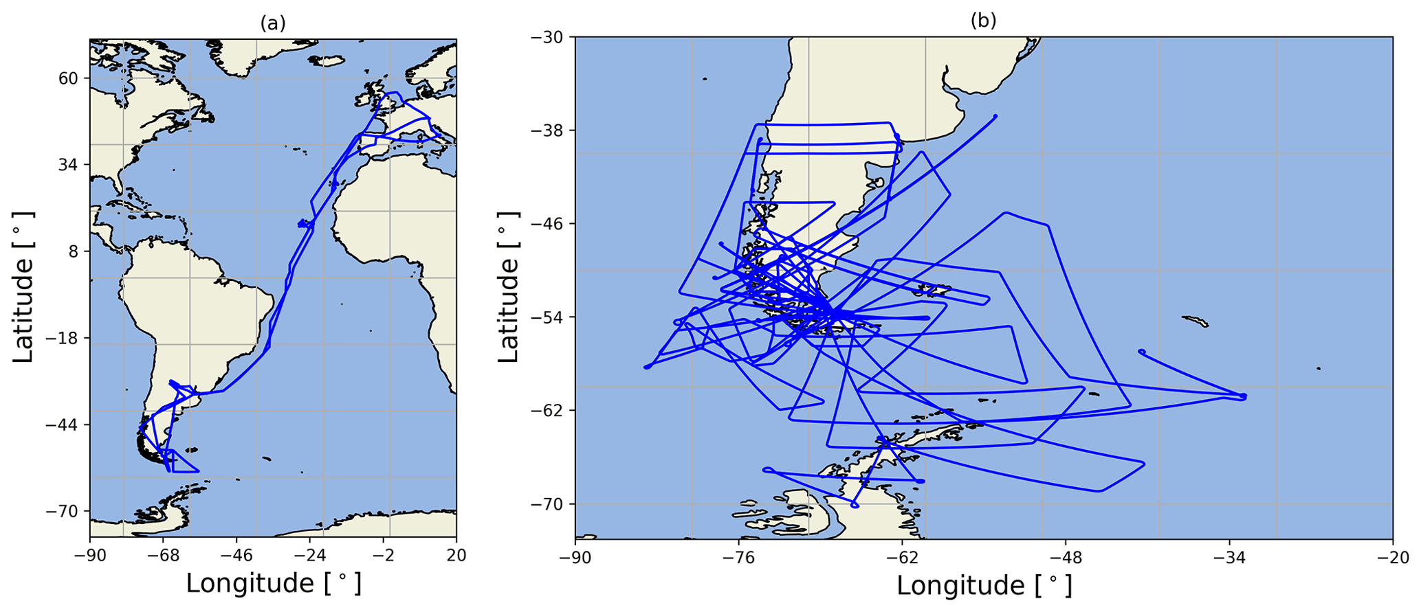
Figure 1Flight tracks of HALO of (a) the transfers from and to Oberpfaffenhofen, Germany (48∘ N, 11∘ E) and (b) during the two phases with the base in Rio Grande, Argentina (53∘ S, 67∘ W).
2.1 Meteorological data
HALO was equipped with a wide range of in situ and remote sensing instruments. In addition to the scientific instruments installed for the measurement campaign, the Basic Halo Measurements and Sensor System (BAHAMAS) is part of HALO. BAHAMAS is installed permanently and provides meteorological and aircraft parameters along the flight trajectory (DLR, 2020).
The local tropopause information along the flight tracks of HALO was created using the Chemical Lagrangian Model of the Stratosphere (CLaMS) (e.g., Grooß et al., 2014). The underlying meteorological data are taken from ECMWF ERA-5 (Hersbach et al., 2020). In this work, the potential vorticity (PV)-based dynamical tropopause is used (e.g., Gettelman et al., 2011), taking 2 PVU (potential vorticity unit) for the dynamical tropopause. Since the PV tropopause is not physically meaningful in the tropics, the potential temperature level of 380 K was taken as the tropopause if the 2 PVU level lies above.
2.2 Halocarbons and SF6
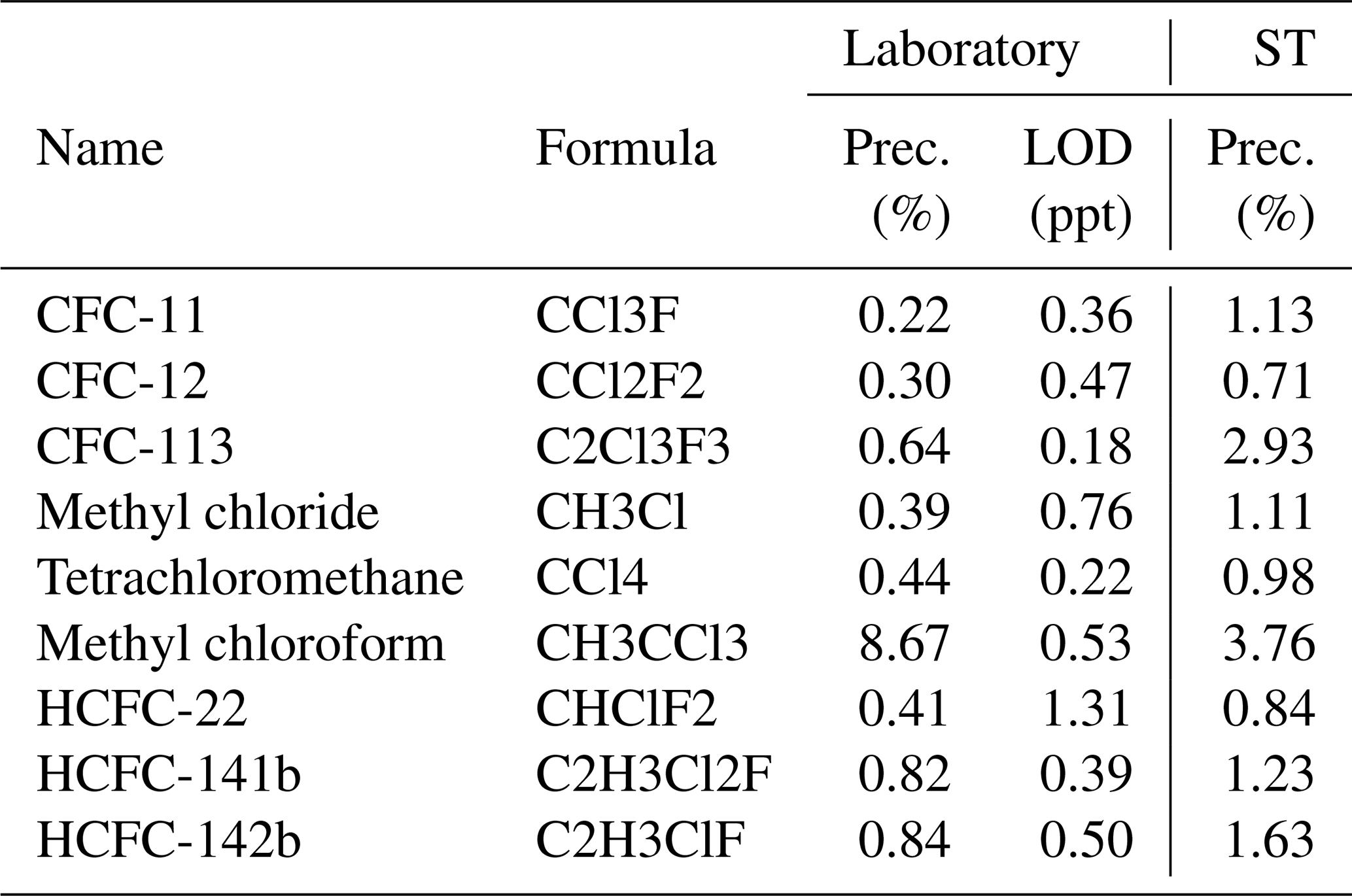
The Gas chromatograph for Observational Studies using Tracers (GhOST) is a two-channel gas chromatographic instrument. The first channel combines an isothermally operated gas chromatograph (GC) with an electron capture detector (ECD) to measure SF6 and CFC-12 at a time resolution of 1 min (hereinafter referred to as GhOST-ECD). A similar setup was used during the SPURT campaign (Bönisch et al., 2009; Engel et al., 2006). The second channel is a combination of temperature programmed GC with a quadrupole mass spectrometer (QP-MS, hereinafter referred to as GhOST-MS). Because of very small mole fractions of the halocarbons, a cryogenic pre-concentration system is installed prior to the GC (Obersteiner et al., 2016; Sala et al., 2014). GhOST was operated successfully during several aircraft campaigns to mainly target brominated halocarbon species, as discussed in Keber et al. (2020). For the SouthTRAC campaign, the ionization mode was changed from negative chemical ionization (NCI) to electron impact ionization (EI) to record full mass spectra. For each substance, one molecular fragment is selected for which the chromatographic peak is not disturbed by other substances. Furthermore, the MS was operated in selected ion monitoring (SIM), scanning pre-selected mass fractions at a preset retention time window. A larger sample volume is needed in EI mode compared to NCI mode. The change of ionization decreased the time resolution from 4 to 6 min per measurement cycle, of which 147 s are needed for sampling air. The performance of the GhOST-MS channel for the chlorinated substances used in this work is shown in Table 1. Displayed are the precisions and detection limits measured shortly before the campaign in the laboratory. Additionally, based on in-flight calibration, precision during the flight can also be calculated. As the conditions in the airplane are more variable than in a laboratory, especially when changing the flight level, this affects the precision of the measurements. The frequency of calibration measurements during a flight is much lower than in the laboratory, making it less stable than the laboratory value. Therefore, precision drops for most of the substances by up to a factor of 4. The exceptions are CFC-11, CFC-113, and methyl chloroform. Methyl chloroform shows a significantly better precision during the campaign, whereas the precision of CFC-12 and CFC-113 measurements was much poorer. It is difficult to determine exactly what the poorer precisions of these two substances can be attributed to. The chromatographic peak of CFC-11 is very narrow, and variable environmental conditions (due to changes in altitude, pressure, and temperature in the cabin) have an influence on the peak shape. The amount of water in the analysis system is also important and is kept as low as possible by drying before pre-concentration. As the chromatographic peak of CFC-113 is close to the chromatographic peak of water, small changes in water can affect the chromatographic peak of CFC-113. CFC-12 and SF6 with the GhOST-ECD channel were measured with a precision of 0.2 % and 0.64 %, respectively. The instrument was tested for nonlinearities and memory effect, and correction was done where necessary (see Sala et al., 2014, for details). Mixing ratios in this work are reported as dry mixing ratios on AGAGE (Advanced Global Atmospheric Gases Experiment) scales.
Table 1Chlorinated species measured with the GhOST-MS. The precisions and limit of detections (LODs) of GhOST were determined in the laboratory shortly before the SouthTRAC (ST) campaign, and mean precision was calculated during the flights.
2.3 N2O
Measurements of N2O were performed with the University of Mainz Airborne Quantum Cascade Laser-spectrometer (UMAQS), which also provided data for CH4, CO, CO2, and OCS during SouthTRAC. The instrument is based on direct absorption spectroscopy using a continuous-wave quantum cascade laser with a sweep rate of 2 kHz (Müller et al., 2015). During SouthTRAC the instrument was calibrated in situ against two standards of different concentrations, which are compared against primary standards (NOAA) prior to and after campaign phases.
Under typical flight conditions at flight level, N2O was measured with an overall uncertainty of 0.6 ppb relative to the calibration standards. The noise of the 1 Hz data was 0.1 ppb (1σ). Note that this is an upper limit since the data are corrected post-flight for drift effects based on the in-flight calibrations.
Chlorine activation tends to occur in the coldest regions of the stratosphere and is therefore typically co-located with the polar vortex. Furthermore, as the polar night jet acts as a barrier, air composition is different inside and outside the vortex. High concentrations of reactive halogenated substances can be maintained inside the vortex because there is little mixing with the surrounding area. During the HALO flights, the aircraft encountered air masses with different characteristics due to their origin. To make systematic conclusions about the distribution of trace gases, a reliable, accurate method of separating the measurements in terms of their region of origin is needed. For this reason, the following describes how air masses have been classified using highly resolved in situ measurements.
3.1 Air mass classification by in situ measurements
The maximum gradient of PV is a commonly used indicator to define the location of the vortex edge, also known as the Nash criterion (Nash et al., 1996). PV is a model-derived quantity. Although the underlying meteorological reanalyses have a fairly high resolution these days (e.g., Hersbach et al., 2020), small-scale features like vortex filaments with different chemical compositions may not be well resolved. In this work, an extended version of the vortex definition by Greenblatt et al. (2002) is used instead. The technique by Greenblatt et al. (2002) uses the tight correlation between N2O and potential temperature to determine the inner edge of the vortex boundary. N2O can be measured in situ with a high time resolution to reveal small-scale structures in the atmosphere. As already mentioned in Sect. 1, air inside the polar vortex has a substantially different composition regarding trace gases than air outside the vortex. A tracer like N2O exhibits a horizontal gradient across the vortex edge in the stratosphere with lower mixing ratios inside the vortex and higher mixing ratios outside the vortex. In addition, N2O has small variability inside the vortex on constant isentropic surfaces (variability of about 6 ppb Greenblatt et al., 2002). This is an indication of well-mixed air inside the polar vortex due to the long isolation in polar winter. The vertical profile of N2O in the midlatitudes shows a weak gradient but a high variability as it is influenced by both tropical and polar air (Krause et al., 2018; Marsing et al., 2019). In between there is a transition region (vortex boundary region), which is influenced by the vortex as well as by midlatitudes. Towards tropopause altitudes, the transport barrier of the polar vortex disappears and a classification is not possible.
Based on the method of Greenblatt et al. (2002), one flight is chosen to generate a vortex reference profile. This flight should ideally be completely in the vortex. However, during the SouthTRAC campaign there was no flight that only sampled vortex air. In addition, there is an interest in not only distinguishing between vortex and non-vortex air, but also in assigning the campaign measurements to the vortex, vortex boundary region, and midlatitudes. For this reason, several flights were used to create reference profiles for the vortex and midlatitudes. The composition of the lowermost stratosphere is affected by diabatic descent inside and outside the polar vortex and quasi-isentropic mixing with air from lower latitudes. In addition, mixing at the extratropical tropopause affects the lowest 20–25 K above the local tropopause (Hoor et al., 2004, 2005). Therefore, classification was done with two vertical coordinates, potential temperature (Θ) and potential temperature above the local tropopause (ΔΘ).
The vortex reference profile (see Fig. 2) was generated from all flights that are assumed to contain measurements within vortex air. Data from these flights were pre-filtered by taking only the measurements polewards of 60∘ S equivalent latitude (Butchart and Remsberg, 1986) and 20 K above the local tropopause. With an iterative filter procedure (see Appendix A) the lower envelope of the remaining measurements is obtained and is used to generate the vortex profile function (Werner et al., 2010). For the midlatitude profile (see Fig. 2), all flights were taken into account, focusing only on measurements between 40 and 60∘ S equivalent latitude and again 20 K above the local tropopause. This time, the upper envelope of the measurements was evaluated by the iteration procedure to build a reference profile function for the midlatitudes. As an intermediate step to the final profiles, the measurements of the lower and upper envelope are binned in 5 K intervals of Θ or ΔΘ (see Fig. S2c and d). Mean values of the binned profiles are then used to generate a polynomial fit function for the vortex profile and the midlatitude profile (Fig. S3). The two reference profiles in Θ coordinates are displayed in Fig. 2a, and the two reference profiles in ΔΘ coordinates are displayed in Fig. 2b.
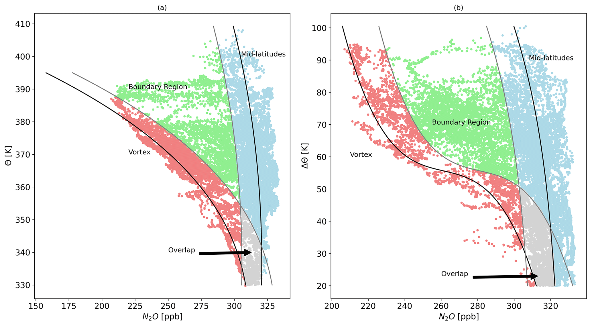
Figure 2Midlatitude and vortex profiles (black) of N2O versus (a) potential temperature (Θ) and (b) potential temperature difference (ΔΘ) from the local PV tropopause. The vortex cutoff criterion (see main text for details) of 20 ppb is illustrated by the grey profile on the right side of the vortex profile. Midlatitude variability of 15 ppb is illustrated with the grey profile on the left side of the midlatitude profile. In between these is the vortex boundary region. The overlap region is declared for the area where the vortex cutoff and midlatitude variability cross. Additionally, N2O measurements classified to the respective region are displayed. Vortex measurements are in red, vortex boundary region measurements are in green, midlatitude measurements are in blue, and overlapping measurements are in grey.
In general, it cannot be assumed that a single N2O vortex profile can be representative for the entire winter. Subsidence of the vortex air by several kilometers due to radiative cooling (Schoeberl and Hartmann, 1991) leads to a changing N2O profile throughout the polar winter. In the lower stratosphere of the Southern Hemisphere, descent generally stops around mid-October (Manney et al., 1994). However, N2O data of the SouthTRAC flights did not reveal strong diabatic descent during the time of the campaign (below Θ=400 K). Therefore, only one reference vortex profile was generated for the campaign.
A vortex and midlatitude reference N2O data set (N2Ovor and N2Omid) can be calculated from Θ or ΔΘ by using the fit function for the vortex and midlatitude profiles for every measurement point of the UMAQS instrument for all flights. The following then applies for each N2O measurement: if the mixing ratio is below the respective N2Ovor plus the prescribed vortex cutoff, then it is assigned to the vortex. Otherwise, if the mixing ratio is above the respective N2Omid minus the associated variability, then it is assigned to the midlatitudes. Mixing ratios above the respective N2Ovor plus the prescribed vortex cutoff and below the respective N2Omid minus the associated variability are assigned to the boundary region. Measurements for which the respective N2Ovor plus the prescribed vortex cutoff and the N2Omid minus the associated variability overlap cannot be uniquely classified and are assigned to both the vortex and the midlatitudes in later analysis. For the prescribed vortex cutoff, the value of 20 ppb proposed by Greenblatt et al. (2002) was used. The associated variability of the midlatitude profile was set to 15 ppb, as the variability in N2O in the midlatitudes is roughly 10 % (Strahan et al., 1999).
3.2 Overview of the sample regions
In 2019, extraordinary meteorological conditions led to a sudden rise in stratospheric temperatures over Antarctica. This minor sudden stratospheric warming (minor SSW) event affected the shape, location, and strength of the polar vortex. From mid-August to early September 2019, the polar vortex was displaced and weakened towards the eastern South Pacific and South America (Safieddine et al., 2020; Wargan et al., 2020). The SouthTRAC campaign flights took place from early September to early October and in the first half of November; thus, they took place shortly after the minor SSW event and captured the late winter evolution of the Antarctic polar vortex.
Figure 3 displays an overview of air mass classification of the local flights of the SouthTRAC campaign (classification in Θ coordinates). Measurements below 20 K of ΔΘ are not classified and are not taken into account here. There are no N2O measurements available from flight ST08 on 11 September, and thus no classification was possible. Vortex air sampling varies from flight to flight depending on the objective of each flight. The vortex and boundary regions were sampled in both phases of the campaign. The first phase includes some flights that predominantly sampled the vortex or vortex boundary region (e.g., flight ST15 on 29 September or flight ST16 on 30 September). In general, vortex air represents about 23 % of flight time in the stratosphere and vortex boundary air about 14 %. More than half (56 %) of the flight time in the stratosphere was in midlatitude air. The use of the ΔΘ coordinates for the air mass classification leads to similar percentage division (not shown here).
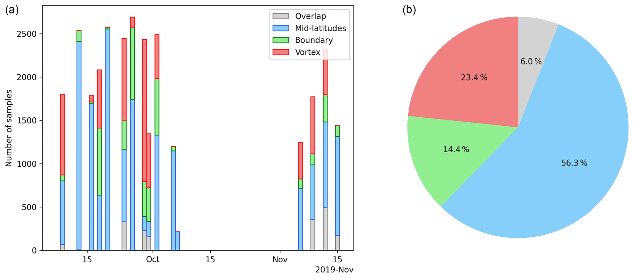
Figure 3Air sampling statistics of the SouthTRAC campaign. (a) The number of classified measurements. Each column represents a single scientific flight. Stacked bars indicate vortex (red), vortex boundary (green), midlatitudes (blue), and undefined (grey) amounts. (b) Percentage of each region in the total of all measurements in the scope of the classification (above ΔΘ of 20 K).
4.1 Up-sampling GhOST-MS measurements
The GhOST-MS measurements have a time resolution of 6 min of which the enrichment and therefore the sampling of air takes around 147 s. With a maximum cruising speed of around 258 m/s, this means that air is sampled along a distance of approximately 38 km per measurement during enrichment. This could lead to a rather coarse resolution where fine structures like filaments and small-scale dynamical perturbations are sometimes not well resolved.
Measuring CFC-12 in both the ECD and MS channels of the instrument allows the measurements of the organic source gases to be up-sampled by using the better-resolved measurements of CFC-12 from the ECD channel. Measurements of CFC-12 in the ECD channel not only have a higher time resolution of 1 min, but they also have better precision than data from the MS channel. As shown in Fig. 4, the correlation between CFC-12 measurements of the two channels for all flights is linear over the whole range of mixing ratios, with a coefficient of determination of R2 = 0.968. Firstly, for each organic source gas, a linear or polynomial fit function is calculated based on the correlation with CFC-12 measurements in the GhOST-MS channel for all flights (correlations contained in the supporting information). Secondly, these fit functions are then used together with the CFC-12 measurements of the ECD channel to calculate the up-sampled mixing ratios of the organic source gases. Flight ST14 from 26 September in Fig. 5 is an example to demonstrate the benefits of the up-sampling. Displayed are the original measurements of CFC-11 of the MS channel as well as the up-sampled CFC-11 values. The background colors indicate to which region the samples can be assigned (classification in Θ coordinates), as described in Sect. 3. The up-sampled values show higher variability and follow the classification well by region. Especially with the sharp gradients, e.g., at 04:10 and 05:50 UTC in Fig. 5, the original lower-resolution data did not capture the transitions well between the regimes compared to the up-sampled data. In the following, the up-sampled data are used for further evaluation.
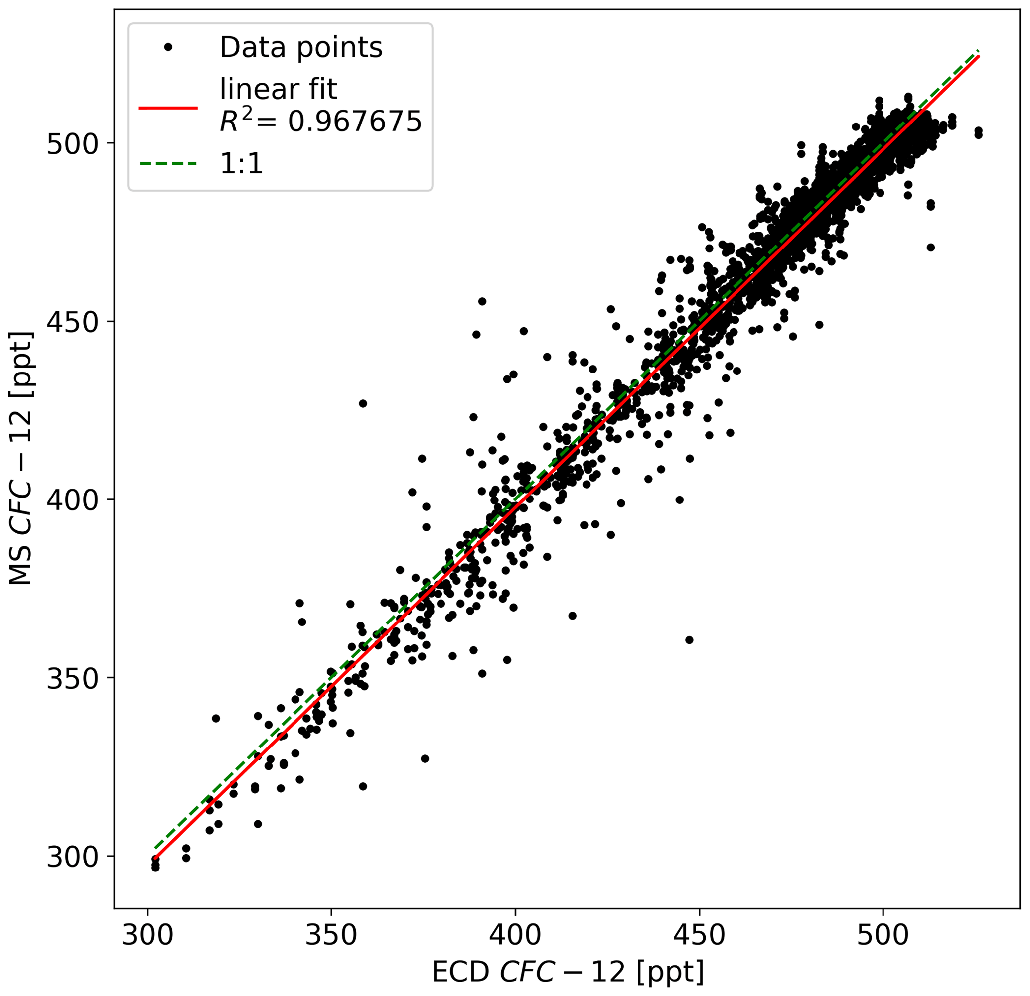
Figure 4Correlation between CFC-12 measured in the GhOST-MS channel and in the GhOST-ECD channel.

Figure 5CFC-11 measured in the GhOST-MS during flight ST14 on 26 September 2019. Original data are shown in red, and measurements up-sampled using CFC-12 from the ECD channel are shown in black. Background colors indicate in which region the samples were taken using the air mass classification in Θ coordinates.
4.2 Semi-direct and indirect calculation of inorganic chlorine
Organic chlorine (CCly) can be calculated directly from the up-sampled GhOST-MS measurements. Thus, Cly can be calculated from Eq. (1) if the mixing ratios of the major chlorine-containing substances at the stratospheric entry point (Cltotal) are known.
Air enters the stratosphere predominantly through the tropical tropopause layer (TTL). During transport into and within the stratosphere, an air parcel exhibits irreversible mixing and cannot be regarded as conserved (Hall and Plumb, 1994). Instead, an air parcel in the stratosphere consists of a multitude of components with different transit times, representing their travel times since they entered the stratosphere. The distribution of the transit times is called the age spectrum G, and the first moment is the mean age Γ (Hall and Plumb, 1994). The concept of the age spectrum can be used to determine mean age values based on observations of chemically inert tracers in the stratosphere. For this purpose, in addition to the age spectrum, tropospheric time series of the inert tracers are required (Engel et al., 2002). This was done for the SouthTRAC campaign by using SF6 measurements of the GhOST-ECD and tropospheric time trends taken from the AGAGE (Advanced Global Atmospheric Gases Experiment) Network (Prinn et al., 2018). Since only the mean age is given, a width parameterization is used to derive the age spectrum by using the ratio of moments (). Hauck et al. (2019) showed that the ratio of moments undergoes seasonal variability and is probably much larger than previously implemented values (e.g., Engel et al., 2002; 0.7 years). A ratio of moments of 1.25 years is chosen here. The age spectrum, together with the tropospheric time trend of the substances of interest, can be used to calculate the stratospheric mixing ratio that would be present without chemical degradation, which thus represents the entry mixing ratio. In the following, Cly derived from the difference between the estimated entry mixing ratios and observed CCly from the in situ measurements (see Eq. 1) is referred to as the semi-direct calculation of Cly.
For the case where measurements of all major chlorine-containing substances are not available, Cly has in the past been calculated indirectly based on correlations derived from previous measurement campaigns. This also applies to Cly from the Northern Hemisphere used later in this paper (see Sect. 4.4). For instance Wetzel et al. (2015) and Marsing et al. (2019) used Cly based on a correlation derived from two balloon flights inside the Arctic polar vortex in 2009 and 2011 from a cryogenic whole-air sampler (Engel et al., 2002). In order to account for tropospheric trends, the correlations between CFC-12 and the other long-lived substances were adapted with a modified method described in Plumb et al. (1999) using the mean arrival time Γ* to derive a correlation function valid for the respective time when the correlation is applied. Plumb et al. (1999) showed that the age spectrum of an inert tracer is not well suited to describe the propagation of chemically active tracers into and through the stratosphere. They introduced a modified age spectrum, called the normalized arrival time distribution G*, which combines chemical loss and transport. The mean arrival time Γ* represents the first moment of this distribution. The mean arrival time Γ* for all the relevant chlorine substances can be parameterized in terms of stratospheric lifetime τ and mean age Γ (Plumb et al., 1999). Using G* instead of G and therefore Γ* instead of Γ is better suited for chemically active tracers because the tail of the transit time distribution is less weighted, especially for substances with shorter stratospheric lifetimes (Engel et al., 2018a; Ostermöller et al., 2017). To transfer the correlations from the balloon observations in 2009 and 2011 to the measurements during SouthTRAC in 2019, the observed mixing ratios are first divided by the respective estimated entry values to derive the normalized mixing ratios. The entry values are calculated by the modified age spectrum and tropospheric time trends from the AGAGE Network for the time of the balloon measurements. Multiplying the normalized mixing ratios by the entry mixing ratio for the time during SouthTRAC then allows a comparison to the directly determined correlations during SouthTRAC. Here, we compare the directly observed correlation from SouthTRAC to the indirectly determined correlations based on previous balloon observations transferred to 2019. Note that the indirectly determined values are based on observations that were not only performed about 10 years earlier but that were also from the Northern Hemisphere instead of the Southern Hemisphere. Figure 6 displays scaled correlations from the balloon observations (red) and correlations from the SouthTRAC data (black) of three long-lived substances against CFC-12. The balloon-based correlations correspond well to the correlations measured during the SouthTRAC campaign. Thus, the balloon-based correlations can be used to determine CCly from CFC-12 alone. As already mentioned earlier, Cltotal is also needed for the calculation of Cly (see Eq. 1). The mean age values derived for the balloon measurements are used for this purpose, and Cltotal is calculated for the conditions during SouthTRAC. Cly is then derived as the difference between Cltotal and CCly.
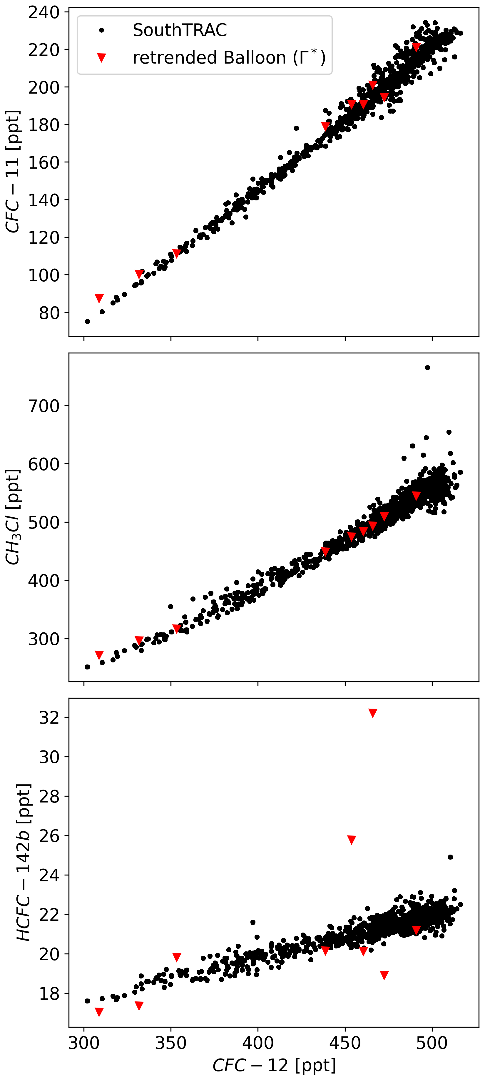
Figure 6Correlation between CFC-12 and CFC-11, between CFC-12 and CH3Cl, and between CFC-12 and HCFC-142b. The raw measurements by GhOST-MS are shown in black, and the balloon observations scaled to the time of the SouthTRAC campaign using mean arrival time are shown in red.
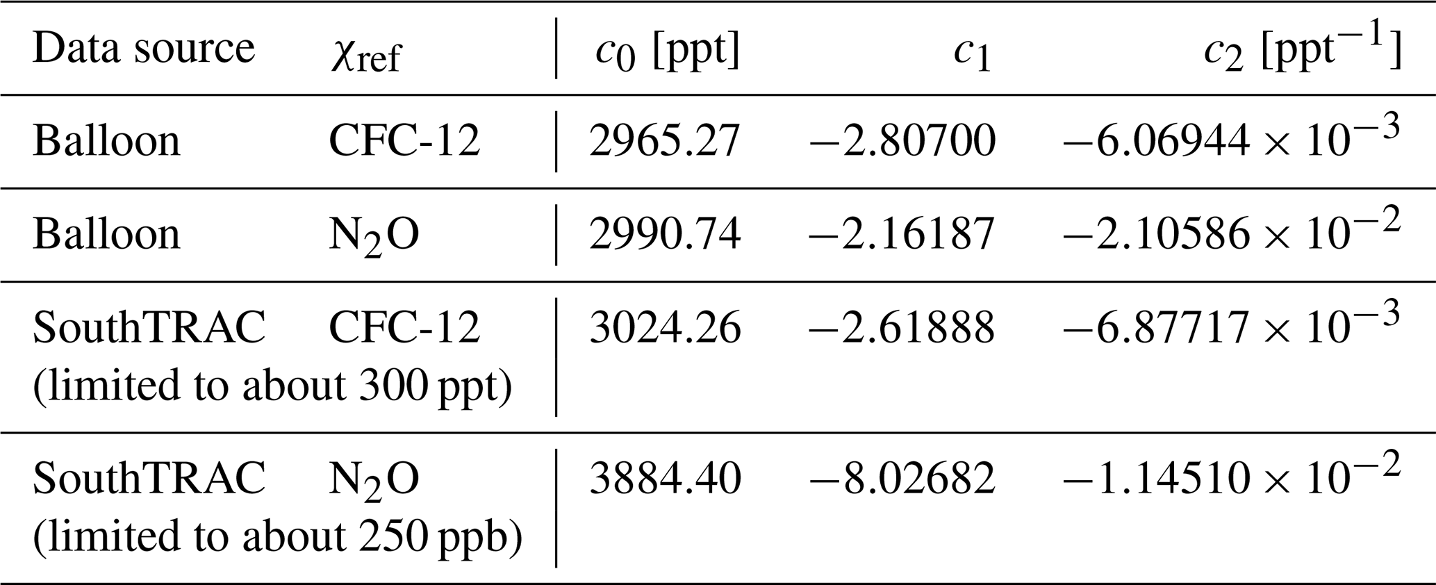
With the good agreement between observed correlations and scaled correlations from the balloon measurements and the previously described determination of Cly, we explore whether Cly can be successfully estimated from CFC-12 alone. Therefore, a correlation function for the conditions during Antarctic late winter 2019 has then been derived for the indirect calculation of Cly as a function of CFC-12 mixing ratios (Eq. 2). The coefficients for the correlation function with CFC-12 as the reference substance based on the balloon measurements can be taken from Table 2. In addition, the fit coefficients are given if one wants to use N2O as the reference. N2O shows a compact correlation with long-lived chlorinated substances and has been used in many publications for the determination of Cly (e.g., Schauffler et al., 2003; Strahan et al., 2014; Strahan and Douglass, 2018). Using CFC-12 from the GhOST-ECD channel and N2O from the UMAQS instrument, we obtain comparable values for Cly (see Fig. S7 in the supporting information). In the following, CFC-12 from the GhOST-ECD channel is used as the reference in Eq. (2) for the indirect determination of inorganic chlorine.
Figure 7 shows semi-directly and indirectly determined inorganic chlorine as a function of mean age. Cly values were binned in intervals of 0.2 years, and the mean values are displayed. For both methods, inorganic chlorine increases with mean age of air as more molecules of the organic source gases are converted to the inorganic form. The difference between the two methods is rather small, with less than around 30 ppt difference between 1 and 4 years of mean age and a maximum difference of about 65 ppt at 5 years of mean age. Recent research suggests that SF6-based mean age is biased because its suggested lifetime has been overestimated (e.g., Ray et al., 2017). As a guideline, Fig. 7 additionally shows a corrected mean age of air using one of the linear fit functions from Leedham Elvidge et al. (2018), based on a comparison of SF6-based mean age with a combined mean age based on five alternative age tracers. The fundamental picture does not change, however, and thus we use the uncorrected mean age of air. The small deviation over the entire range of mean age indicates that adapted correlations from previous measurement campaigns and also from the Northern Hemisphere lead to comparable values in inorganic chlorine determined for the Southern Hemisphere. Hence the metric can be used for the calculations of Cly in the case where only measurements of CFC-12 are available. Since it was possible during SouthTRAC to measure the organic source gases, the Cly determined semi-directly from the measurements was used for further evaluation. However, the good comparability of the two methods offers the possibility to compare Cly from different measurement campaigns, which differ regarding the number of measured chlorinated substances (see Sect. 4.4). With the semi-directly determined Cly during SouthTRAC, correlation functions can be determined. Table 2 contains the coefficients for the correlation functions based on CFC-12 and N2O as references. The correlation functions are limited to the minimum mixing ratio of the respective reference substance taken during the SouthTRAC campaign.
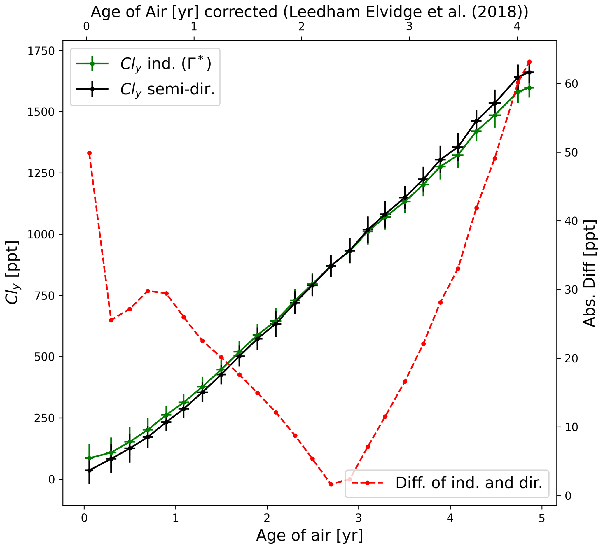
Figure 7Indirectly (green) determined Cly based on balloon observations in 2009 and 2011 and semi-directly (black) determined Cly as a function of age of air (bottom axis) and corrected age of air (top) using a linear fit from Leedham Elvidge et al. (2018). The absolute difference between these methods is shown in red.
Table 2Coefficients of the correlation function to indirectly derive Cly with the respective reference substance for the time of the SouthTRAC campaign (2019.75). Calculation of Cly with CFC-12 or N2O and coefficients based on the balloon observations in 2009 and 2011 (Balloon) and coefficients based on the SouthTRAC measurements (SouthTRAC).
4.3 Chlorine partitioning in the Antarctic winter 2019 lower stratosphere
Since inorganic chlorine plays a major role in ozone depletion, it is worth investigating its distribution in the Antarctic stratosphere. For the analysis only measurements polewards of 40∘ equivalent latitude are used. As a vertical coordinate Θ was chosen. All measurements have been binned into 5 K potential temperature bins between 270 and 420 K (see Fig. 8). Bins that contain fewer than five data points are not included in the analysis. The uncertainties represented by the error bars are the 1σ standard deviations of the means. Up to the potential temperature at which air mass classification begins, the Cly is estimated based on all measurements. From the potential temperature at which air mass classification begins, Cly is estimated separately in each region. Measurements within the overlap area in the classification (see Fig. 2) are counted both as vortex and midlatitude measurements.
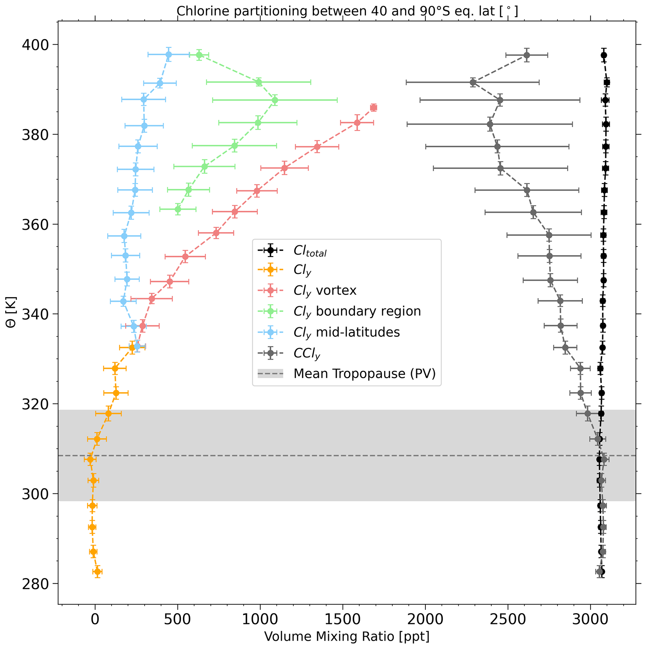
Figure 8Vertical profiles of Cly, Cly by region from 20 K above the local tropopause, CCly, and Cltotal averaged over 40–90∘ S equivalent latitude for all flights during SouthTRAC. The data are displayed as a function of potential temperature. Vertical and horizontal error bars denote 1σ variability. The dashed line shows the averaged PV-based dynamical tropopause with the 1σ variability as a shaded area.
In Fig. 8, the inferred Cly throughout the troposphere is close to zero and increases in the tropopause region. The tropospheric measurements during SouthTRAC are thus consistent with Cltotal derived from ground-based AGAGE measurements. The vertical profiles of vortex, vortex boundary, and midlatitude declared measurements show different gradients. In the midlatitudes, the inorganic chlorine hardly increases between 330 and 380 K, with values between 171±78 and 260±117 ppt, whereas the increase is stronger between 380 and 400 K, reaching a value of 446±124 ppt. The profile of the vortex boundary region increases in the range from 502±110 up to 1090±377 ppt in the Θ interval of 360 to 395 K. The variability of the vortex boundary profile increases with height. This is partly due to the air mass classification, since the range of values in the vortex boundary region increases with increasing potential temperature (see Fig. 2). Inorganic chlorine within the vortex could be obtained from Θ between 330 to 385 K. Cly inside the vortex increases significantly up to a value of 1687±19 ppt. Thus, in late winter and early spring at the highest measured potential temperatures, about half of the recorded chlorine is found in inorganic form. Despite this amount of inorganic chlorine in the lower stratosphere, the total polar ozone column was higher than usual in September 2019. As a result of the minor SSW event, chlorine deactivation began earlier in 2019, and the ozone hole was about 10×106 km2 in size and thus only 20 % of that in mid-September 2018 (Wargan et al., 2020).
4.4 Comparison of Cly in the Antarctic (SouthTRAC) and Arctic (PGS) polar winter
To compare Cly in the Antarctic polar vortex and in the Arctic polar vortex, measurements performed on the HALO aircraft during the PGS campaign were used. PGS consisted of the three partial missions POLSTRACC (Polar Stratosphere in a Changing Climate), GW-LCYCLE (Investigation of the Life cycle of gravity waves), and SALSA (Seasonality of Air mass transport and origin in the Lowermost Stratosphere) to probe stratospheric air during the Arctic winter in 2015/2016 (Oelhaf et al., 2019). Flights of the PGS campaign were conducted from 17 December 2015 until 18 March 2016 and can be separated into two main phases. For this study, only the flights from the second main phase from 26 February to 18 March are investigated, since they took place in a comparable period (later winter). The separation into vortex, vortex boundary, and midlatitude measurements is based on the above-mentioned method using N2O measurements performed by the TRIHOP instrument on board HALO during PGS (Krause et al., 2018) (see Fig. S6 in the Supplement). In Sect. 4.2, the indirect method for the determination of Cly, where a direct measurement of all relevant chlorinated substances is not possible, was shown to provide values comparable to those obtained by the semi-direct method. During PGS, CFC-12 was measured with the ECD channel, but the MS channel was in NCI mode and could not measure all chlorinated substances. Cly was therefore calculated using the indirect method and CFC-12 measurements from the GhOST-ECD channel during PGS. As for SouthTRAC, the scaled correlations from observations of the cryogenic whole-air sampling on two balloon flights inside the Arctic polar vortex in 2009 and 2011 were used (correlation function for the Arctic winter 2015/2016 can be taken from the Supplement).
Figure 9 displays the mean vertical profiles of Cly inside the vortex and Cltotal of the respective hemisphere. Measurements from the individual campaigns have been binned into 5 K potential temperature (a) and potential temperature difference to the local tropopause (b). The PV-based dynamical tropopause was used for PGS, as was done for the SouthTRAC analysis. The mean PV-based tropopause was at 306 K during PGS, only slightly lower than that during SouthTRAC at 308 K. Independent of the vertical coordinate, total chlorine (Cltotal) in the lower stratosphere decreased from the time of PGS (2015/2016) to the time of SouthTRAC (2019). The difference between Cltotal from controlled substances during PGS and that during SouthTRAC is about 60±9.6 ppt. This difference can be explained by a combination of temporal trends of controlled substances and interhemispheric gradients. Using the rate of decline from Engel et al. (2018b) of ppt yr−1 for the controlled substances, a difference of about 45 ppt is expected due to the time difference between the two campaigns. The remaining difference of about 15 ppt can be explained by the higher Cltotal in the Northern Hemisphere.

Figure 9(a) Comparison of the vertical profiles of Cly inside the respective vortex where classification was possible and total chlorine from PGS (black) and SouthTRAC (green). Data are averaged over 40 to 90∘ equivalent latitude of the respective hemisphere and are displayed as a function of potential temperature. Vertical and horizontal error bars denote 1σ variability. PV tropopause for PGS (black) and SouthTRAC (green) are displayed as dashed horizontal lines with the 1σ variability as shaded areas. Panel (b) is the same data as (a) but as a function of potential temperature relative to the local tropopause (PV) displayed with a dashed grey line.
Using Θ as the vertical coordinate (Fig. 9a), vertical profiles of vortex classified Cly of PGS and SouthTRAC show different results. Although the Cly vortex profiles are similar until around 350 K, the SouthTRAC profile increased more steeply, reaching values more than 444 ppt larger than those during PGS at the same potential temperatures. Differences are slightly larger when using ΔΘ as the vertical coordinate (Fig. 9b). Although the two Cly profiles lie close together between 20 and 50 K ΔΘ, the differences between them increase to 540 ppt at 65 K ΔΘ. The fraction of total chlorine in the form of Cly during PGS at the same distance from the local tropopause as the maximum SouthTRAC Cly fraction is about 20 % in the midlatitudes (not shown) and about 40 % inside the vortex (Fig. 9b).

Figure 10Difference of the latitude–altitude cross section of Cly from PGS and SouthTRAC. Data are binned using equivalent latitude* and ΔΘ.
Figure 10 shows the difference between PGS and SouthTRAC Cly in a latitude–altitude cross section. Equivalent latitude* was used as a horizontal coordinate, i.e., the geographic latitude for all tropospheric observations and equivalent latitude for all stratospheric ones (Keber et al., 2020); ΔΘ was used as a vertical coordinate. Since the tropopause height of the two hemispheres is different and changes with the season, the tropopause relative coordinate ΔΘ accounts for tropopause variability and allows for better comparison of Cly. The data have been binned in 5∘ latitude and 5 K of potential temperature relative to the local tropopause. Only bins which contain at least five data points were considered in this analysis. The difference was calculated by subtracting each Southern Hemispheric latitude–altitude bin from the equivalent Northern Hemispheric latitude–altitude bin. Values in the troposphere differ only slightly. In the lower stratosphere, a separation into two areas can be seen. In the lower stratosphere at higher latitudes, overall higher mixing ratios were derived during SouthTRAC in comparison to PGS. There are two bins with substantially higher values during SouthTRAC, with around 900 ppt more Cly between 80 and 90 K of ΔΘ and 65 to 70∘ equivalent latitude. This difference is much larger than the difference when comparing vortex classified measurements (Fig. 9). Thus, it is very likely that vortex core and vortex edge values are compared due to the different Arctic and Antarctic vortex size, stability, and strength of the transport barrier. Therefore, performing the comparison in equivalent latitude and potential temperature coordinates removes only some of the sources of discrepancy. The stratosphere of the midlatitudes shows consistently higher Cly values during PGS. The highest values of Cly reached are 315 ppt higher during PGS between 65 and 70 K of ΔΘ and 40 to 45∘ equivalent latitude. The already-mentioned difference of Cltotal between PGS and SouthTRAC amounts to 60±9.6 ppt. This maximum difference of 60±9.6 ppt will only propagate completely to Cly when all chlorine is converted to the inorganic form. Taking into account the difference in Cltotal between the two campaigns would reduce the observed differences in the midlatitudes, where mixing ratios of Cly were higher during PGS, but would increase the differences in the high latitudes, where higher Cly was derived for SouthTRAC. The observed differences in Cly are thus clearly larger than can be explained by the temporal difference in Cltotal. Possible reasons for the observed differences can be derived from the hemispheric difference of the Brewer–Dobson circulation using the age of air as a common metric for transport. Konopka et al. (2015) showed that the age of air is always younger north of 60∘ N than south of 60∘ S in the corresponding season. Older air will be higher in Cly as a larger fraction of total chlorine has already been converted to the inorganic form. Therefore, the observed differences in Cly, with higher Cly values in the southern high latitudes than in the northern high latitudes (see Figs. 9 and 10), are consistent with the differences in the age of air found by Konopka et al. (2015). In addition, Engel et al. (2018b) updated the long-term total column HCl and ClONO2 (representing Cly) record reported by Mahieu et al. (2014) in the stratosphere at Jungfraujoch (46.5∘ N) and at Lauder (45∘ S) through the end of 2016. A negative trend of Cly is observed at both stations but with a non-significant trend for the Jungfraujoch data over the last decade and a slightly larger negative trend from the Lauder data. In addition, trends between 1997 and 2016 are given at both stations, with % yr−1 and % yr−1 for HCl and % yr−1 and % yr−1 for ClONO2 at Jungfraujoch station and Lauder station, respectively. Furthermore, the Global Ozone Chemistry And Related trace gas Data records for the Stratosphere (GOZCARDS) shows short-term lower-stratospheric HCl trends that are negative at southern latitudes and slightly positive (marginal significance) at northern midlatitudes between 2005 and 2015/2018 (Froidevaux et al., 2015, 2019). Although the trends given are indicative of the interhemispheric differences in Cly decline, they do not explain the difference in Cly at midlatitudes of 200 ppt or more shown in Fig. 10. The lowest 20 K above the local tropopause show in general minor differences between the two hemispheres. There are two exceptions. A bin between 0 and 5 K of ΔΘ and 30 to 35∘ equivalent latitude and a bin between 10 and 15 K of ΔΘ and 45 to 50∘ equivalent latitude both have around 200 ppt more Cly during PGS. However, this Θ range is in general affected by cross- tropopause mixing in both hemispheres, leading to generally small differences in the extratropical tropopause layer.
This study is based on high-resolution measurements of chlorinated hydrocarbons and N2O taken during the SouthTRAC campaign in the Antarctic lower stratosphere in late austral winter 2019. Extending the method of Greenblatt et al. (2002), it was possible to allocate the measurements to the vortex, vortex boundary region, and midlatitudes. The classification of air masses based on high-resolution in situ measurements of N2O offers the possibility to detect and account for even small structures and follows the sharp gradient between the regimes well. However, the weakness of this air mass classification appears near the tropopause, where it was difficult to make a distinction between vortex, vortex boundary, and midlatitudes.
Inorganic chlorine was calculated semi-directly from the GhOST-MS measurements of the major organic source gases and mean age and indirectly using a correlation adapted from observations of balloon flights in the Arctic polar vortex in 2009 and 2011. In order to compare the indirect method to the semi-direct method, first the measurements of the GhOST-MS were up-sampled to a higher time resolution. The simultaneous accurate measurements of CFC-12 in the GhOST-MS and GhOST-ECD channels were used. The indirect method shows good agreement with the semi-direct method despite a time interval of 10 years and the use of measurements of the Northern Hemisphere. Thus, the indirect method serves as a good alternative calculation of inorganic chlorine in case not all organic source gases are measured.
The year 2019 was special for the Antarctic polar vortex, with extraordinary meteorological conditions, which led to a minor sudden stratospheric warming. The Antarctic polar vortex was weakened and shifted towards the eastern South Pacific and South America during SouthTRAC (e.g., Wargan et al., 2020; Safieddine et al., 2020). Despite a weakened vortex, up to 50 % of the total chlorine could be found in inorganic form inside the vortex at the highest ΔΘ levels of 75 K above the tropopause. Furthermore, inorganic chlorine for midlatitudes and the vortex boundary region could be derived during SouthTRAC, with only about 15 % of the total chlorine in inorganic form in the midlatitudes.
Measurements from the PGS campaign, which took place in the Arctic polar winter 2015/2016, were used to compare Arctic and Antarctic Cly. To our knowledge, a comparison of Cly of the Arctic and Antarctic vortex has not been published previously. For PGS, Cly was calculated using the indirect method based on scaled correlation from the observations of balloon flights in the Arctic polar vortex in 2009 and 2011. Additionally, region classification was done using N2O measurements, as for the Southern Hemisphere data. In contrast to the Antarctic polar vortex in 2019, the Arctic polar vortex in 2015/2016 was one of the strongest compared to previous years (Matthias et al., 2016). At a comparable level of ΔΘ inside the vortex, only around 40 % of total chlorine was found in inorganic form, whereas roughly 20 % was found at midlatitudes. Inside the respective vortex, the amount of Cly was higher during SouthTRAC than during PGS by up to 540 ppt (at the same ΔΘ level). Trends due to the Montreal Protocol are estimated to be negative at about −20 ppt yr−1, which is not evident in this comparison. The differences in Cly values inside the two vortices are substantial and even larger than the inter-annual variations reported by Strahan et al. (2014) for the Antarctic. For the comparison of the Arctic and Antarctic Cly in this study, only one winter in each hemisphere was investigated. Furthermore, the respective campaigns only show a part of the winter seasons. These intervals do not correspond completely. For a more meaningful conclusion about the Cly loading in the two polar vortices, further sampling at different seasons and over several years would be required.
Investigating the difference of Cly in a latitude–altitude cross section from PGS and SouthTRAC, higher values at higher latitudes were found for SouthTRAC, whereas higher values for the midlatitude lower stratosphere were found for PGS. In the troposphere and near the tropopause, differences become smaller. Cly increases with increasing mean age of air, for which Konopka et al. (2015) derived similar hemispheric differences based on model simulations using meteorological reanalysis data. A comparison of the available data with chemical transport models should be the subject of further studies. Furthermore, such interhemispheric differences should also be captured by chemistry climate models, which are used not only to understand past changes but also to predict future changes in chemical composition. The higher values from SouthTRAC at higher latitudes may reflect the difference in spatial extent, isolation, and location of the Southern Hemisphere vortex. The Arctic vortex exhibits larger variability as it is more affected by weather systems or wave activity. The Antarctic vortex on the other hand is larger and stronger and is typically less affected by wave disturbances.
A filter procedure was used to derive the lower envelope for the vortex profile and the upper envelope for the midlatitude profile. Figure S1 in the Supplement displays the procedure for the task using either ΔΘ or Θ as the vertical coordinate. The process is initialized by binning the N2O measurements into intervals of e.g., ΔΘ. The bin size must be adjusted to the number of measurements available for the vortex and midlatitude profile to make the filter procedure work properly. For every bin, the mean value, standard deviation, and relative standard deviation are calculated. This is necessary as the condition for the filter needs a binned profile to begin with. While the maximum relative standard deviation is larger than the preset outlier limit, the measurements that are not flagged as outliers are binned in intervals of ΔΘ (this is done twice in the first iteration step, since the binned profile is already needed for the initialization and no outliers are set for the beginning of the filtering process). Every bin is checked, whether the relative standard deviation is larger than the outlier limit. In this case, all measurements of N2O which are higher (or lower, if the upper envelope is requested) than the mean of the respective bin are flagged as outliers and removed from further iterations. The iteration process stops when the maximum relative standard deviation is below the preset outlier limit.
For the vortex profile, bin size was set to 2 K. The variability of N2O on a constant Θ surface inside the vortex is about 6 ppb (Greenblatt et al., 2002). For the range of N2O mixing ratios in this work, 6 ppb corresponds roughly to about 3 % and was thus set as the outlier limit. Four iterations were done to get the lower envelope (grey samples in Fig. S2a and b in the supporting information). For the midlatitude profile, the bin size was set to 2 K. Strahan et al. (1999) showed that the variability of N2O in the Southern Hemisphere lower stratosphere of the midlatitudes is approximately between 5 and 15 % (see plate 6 therein). Therefore, a value of about 10 % is set for the outlier limit, which leads to two iteration steps for the remaining measurements. For the profiles only measurements which are not marked as outliers are used.
The observational data of the HALO flights during the SouthTRAC campaign are available via the HALO database https://halo-db.pa.op.dlr.de (DLR, 2021).
The supplement related to this article is available online at: https://doi.org/10.5194/acp-21-17225-2021-supplement.
MJ and AE performed the study, and MJ wrote the paper. Measurements were performed by MJ, TK, TS, TW, and AE for GhOST and HB, HCL, and PH for UMAQS. All authors contributed to the final paper.
At least one of the (co-)authors is a member of the editorial board of Atmospheric Chemistry and Physics.
Publisher’s note: Copernicus Publications remains neutral with regard to jurisdictional claims in published maps and institutional affiliations.
This work was done at the University of Frankfurt. The authors would like to thank the DLR staff for the operation of the HALO and the support during the campaign and also the coordinators and colleagues for a productive cooperation during the campaign. We further thank Jens-Uwe Grooß from the Forschungszentrum Jülich for the calculation of the tropopause and equivalent latitude for the HALO campaigns. The authors would further like to thank the site operators at the Cape Grim, Mace Head, Trinidad Head, Ragged Point, and Cape Matatula stations. AGAGE is supported principally by NASA (USA) grants to MIT and SIO and also by BEIS (UK) and NOAA (USA) grants to Bristol University, CSIRO and BoM (Australia), FOEN grants to Empa (Switzerland), NILU (Norway), SNU (South Korea), CMA (China), NIES (Japan), and Urbino University (Italy). The authors would like to thank the editor, Marc von Hobe, and the two reviewers, Michelle Santee and an anonymous reviewer, for their helpful comments.
This research has been supported by the Bundesministerium für Bildung und Forschung (grant no. 01LG1908B) and the Deutsche Forschungsgemeinschaft (grant nos. EN367/13-1, EN367/14-1, EN367/16-1, EN367/17-1, HO4225/15-1, and HO4225/14-1).
This open-access publication was funded by the Goethe University Frankfurt.
This paper was edited by Marc von Hobe and reviewed by Michelle Santee and one anonymous referee.
Bönisch, H., Engel, A., Curtius, J., Birner, Th., and Hoor, P.: Quantifying transport into the lowermost stratosphere using simultaneous in-situ measurements of SF6 and CO2, Atmos. Chem. Phys., 9, 5905–5919, https://doi.org/10.5194/acp-9-5905-2009, 2009. a
Butchart, N. and Remsberg, E. E.: The Area of the Stratospheric Polar Vortex as a Diagnostic for Tracer Transport on an Isentropic Surface, J. Atmos. Sci., 43, 1319–1339, https://doi.org/10.1175/1520-0469(1986)043<1319:TAOTSP>2.0.CO;2, 1986. a
Crutzen, P. J. and Arnold, F.: Nitric acid cloud formation in the cold Antarctic stratosphere: a major cause for the springtime “ozone hole”, Nature, 324, 651–655, https://doi.org/10.1038/324651a0, 1986. a
Daniel, J. S., Solomon, S., and Albritton, D. L.: On the evaluation of halocarbon radiative forcing and global warming potential, J. Geophys. Res., 100, 1271–1285, https://doi.org/10.1029/94JD02516, 1995. a
DLR: The Basis HALO Measurement and Sensor System (BAHAMAS), available at: https://www.halo.dlr.de/instrumentation/basis.html (last access: 25 August 2021), 2020. a
Engel, A., Strunk, M., Müller, M., Haase, H. P., Levin, I., and Schmidt, U.: Temporal development of total chlorine in the high-latitude stratosphere based on reference distributions of mean age derived from CO2 and SF6, J. Geophys. Res., 107, ACH 1-1–ACH 1–8, https://doi.org/10.1029/2001JD000584, 2002. a, b, c
Engel, A., Bönisch, H., Brunner, D., Fischer, H., Franke, H., Günther, G., Gurk, C., Hegglin, M., Hoor, P., Königstedt, R., Krebsbach, M., Maser, R., Parchatka, U., Peter, T., Schell, D., Schiller, C., Schmidt, U., Spelten, N., Szabo, T., Weers, U., Wernli, H., Wetter, T., and Wirth, V.: Highly resolved observations of trace gases in the lowermost stratosphere and upper troposphere from the Spurt project: an overview, Atmos. Chem. Phys., 6, 283–301, https://doi.org/10.5194/acp-6-283-2006, 2006. a
Engel, A., Bönisch, H., Ostermöller, J., Chipperfield, M. P., Dhomse, S., and Jöckel, P.: A refined method for calculating equivalent effective stratospheric chlorine, Atmos. Chem. Phys., 18, 601–619, https://doi.org/10.5194/acp-18-601-2018, 2018a. a
Engel, A., Rigby, M., Burkholder, J., Fernandez, R., Froidevaux, L., Hall, B., Hossaini, R., Saito, T., Vollmer, M., and Yao, B.: Ozone-Depleting Substances (ODSs) and Other Gases of Interest to the Montreal Protocol, in: Scientific Assessment of Ozone Depletion: 2018, Global Ozone Research and Monitoring, chap. 1, World Meteorological Organization, Geneva, Switzerland, 2018b. a, b, c, d, e
Farman, J. C., Gardiner, B. G., and Shanklin, J. D.: Large losses of total ozone in Antarctica reveal seasonal ClOx NOx interaction, Nature, 315, 207–210, https://doi.org/10.1038/315207a0, 1985. a
Froidevaux, L., Anderson, J., Wang, H.-J., Fuller, R. A., Schwartz, M. J., Santee, M. L., Livesey, N. J., Pumphrey, H. C., Bernath, P. F., Russell III, J. M., and McCormick, M. P.: Global OZone Chemistry And Related trace gas Data records for the Stratosphere (GOZCARDS): methodology and sample results with a focus on HCl, H2O, and O3, Atmos. Chem. Phys., 15, 10471–10507, https://doi.org/10.5194/acp-15-10471-2015, 2015. a
Froidevaux, L., Kinnison, D. E., Wang, R., Anderson, J., and Fuller, R. A.: Evaluation of CESM1 (WACCM) free-running and specified dynamics atmospheric composition simulations using global multispecies satellite data records, Atmos. Chem. Phys., 19, 4783–4821, https://doi.org/10.5194/acp-19-4783-2019, 2019. a
German Aerospace Center (DLR): The High Altitude and LOng Range database (HALO-DB), DLR, available at: https://halo-db.pa.op.dlr.de, last access: 7 August 2021. a
Gettelman, A., Hoor, P., Pan, L. L., Randel, W. J., Hegglin, M. I., and Birner, T.: The extratropical upper troposphere and lower stratosphere, Rev. Geophys., 49, RG3003, https://doi.org/10.1029/2011RG000355, 2011. a
Greenblatt, J. B., Jost, H.-J., Loewenstein, M., Podolske, J. R., Bui, T. P., Hurst, D. F., Elkins, J. W., Herman, R. L., Webster, C. R., Schauffler, S. M., Atlas, E. L., Newman, P. A., Lait, L. R., Müller, M., Engel, A., and Schmidt, U.: Defining the polar vortex edge from an N2O : potential temperature correlation, J. Geophys. Res., 107, SOL 10-1–SOL 10-9, https://doi.org/10.1029/2001JD000575, 2002. a, b, c, d, e, f, g
Grooß, J.-U., Engel, I., Borrmann, S., Frey, W., Günther, G., Hoyle, C. R., Kivi, R., Luo, B. P., Molleker, S., Peter, T., Pitts, M. C., Schlager, H., Stiller, G., Vömel, H., Walker, K. A., and Müller, R.: Nitric acid trihydrate nucleation and denitrification in the Arctic stratosphere, Atmos. Chem. Phys., 14, 1055–1073, https://doi.org/10.5194/acp-14-1055-2014, 2014. a
Hall, T. M. and Plumb, R. A.: Age as a diagnostic of stratospheric transport, J. Geophys. Res., 99, 1059–1070, 1994. a, b
Hartmann, D. L., Chan, K. R., Gary, B. L., Schoeberl, M. R., Newman, P. A., Martin, R. L., Loewenstein, M., Podolske, J. R., and Strahan, S. E.: Potential Vorticity and Mixing in the South Polar Vortex During Spring, J. Geophys. Res., 94, 11625–11640, https://doi.org/10.1029/JD094iD09p11625, 1989. a
Hauck, M., Fritsch, F., Garny, H., and Engel, A.: Deriving stratospheric age of air spectra using an idealized set of chemically active trace gases, Atmos. Chem. Phys., 19, 5269–5291, https://doi.org/10.5194/acp-19-5269-2019, 2019. a
Hersbach, H., Bell, B., Berrisford, P., Hirahara, S., Horányi, A., Muñoz-Sabater, J., Nicolas, J., Peubey, C., Radu, R., Schepers, D., Simmons, A., Soci, C., Abdalla, S., Abellan, X., Balsamo, G., Bechtold, P., Biavati, G., Bidlot, J., Bonavita, M., De Chiara, G., Dahlgren, P., Dee, D., Diamantakis, M., Dragani, R., Flemming, J., Forbes, R., Fuentes, M., Geer, A., Haimberger, L., Healy, S., Hogan, R. J., Hólm, E., Janisková, M., Keeley, S., Laloyaux, P., Lopez, P., Lupu, C., Radnoti, G., de Rosnay, P., Rozum, I., Vamborg, F., Villaume, S., and Thépaut, J.-N.: The ERA5 global reanalysis, Q. J. Roy. Meteor. Soc., 146, 1999–2049, https://doi.org/10.1002/qj.3803, 2020. a, b
Hoor, P., Gurk, C., Brunner, D., Hegglin, M. I., Wernli, H., and Fischer, H.: Seasonality and extent of extratropical TST derived from in-situ CO measurements during SPURT, Atmos. Chem. Phys., 4, 1427–1442, https://doi.org/10.5194/acp-4-1427-2004, 2004. a
Hoor, P., Fischer, H., and Lelieveld, J.: Tropical and extratropical tropospheric air in the lowermost stratosphere over Europe: A CO-based budget, Geophys. Res. Lett., 32, L07802, https://doi.org/10.1029/2004GL022018, 2005. a
Hossaini, R., Atlas, E., Dhomse, S. S., Chipperfield, M. P., Bernath, P. F., Fernando, A. M., Mühle, J., Leeson, A. A., Montzka, S. A., Feng, W., Harrison, J. J., Krummel, P., Vollmer, M. K., Reimann, S., O'Doherty, S., Young, D., Maione, M., Arduini, J., and Lunder, C. R.: Recent Trends in Stratospheric Chlorine From Very Short-Lived Substances, J. Geophys. Res.-Atmos., 124, 2318–2335, https://doi.org/10.1029/2018JD029400, 2019. a
Keber, T., Bönisch, H., Hartick, C., Hauck, M., Lefrancois, F., Obersteiner, F., Ringsdorf, A., Schohl, N., Schuck, T., Hossaini, R., Graf, P., Jöckel, P., and Engel, A.: Bromine from short-lived source gases in the extratropical northern hemispheric upper troposphere and lower stratosphere (UTLS), Atmos. Chem. Phys., 20, 4105–4132, https://doi.org/10.5194/acp-20-4105-2020, 2020. a, b
Konopka, P., Ploeger, F., Tao, M., Birner, T., and Riese, M.: Hemispheric asymmetries and seasonality of mean age of air in the lower stratosphere: Deep versus shallow branch of the Brewer-Dobson circulation, J. Geophys. Res.-Atmos., 120, 2053–2066, https://doi.org/10.1002/2014JD022429, 2015. a, b, c
Krause, J., Hoor, P., Engel, A., Plöger, F., Grooß, J.-U., Bönisch, H., Keber, T., Sinnhuber, B.-M., Woiwode, W., and Oelhaf, H.: Mixing and ageing in the polar lower stratosphere in winter 2015–2016, Atmos. Chem. Phys., 18, 6057–6073, https://doi.org/10.5194/acp-18-6057-2018, 2018. a, b
Leedham Elvidge, E., Bönisch, H., Brenninkmeijer, C. A. M., Engel, A., Fraser, P. J., Gallacher, E., Langenfelds, R., Mühle, J., Oram, D. E., Ray, E. A., Ridley, A. R., Röckmann, T., Sturges, W. T., Weiss, R. F., and Laube, J. C.: Evaluation of stratospheric age of air from CF4, C2F6, C3F8, CHF3, HFC-125, HFC-227ea and SF6; implications for the calculations of halocarbon lifetimes, fractional release factors and ozone depletion potentials, Atmos. Chem. Phys., 18, 3369–3385, https://doi.org/10.5194/acp-18-3369-2018, 2018. a, b
Mahieu, E., Chipperfield, M. P., Notholt, J., Reddmann, J., Anderson, J., Bernath, P. F., Blumenstock, T., Coffey, M. T., Dhomse, S. S., Feng, W., Franco, B., Froidevaux, L., Griffith, D. W., Hannigan, J. W., Hase, F., Hossaini, R., Jones, N. B., Morino, I., Murata, I., Nakajima, H., Palm, M., Paton-Walsh, C., Russell III, J. M., Schneider, M., Servais, C., Smale, D., and Walker, K. A.: Recent Northern Hemisphere stratospheric HCl increase due to atmospheric circulation changes, Nature, 515, 104–107, https://doi.org/10.1038/nature13857, 2014. a
Manney, G. L. and Lawrence, Z. D.: The major stratospheric final warming in 2016: dispersal of vortex air and termination of Arctic chemical ozone loss, Atmos. Chem. Phys., 16, 15371–15396, https://doi.org/10.5194/acp-16-15371-2016, 2016. a
Manney, G. L., Zurek, R. W., O'Neal, A., and Swinbank, R.: On the Motion of Air through the Stratospheric Polar Vortex, J. Atmos. Sci., 51, 2973–2994, https://doi.org/10.1175/1520-0469(1994)051<2973:OTMOAT>2.0.CO;2, 1994. a
Marsing, A., Jurkat-Witschas, T., Grooß, J.-U., Kaufmann, S., Heller, R., Engel, A., Hoor, P., Krause, J., and Voigt, C.: Chlorine partitioning in the lowermost Arctic vortex during the cold winter 2015/2016, Atmos. Chem. Phys., 19, 10757–10772, https://doi.org/10.5194/acp-19-10757-2019, 2019. a, b
Matthias, V., Dörnbrack, A., and Stober, G.: The extraordinarily strong and cold polar vortex in the early nothern winter 2015/2016, Geophys. Res. Lett., 43, 287–294, https://doi.org/10.1002/2016GL071676, 2016. a
Molina, M. J. and Rowland, F. S.: Stratospheric sink for chlorofluoromethanes: chlorine atomic-catalysed destruction of ozone, Nature, 249, 810–812, https://doi.org/10.1038/249810a0, 1974. a
Molina, M. J., Tso, T., Molina, L. T., and Wang, F. C.-Y.: Antarctic Stratospheric Chemistry of Chlorine Nitrate, Hydrogen Chloride, and Ice: Release of Active Chlorine, Science, 238, 1253–1257, https://doi.org/10.1126/science.238.4831.1253, 1987. a, b
Müller, S., Hoor, P., Berkes, F., Bozem, H., Klingebiel, M., Reutter, P., Smit, H. G. J., Wendisch, M., Spichtinger, P., and Borrmann, S.: In situ detection of stratosphere-troposphere exchange of cirrus particles in the midlatitudes, Geophys. Res. Lett., 42, 949–955, https://doi.org/10.1002/2014GL062556, 2015. a
Nash, E. R., Newman, P. A., Rosenfield, J. E., and Schoeberl, M. R.: An objective determination of the polar vortex using Ertel's potential vorticity, J. Geophys. Res., 101, 9471–9478, 1996. a
Newman, P. A., Kawa, S. R., and Nash, E. R.: On the size of the Antarctic ozone hole, Geophys. Res. Lett., 31, L21104, https://doi.org/10.1029/2004GL020596, 2004. a
Newman, P. A., Daniel, J. S., Waugh, D. W., and Nash, E. R.: A new formulation of equivalent effective stratospheric chlorine (EESC), Atmos. Chem. Phys., 7, 4537–4552, https://doi.org/10.5194/acp-7-4537-2007, 2007. a, b
Obersteiner, F., Bönisch, H., Keber, T., O'Doherty, S., and Engel, A.: A versatile, refrigerant- and cryogen-free cryofocusing–thermodesorption unit for preconcentration of traces gases in air, Atmos. Meas. Tech., 9, 5265–5279, https://doi.org/10.5194/amt-9-5265-2016, 2016. a
Oelhaf, H., Sinnhuber, B.-M., Woiwode, W., Bönisch, H., Bozem, H., Engel, A., Fix, A., Friedl-Vallon, F., Grooß, J.-U., Hoor, P., Johansson, S., Jurkat-Witschas, T., Kaufmann, S., Krämer, M., Krause, J., Kretschmer, E., Lörks, D., Marsing, A., Orphal, J., Pfeilsticker, K., Pitts, M., Poole, L., Preusse, P., Rapp, M., Riese, M., Rolf, C., Ungermann, J., Voigt, C., Volk, C. M., Wirth, M., Zahn, A., and Ziereis, H.: POLSTRACC: Airborne Experiment for Studying the Polar Stratosphere in a Changing Climate with the High Altitude and Long Range Research Aircraft (HALO), B. Am. Meteorol. Soc., 100, 2634–2664, https://doi.org/10.1175/BAMS-D-18-0181.1, 2019. a
Ostermöller, J., Bönisch, H., Jöckel, P., and Engel, A.: A new time-independent formulation of fractional release, Atmos. Chem. Phys., 17, 3785–3797, https://doi.org/10.5194/acp-17-3785-2017, 2017. a
Plumb, I. C., Vohralik, P. F., and Ryan, K. R.: Normalization of correlations for atmospheric species with chemical loss, J. Geophys. Res., 104, 11723–11732, 1999. a, b, c, d
Prinn, R. G., Weiss, R. F., Arduini, J., Arnold, T., DeWitt, H. L., Fraser, P. J., Ganesan, A. L., Gasore, J., Harth, C. M., Hermansen, O., Kim, J., Krummel, P. B., Li, S., Loh, Z. M., Lunder, C. R., Maione, M., Manning, A. J., Miller, B. R., Mitrevski, B., Mühle, J., O'Doherty, S., Park, S., Reimann, S., Rigby, M., Saito, T., Salameh, P. K., Schmidt, R., Simmonds, P. G., Steele, L. P., Vollmer, M. K., Wang, R. H., Yao, B., Yokouchi, Y., Young, D., and Zhou, L.: History of chemically and radiatively important atmospheric gases from the Advanced Global Atmospheric Gases Experiment (AGAGE), Earth Syst. Sci. Data, 10, 985–1018, https://doi.org/10.5194/essd-10-985-2018, 2018. a
Rapp, M., Kaifler, B., Dörnbrack, A., Gisinger, S., Mixa, T., Reichert, R., Kaifler, N., Knobloch, S., Eckert, R., Wildmann, N., Giez, A., Krasauskas, L., Preusse, P., Geldenhuys, M., Riese, M., Woiwode, W., Friedl-Vallon, F., Sinnhuber, B.-M., de la Torre, A., Alexander, P., Hormaechea, J. L., Janches, D., Garhammer, M., Chau, J. L., Conte, F. F., Hoor, P., and Engel, A.: SOUTHTRAC-GW: An airborne field campaign to explore gravity wave dynamics at the world's strongest hotspot, B. Am. Meteorol. Soc., 102, 1–60, https://doi.org/10.1175/BAMS-D-20-0034.1, 2020. a, b
Ray, E. A., Moore, F. L., Elkins, J. W., Rosenlof, K. H., Laube, J. C., Röckmann, T., Marsh, D. R., and Andrews, A. E.: Quantification of the SF6 lifetime based on mesospheric loss measured in the stratospheric polar vortex, J. Geophys. Res.-Atmos., 122, 4626–4638, https://doi.org/10.1002/2016JD026198, 2017. a
Safieddine, S., Bouillon, M., Paracho, A.-C., Jumelet, J., Tencé, F., Pazmino, A., Goutail, F., Wespes, C., Bekki, S., Boynard, A., Hadji-Lazaro, J., Coheur, P.-F., Hurtmans, D., and Clerbaux, C.: Antarctic Ozone Enhancement During the 2019 Sudden Stratospheric Warming Event, Geophys. Res. Lett., 47, https://doi.org/10.1029/2020GL087810, 2020. a, b
Sala, S., Bönisch, H., Keber, T., Oram, D. E., Mills, G., and Engel, A.: Deriving an atmospheric budget of total organic bromine using airborne in situ measurements from the western Pacific area during SHIVA, Atmos. Chem. Phys., 14, 6903–6923, https://doi.org/10.5194/acp-14-6903-2014, 2014. a, b
Schauffler, S. M., Atlas, E. L., Donnelly, S. G., Andrews, A., Montzka, S. A., Elkins, J. W., Hurst, D. F., Romashkin, P. A., Dutton, G. S., and Stroud, V.: Chlorine budget and partitioning during the Stratospheric Aersol and Gas Experiment (SAFE) III Ozone Loss and Validation Experiment (SOLVE), J. Geophys. Res., 108, ACH 7-1–ACH 7-18, https://doi.org/10.1029/2001JD002040, 2003. a, b
Schoeberl, M. R. and Hartmann, D. L.: The Dynamics of the Stratospheric Polar Vortex and Its Relation to Springtime Ozone Depletion, Science, 251, 46–52, https://doi.org/10.1126/science.251.4989.46, 1991. a, b
Solomon, S.: Stratospheric ozone depletion: A review of concepts and history, Rev. Geophys., 37, 275–316, https://doi.org/10.1029/1999RG900008, 1999. a
Strahan, S. E. and Douglass, A. R.: Decline in Antarctic Ozone Depletion and Lower Stratospheric Chlorine Determined From Aura Microwave Limb Sounder Observations, Geophys. Res. Lett., 45, 382–390, https://doi.org/10.1002/2017GL074830, 2018. a, b
Strahan, S. E., Loewenstein, M., and Podolske, J. R.: Climatology and small-scale structure of lower stratospheric N2O based on in situ observations, J. Geophys. Res.-Atmos., 104, 2195–2208, https://doi.org/10.1029/1998JD200075, 1999. a, b
Strahan, S. E., Douglass, A. R., Newman, P. A., and Steenrod, S. D.: Inorganic chlorine variability in the Antarctic vortex and implications for ozone recovery, J. Geophys. Res., 119, 14098–14109, https://doi.org/10.1002/2014JD022295, 2014. a, b, c, d
Wargan, K., Weir, B., Manney, G. L., Cohn, S. E., and Livesey, N. J.: The Anomalous 2019 Antarctic Ozone Hole in the GEOS Constituent Data Assimilation System With MLS Observations, J. Geophys. Res., 125, e2020JD033335, https://doi.org/10.1029/2020JD033335, 2020. a, b, c, d
Werner, A., Volk, C. M., Ivanova, E. V., Wetter, T., Schiller, C., Schlager, H., and Konopka, P.: Quantifying transport into the Arctic lowermost stratosphere, Atmos. Chem. Phys., 10, 11623–11639, https://doi.org/10.5194/acp-10-11623-2010, 2010. a
Wetzel, G., Oelhaf, H., Birk, M., de Lange, A., Engel, A., Friedl-Vallon, F., Kirner, O., Kleinert, A., Maucher, G., Nordmeyer, H., Orphal, J., Ruhnke, R., Sinnhuber, B.-M., and Vogt, P.: Partitioning and budget of inorganic and organic chlorine species observed by MIPAS-B and TELIS in the Arctic in March 2011, Atmos. Chem. Phys., 15, 8065–8076, https://doi.org/10.5194/acp-15-8065-2015, 2015. a
- Abstract
- Introduction
- The SouthTRAC campaign
- Defining vortex, vortex boundary, and midlatitude region
- Inferred inorganic chlorine
- Summary and conclusion
- Appendix A: Filter procedure for vortex and midlatitude profiles
- Data availability
- Author contributions
- Competing interests
- Disclaimer
- Acknowledgements
- Financial support
- Review statement
- References
- Supplement