


The extraction of vast amounts of minerals, especially from the silver mine of Potosí, made the viceroyalty of Peru the main source of wealth and power of the Spanish crown in South America. In order to ensure a sufficient number of workers for this labor-intensive and costly mine, the Viceroy Toledo instituted a forced labor system called mita in 1573 (40 years after the Spanish conquest of Peru), which lasted until 1812.Footnote 1 The mita required over 200 aboriginal communities to send one-seventh of their adult male population to work in the mines every year. The assignment implied the establishment of an arbitrary boundary: communities on one side were forced to comply, while communities on the other side were exempt. A large historical literature has focused on the mita; in particular, a rich qualitative literature reports that the mita caused a population collapse in the subjected area due to mortality displacement and mass migration (Guaman Poma de Ayala Reference Guaman Poma1615; Lockhart Reference Lockhart1982; Wightman Reference Wightman1990; Gil Montero Reference Gil2013). On the one hand, it affected mortality due both to the dangerous conditions of the journeys and to the harsh working conditions in the mines; on the other hand, it created incentives for emigration since indigenous people could free themselves of mita obligations by not returning to the original community once their duty was fulfilled, or escape the obligations simply by leaving their location of residence.
This article presents quantitative evidence that the mita system resulted in an extreme reduction of the male population in communities subject to this regime as compared with exempt communities. In contrast to the extensive qualitative evidence mentioned previously, many historians have doubted the feasibility of examining the effect of mita on past populations quantitatively. The main reason for skepticism regarding such an attempt is that colonial population counts were fraudulent, making them largely unreliable. The underlying difficulty is that these counts were conducted by colonial officials with a strong incentive to hide their indigenous populations from the state in order to exploit this source of labor themselves. The incentives to engage in fraud were particularly high in the mita area due to the relatively small portion of the labor force dedicated to other economic activities. Many viceroys were aware of the problem but were unable to solve it. The fraudulence of the colonial population counts has been extensively documented (Kubler Reference Kubler and Julian1946; Sánchez-Albornoz Reference Sánchez-Albornoz1978; Cook Reference Cook2004).
Another challenge for determining whether mita led to depopulation is the passage of time; too many years have passed since its discontinuation in 1812 to use the current population as a guide. On the one hand, a difference in population size today between the mita and non-mita areas may indicate that this system caused a gap in past population size that has endured over time. However, it is also possible that, even if there had been no such gap, worse living conditions in the mita area may have generated lower fertility or higher mortality, which would explain the current difference. This scenario should be examined since compelling evidence suggests that the mita has lowered household consumption in the subjected area today (Dell Reference Dell2010). On the other hand, an eventual lack of difference in current population size should not be taken as evidence that the mita did not affect past population: The economic history literature documents cases in which depopulation was followed by higher real wages and increased fertility, which ended up replenishing the population (Weisman Reference Weisman2013). In sum, whether or not population size is different today does not permit us to draw conclusions about the past.
A final challenge is that the setting complicates the most commonly used causal identification strategies. Estimating the effect of mita by population counts before and after its enactment requires the counterfactual population change to be zero. However, this was a period of population collapse throughout South America. The arrival of the Spanish triggered infectious diseases, malnutrition and was marked by the cruel treatment of the indigenous. These are alternative explanations for observed depopulation in the mita area. At the same time, estimating the effect using differential depopulation between communities forced to participate and those who were exempt (i.e., a difference-in-difference) requires that, in the absence of mita, the difference between these two groups was constant over time. However, the elevation and distance from the Potosí mine played a role in the selection of communities subject to mita. These two factors or some other unobserved one might have generated differential trends so that a difference between the two groups cannot be attributed to mita exclusively. Moreover, much of the mita border coincides with the Andean precipice—a discontinuous change in elevation—with communities at higher elevation included and those at lower elevations exempted.
The scarce quantitative evidence of the depopulation caused by mita is limited to colonial population counts in the area subject to the mita before and after its enactment. They suggest a male depopulation ranging from 45 percent (Sánchez-Albornoz Reference Sánchez-Albornoz1983) to 80 percent (Crespo Rodas Reference Crespo Rodas1955–56). In order to provide more credible evidence and overcome the three challenges mentioned earlier, we adopt a twofold empirical strategy: a Regression Discontinuity (RD) design together with indicators built from surnames of the current population. We account for the violation of the assumptions behind the before-and-after and difference-in-differences approaches using an RD design very similar to the one proposed by Dell (Reference Dell2010), which exploits the discrete change at the arbitrary boundary of the affected region. The study is limited to the sector that transects the Andes, where altitude does not change across the boundary. Hence, we take advantage of her efforts to show that, while the mita and non-mita areas are not comparable as a whole, they are comparable near the boundary in this sector. The historical background of Peru supports the use of current surnames in the context of an RD setting. The original inhabitants of Peru used simple names with no surnames (de Santo Tomás 1560). The introduction of surnames was a consequence of mass baptisms conducted by the Spanish after the conquest in 1532, as part of a process of the conversion of indigenous people to Christianity. The universal baptism brought with it the practice of identification by first name and surname. This context of relatively recently assigned surnames favors the fulfillment of the RD assumptions.
We deal with the lack of reliable historical data by using the surnames of the current population. In particular, we propose two indicators that take advantage of the Hispanic convention by which an individual first surname is inherited from the father. For ease of exposition, we define family as the set of all individuals sharing the same surname. We begin by assuming that there is no migration. The first indicator is the number of surnames within a location. The main idea is simple: the number of surnames within a community should remain the same over time. However, it declines after a fertility decrease or a mortality increase if a whole family fails to have children or dies, which results in this surname disappearing from the community. Importantly, it does not rise after a fertility increase, or a mortality decrease, because the set of surnames is fixed. The second indicator is the number of exclusive surnames, defined as those found solely in a single location. An exclusive surname stands in contrast with a common surname, which is found in more than one location. The idea is similar: the number of exclusive surnames within a community changes after a fertility decrease or a mortality increase if one of the following events occurs. First, it declines when a whole family with an exclusive surname fails to have children or dies. Second, when a whole family with a common surname does not reproduce or dies, the number of exclusive surnames within a community does not change, but it increases outside the community because there the status of the surname changes from common to exclusive. In contrast, the number of exclusive surnames remains the same after a fertility increase or a mortality decrease. We will later explain the reasoning behind our indicators in detail and turn to consider migration.Footnote 2
We then exploit the features of the surname indicators to capture the past depopulation generated by the mita. A shock must fulfill three conditions to change the indicators: First, it must affect earlier generations, for which the number of individuals per surname is relatively small. For this reason, we state that the surname indicators detect changes in past population size. Second, the shock must be large. Third, the shock must last more than one generation for the number of people with the same surname to drop steadily to zero.Footnote 3 Historical evidence indicates that the mita caused the death and out-migration of the male population, that is, the shocks have the proper signs to be detected by our indicators. It also indicates that the three conditions hold: it happened in a context of recently introduced surnames, it occurred in high levels, and over a number of generations. If this is indeed true, mita should have a negative effect on our indicators at the border.
Now that a long time has passed since its elimination, the depopulation caused by mita is more detectable with current surnames than with the current population size. The former has a special sensitivity described previously, while the latter is sensitive to all shocks, including small, short, or recent ones. The two possible error scenarios that we discussed earlier illustrate this. First, consider the possibility that the mita did not cause a population gap in the past, but only different living conditions that later generated a gap. The surname indicators would then show no differences. For example, either a higher post-mita fertility in the exempted area has a null effect on them, since the set of surnames is fixed; or higher post-mita mortality within the subjected area has a small effect since entire families rarely disappear when the shock is not old, large, and long. Second, consider the possibility that the mita generated a population gap in the past that narrowed over time. Our indicators would not recover their original level after depopulation, even if the community later experiences high fertility or low mortality on a sustained basis; they do not bounce back because the death of a surname is irreversible.
We employ the Electoral Roll of 2011 to construct the following indicators at the level of the district (the smallest administrative unit in Peru): number of surnames, number of surnames found only in the district of residence, and number of surnames present only in the area of residence (mita or non-mita). The results of our RD design indicate that, at the border, mita districts currently have 47 log points fewer surnames than non-mita districts, 65 log points fewer surnames exclusive to one district, and 93 log points fewer surnames exclusive to one area. These differences in surnames reveal that mita generated a substantial gap in the size of the population. The results are robust to several bandwidths, different specifications of the RD polynomial, and other specification tests. This is our quantitative evidence that the mita system caused the decimation of the native-born male population.
The main limitation of our indicators is that, while they are useful for determining the existence of a population collapse in the past, they do not provide us with a precise size estimate. We can use a model for the stochastic process behind the appearance and disappearance of each surname, but we will ultimately need further assumptions on a number of pre and post-mita parameters. One approach we find simpler and less risky is to presume that during the mass baptism that followed the conquest, surnames were distributed more or less evenly so that each new “family” created in the baptism process had roughly the same number of individuals. In this context, the initial population size is equal to the number of surnames times the number of individuals per surname. Hence, the log decrease in population size we want to discover is equal to the log decrease in the number of surnames of the 47 points we estimate, plus the log decrease in the number of individuals per surname (obviously greater than zero in the context we analyze), that is, 47 log points is the lower bound for the population decrease. This suggests that historians’ estimates of 55 percent and 80 percent, despite the limitations mentioned previously, do not exaggerate the magnitude of the population decline.
Another limitation is that, although our indicators are useful for demonstrating that mita caused a population decline in the past, they do not enable us to pinpoint exactly when this occurred. The population gap we detect with surnames may have originated either during the years mita was in force (between 1573 and 1812) as a direct consequence of its enactment or at any point after 1812 as an outcome of the underdevelopment of the subjected area due to mita. In this last case, one should expect to find that immigration to mita districts is lower and out-migration from them is higher. We then include additional data to analyze three post-mita migration flows: the Japanese migration of the late eighteenth century, the rural-to-urban internal migration of the twentieth century, and current internal migration. We fail to find any such differences. We finish by showing that mita districts have from 54 to 63 log points fewer current population than the non-mita districts. Taken together, these exercises suggest that the gap in past population size caused by mita occurred during mita and managed to persist over time.
The main contribution of the article is determining, by means of a quantitative methodology, whether mita, in fact, caused a demographic collapse. Historians have struggled to answer this question because they consider colonial population counts as less than reliable. We apply quantitative tools to provide compelling evidence: we infer causality with an RD design, and we detect past changes in population size by using current surnames. Hence, we provide the first quantitative support for the rich qualitative literature on the mita effect on mortality displacement and mass migration. We also confirm the historical importance of mita as an institution that effectively contributed to the massive population collapse triggered by the arrival of the Spanish.
The use of surnames as a source of information for scientific research has a long history in social science. A crucial theoretical foundation for this line of work is the Galton-Watson (GW) process. Francis Galton posed a mathematical question regarding the extinction of surnames in 1873, and together with William Watson, wrote an article with an attempted solution (Watson and Galton Reference Watson and Francis1875). The search for a definitive answer continued until 1950 (Kendall Reference Kendall1966) when this branching stochastic process was first introduced. A recent direct application of the GW process to real data is Darlu, Chareille, and Tovey (Reference Darlu, Chareille and Tovey2020), who study the effect of WWI in France. They compute how many surnames disappeared by location to estimate which regions were most affected by the death toll of the war. Other applications relate mainly to the study of intergenerational mobility. Gregory Clark pioneered the use of social status information attached to surnames (Clark Reference Clark2014), an effort that was further pursued by Guell, Rodríguez Mora, and Telmer (Reference Guell, Mora and Telmer2014), and Olivetti and Paserman (Reference Olivetti and Daniele Paserman2015). Our conceptual framework is also based on the GW process. To the best of our knowledge, this is the first article to use surnames counts in an RD setting.Footnote 4
The paper also connects with the burgeoning literature applying RD designs to instances in which a geographic or administrative boundary splits units into treatment and control areas. Interesting examples are the partition between France and the United Kingdom after WWI of German Togoland (Cogneau and Moradi Reference Cogneau and Alexander2014) and Cameroon (Dupraz Reference Dupraz2019); the historical border of the Austro-Hungary, Prussia, and Russia empires (Becker et al. Reference Becker, Boeckh, Hainz and Woessmann2016); and the Northern and Southern Vietnam boundary (Dell, Lane, and Querubin Reference Dell, Lane and Querubin2018). The presence of migration is an important issue for this literature because a variation in the composition of the treated and control areas changes the interpretation of the coefficient of interest. Without migration, units within the control group remain unchanged and the coefficient is the effect in the treated area. With migration, the coefficient is the difference between the treated and control areas after the treatment.
HISTORICAL BACKGROUND
The Spanish conquest of Peru, a crucial campaign in the colonization of the Americas, began in 1532. The Viceroyalty of Peru, which encompassed most of Spanish-ruled South America, was created in 1542. The Viceroy Toledo enacted the mita in 1573. Figure 1 presents a graphical timeline of the main events.
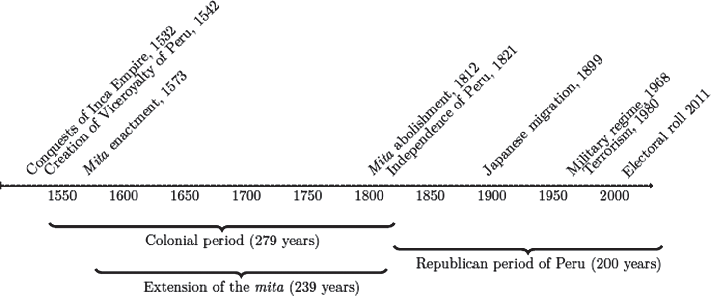
Figure 1 MAIN HISTORICAL EVENTS RELATED TO THE mita
Notes: The timeline displays a list of the main historical events related to the mita, from the conquest of the Inca Empire to its abolishment. It also locates historical events of the Republican era of Peru that we exploit in this article. The stated year refers to the start year of the event.
Source: See text for the section on “Historical background.”
Mita
The mita was a forced labor system designed by Toledo to allocate indigenous labor to mines and refineries. Specifically, 16 provinces of modern-day Peru and Bolivia (over 200 indigenous districts) were chosen to provide one-seventh of their male labor force each year (Cole Reference Cole1985, p. 3; Tandeter Reference Tandeter1983, p. 3; Bakewell Reference Bakewell1984, p. 83). The wage paid to an average indigenous person forced to work under this mandatory regime is estimated at somewhere between a third and a half of the wage received by ordinary laborers (Cotler Reference Cotler2005, p. 54). The most frequent destination by far for these workers was the Potosí mine, the largest source of silver in the Spanish Empire. According to Sánchez-Albornoz (Reference Sánchez-Albornoz1988, p. 194), the initial mita workers in Potosí numbered 13,400, while mita workers in Huancavelica—the second most important destination—numbered at most 3,200. Indeed, in the first half of the seventeenth century, Potosí was the most productive silver mine in the world (Tandeter Reference Tandeter1981, p. 99).
In order to gather information for the implementation of mita, Toledo organized a general census the previous year (Census of 1572), which recorded 1,077,697 indigenous people (Cole Reference Cole1985, p. 2). The mita was established by an arbitrary boundary that divided the territory into mita and non-mita areas (see the map in Online Appendix A). The border was established according to two criteria: elevation and distance to the Potosí mine. Most of the selected communities were located in the colder highland area (Sánchez-Albornoz Reference Sánchez-Albornoz1983, p. 32). Since the Potosí mine was situated over 4,000 meters above sea level (13,000 feet), mine operators needed workers acclimated to the harsh weather conditions. Many historians have also noted that administrative costs, such as transportation and enforcement costs, increased as distance to the mines grew. In fact, the migration was not limited to individuals but included entire families (Gil Montero Reference Gil2013). The trip from the province of Chucuito to Potosí is an illustrative example: it took two months and involved 7,000 people (including women and children) with the help of 40,000 llamas (Cotler Reference Cotler2005, p. 54).
According to historical evidence, the mita caused a population collapse in the subjected area for two reasons. First, many of the indigenous people who were forced to work died because of the harsh labor and weather conditions in the mines. The Indian chronicler Guaman Poma de Ayala (Reference Guaman Poma1615, fol. 529–37) describes in dramatic terms how a great number of native people died in the mines due to the poor labor conditions and harsh punishments (see one full-page drawing from the autograph manuscript in Online Appendix A). Bakewell (Reference Bakewell1984, p. 3) describes the area as cold, dry, and almost uninhabitable because of its hostile climate. Second, the mita created incentives for emigration. Even though an indigenous person that abandoned his village would lose his land, he would still have found it attractive to free himself of mita obligations by permanently leaving his district of residence. The usual way to achieve this was by not returning to his original community once a tour of duty was fulfilled, relocating instead to the city to work as an unskilled laborer (Lockhart Reference Lockhart1982, p. 264). Apart from avoiding being drafted a second time, indigenous workers in Potosí had two additional disincentives to return (Sánchez-Albornoz Reference Sánchez-Albornoz1983, p. 42). First, they feared returning to find their land uncultivated and unsown. Extended families took care of the land of those indigenous who were drafted at the beginning, but the difficulties associated with doing so increased with each mita cycle. Second, since they had not participated in collective activities during their absence, they lost any rights to the surplus they would otherwise have enjoyed. As a result, many indigenous people went from being transitory migrants to permanent migrants. Another way to escape from mita obligations was simply to relocate to a district not subject to mita. This strategy was less common, but still possible according to the memoirs of the Viceroy La Palata: “To get rid of these annoyances, the Indians have found the easiest path across the Andes… because only by standing at the closest province that was not included in the mita, were they exempt from this obligation” (Sánchez-Albornoz Reference Sánchez-Albornoz1983, p. 46).
Many viceroys took note of the depopulation and, concerned about the sustainability of the mita, ordered population counts in the subjected area. The Viceroy Chinchón found a male depopulation on the order of 66 percent in 1633; the Viceroy Alba de Liste documented a decrease of 80 percent in 1663 (Crespo Rodas Reference Crespo Rodas1955–56, p. 181); and the Viceroy La Palata and Viceroy La Monclova (1684–1692) found a reduction of 45 percent (Sánchez-Albornoz Reference Sánchez-Albornoz1983, p. 37). These percentages are all before-and-after estimations, where the baseline is the census ordered by Toledo in 1572. As explained previously, these estimations have serious flaws, which we try to overcome in this study. Historians also suggest a link between the migration generated by mita and the emergence of a new social group among the indigenous called forasteros (foreigners). They lived on Spanish farms or indigenous districts distant from their native region and organized themselves becoming small-scale traders, artisans, and farm employees. According to Tandeter (Reference Tandeter1983, p. 87), they made up around 40 percent of the total indigenous population.
The mita introduced by Toledo in 1573 lasted almost 240 years until its abolishment in 1812. Contrary to what one might expect, this long-lasting institution experienced only small reforms over this period. Viceroy Toledo, for instance, was aware of migration, but he had hoped to lure the indigenous back into their districts of origin. Viceroy La Palata attempted to incorporate the forasteros into the mita draft and to enlarge the subjected region as well. However, these efforts were met with great opposition, and for the most part, went unimplemented. Viceroy Monclova considered abolishing the mita but ultimately chose to maintain it. Sánchez-Albornoz (Reference Sánchez-Albornoz1983, p. 43) explains that the order introduced by Toledo lasted less because of its intrinsic merits than because of the rigidity of the colonial system.
Introduction of Surnames
The inhabitants of Peru, before the Spanish conquest in 1532, used single names with no surnames (Garcilaso de la Vega Reference Garcilaso de la Vega1609, p. 28). The first Quechua grammar, compiled by the Dominican missionary Domingo de Santo Tomás, reports that natives received a name twice in their lives (de Santo Tomás 1560, pp. 156–57). The first name was assigned at birth by parents, who were inspired by a situation or event linked to their child’s birth: a gesture made by the baby soon after being born, an activity is undertaken by the father at that time of birth, a word said by the mother upon first seeing her child, or, perhaps, the name of an animal. Another name was imposed in adulthood, which replaced the previous one. This was traditionally the name of another person, such as the father, the grandfather, or an important member of the lineage. In this regard, the chronicler Guaman Poma de Ayala (Reference Guaman Poma1615, fol. 65) explains that some ancestors with animal names were awarded for bravery in combat. Siblings did not share the same name.
The introduction of surnames to Peru came along with the conversion of indigenous people to Christianity. This process began as soon as the Spanish arrived in 1532, as it was thought to provide the moral justification for their conquest. According to the Spanish Dominican friar Bartolomé de las Casas, “the only way in which the Spanish Crown could occupy the Americas without endangering the King’s hopes for salvation was to convert the natives to Christianity” (Hemming Reference Hemming1970, p. 288). The first significant action of this process was the mass baptism of indigenous peoples, who were ordered to immediately cease all idolatrous practices and rituals that went against Church law (First Council of Lima, 1551). The Jesuit Blas Valera confirms the Indians were given baptisms in the first months after the Conquest, without catechism or doctrinal instruction of any kind (Kubler Reference Kubler and Julian1946, pp. 395). Hemming (Reference Hemming1970, p. 309) also observes that “They flocked to mass baptisms even if they understood almost nothing of the crude interpreting of Spanish sermons.” Mass baptisms were widespread and relatively quick, but conversions took more time. Hiding beneath many indigenous customs and traditions were pagan cults considered idolatry by the Spanish priests.
A consequence of baptizing the indigenous population was the identification of individuals through first name and surname. While there is no evidence of a direct mandate specifying how first name and surname were to be established, the first name was typically Hispanic (often following the calendar of saints or similar criteria); the surname was typically an ethnic name. Hence, most of the surnames are related to the community of origin, defined by racial, linguistic, religious, and kinship affinities. In fact, the chronicler Garcilaso de la Vega (Reference Garcilaso de la Vega1609, p. 28) asserts that the assigned surnames contain information on the origin of the indigenous person, and uses the word surname as a synonym of “caste” throughout his famous work Comentarios Reales de los Incas. It is sometimes possible to find indigenous people who took on their original name as a surname.Footnote 5 One also finds cases of indigenous people receiving an Hispanic surname after their encomendero.Footnote 6
The baptisms and consequent assignment of surnames were, as one could expect, a gradual process that was not completed when the mita was introduced by Viceroy Toledo in 1573. However, this viceroy conducted an important census in 1572 with the specific purpose of collecting information for the assignation of mita obligations. It is reasonable to assume that significant progress was made with the identification process during the census because it was essential for the collection of taxes.
CONCEPTUAL FRAMEWORK
An important feature of both Anglo-Saxon and Hispanic naming conventions is that surnames are inherited from the father (i.e., the surname of the father is passed down). We construct two indicators from current surnames to reveal past changes in the size of the population: the number of surnames and the number of exclusive surnames. We define an exclusive surname as one found solely in one location, in contrast with a common surname or name found in more than one location. We now proceed to analyze the effects of fertility, mortality, and migration shocks on our indicators and to explain why they reveal the effect of mita on past population. Online Appendix B presents a formal stochastic model based on the GW process along with simulations providing support for our claims.
Population Changes and Surnames
We start by explaining the effects of fertility and mortality. We apply our reasoning to a simplified situation in which there are two areas, A and B. Consider a shock to mortality that exclusively affects A (the same analysis holds for a shock to the fertility of opposite sign). Panel 1 in Table 1 presents the four cases that arise when a family experiences this shock by combining two possible kinds of surnames (exclusive or common) and two possible types of impacts: total death, which we define as a process in which all individuals with the same surname die before reproduction, or live long but do not reproduce; and partial death, a process in which some individuals with the same surname bear zero offspring and others reproduce. The main columns correspond to the effect caused by the shock to the number of surnames and number of exclusive numbers, respectively. An upward-pointing arrow signifies an increase; a downward arrow signifies a decrease; a dash indicates no effect.
Table 1 THE EFFECT OF POPULATION CHANGES ON SURNAME INDICATORS

Notes: The table presents the effect of mortality and migration on number of surnames and number of exclusive numbers in a context of two areas, A and B. Panel 1 shows the effect of a mortality increase or out-migration from area A to an outside location. Panel 2 shows the effect of migration from A to B. Every line represents one out of all possible cases. An upward arrow signifies an increase; a downward arrow signifies a decrease; a dash indicates no effect.
Source: See text for the section on “Conceptual framework.”
Our first claim is that a mortality increase in A (or a fertility decrease), when it generates total deaths, reduces the number of surnames in area A and has no effect in area B. At the same time, this shock decreases the number of exclusive surnames in area A and raises it in area B. We support these statements with a case-by-case analysis. The first row of Panel 1 shows the case of a family with an exclusive surname experiencing total death. As the surname disappears in A, the number of surnames and exclusive surnames both decrease there. Neither indicator changes in B, where the surname is absent. The second row presents the case of the total death of a family with a common surname, which is more subtle. This surname disappears from A and, at the same time, becomes exclusive in B. The third and fourth rows present the case of partial death for a family with an exclusive and common surname, respectively. As some individuals of the family reproduce, the surname survives, and the indicators do not change.
Notice that our indicators are not sensitive to a mortality increase that generates only partial deaths because a key element for a change is that no family member remains in A. What conditions does a mortality increase have to fulfill to produce such an extreme situation? First, the shock must take place in the context of few people for each surname. Since the number of people per surname tends to grow exponentially, this last condition is fulfilled if the shock affects the first generations. For this reason, we affirm that the surname indicators detect changes in past population size. Second, the shock has to be large enough to include all family members. Third, the shock has to spread over a number of generations until it reaches all family members.
Our second claim is that a mortality decrease in A (or a fertility increase) does not raise the number of surnames or the number of exclusive surnames in either location. Since the stock of surnames is fixed, this shock only increases the number of individuals per surname. An important consequence of this is that, once a mortality increase in A affects the number of surnames and exclusive surnames in A, these indicators do not return to original levels. The death of a surname is irreversible.
Notice the surname indicators are constant over time, except after some shocks of specific sign (i.e., there is an asymmetry in the surnames dynamics). A fertility increase or a mortality decrease does not change them at all because the set of surnames is fixed. A fertility decrease or a mortality increase does reduce them if the shock is relatively old, large, and long. Moreover, once this shock ends, the surname indicators do not change. We will later discuss why these features favor the use of current surnames over population size to reveal past mortality displacement after mita.
We now turn to analyze the effect of migration. Consider a situation in which there are two areas A and B, but this time there is a one-way migration flow from A to two alternative destinations. Panel 1 of Table 1 represents a migration flow from A to a location different from B, while Panel 2 represents a migration flow from A to B. Each panel shows the four cases that arise by combining two possible kinds of surnames (exclusive or common) and two possible types of migration: total migration, in which all members of a family migrate; and partial migration, in which some members stay.
Our third claim is that a migration flow from A to a location different from B, when it generates total migrations, decreases the number of surnames in area A and has no effect in area B. At the same time, this shock decreases the number of exclusive surnames in area A and increases it in area B. This claim can be supported using exactly the same case-by-case analysis of a mortality increase in A. Hence, in a similar vein, partial migrations do not change our indicators; and, for a migration flow to affect our indicators, it needs to be large, long, and early.
Our fourth claim is that a migration flow from A to B decreases the number of surnames in area A and increases it in area B. The first main column of Panel 2 shows the case-by-case analysis that sustains our claim. The first row considers the case of a family with an exclusive surname that migrates totally. In this case, the number of surnames in A decreases because no family member stays, while the number of surnames in B increases because no one there had that surname previously. The second row shows a family with a common surname under conditions of total migration. The number of surnames in A decreases again, but the number of surnames in B remains the same because the surname was already present there. The third row represents a partial migration of a family with an exclusive surname. We do not observe any change in the number of surnames in A because some family members stay; however, the number of surnames in B increases because the surname is locally absent. The fourth case, partial migration of a family with a common surname, does not affect the number of surnames, either in A or in B. We complete the fourth claim by stating that the migration flow from A to B makes the number of exclusive surnames decrease in A and increase in B. This is not merely an extension of the previous claim because the number of surnames and the number of exclusive surnames are not proportional. The second main column of Panel 2 shows the results of the same case-by-case analysis we have used thus far.
Note, then, that migration can also alter surname indicators. On the one hand, migration to an outside location changes them subject to comprising entire families. As in the case of a fertility decrease or mortality increase, the shock would need to be old, large, and long. On the other hand, migration from A to B changes our indicators not only in the case of total migration but also in the case of partial migration. However, while total migration affects them in any case, partial migration does so only if the families involved have exclusive surnames. A final observation that holds for both types of migration is that, once the flow ends, the surname indicators do not change.
Surnames and the Case of the mita
We use the surname indicators to overcome the lack of historical population data to study the effect of mita on population size. The historical evidence indicates that this forced labor system affected mortality due to the long journeys to the mine as well as the working conditions. In terms of our conceptual framework, this is equivalent to a mortality decrease in area A. It also suggests mita caused out-migration, either of indigenous people who did not return once their duty was fulfilled or because they left their location of residence. These categories appear in our framework as migration from A to a location different from B and as migration from A to B, respectively. The historical evidence further indicates that these processes were large in scale, taking place immediately after the enactment of the mita and lasting for about 240 years. These are the three conditions required for the shocks to have an impact on our indicators. Hence, the mita is likely to have shocked our surname indicators.
We also propose surname indicators to address the fact that too much time has passed to use the current population size. A corollary of the previous analysis is that the surname indicators do not have a fixed relationship with population size, either over time or between localities. While they tend to be stable and have a restricted sensitivity to shocks, population size is sensitive to all possible mortality and fertility shocks (whether they are positive or negative, or small or large) and migration flows (whether they involve exclusive surnames or not). In order to explain why this contrast favors the use of surnames, we simplify the evolution of population size to four scenarios. Assume a difference in current population size between the subjected and exempted areas. This may indicate that the mita caused a difference in past population size that has endured over time (Scenario 1). But this might also mean it did not cause this difference but instead, persistent differential living conditions were responsible (Scenario 2). If that were the case, high household consumption in the exempted area could have raised birth rates after mita, but the surname indicators would not have changed. It is also possible that low household consumption in the subjected area could have lowered birth rates after mita, but surname indicators would have stayed the same or decreased much less because entire families rarely disappear without a shock of the characteristics of mita. Assume now no difference in current population size. This may indicate mita did not cause a difference in past population size (Scenario 3). But this would also be consistent with an effect on past population size that faded over time due to increased fertility (Scenario 4). The surname indicators would not have recovered their original level because the death of a surname is irreversible. Online Appendix B presents simulations illustrating the four scenarios. In sum, by looking at surnames, we neutralize fertility increases and mortality decreases as endogenous responses that may obscure the effect of mita, and we mitigate fertility decreases and mortality increases. As surnames do not set aside reverse migration as a confounder, we will later explore evidence of post-mita migration flows.
We end this section by acknowledging three limitations of our indicators additional to those mentioned in the introduction. First, their focus is limited to the male population. Despite the fact that the mita exclusively targeted men, it affected both male and female populations. As mentioned before, migration to the mines included entire families. Unfortunately, we cannot make inferences about the female population from our indicators. Since the first surname is inherited from the father and the second is inherited from the mother, the former endures, and the latter survives only one generation. In spite of this limitation of current surnames, providing evidence of a male population decrease does provide indirect evidence of a general population decrease. This is because a decrease in either the male or the female population will result in a general population decrease from the next generation onwards. Second, our indicators are not able to disentangle a shock to fertility, a shock to mortality, and mass migration. Historical evidence indicates that mita generated both mortality displacement and mass migration, but we are unable to go further with our indicators. Third, since each of our indicators is a count of surnames by geographical unit, the final database being analyzed has a much smaller sample size than the original one. Working with a small sample implies methodological challenges. Since we cannot show consistent non-parametric RD estimates based on the optimal bandwidth of Calonico, Cattaneo, and Titiunik (Reference Calonico, Cattaneo and Titiunik2014), we conduct a semiparametric RD design and present the robustness of the results to bandwidth choice.
DATA
We use an RD approach similar to the one proposed by Dell (Reference Dell2010), restricting our analysis to the same zone examined in her study. While most of the mita border coincides with the Andean precipice (with communities at higher elevation included and those at lower elevations exempted), Southern Peru has segments that transect the Andean region. Dell focuses exclusively on these segments to avoid a discontinuous change in elevation and because ethnic distribution and other observables at both sides of the border are statistically identical there. This homogeneity favors the assumption that all relevant factors besides the treatment vary smoothly at the mita boundary, as required by the RD approach. The map in Online Appendix A shows the mita borders and the segments considered in this study.
Our district-level data is constructed from two sources (Carpio and Guerrero Reference Carpio and María2021). We employ the Peruvian Electoral Roll of 2011 (ER 2011) to construct the indicators explained in the previous section at the district level. The ER 2011 is the list of potential voters used during elections for President and Vice Presidents for the period 2011–2016, as well as for members of the Peruvian Congress. It contains the names, surnames, identification numbers, genders, and districts of residence of the voting population, regardless of whether they exercise their right to vote. The voting population is composed of all citizens aged 18 and older. We also use the data provided by Dell (Reference Dell2010),Footnote 7 which includes the list of mita and non-mita districts, their latitude and longitude, average altitude, average elevation, distance to the mita boundary, distance to the Potosí mine, and the distance to Huancavelica. We link both databases through the district names. The ER 2011 was provided by the National Office of Electoral Processes exclusively for the area under analysis, that is, the departments of Apurimac, Ayacucho, Arequipa, Cusco, and Puno. According to the National Registry of Identification and Civil Status, the number of Peruvians identified by an identification number has grown substantially in recent years, from a coverage rate of 62 percent in 2006 to 97 percent in 2011. Importantly, if we restrict the analysis to the population aged 18 and over, the coverage rate reaches 100 percent in 2010 (RENIEC 2011). This explains why we have selected ER 2011 from among the other Peruvian electoral rolls.
Peru follows the Hispanic naming convention. Individuals have two surnames: the first is inherited from the father (his first surname), the second is from the mother (her first surname). In contrast to females in Spain, who rarely modify their surnames when they marry, married females in Peru may voluntarily add their husband’s surname to their own.Footnote 8 This works by replacing their second surname with the first surname of their husbands preceded by the word “de,” which means “of.” From 2009 on, the procedure has implied maintaining their two surnames and adding their husbands’, preceded by the word “de.”Footnote 9 In order to avoid any possible bias, we focus exclusively on the first surname (henceforth “surname”), which is not subject to any modification due to changes in marital status.
The ER 2011 provides information on the 1,383,523 inhabitants over the age of 18 in the 299 districts of analysis, with a total of 16,571 surnames represented. A small number of the most frequent surnames make up a large percentage of the population. The 10 most popular surnames account for around 18 percent of the names of the sample population. At the same time, a large number of low-frequency surnames are found among the population. Hence, as we will confirm later, distributions are heavily skewed to the right. This is a well-known feature of surname distribution (Guell, Rodríguez Mora, and Telmer 2014), observable after several generations have passed since their initial use.
We classify the set of 16,571 surnames according to the definitions of our conceptual framework. Figure 2 presents the results. We must go beyond the assumption of two areas to apply the definitions. The political organization of Peru consists of (in descending order): departments, provinces, and districts. The mita and the non-mita areas have, of course, several districts within them. We then propose two indicators according to the geographic scope of reference. The first is “district-exclusive surnames,” the number of names found in only one district. For instance, the surname Chancos is found in the district of Huancapi in the Department of Ayacucho and is not found in any other district in the sample. In the dataset, 7,548 surnames are district-exclusive (46 percent). This indicator goes along with the objective of comparing districts close to the boundary, but it has the flaw of being sensitive not only to migration from a mita to a non-mita district but also to migration between mita districts or between non-mita districts.
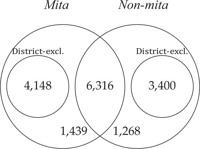
Figure 2 CLASSIFICATION OF THE ER 2011 SURNAMES
Notes: The Venn diagram presents the classification of the 16,571 surnames that appear in the ER 2011 (departments of Apurímac, Ayacucho, Arequipa, Cusco, and Puno) in accordance to the definitions of the conceptual framework. The figures represent the number of elements of each subset.
Source: Peruvian Electoral Roll of 2011.
The second indicator is “area-exclusive surnames,” the number of names in a district that are exclusive to the area (mita or not) to which the district belongs. In other words, to be exclusive to a given area, a surname needs to be absent, not from any other district, but only from the other area. Consider, for instance, the case of the surname Achapuma, which is found in four mita districts (Juliaca, Sicuani, Mosoc Llacta, and Acopia), but it is not found in any non-mita district. In the dataset, 10,255 surnames are area-exclusive (62 percent) and 6,316 are common (38 percent).Footnote 10 This second indicator is not sensitive to migration within areas. Notice that a district-exclusive surname is always an area-exclusive surname. In our examples, Chancos is an exclusive surname according to both definitions; Achapuma is an area-exclusive surname but not a district-exclusive surname. Table A.1 of Online Appendix A presents the 20 surnames with the largest population within each type (common, area-exclusive, district-exclusive) and area (mita and non-mita).
Once we classify every surname, we use the list of surnames located in each district to count them at the district level.
ESTIMATION FRAMEWORK
In order to examine the effect of mita on past population size, we apply an identification strategy very similar to that proposed by Dell (Reference Dell2010) but using our indicators as outcomes. This involves using an RD to exploit the discrete change at the boundary of the subjected region: communities on one side were forced to send parts of their adult male population to work in mines; communities on the other side were exempt. The treatment is a deterministic and discontinuous function of longitude and latitude. Hence, provided that mita and non-mita districts are comparable near the arbitrary boundary, differences in surnames today would indicate a change in the past population size. The equation to estimate is:
 $${m_{db}} = \alpha + \gamma mit{a_d} + X{'_d}\;\beta + f(geographic\;locatio{n_d}) + {\phi _b} + {\varepsilon _{db}},$$
where m db is the surname indicator for district d along segment b of the mita boundary; mita
d is a dummy equal to 1 if district d was included in mita and 0 otherwise;
 $${ X_d}$$
is a vector of covariates, which includes weighted average elevation and slope of district d; f (geographic location d
) is the RD polynomial, which controls for smooth functions of geographic location; and
$${ X_d}$$
is a vector of covariates, which includes weighted average elevation and slope of district d; f (geographic location d
) is the RD polynomial, which controls for smooth functions of geographic location; and
 $${\phi _b}$$
is a set of boundary fixed effects. The boundary has been divided into four equal-length segments b, and
$${\phi _b}$$
is a set of boundary fixed effects. The boundary has been divided into four equal-length segments b, and
 $${\phi _b}$$
identifies which of these four is the closest to the capital of district d. This variable is used to compare observations in close geographic proximity. The parameter of interest is γ.
$${\phi _b}$$
identifies which of these four is the closest to the capital of district d. This variable is used to compare observations in close geographic proximity. The parameter of interest is γ.
A semiparametric RD estimation is used to distinguish the effect of mita from the smooth effects of geographic location.Footnote 11 The sample is limited to districts within 100, 75, and 50 km of the mita boundary. In our baseline specification, f (geographic location d) is a quadratic polynomial of longitude and latitude that includes interactions with mita
 $$(x + y + {x^2} + {y^2} + xy\; + \;x \cdot mita\; + \;y \cdot mita\; + \;{x^2} \cdot mita\; + \;{y^2} \cdot mita\; + xy \cdot mita)$$
. This polynomial differs from the one used by Dell (Reference Dell2010) in two respects. First, we use a quadratic polynomial rather than a cubic one. As Gelman and Imbens (Reference Gelman and Guido2014) have argued, estimators based on cubic or higher-order polynomials are potentially misleading. Second, we introduce interactions with mita to avoid our results being driven by the stiffness of the polynomial. These interactions resemble the interaction between the forcing variable and the treatment variable in a one-dimensional RD design. This is the method of choice, and we will later subject it to several robustness checks. These exercises include presenting results with the identical polynomial used by Dell (Reference Dell2010).
$$(x + y + {x^2} + {y^2} + xy\; + \;x \cdot mita\; + \;y \cdot mita\; + \;{x^2} \cdot mita\; + \;{y^2} \cdot mita\; + xy \cdot mita)$$
. This polynomial differs from the one used by Dell (Reference Dell2010) in two respects. First, we use a quadratic polynomial rather than a cubic one. As Gelman and Imbens (Reference Gelman and Guido2014) have argued, estimators based on cubic or higher-order polynomials are potentially misleading. Second, we introduce interactions with mita to avoid our results being driven by the stiffness of the polynomial. These interactions resemble the interaction between the forcing variable and the treatment variable in a one-dimensional RD design. This is the method of choice, and we will later subject it to several robustness checks. These exercises include presenting results with the identical polynomial used by Dell (Reference Dell2010).
The strategy requires districts just outside the boundary to be an appropriate counterfactual to those just inside of it. This requires that all relevant factors vary smoothly at the discontinuity. Dell (Reference Dell2010, pp. 1871–75) examines this assumption in four important dimensions, to the extent that the available data allows it. First, she considers geographical variables, analyzing elevation and slope, which determines climate and crop choice in Peru. The data cover all relevant districts. Second, she looks at ethnicity, comparing the current percentage of the population whose primary language spoken in the home is an indigenous one. The data come from a representative household survey. Finally, she examines pre-mita population and economic variables, including the size and structure of the population, as well as local tribute rates and allocation of tribute revenues. The data come from the 1572 Census of Toledo, one year before the mita enactment. The use of this census involves two problems. First, as with all colonial censuses, the colonial officials conducting the census had incentives to misrepresent actual counts. In the case of this particular census, this potential worry does not invalidate the use of an RD design because it was taken before the mita enactment. One can assume that incentives to defraud were similar on both sides of a border yet to be defined. Second, the data cover only a tiny fraction of the relevant districts. This certainly calls into question its utility for testing whether the mita and non-mita districts are comparable. We believe that, despite its serious limitations, this data is the best historical pre-mita source available.
Given the nature of our study, we focus our attention on the population and economic variables from the 1572 Toledo inspection. We want to corroborate, to the extent that the limited number of observations allow, that in 1572 treated and control groups had similar populations in terms of size, structure, and well-being. This will be prima facie evidence that the types of surnames (Spanish or Indigenous) were also similar. Table 2 presents the means of these variables by mita status and tests whether they are statistically different. The first three columns focus on observations that are 100 km from the mita boundary, while the following columns restrict the boundary to 75 and 50 km. The first row shows the size of the population. There are no significant differences between mita and non-mita districts before the enactment of the mita.Footnote 12 Rows 2 to 4 provide information on the population structure, with no significant differences seen in the rates of men, women, or boys. The fifth row of Table 2 shows the average tribute contributions per adult and finds no significant difference. This is the best available proxy for well-being. In addition, rows 6 to 9 present the relative share of the tribute revenues of the Spanish and Indigenous Mayors and find no significant difference. We provide this information to contrast contribution levels to Indigenous Mayors with those of the Spanish population, which includes nobility, priests/clergy, and judges.Footnote 13
Table 2 SUMMARY STATISTICS FOR 1572 DEMOGRAPHICS BY mita STATUS

Notes: The unit of analysis is the district. The table presents means and differences in means, and tests whether they are statistically different. The first three columns present t-tests for observations that are 100 km from the mita boundary; the following columns restrict the boundary to 75 and 50 km. Standard errors for the difference in means are in parentheses. Differences that are significantly different from zero are denoted by: *** p < 0.01, ** p < 0.05, * p < 0.1.
a This variable is the natural logarithm of average tribute contributions per adult.
Sources: Data from Dell (Reference Dell2010). The original source is the 1572 census ordered by Viceroy Toledo.
The context of recently assigned surnames and the lack of discontinuity in the population variables make it reasonable to assume that the pre-mita distributions of surnames vary smoothly at the boundary between the mita and non-mita districts.
RESULTS
Preliminary Evidence
Table 3 provides summary statistics for the three proposed indicators. It presents the means of these variables by mita status and tests whether the differences are statistically significant. Each of the three groups of three columns focuses on districts whose proximity to the mita boundary is 100 km, 75 km, and 50 km, respectively. The first row shows the logarithm of the number of surnames by the district. A significant negative difference exists between mita and non-mita districts, which increases as the analysis focuses on the districts nearer to the boundary, ultimately reaching 28 log points. The second row gives the logarithm of the number of exclusive surnames by the district. Again, the closer to the mita boundary, the larger the negative difference. At the smallest bandwidth, the number of district-exclusive surnames is 32 log points lower in the mita districts than in the non-mita, a difference that is statistically significant. The third variable presents the logarithm of the number of area-exclusive surnames, which follows a similar pattern. The negative difference between mita and non-mita reaches 43 log points for the districts closest to the boundary, which is also statistically significant.
Table 3 SUMMARY STATISTICS FOR SURNAME INDICATORS BY mita STATUS

Notes: The unit of analysis is the district. The table presents means and differences in means, and tests whether they are statistically different. The first three columns focus on observations that are 100 km from the mita boundary; the following columns restricts the boundary to 75 and 50 km. Standard errors for the difference in means are in parentheses. Differences that are significantly different from zero are denoted by: *** p < 0.01, ** p < 0.05, * p < 0.1.
a This variable equals ln(number of district-exclusive surnames + 1). This transformation in done to preserve the entire sample because some observations are equal to zero (seven obs. in the larger bandwidth, five and two in the subsequent bandwidths).
Sources: Peruvian Electoral Roll of 2011 and data from Dell (Reference Dell2010).
We now examine the distribution of surnames by area. Panel A of Figure 3 shows density functions for the number of surnames separately for those falling inside and outside the mita area. It limits the sample to those districts within 50 km of the mita boundary. As anticipated in the data section, distributions are skewed to the right. The distribution of those districts subjected to mita shows a higher concentration in lower values than the distribution of those that are not. Panels B and C repeat this exercise, using the two definitions for the number of exclusive surnames as dependent variables. While the shift is small for district-exclusive surnames, it is larger for area-exclusive surnames.
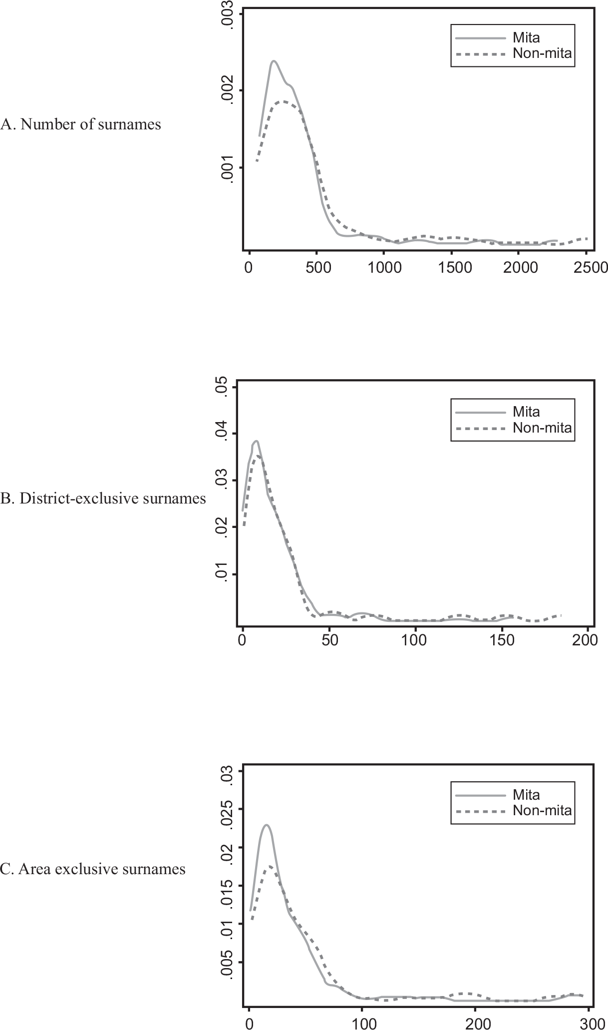
Figure 3 DENSITY ESTIMATES OF SURNAME INDICATORS BY mita STATUS
Notes: The unit of analysis is the district. The figure presents kernel density estimates for number of surnames, number of district-exclusive surnames, and number of area-exclusive surnames, respectively. It focuses on observations that are 50 km from the mita boundary.
Sources: Peruvian Electoral Roll of 2011 and data from Dell (Reference Dell2010).
The results of Table 3 and Figure 3 show, with simple statistical indicators, that mita is associated with differences in the number of surnames. It is comforting to see that these differences do not rely on the decisions we make for Equation (1) (i.e., RD polynomial, control variables). Note further that these differences widen as we approach the border. This suggests that the point estimates for γ in Equation (1) will be even larger. We now turn to the econometric analysis.
Estimation Results
Table 4 presents the main results of the econometric estimation: point-estimates for γ from Equation (1) and robust standard errors. Each horizontal panel of Table 4 corresponds to the natural logarithm of the three proposed indicators as dependent variables: number of surnames, number of district-exclusive surnames, and number of area-exclusive surnames. The columns correspond to three possible sub-samples: districts within 100 km, 75 km, and 50 km of the boundary. Following Dell (Reference Dell2010), we exclude Metropolitan Cusco from the main part of our analysis, the concern being that its current level of development may be determined by its status as the former capital of the Inca Empire. Metropolitan Cusco is composed of two mita and eight non-mita districts.Footnote 14 We will later provide results incorporating the ten Metropolitan Cusco districts back into the analysis.
Table 4 RD ESTIMATES OF THE mita EFFECT ON SURNAME INDICATORS

Notes: The unit of analysis is the district. All regressions are multidimensional RD using a quadratic polynomial of latitude and longitude that includes interactions with mita. All regressions include geographic controls and boundary segment fixed effects. Robust standard errors are in parentheses. Coefficients that are significantly different from zero are denoted by: *** p < 0.01, ** p < 0.05, * p < 0.1.
a This variable equals ln(number of district-exclusive surnames + 1). This transformation in done to preserve the entire sample, because some observations are equal to zero (seven obs. in the larger bandwidth, five and two in the subsequent).
Sources: Peruvian Electoral Roll of 2011 and data from Dell (Reference Dell2010).
The first row of Table 4 estimates that the mita districts have from 43 to 47 log points fewer surnames than the non-mita districts. The second row shows that the mita districts have from 60 to 73 log points fewer district-exclusive surnames than the non-mita districts. The third row shows that the difference in the number of exclusive surnames following the broader definition ranges from 93 to 97 log points. Note that for each variable, the point estimate remains stable as the sample is restricted to districts closer to the mita boundary. Moreover, the nine-point estimates are statistically significant at the 1 percent or 5 percent level. Table A.2 in Online Appendix A estimates the same specification as Table 4 but using a bootstrapping technique. The results are essentially the same when we use random resampling.
In order to show our results graphically, we contrast the data values and the predicted values within a map of the area of study in Figure 4. There is one subfigure for each of our three indicators built from surnames. Every map includes the boundary dividing the territory: the intermediate zone is the mita area, while the upper and lower zones are the non-mita area. The data and predicted values are contrasted as follows. First, every map includes one dot for each district, and the color of this dot represents the data value. Each dot is located in the latitude and longitude of the district capital, but its color represents the data value for the whole district. Second, every map includes a background that shows predicted values. The background is a finely spaced grid of latitude and longitude, where the color of every tiny square represents the predicted value from Equation (1) using our baseline specification. Figure 4 is useful for two reasons: First, we can assess how our equation fits the actual values by comparing the color of the dots and the color of the closest background; second, we can observe the discontinuity by contrasting the shades inside and outside the mita boundary. Notice that this contrast is sharper in the northern than in the southern boundary, which is probably due to the smaller size of the pre-mita population in the northern zone.Footnote 15 We do not pursue this interesting heterogeneity any further due to our small number of observations.

Figure 4 MAP OF THE AREA OF STUDY WITH DATA AND PREDICTED VALUES OF SURNAME INDICATORS
Notes: The unit of analysis is the district. Panels A, B, and C show maps for number of surnames, number of district-exclusive surnames, and number of area-exclusive surnames, respectively. Every dot is located in the latitude and longitude of the capital of one district. The color of the dot represents the data value of the district. The background shows predicted values from Equation (1) using our baseline specification. The white area corresponds to the excluded districts contained by Metropolitan Cusco, the former capital of the Inca Empire.
Sources: Peruvian Electoral Roll of 2011 and data from Dell (Reference Dell2010).
Table 4 and Figure 4 confirm econometrically what Table 3 and Figure 3 suggest, that is, that mita introduced important differences in the number of surnames and the number of exclusive surnames. This confirms quantitatively that mita caused a population collapse in the subject area. We will later show that these results are robust to a series of tests.
We have recognized from the beginning that, although our methodology provides evidence of the existence of a population decline in the past, it does not give an exact estimator of that decline. However, it is possible to obtain a rough estimate for the lower bound of the decline. The population difference between the mita and non-mita areas caused by this colonial institution would exceed 47 log points, which corresponds to the smallest bandwidth in Table 4.
WHEN DID THIS HAPPEN?
The RD design applied on surname indicators has shown that the mita caused a past population decline, but it cannot ascertain when it took place. On the one hand, the population gap may have originated during the years mita was in force (between 1573 and 1812) as a direct consequence of its enactment. This hypothesis is favored by the fact that to have an effect on the surname indicators, mortality and most migration flows must occur when the number of people per surname is low. On the other hand, mita may have first generated the underdevelopment of the mita area, and then this inequality could have generated higher emigration and lower immigration in the mita area after 1812. A reason to explore this hypothesis is that our indicators are not insensitive to some relatively recent migration flows.
Historical evidence suggests that population movements in the Republican era were small in scale, especially if we compare them with those that followed mita. Along similar lines, Dell (Reference Dell2010) provides aggregate statistical evidence in favor of similar patterns of migration between the mita and non-mita areas from 1812 on, which is crucial to defending the RD assumption of no selective sorting across the border. Dell computes district-level population correlations from population censuses, separately for mita and non-mita districts. Consistent with a constant aggregate population distribution, the pair of correlations from 1876 to 1940 are high and similar, as are the pair from 1940 to 1993.
We go one step further here, also presenting microeconometric evidence. We include additional data to analyze post-mita migration flows. We want to know whether mita relates to higher emigration and lower immigration at any point after 1812. We will obtain no statistically significant differences. This is supportive evidence that the substantial change in population size we report should have occurred during mita.
Japanese Migration
Peru was the first Latin American country to accept immigrants from Japan. We access official data concerning the first 18,727 Japanese immigrants, who arrived between the years 1899 and 1941. The data are taken from the “Pioneers” project, promoted jointly by the Japanese Peruvian Association and the Japan International Cooperation Agency. It includes name, surname, prefecture of origin, ship name, and date of arrival.
We build two complementary indicators. The first is “District with a Japanese surname,” a dummy equal to one if the district has at least one surname also present in the database of initial Japanese immigrants. The average is 0.43 for this variable, that is, 43 percent of the sample districts have at least one Japanese surname. The second is “Number of Japanese surnames,” the number of surnames within each district that are also present in the referred database. The average is 0.85. Hence, while the Japanese migrants did not settle in large numbers in the Southern Andes (intensive margin), they managed to cover a good portion of its districts (extensive margin).
We then apply the same estimation of the previous section using these variables as outcomes. The first and second rows of Table 5 present the results. We find no evidence of a significant mita effect in the three possible sub-samples: districts within 100 km, 75 km, and 50 km of the boundary, respectively. One might argue that, even though there is no statistical significance, the estimators are still quite large. This is true, but note that the point-estimates are positive. This is not compatible with less immigration to the mita area due to its underdevelopment.
Table 5 RD ESTIMATES OF THE mita EFFECT ON post-mita MIGRATION INDICATORS

Notes: The unit of analysis is the district. All regressions are multidimensional RD using a quadratic polynomial of latitude and longitude that includes interactions with mita. All regressions include geographic controls and boundary segment fixed effects. Robust standard errors are in parentheses. Coefficients that are significantly different from zero are denoted by: *** p < 0.01, ** p < 0.05, * p < 0.1.
a These variables equal ln(variable + 1). This transformation in done to preserve the entire sample because some observations are equal to zero.
Sources: “Pioneers” project of the Japanese Peruvian Association, 2007 Peru Census, Peruvian Electoral Roll of 2011, and data from Dell (Reference Dell2010).
We complement this result with Table A.3 in Online Appendix A, which presents the means for the two variables by mita status for different bandwidths. This evidence is also incompatible with less immigration to mita districts.
Internal Migration
For a long time after the end of Spanish rule, Peru did not experience any sizable internal migratory movements or population declines. Internal migration maintained low levels until 1950 when economic opportunities prompted farmers and villagers started to migrate to large urban communities (Martínez Reference Martínez1980; León Reference León1980). Urban development was directed mainly towards the coast and especially to the capital, Lima. This process substantially increased after two events. First, the military regime of 1968–1975 contributed to the impoverishment of rural areas. Second, terrorism in Peru forced thousands of people to abandon their rural hometowns during the decade of 1980. This migration wave gradually ended, lasting until the end of the twentieth century. Today, a modest degree of internal migration flows from rural areas to mid-sized cities, not just to the coast or the capital.
We want to observe whether the rural-to-urban migration process, which took place roughly from 1950 to 2000, varied across the mita boundary. We use the 2007 Peru Census, conducted by the Instituto Nacional de Estadística e Informática. We construct a rough proxy for the out-migration ratio by comparing the current district of residence and the district of residence of the mother when the individual was born. We obtain an average of 199 for this variable. Table 5 shows that the point estimate varies greatly from sample to sample: –0.040, 0.075, and 0.168 for districts within 100 km, 75 km, and 50 km of the boundary, respectively. None of these are statistically significant. We interpret this as a lack of evidence of a larger migration to Lima from the mita districts than from the non-mita in the twentieth century. We go further on internal migration to observe whether it varies across the mita boundary in the twenty-first century. We construct proxies for current immigration and out-migration ratios by comparing the districts of residence today and five years ago. We obtain an average of 2.7 percent for the former and 4.7 percent for the latter. Panels D and E of Table 5 show that the point estimates are relatively small, and in any case, not statistically significant.
Online Appendix A explains the construction of these internal migration variables in detail. Table A.3 in this Online Appendix presents averages for these variables by mita status.
Current Population Size
We have shown that the mita opened a substantial gap in past population size between the subjected and no subjected districts; we have also provided suggesting evidence that this change took place during the lifetime of mita. A final natural question concerns what happened afterward. In particular, did this affect endure or fade away? Table A.3 in Online Appendix A presents the means of the number of people in the electoral roll (recall that it includes population aged 18 years and over) by mita status. The differences are small and not statistically significant. We also estimate Equation (1) but using this number as the dependent variable. The last row of Table 5 estimates that the mita districts have from 54 to 63 log points fewer individuals than the non-mita districts. The point estimate remains stable as the sample is restricted to districts closer to the boundary. The evidence then suggests that the gap caused by mita in past population size managed to persist over time. In terms of the four scenarios described in our conceptual framework, the empirical evidence points to Scenario 1 as most likely.Footnote 16
ROBUSTNESS TESTS
We have performed a number of robustness exercises. This section briefly presents their objectives and the results. Online Appendix A explains them in detail.
We have assumed similarity in population structure between subject and control regions pre- and post-mita. We then try to determine whether this assumption can be independently supported by other empirical evidence. First, while Table 2 already presents summary statistics on demographic and fiscal variables, we now estimate Equation (1) using them as dependent variables. Second, in order to address specific concerns about the comparability of treated and control districts, we estimate Equation (1) using different samples: we include the districts of Metropolitan Cusco, exclude the Inca states, and exclude districts whose mita boundaries coincide with rivers.
We also determine whether our most important results are sensitive to the particular bandwidth we have chosen. Rather than focus on our baseline proximity bandwidths of 50, 75, and 100 kilometers distance to the mita boundary, we show how our estimates change when we consider bandwidths of 30 to 100 kilometers in intervals of 5.
We examine robustness to the particular specifications we have used. First, we use different specifications of the RD polynomial f (geographic location d ), including linear and cubic polynomials, as well as the three baseline specifications used by Dell (Reference Dell2010). Second, we use different polynomials of elevation and slope, our main control variables. Third, we introduce two additional control variables: the distance to the Potosí mine, because this was a criterion for the assignment of mita and likely a determinant of out-migration, as well as current population size in order to compare districts of the same population size.
Overall, the sign and the size of the effects seem to be very stable to different bandwidths, different samples, and control variables. When we test the RD polynomial f (geographic location d), the size of these effects may change (but not the sign). We believe this is related to the small number of observations used in all our regressions. The shortage of observations, which also prevented us from developing a non-parametric estimation, is one of the most important limitations in the development of our strategy.
CONCLUSIONS
One of the most representative mental images of the domination of the Spanish crown over the American colonies is that of galleons filled with gold and silver crossing the oceans from Peru to the port of Seville. The exploitation of minerals in the Americas was possible thanks to the forced labor systems imposed by the Spanish crown, of which the mita is a prominent example. Subjecting a significant portion of the indigenous people to this system certainly came at a cost. The decimation of the native-born male population in the subject area was arguably the first, in terms of both time and importance. The qualitative evidence regarding this phenomenon is abundant, but producing quantitative evidence has proved elusive because of the unreliability of colonial population counts, the result of fraudulent manipulation by colonial officials. We provide quantitative evidence that mita did cause a population collapse. We exploit the fact that the aboriginal population of Peru received surnames for the first time as part of mass baptisms conducted after the conquest. We apply an RD design on surnames counts of the current population. The RD design allows us to infer causality, while the surnames allow us to detect the effect of mita on past population size, and to neutralize some of the endogenous responses that affect current population counts. We find a huge difference at the mita border for the number of surnames, area-exclusive surnames, and district-exclusive surnames; we estimate that the reduction in the native-born male population was greater than 47 log points. We also provide suggestive evidence that depopulation took place while the mita was in force and that the population gap managed to last over time. Hence, we hope to shed light on an important question in Latin American historiography.
Our findings are connected to the broader story of Peruvian economic development. The mita effect on population size that we find may have played a crucial role in the long-run consequences of this colonial institution, documented by Dell (Reference Dell2010), for at least three reasons. First, the depopulation caused by mita has persisted up until the present day. Second, historical evidence strongly suggests that the migration caused by mita was selective. Cook (Reference Cook2004, p. 250), for instance, states “Migration was selective: Males of an economically productive age changed residence most often and for the greatest distances. An Indian skilled in a needed craft, for example, might be more successful in an urban environment than in his native village.” To the extent that ability, health, and other characteristics are highly heritable, the initial differences generated by mita could have persisted over many years. Third, if we believe that societies with lower genetic diversity lack some of the traits that are conducive to economic growth, as argued by Ashraf and Galor (Reference Ashraf and Oded2013) and Arbatli et al. (Reference Arbatli, Ashraf, Oded and Marc2020), the diversity evidenced by the number of surnames could help in understanding other aspects of the mita effect.


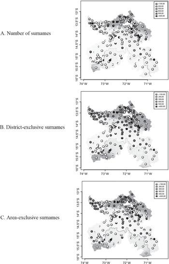


 Open access