AUV Obstacle Avoidance Planning Based on Deep Reinforcement Learning

Abstract

In a complex underwater environment, finding a viable, collision-free path for an autonomous underwater vehicle (AUV) is a challenging task. The purpose of this paper is to establish a safe, real-time, and robust method of collision avoidance that improves the autonomy of AUVs. We propose a method based on active sonar, which utilizes a deep reinforcement learning algorithm to learn the processed sonar information to navigate the AUV in an uncertain environment. We compare the performance of double deep Q-network algorithms with that of a genetic algorithm and deep learning. We propose a line-of-sight guidance method to mitigate abrupt changes in the yaw direction and smooth the heading changes when the AUV switches trajectory. The different experimental results show that the double deep Q-network algorithms ensure excellent collision avoidance performance. The effectiveness of the algorithm proposed in this paper was verified in three environments: random static, mixed static, and complex dynamic. The results show that the proposed algorithm has significant advantages over other algorithms in terms of success rate, collision avoidance performance, and generalization ability. The double deep Q-network algorithm proposed in this paper is superior to the genetic algorithm and deep learning in terms of the running time, total path, performance in avoiding collisions with moving obstacles, and planning time for each step. After the algorithm is trained in a simulated environment, it can still perform online learning according to the information of the environment after deployment and adjust the weight of the network in real-time. These results demonstrate that the proposed approach has significant potential for practical applications.

1. Introduction

The ultimate goal of mobile robot research is to process the data measured by the sensing devices carried by the robot and to achieve completely independent decisions through online processing. In a dynamically changing environment, it is extremely important to plan a reasonable, safe path for a given task. The path planning of autonomous underwater vehicles (AUVs) can be divided into two categories: global path planning based on a completely known environment and local path planning based on an uncertain environment, in which the shape and location of the obstacles are unknown. In recent decades, research in this field has produced many achievements. Global path planning methods include the sampling-based A* algorithm [1] and the rapidly-exploring random tree [2,3]. In addition, there are many intelligent optimization algorithms, such as genetic algorithms (GAs) [4], ant colony optimization (ACO) [5], and particle swarm optimization (PSO) [6], which can also realize path planning. Petru et al. [7] proposes a sensor-based neuro-fuzzy controller navigation algorithm. The control system consists of a hierarchical structure of robot behavior. The authors propose the use of segmented 2-D occupancy maps to use ground-based probability grids for application in mobile robot navigation with collision avoidance in [8]. The authors propose an extended Voronoi transform algorithm that imitates the repulsive potential of walls and obstacles and combines the extended Voronoi transform and the fast marching method to realize the robot’s navigation in a previously undeveloped dynamic environment [9]. These methods can produce excellent results in simulated environments. Nevertheless, it is difficult to obtain a satisfactory path because information about the real environment is incomplete.

The marine environment has various uncertainties, such as floating objects, fish, and ocean currents. In addition, accurate path planning is challenging due to errors caused by approximations and linearization in the modeling of the system. As AUVs have limited energy, designing an AUV path planner to run in real-time in an uncertain environment while avoiding static and uncertain dynamic obstacles is a critical issue.

In a continuous large-scale space, it is difficult to perform obstacle avoidance using only reinforcement learning (RL), as this requires long-term learning and is relatively inefficient. The continuity of the state and action spaces leads to the so-called dimensionality disaster, and traditional RL cannot be applied in any effective form. Although dynamic programming (DP) can be applied to continuous problems, accurate solutions can only be obtained for special cases. Many scholars combine RL with fuzzy logic, supervised learning, and transfer learning to realize the autonomous planning of robots [10,11,12,13]. For example, [10] proposed the use of RL to teach collision avoidance behavior and goal-seeking behavior rules, thus allowing the correct course of action to be determined. The advantage of this approach is that it requires simple evaluation data rather than thousands of input-output training data. In [11], a neural fuzzy system with a hybrid learning algorithm was proposed in which supervised learning is used to determine the input and output membership functions, and an RL algorithm is used to fine-tune the output membership functions. The main advantage of this hybrid approach is that, with the help of supervised learning, the search space for RL is reduced, and the learning process is accelerated, eventually leading to better fuzzy logic rules. Meng et al. [12] described the use of a fuzzy actor-critic learning algorithm that enables a robot to readapt to the new environment without human intervention. The generalized dynamic fuzzy neural network is trained by supervised learning to approximate the fuzzy inference. Supervised learning methods have the advantage of fast convergence, but it can be difficult to obtain sufficient training data.

The authors proposed Q-learning and neural network (NN) planners to solve the obstacle avoidance problem in [14,15,16]. The robot has the ability to implement collision avoidance planning, but the time taken to reach the target point is too long, and the target point cannot always be identified. In practical applications, the robot’s ability to reach the target point is as important as its ability to avoid obstacles.

In the existing literature, there are many research studies in which deep reinforcement learning (DRL) is applied to solve the problem of self-learning. For example, [17] proposed a DRL model that can successfully learn control strategies directly from some high-dimensional sensory input. The authors of [18] developed a DRL approach that adds memory and assisted learning objectives for training agents, enabling them to navigate through large, visually rich environments, including frequent changes to the start and target locations. NNs have been used to perform data fusion from different sensor sources with DRL and then employed for search and pick things [19]. In [20], an improved reward function was developed using a convolutional NN, and the Q-value was fitted to solve the problem of obstacle avoidance in an unknown environment. Long et al. [21] proposed a multi-scenario, multistage training framework for the optimization of a fully decentralized agent-system collision avoidance strategy through a powerful policy gradient. The authors of [22] developed three different deep neural networks to realize the robot’s collision avoidance planning in a static environment. The authors of [23] developed a distributed DRL framework (each subtask passes through the designed LSTM-based DRL network) for the unmanned aerial vehicle (UAV) navigation problem.

Several algorithms take information directly from the original image, without preprocessing, and formulate control strategies through DRL. In [24], the author used CNN and DRL methods to use raw pixels as input to allow the agent to learn navigation capabilities in a 3D environment. For instance, [25] used supervised learning to obtain depth information from a monocular vision image and then used a DRL algorithm to learn a control policy that selects a steering direction as a function of the vision system’s output in the virtual scene before finally applying the policy in actual autonomous driving. In [26], a motion planner based on DRL was proposed in which sparse 10-dimensional range findings and the target position are used as the input and the continuous steering commands as output. The DRL approach seems very promising because it does not require deep learning to obtain training samples through additional methods.

A convolutional NN was integrated with a decision-making process in a hierarchical structure, with the original depth image taken as input and control commands generated as the output, thus realizing model-free obstacle avoidance behavior [27]. The convolutions can be replaced with complete connections in standard recurrent NNs, thereby reducing the number of parameters and improving the feature extraction ability to achieve AUV obstacle avoidance planning [28]. Deep learning is an effective method of collision avoidance planning, but there are still some problems to overcome. Prior to learning, it is necessary to use methods such as PSO to generate large amounts of data. Therefore, the effect of deep learning is heavily dependent on the performance of algorithms such as PSO. When encountering dynamic obstacles, the above-mentioned methods cannot guarantee optimal planning.

In this paper, we present a DRL obstacle avoidance algorithm for AUVs under unknown environmental dynamics. The planning performance of the D-DQN-LSTM algorithm is compared with several algorithms. When the GA algorithm encounters dense obstacles and moving obstacles, the real-time planning ability of the algorithm is obviously insufficient. Compared with the GA algorithm, the generalization ability of the DL algorithm is significantly improved. It has achieved certain results, but it still has shortcomings. For example, a large number of training samples need to be generated with the help of the GA algorithm or PSO algorithm. The algorithm is offline, and the weights cannot be updated online in real-time. In [18], the author used the asynchronous advantage actor-critic (A3C) algorithm, which takes the pixels of the maze environment as input and divides the output into eight policies. The network also uses LSTM. Using pixels as input places higher demands on the computer. Inspired by the LSTM network’s structure suitability for processing time series sequences and reinforcement learning for online learning, this paper proposes a D-DQN-LSTM algorithm. The input in our paper is only dimensionality-reduced sonar information. The algorithm framework is double-DQN. The network output is also eight policies, and the angle information of the goal point is also used as the output policy. The advantage is that it increases the probability of the AUV reaching the target point and improves training efficiency. We use double-DQN to reduce the overestimation of the Q-value. By learning the reward function to determine the end-to-end mapping relationship between the perception information and the control command, the AUV reactive collision avoidance behavior is realized.

The main contributions of this article can be summarized as follows:

• Increasing the target-oriented policy. Previous article studies have used RL for path planning, resulting in an inefficient problem describing how the AUV should reach the target point. We add the AUV to the target point as a strategy in the algorithm, thus increasing the probability of the algorithm reaching the target point and greatly shortening the time required for the AUV to explore the environment.
• Using the LSTM network instead of NNs. As collision avoidance planning involves decisions based on a series of observation states, and because long short-term memory (LSTM) is good at processing time series, we use LSTM instead of NNs as part of the Q-network to propose a deep Q-network DQN-LSTM algorithm.
• Double-DQN [29] reduces an overestimated Q-value. As the traditional DQN algorithm has an overoptimistic Q-value, we use a double-DQN (D-DQN) approach that makes the algorithm more stable and reliable.
• The line-of-sight guidance method has a smooth trajectory. The output action of DRL is discrete, so any inconsistency between two actions will result in a drastic change in the heading direction, which is both impractical and unfavorable to the actuator of the AUV. Thus, we introduced a line-of-sight guidance method to make the trajectory switching process smoother.

The rest of this article is organized as follows. Section 2 introduces the perception model of active sonar, the AUV model, and the line-of-sight guidance system. The principle and network structure of the DRL method are introduced in Section 3. Section 4 presents and discusses the simulation results from different planning algorithms. Finally, Section 5 introduces the conclusions of this research.

2. Problem Formulation

2.1. Coordinate System and Perception Model

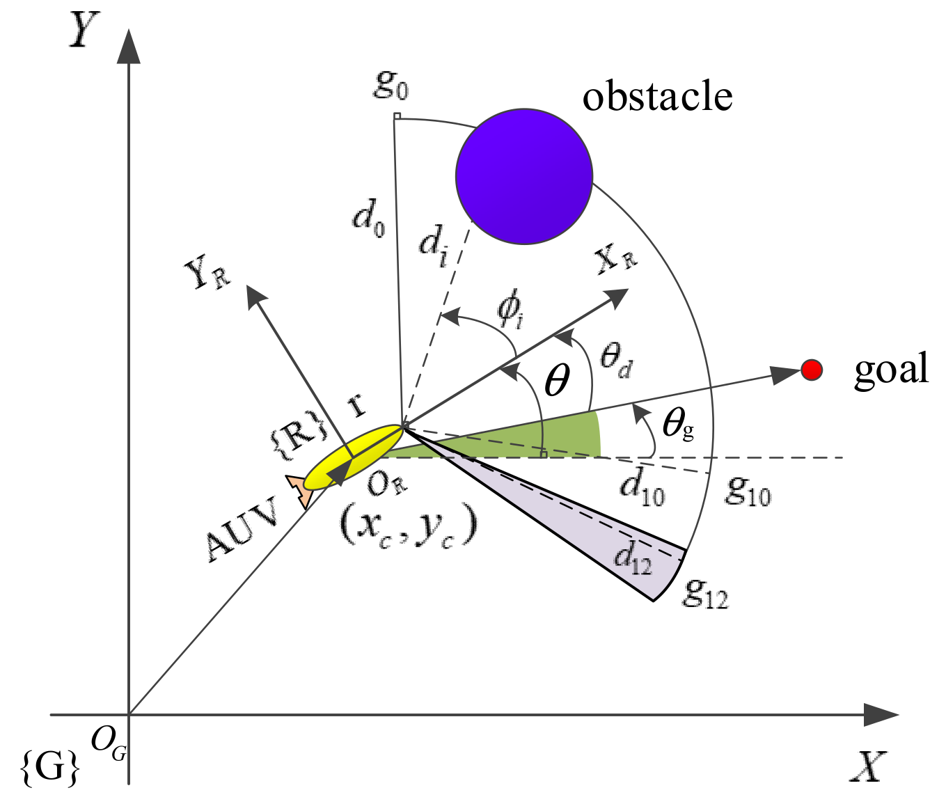
A moving AUV may encounter static and dynamic obstacles during navigation. In this paper, the state information of the external environment is assumed to be mainly obtained by an active sonar sensor. Consider 256 beams divided into 13 groups ${\{\mathrm{g}}_0{,\mathrm{g}}_1{,\mathrm{g}}_2,\dots \dots {\mathrm{g}}_{11}{,\mathrm{g}}_{12}\}$, with ${\{\mathrm{g}}_1{,\mathrm{g}}_2,\dots \dots {\mathrm{g}}_{11}\}$ consisting of 20 beams and ${\mathrm{g}}_0,{\mathrm{g}}_{12}$ including 18 beams. These beams are used to judge whether there is an obstacle around the AUV and whether there is an optimal path for the AUV that does collide with the obstacle. Assume that the X-axis of the AUV coordinate system {R} is consistent with the moving direction and that the positive Y-axis points outward from the left side of the AUV. As shown in Figure 1, $d_i$ represents the minimum distance from the obstacle detected by the $i\mathrm{th}$ group and ${\varphi }_i$ is the angle corresponding to the minimum distance. The coordinates of the obstacle in the global coordinate frame {G} can be expressed as:

$$\left[\begin{array}{c}x\\ y\end{array}\right]=\left[\begin{array}{cc}\cos \theta & -\sin \theta \\ \sin \theta & \cos \theta \end{array}\right]\left[\begin{array}{c}{d}_i\cos {\varphi }_i+\mathrm{r}\\ d_i\sin {\varphi }_i\end{array}\right]+\left[\begin{array}{c}{x}_c\\ y_c\end{array}\right]$$

(1)

where $(x,y)$ are the coordinates of the obstacle in the global coordinate frame {G}, $\mathrm{r}$ is the distance from the sonar to the center of mass of the AUV, $\theta$ is the angle between the X-axis of the coordinate frames {R}and{G}, ${\theta }_{\mathrm{g}}$ is the angle between the AUV and the target point relative to the X-axis $({\theta }_d={\theta }_g-\theta )$, with positive values running counterclockwise, and $(x_c,y_c)$ is the current position of the AUV in {G}.

2.2. AUV Model

In this paper, we consider only the three horizontal degrees of freedom (DOFs) when designing the guidance system for the AUV. The 3-DOF kinetics and dynamics can be represented as:

$$\dot{\mathsf{\eta }}=R\left(\theta \right)\mathsf{\nu }$$

(2)

$$M\dot{\mathsf{\nu }}+C(\mathsf{\nu })\mathsf{\nu }+D(\mathsf{\nu })\mathsf{\nu }=\mathsf{\tau }+\stackrel{⌢}{\mathsf{\tau }}$$

(3)

In this article, the AUV movement process does not consider the interference of wind, waves, and currents. This matrix shows properties of: $R{(\theta )}^{T}R(\theta )=I$.

The 3-DOF kinematics can be simplified to:

$$\left\{\begin{array}{c}\dot{x}=u\cos \theta -v\sin \theta \\ \dot{y}=u\sin \theta -v\cos \theta \\ \dot{\theta }=r\end{array}\right.$$

(4)

The 3-DOF dynamics can be represented as:

$$\left\{\begin{array}{l}\dot{u}=(-d_{u}u+{\tau }_u)/m_u\hfill \\ \dot{v}=(C_1{m}_r+C_2{Y}_{\dot{r}})/(m_v{m}_r-Y_{\dot{r}}^2)\hfill \\ \dot{r}=(C_2{m}_v+C_2{Y}_{\dot{r}})/(m_v{m}_r-Y_{\dot{r}}^2)\hfill \end{array}\right.$$

(5)

$C_1=-d_{v}v+(Y_r-m_{u}u)r$, $C_2=(N_v-m_{uv}u)v-d_{r}r+{\tau }_r$, $m_u=m-X_{\dot{u}}$, $m_v=m-Y_{\dot{v}}$, $m_r=I_z-N_{\dot{r}}$, $m_{uv}=X_{\dot{u}}-Y_{\dot{v}}$, $d_u=Y_v+Y_{\left|v\right|v}\left|v\right|$, $d_r=N_r+N_{\left|r\right|r}\left|r\right|$, $m=40\mathrm{kg}$, $I_z=8.0\mathrm{N}\cdot {\mathrm{m}}^2$. The AUV model parameters are listed in

Table 1. The parameters of the AUV model.

$X_{\dot{u}}$	$X_{u_r}$	$X_{\left|u\right|u}$	$Y_{\dot{r}}$	$Y_{\dot{v}}$	$Y_r$
$\begin{array}{c}-1.42\\ \mathrm{kg}\end{array}$	$\begin{array}{c}0.1\\ \mathrm{kg}\end{array}$	$\begin{array}{c}8.2\\ \mathrm{kg}\cdot {\mathrm{m}}^{-1}\end{array}$	$\begin{array}{c}-2.5\\ \mathrm{N}\cdot {\mathrm{m}}^2\end{array}$	$\begin{array}{c}-38.4\\ \mathrm{kg}\end{array}$	$\begin{array}{c}5\\ \mathrm{kg}\end{array}$
$Y_{ur}$	$Y_{\left|v\right|v}$	$N_v$	$N_{\dot{v}}$	$N_r$	$N_{\left|r\right|r}$
$\begin{array}{c}0\\ \mathrm{kg}\cdot {\mathrm{m}}^{-1}\end{array}$	$\begin{array}{c}200\\ \mathrm{kg}\cdot {\mathrm{m}}^{-1}\end{array}$	$\begin{array}{c}36\\ \mathrm{kg}\end{array}$	$\begin{array}{c}2.2\\ \mathrm{kg}\end{array}$	$\begin{array}{c}5\\ \mathrm{kg}\cdot \mathrm{m}\end{array}$	$\begin{array}{c}15\\ \mathrm{kg}\end{array}$

.

2.3. The Line-of-Sight Guidance System

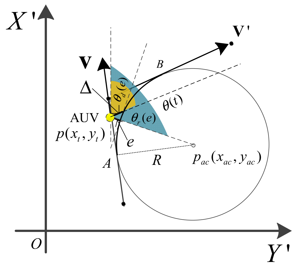
The planning algorithm in this paper is realized by adjusting the heading of the AUV. When the planning policy is $h_0$ at time $t$, then the heading of the AUV at time $t+1$ will increase by ${10}^o$, which is impossible in practical applications. With such a large change in an instant, the AUV heading can only be adjusted gradually through control. To make the trajectory smoother and achieve precise tracking control, a line-of-sight [30] method is used to solve this problem. As seen from Figure 2, assuming that the angle between the velocity $V$ at time $t$ and the velocity $V’$ at time $t+1$ is ${10}^o$ to show more clearly, the angle in Figure 2 is not ${10}^o$, we choose a forward-looking vector $\Delta$ as the reference for trajectory tracking to obtain the desired error angle ${\theta }_d(e)$ (where ${\theta }_d(e)$ is the achievable target of the propeller and rudder). By continuously calculating ${\theta }_d(e)$, the AUV is slowly transferred from point A to point B. The following experiments also show that the guidance algorithms can cause the AUV to perfectly track the required trajectory.

A careful inspection of Figure 2 gives the following formulas:

$$\theta (t)=\frac{\pi }{2}+\arctan (\frac{x(t)-x_{ac}}{y(t)-y_{ac}})$$

(6)

The tracking error is:

$$e={‖p_{ac}-p‖}_2-R$$

(7)

$${\theta }_{\mathrm{d}}(e)=\theta (t)-{\theta }_r(e)=\left\{\begin{array}{c}\theta (t)-\arccos (\frac{\left|e\right|}{{‖\Delta ‖}_2}),\left|e\right|\le {‖\Delta ‖}_2\\ {\theta }_t(t)-\frac{\pi }{2},\mathrm{else}\end{array}\right.$$

(8)

where $p(x_t,y_t)$ represents the current position of the AUV and $p_{ac}(x_{a\mathrm{c}},y_{ac})$ represents the center position of the transition arc. ${\theta }_r(e)$ is the angle between the forward-looking vector $\Delta$ and the vector $\overrightarrow{p{p}_c}$, where $\Delta$ is the forward view vector parallel to the next desired trajectory. ${\theta }_d(e)$ represents the desired angle, and $\theta (t)$ is the angle between the vector $\overrightarrow{p{p}_{ac}}$ and the $X’$-axis. The coordinate system $X’OY’$ in Figure 2 is not related to the $XOY$ in Figure 1.

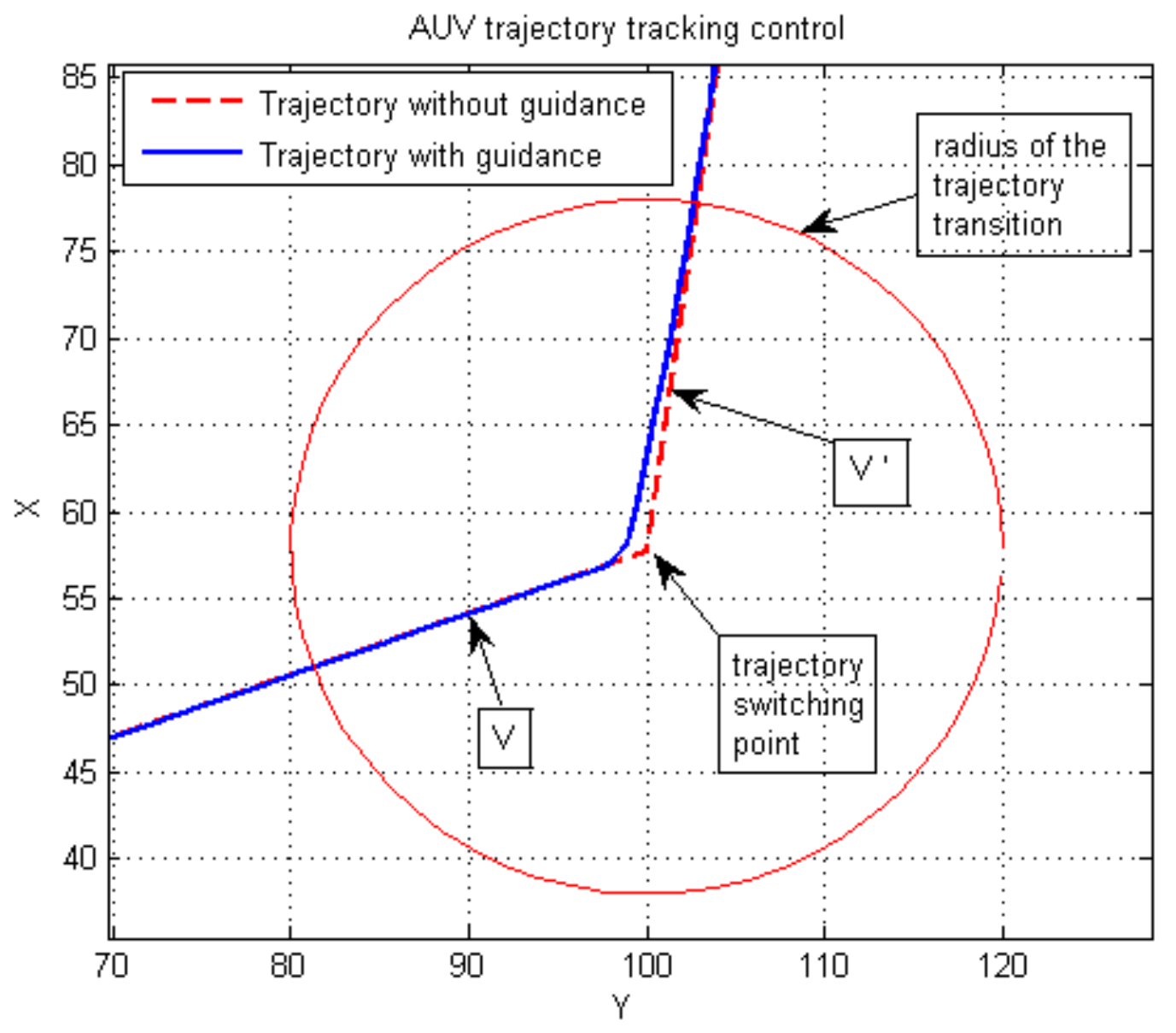
Figure 3 verifies the effect of the line-of-sight guidance algorithm. The AUV adopts a new steering strategy at the trajectory transition point and the velocity changes from $V$ to $V’$. The heading of the AUV has to be adjusted to a large degree, which is difficult to accomplish if it only relies on the propeller and rudder. The red dotted line represents the trajectory without the guidance algorithm, and the solid blue line represents the trajectory with the guidance added. The red circle represents the radius of the trajectory transition. After introducing this guidance algorithm, the trajectory changes slowly, rather than sharply, near the trajectory switching point, instead of violently changing. The red circles represent the process of track switching.

3. Proposed Deep Reinforcement Learning Algorithm

When using RL to solve robotic control problems, we assume that the robot’s environmental model is a finite Markov decision process (MDP). In addition, the whole environment is fully observable. The path planning task considers the results of the AUV’s interaction with the environment through a series of actions in discrete time steps.

We assume that the information received by the AUV from the active sonar is $D_t\subseteq \{d_{0t},d_{1t}\cdots d_{it}\cdots d_{12t}\}$$(i=0,1,2,\dots \dots 12)$ at time $t$. We assume that the AUV receives observations $D_t$ of the simulation environment $E$, $D_t\subset {ℝ}^{13}$, and then the agent selects a heading adjustment $h_t$. The AUV receives a numerical reward $r_{t+1}\in ℝ$ and transfers to the next state according to the probability $p(D_{t+1},r_{t+1}|D_t,h_t)$, where $p$ is the probability distribution for each state $D_t$ and choice $h_t$.

The expected reward $r_{t+1}$ for state-action pair $(D_t,h_t)$ is computed as:

$$r_{t+1}\triangleq r(s_t,a_t)={\rm E}[R_{t+1}|D_t,h_t]={\displaystyle \sum _{r_{t+1}\in ℝ}{r}_{t+1}}{\displaystyle \sum _{s_t\in S}p(D_{t+1},h_{t+1}|D_t,h_t)}$$

(9)

The aim is to select the heading adjustment $h_t$ that maximizes the expected value of the cumulative sum of the received scalar signals. The optimal action-value function $Q^{*}(D,h)$ defines the maximum expected return for heading adjustment $h$ in state $D$ and the decisions thereafter, following an optimal policy.

$$Q^{*}(D,h)={\max }_{\pi }E[{\displaystyle {\sum }_{t’=t}^T{\gamma }^{t’-t}{r}^{t’}|D_t=D,h_t=h,\pi }]$$

(10)

where policy $\pi (h|D)$ is the probability of selecting action $h_t=h$ when $D_t=D$, $T$ is the termination time-step of the episode, $\gamma$ is a discount rate and $0\le \gamma \le 1$.

The optimal action-value function $Q^{*}(D,h)$ obeys an important identity known as the Bellman equation [31]

$$Q^{*}(D,h)=E[r_{t+1}+\gamma \underset{a_{t+1}}{\max }{Q}^{*}(D_{t+1},h_{t+1})|D_t=D,h_t=h]$$

(11)

Watkins and Dayan proved that $Q^{\pi }(D_t,h_t)\to Q^{*}(D,h)$ with a probability of 1 as $t\to \infty$ [31].

When actually applying the Q-learning algorithm, we allow $t$ to be sufficiently large to approximate the action value $Q(D,h)$. Sometimes we also use linear or nonlinear NNs with weights $w$ as a Q-network to estimate the action-value $Q(D,h;w)\approx Q^{*}(D,h)$. Nonlinear NNs diverge in many cases, but they are often successfully used. In this paper, we use an off-policy technique to solve the challenges of exploration and exploitation.

The Q-network can be trained by minimizing the loss function $L_t(w_t)$:

$$L_t(w_t)=E_{D,h\sim \rho }[{(y_t-\widehat{Q}(D_t,h_t;w_t))}^2]$$

(12)

where $y_t=E_{D_{t+1}\sim \xi }[r_{t+1}+\gamma \underset{h_{t+1}}{\max }Q(D_{t+1},h_{t+1};w_{t-1})|D_t,h_t]$ is the target value for iteration $t$, and $\rho$, $\xi$ describes the behavior distributions when the AUV receives observations $D_t$ and makes heading adjustments $h_t$, and $\widehat{Q}(D_t,h_t;w_t)$ is the estimated value of the NN’s network output. Differentiating the loss function $L_t(w_t)$ with respect to the weight $w_t$, the following gradient is obtained:

$${\nabla }_{w_t}{L}_t(w_t)=E[(r_{t+1}+\gamma \underset{h_{t+1}}{\max }Q(D_{t+1},h_{t+1};w_{t-1})-\widehat{Q}(D_t,h_t;w_t)){\nabla }_{w_t}\widehat{Q}(D_t,h_t;w_t)]$$

(13)

The weight $w_t$ is updated according to:

$$w_{t+1}=w_t+\alpha {\nabla }_{w_t}{L}_t(w_t)$$

(14)

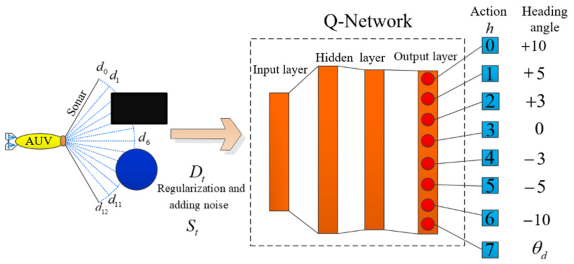
The stability and convergence of DRL must be considered [32] when using a nonlinear function approximator. Instabilities may result from small updates to $Q(D,h)$, and these may significantly change the policy, the correlations present in the sequence of observations, and the correlations between the action-values and the target values [18]. We use a biologically inspired mechanism termed “experience replay” and adjust the action values toward the target values through periodic updates. To train the network, we process the data $D_t\subseteq \{d_{0t},d_{1t}\cdots d_{it}\cdots d_{12t}\}$$(i=0,1,2,\dots \dots 12)$ measured by the active sonar through regularization and noise processing to obtain the input state of the network [33]. Each neuron in the output layer corresponds to the Q-value.

The meaning of each action $h$ is defined in Figure 4; each action corresponds to a heading change angle, with positive values representing $\theta$ increasing, negative values representing $\theta$ decreasing, 0 representing no change, and neuron 7 representing the agents causing the algorithm to search blindly in the environment for a long time. The advantage of using neuron 7 is that the DQN algorithm has the ability to find a target point in some way; thus, we can reduce the time spent in an invalid search environment and increase the probability of reaching the target point.

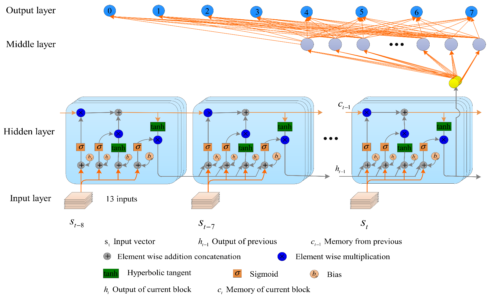
AUV collision avoidance planning is essentially a matter of making decisions based on the state of sequential observations [34]. LSTM has proven to provide state-of-the-art performance in many sequence prediction problems. In the process of learning, the overestimation that occurs when a nonlinear network is used to approximate the Q-value seriously affects the performance of the algorithm. The D-DQN approach can be used to reduce overestimation, making the algorithm more stable and enabling reliable learning. Inspired by the literature [18], we use D-DQN, and the Q-network uses LSTM to build a new algorithm called double DQN-LSTM(D-DQN-LSTM). The structure of the Q-network in the D-DQN-LSTM algorithm is shown in Figure 5, where the output layer neurons have the same meaning as in Figure 4.

The target value $y_t^{DQ}$ used by D-DQN-LSTM is then:

$$y_t^{DQ}=E_{D_{t+1}\sim \xi }[r_{t+1}+\gamma Q(D_{t+1},\underset{h}{\arg \max }\widehat{Q}(D_{t+1},h;w_t);w_t{}^{’})]$$

(15)

Similarly to Expression (13), the update amount of the weight $w_t$ is updated according to:

$${\nabla }_{w_t}{L}_t(w_t)=E[(r_{t+1}+\gamma Q(D_{t+1},\underset{h}{\arg \max }\widehat{Q}(D_{t+1},h;w_t);w_t{}^{’})-\widehat{Q}(D_t,h_t;w_t)){\nabla }_{w_t}\widehat{Q}(D_t,h_t;w_t)]$$

(16)

The concept of using reward signals to form goals is one of the most distinctive features of RL. The AUV’s goal is to maximize the total amount of reward it receives while avoiding obstacles and reaching the target point in the process of motion. The reward function is:

$$r_t=\left\{\begin{array}{cc}-3& d_i\le 1\\ -0.5& 1<d_i<5\\ 5& \mathrm{reach}\mathrm{target}\mathrm{point}\\ 0& \mathrm{other}\mathrm{else}\end{array}\right.$$

(17)

where $d_i$ indicates the distance between the AUV and the obstacle. $d_i\le 1$ indicates that the AUV has encountered an obstacle, and $1<d_i<5$ indicates that the AUV is too close to the obstacle, which means that the AUV does not have enough time to adjust the heading to avoid obstacles. If the AUV reaches the target point, it receives a positive reward value. In the other situations, the reward value is 0.

The pseudo-code of the algorithm is as follows:

Algorithm DQN-LSTM algorithm with experience replay for the AUV

Input: the linear velocities $\varpi =[u,v,r]$, the position vector $\eta =[x,y,\theta ]$, and the sonar information $D$.

Initialize the environment E.

Initialize replay memory M to capacity N.

Initialize the $Q$-networks and the target $\widehat{Q}$-networks with random weights.

for episode = 1, $K$ do

Initialize sequence $D_1$ and preprocess sequencing $S_1=\psi (D_1)$.

for $t=1,T$ do

With probability $\epsilon$ select a random action $h_t$

otherwise select $h_t={\max }_h{Q}^{*}(\psi (D_t),h;w)$.

Execute action $h_t$ in emulator: put $\varpi ,\eta ,h_t$ into the AUV model.

update the environment E and get the state $D_{t+1},r_{t+1}$.

Store transition $(\psi (D_t,h_t,r_t,D_{t+1}))$ in M.

Store transition $(\psi (D_t,h_t,r_t,D_{t+1}))$ in M.

Sample random minibatch 64 of transitions $(\psi (D_j,h_j,r_j,D_{j+1}))$ from M.

Set $y_j=\left\{\begin{array}{c}{r}_j\\ r_j+\gamma {\max }_{h^{’}}Q(\psi (D_{t+1},h^{’};w))\end{array}\right.\begin{array}{c}for\mathrm{terminal}\mathrm{state}\\ for\mathrm{non}-\mathrm{ternimal}\mathrm{state}\end{array}$

Perform a gradient descent step on ${(y_j-Q(\psi (D_j),h_j;w))}^2$ according to Equation (13).

Reset the target $\widehat{Q}$-Networks $\widehat{Q}=Q$ every 50 steps.

end for

end for

4. Simulation Experiment and Discussion

Extensive simulation studies were conducted to demonstrate the effectiveness of the newly proposed method. We used PyGame to draw the interface, AUV, and obstacles, and other entity attributes were drawn using the Pymunk library, while the network structure of the algorithm was the calling Keras library, and the programming language was Python. The results produced by the different scenarios were used to evaluate the performance of the methods under different conditions. We evaluated various network structures to determine the optimal collision avoidance planning algorithm.

4.1. Experimental Detail

The DQN algorithms were trained on a computer with an Intel i5 processor using four CPU cores and a GTX 960 M. The parameters of the Q-network, using a fully connected network and LSTM, were basically the same during the training process. We used the Adagrad optimizer with a learning rate of $\alpha ={10}^{-4}$ to learn the network parameters. The hidden layer activation functions of the network were the leaky ReLU, tanh, and sigmoid functions. The activation function of the output layer used a tanh activation function, which defines the range of the action-value function. To improve the robustness and stability of the network model, the following tricks were used in the training process: (1) Gaussian noise was added to the input of the network, and (2) dropout (ratio of 0.2) was applied to each hidden layer. We used different numbers of hidden layer units $[[30,40],[164,150],[256,256],[512,512]]$, minibatch sizes of 64, and experience buffer sizes of 50,000 to verify the planning capability of the models.

The parameters used in the training phase of DRL: gamma = 0.9, number of frames to observe before training (observe = 1000), epsilon = 0.95, training_frames = 500,000, lstm_network_weights = [−0.5, 0.5], nn_network_weights = [−1, 1].

We can see from

Table 2. Comparison of the results of different algorithm training.

	Number of Neurons in the Hidden Layer	Model Training Time(h)	Convergence Step	Convergence Accuracy
DQN	[30,40]	2.4	3797	0.089 ~ 0.092
	[164,150]	2.9	6492	0.085 ~ 0.091
	[256,256]	3.7	8045	0.093 ~ 0.096
	[512,512]	4.9	6263	0.092 ~ 0.097
DQN-LSTM	[30,40]	6.8	3095	(7.15 ~ 7.75) × 10−5
	[164,150]	9.6	5509	(1.05 ~ 1.13) × 10−5
	[256,256]	10.5	5908	(3.43 ~ 3.57) × 10−5
	[512,512]	11.2	4103	(1.10 ~ 1.16) × 10−5
D-DQN	[30,40]	2.6	3548	0.087 ~ 0.093
	[164,150]	3.3	4126	0.090 ~ 0.095
	[256,256]	4.2	6237	0.076 ~ 0.080
	[512,512]	5.1	3877	0.073 ~ 0.076
D-DQN-LSTM	[30,40]	9.1	3124	(4.48~ 4.78) × 10−5
	[164,150]	11.3	3504	(3.15 ~ 3.37) × 10−5
	[256,256]	12.4	5307	(1.49 ~ 1.62) × 10−5
	[512,512]	13.7	3440	(5.88 ~ 6.11) × 10−5

that the DQN model has the shortest training time required for different models. As the number of neurons in the hidden layer increases, the time required to train each model also increases. The $[256,256]$ model gives the slowest convergence of the loss function converges, whereas the $[30,40]$ model gives the fastest convergence. The disadvantage of this early convergence is that the algorithm cannot effectively search the entire environment, and some optimal strategies may not be identified. The $[164,150]$ model is the smallest of all structures to achieve reasonable convergence accuracy. The converged value of the loss function convergence value using the LSTM network is much smaller than that given by NN, regardless of whether the DQN algorithm or the D-DQN algorithm is used. As D-DQN has one more target network than DQN, the weights must be updated at certain intervals, so a longer training time is required. The same phenomenon occurs for the DQN-LSTM and D-DQN-LSTM models. Considering these various factors, a network structure with 164 units in the hidden layer and 150 in the middle layer is considered optimal.

4.2. Testing the Performance of the Algorithm

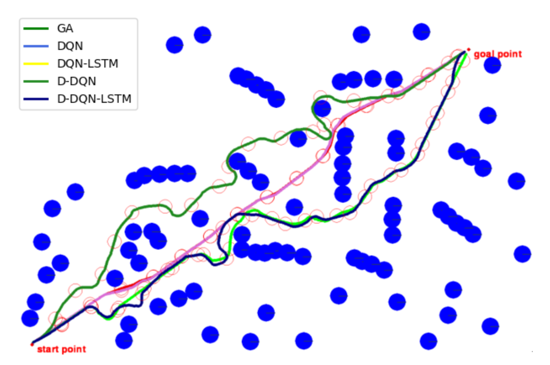
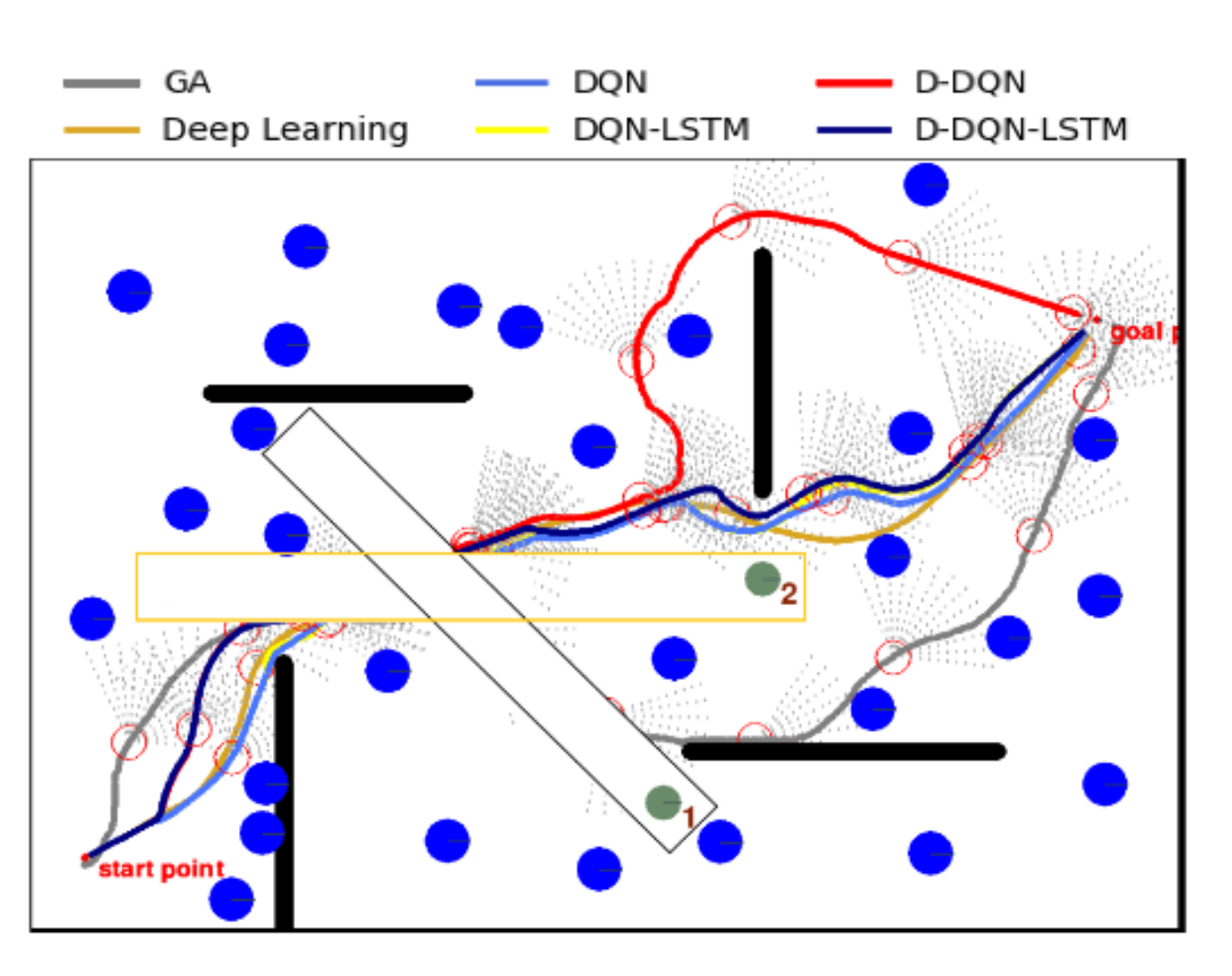
To evaluate the collision avoidance planning capabilities of the various above algorithms, we compared them in different test environments, including static obstacles, mixed obstacles, and complex dynamic obstacles. The obstacles, start point, and endpoint positions were randomly generated in the test environment, and the GA algorithm results were used as the benchmark for comparison. During training, the environment contained only circular obstacles with a radius of 25. To test the performance of the algorithms, a variety of obstacles were added to the test environment, which did not appear in the training environment. In Test 1, the advantages of adding policy 7 were verified, and the stability of the 5 methods was also tested. In Test 2, the collision avoidance planning performance of the 5 algorithms was compared in a static environment. In Test 3, dynamic obstacles and a deep learning algorithm were added, and the collision avoidance planning performance of the 6 algorithms was compared. In the trajectory figure of the test, the hollow circle represents the safety distance of the AUV, the solid blue circle, the blue square, and the black rectangle represent the static obstacles, and the dark sea-green solid circles represent the dynamic obstacles.

4.2.1. Test 1

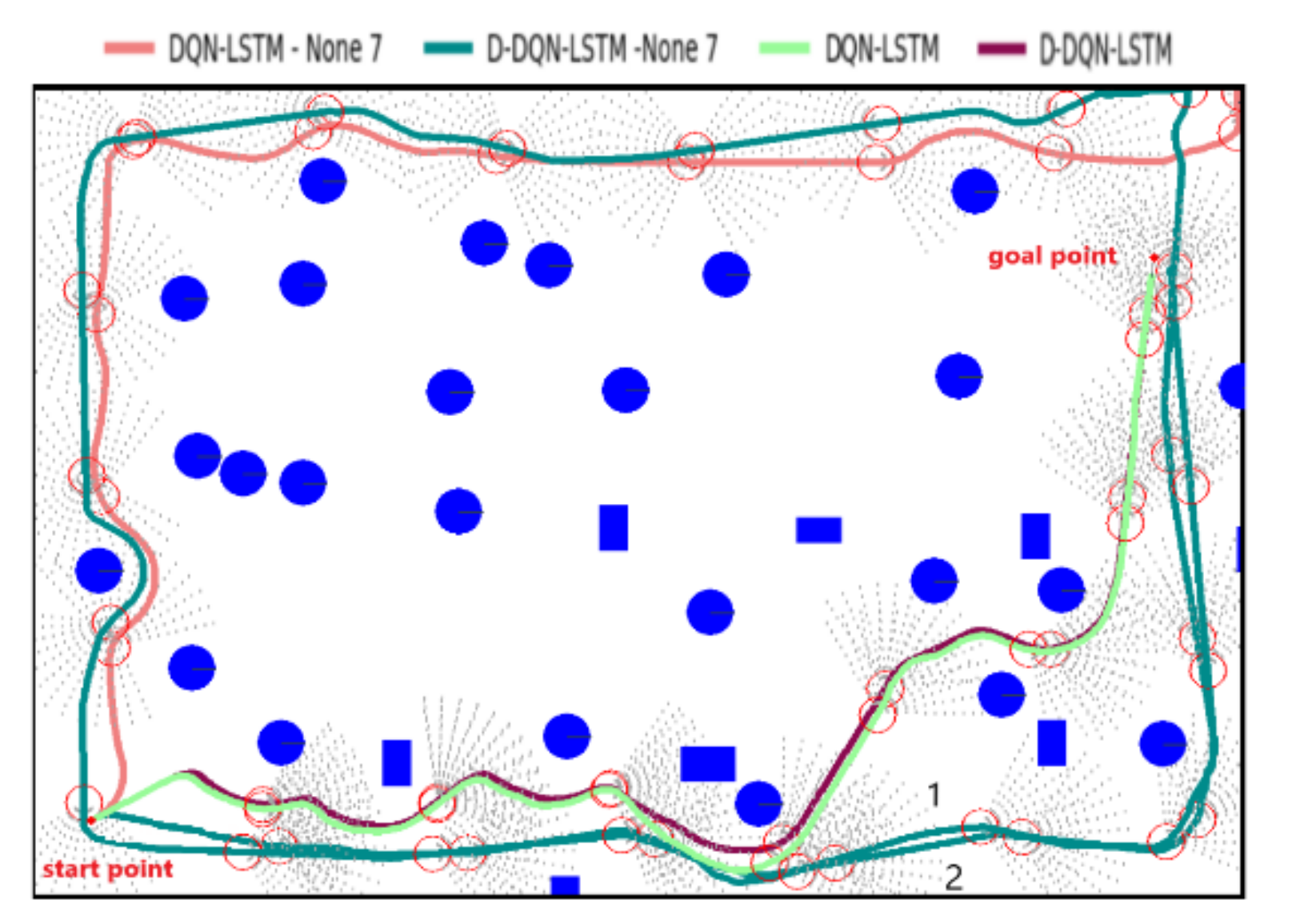
To verify the advantages of adding policy 7, the network model was retrained for the DQN-LSTM and D-DQN-LSTM algorithms without policy 7. Figure 6 shows the planned trajectories of the 4 algorithms in the test environment. Figure 6 shows that DQN-LSTM-None 7 cannot find the goal point. When D-DQN-LSTM-None 7 first arrived near the goal point, it did not move toward the goal point and then went through another round to arrive at the goal point. In contrast, the 2 algorithms of policy 7 move toward the target point from the beginning, and under the guidance of policy 7, the two algorithms reach the goal faster. Compared with the no policy algorithms, the policy 7 algorithms have the guidance of the goal point. When there are no obstacles around the AUV, the policy of moving to the target point is better than blind search, which can save considerable time in model training. In addition, the lack of a goal point to obtain the maximum reward also affects the accuracy of the model.

Table 3. Comparison of algorithms performance with and without policy 7.

	Convergence Step	Training Time (h)	Success Rate (%)
DQN-LSTM-None 7	$9352$	$13.6$	$37$
D-DQN-LSTM-None 7	$6870$	$18.4$	$46$
DQN-LSTM	$5509$	$9.6$	$91$
D-DQN-LSTM	$3504$	$11.3$	$94$

shows the results of the policy 7 algorithms and the no policy 7 algorithms. The DQN-LSTM and D-DQN-LSTM algorithms have a much higher probability of finding the goal point in the test environment than DQN-LSTM-None 7 and D-DQN-LSTM-None 7. For the former, the number of convergence steps is almost half of the latter, the training time is shorter, and the success rate of reaching the goal point is higher in the test environment. The advantage of adding policy 7 is related to shortening the training time and increasing the probability of reaching the target point.

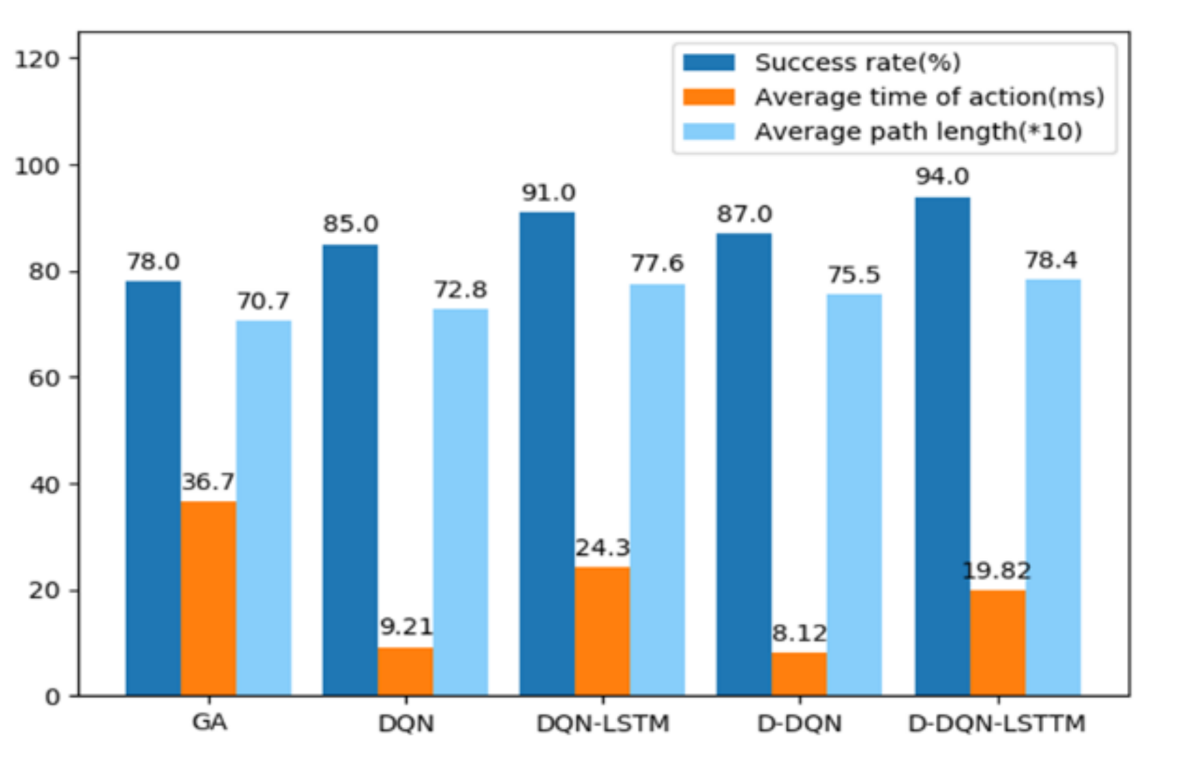
Figure 7 shows that the success rates of the 4 DRL algorithms achieve higher success than the GA. The success rate of the D-DQN-LSTM algorithm has the highest success rate. DQN requires the shortest time to perform an action, whereas D-DQN-LSTM takes the longest time. The GA model is greatly affected by the complexity of the environment, which causes its running time to fluctuate more than that of other algorithms. Because the LSTM network is more complex than the NN, the time required for the DQN-LSTM and D-DQN-LSTM algorithms to perform a single action is longer than the DQN and D-DQN algorithms, and the GA algorithm takes the longest time. The environment changes randomly across 200 episodes. DRL algorithms improve the success rate of AUV reaching the target point, and the execution time of a single action is shorter than the GA algorithm.

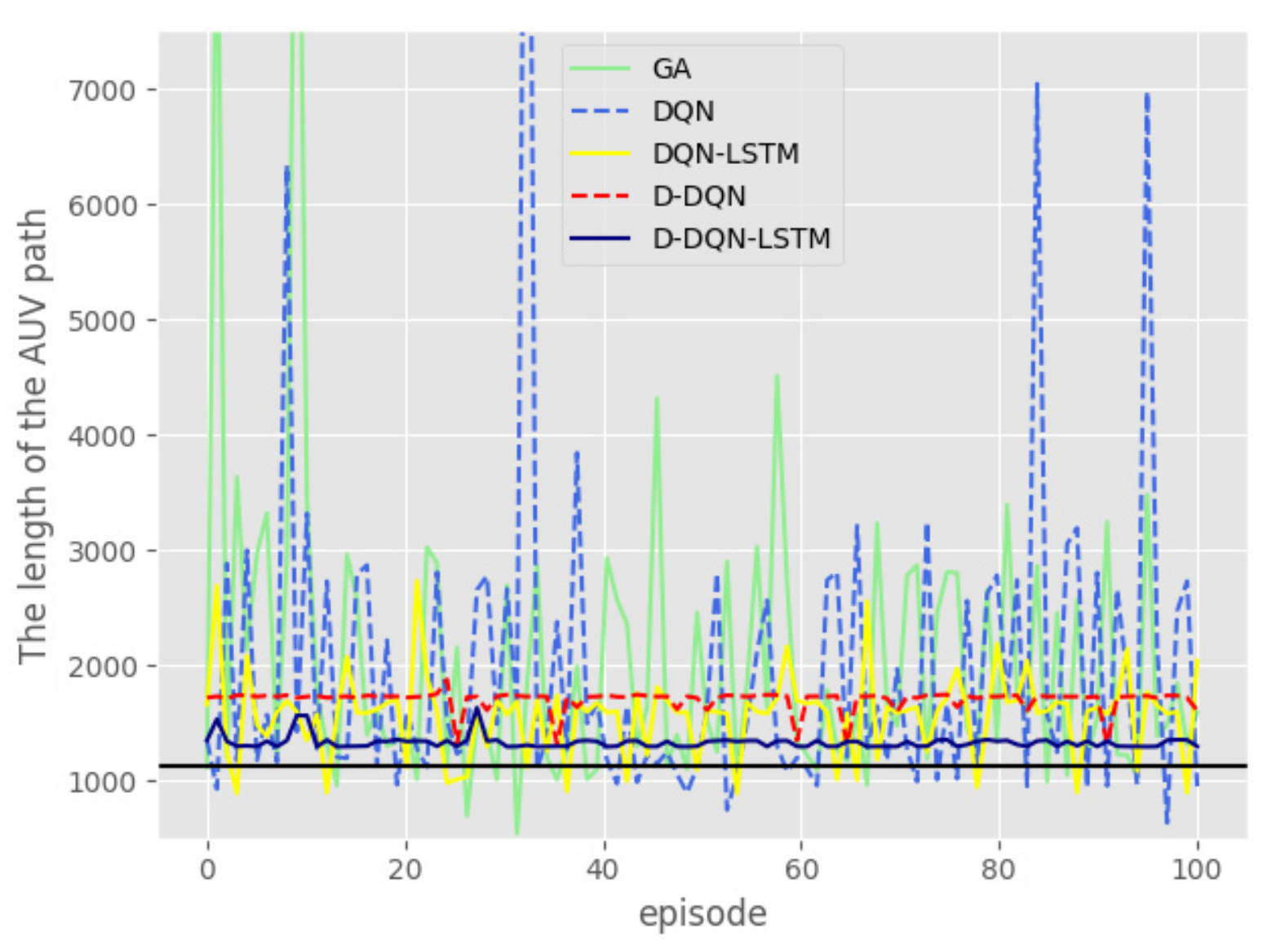
To test the stability of the algorithms in the constant environment, each algorithm was run 100 times to obtain the trajectory, as shown in Figure 8. The path planned by the GA algorithm and the DQN algorithm is tortuous. Figure 8 and Figure 9 show that compared to the other 3 algorithms, D-DQN and D-DQN-LSTM are more stable, and the distance of D-DQN-LSTM is shorter in the 2 optimal algorithms. The path planned by the D-DQN algorithm is very stable, but its path is not optimal. From the above 2 figures, we can conclude that the trajectory planned by the D-DQN-LSTM algorithm is optimal. The black line represents the straight-line distance from the starting point to the goal point.

4.2.2. Test 2

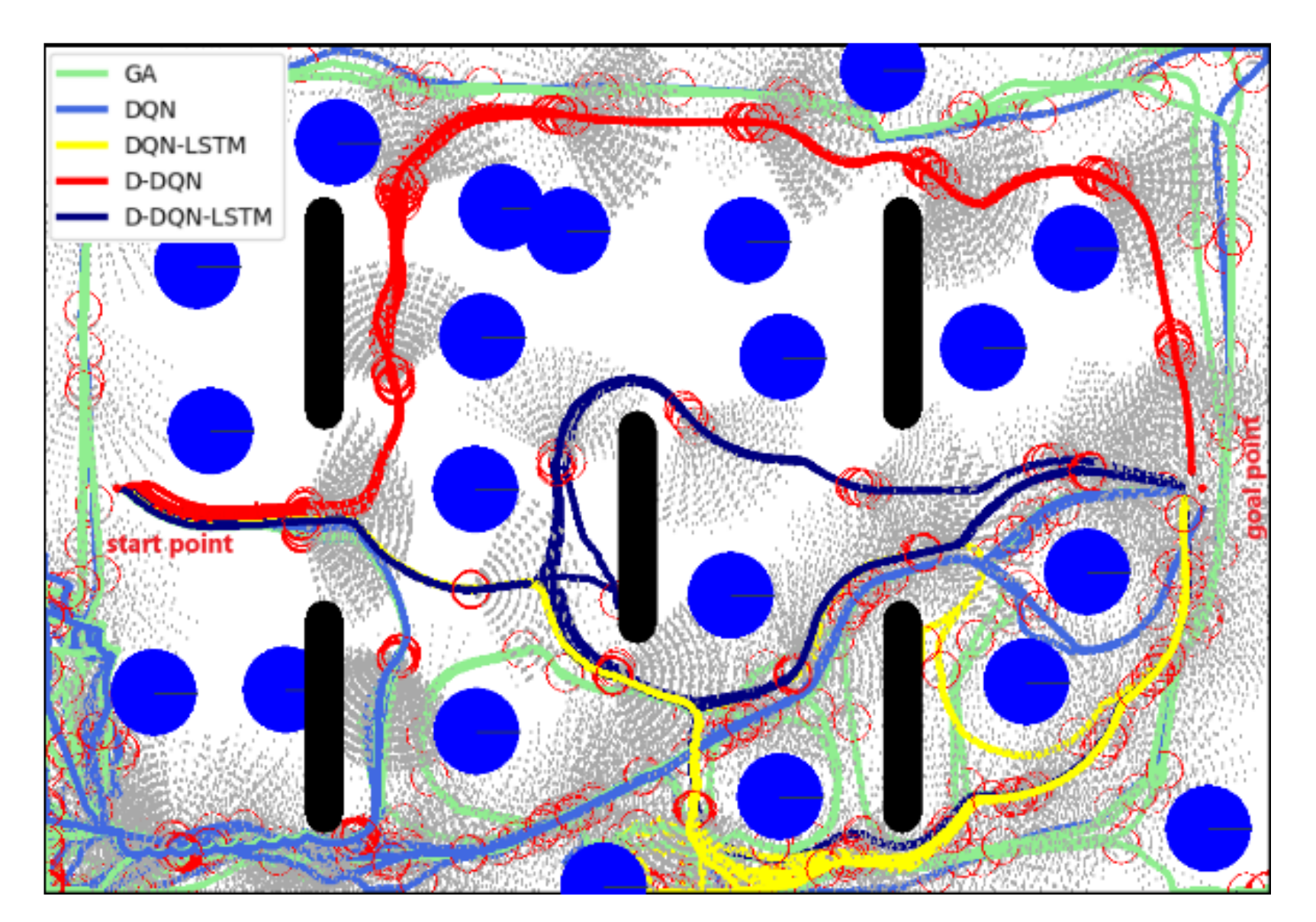
The performances of all 5 methods were tested in a static environment, as shown in Figure 10. GA’s trajectory is covered by DQN. In this test, the speed of the ocean current is 0.25 m/s and the direction is $\frac{\pi }{4}$. Although the path planned by the D-DQN-LSTM algorithm is longer than that of the GA, the path planned by the D-DQN-LSTM algorithm is safe and maintains a certain distance from the obstacles, whereas the path planned by the GA is mostly nearly close to the obstacle boundaries, and there is a danger of collision.

Table 4. Performance comparison of five algorithms in a static environment.

	Number of Actions	Running Time(s)	Path Length(m)
GA	-	$35.81$	$1160$
DQN	$724$	$12.83$	$1162$
DQN-LSTM	$846$	$17.46$	$1360$
D-DQN	$830$	$13.48$	$1351$
D-DQN-LSTM	$892$	$18.37$	$1398$

shows that the path lengths given by the GA model are optimal, and the DQN algorithm is the best of the DRL algorithms. The running times of DQN and D-DQN are faster than those of DQN-LSTM and D-DQN-LSTM. When faced with the same observation value, DQN-LSTM and D-DQN-LSTM output different actions (heading adjustment). Although the path produced by DQN-LSTM basically coincides with that of D-DQN-LSTM, the latter selects a better policy at the critical positions, and the planned path by D-DQN-LSTM gives a more secure path. The D-DQN-LSTM model has the largest number of actions and the longest path, but we can see from Figure 10 that this model produces the safest planned path by D-DQN-LSTM. During the entire movement, the distance between the AUV and all obstacles was more than or equal to the safe distance of 20 m, and no collision occurred. Recall that the security of the AUV is critical in real-world environments.

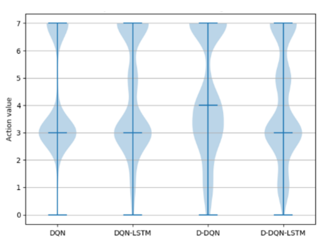
Figure 11 shows the policy distribution of the 4 DRL algorithms. The DQN policy is very simple, focusing on actions 3 and 7, which cause the AUV to continue along the current direction and move toward the target point, respectively. This affects the flexibility and robustness of this algorithm. When encountering a complex environment, the path planning ability will be greatly limited, and the target point will often be missed. From Figure 11, the D-DQN algorithm learns policies 1, 2, 4, 5, and 6 better than the DQN algorithm, ensuring the algorithm’s production of a more uniform and reasonable policy distribution. The same result appears in the D-DQN-LSTM and DQN-LSTM algorithms, with the former policy being more uniform and robust than the latter. This can be verified from Figure 11, where the policy distributions of DQN-LSTM and D-DQN-LSTM are similar, and the generated trajectories are similar to those in Figure 10. The diversification of their policies has the advantage that it demonstrates that these algorithms offer enhanced adaptability and robustness in a given environment.

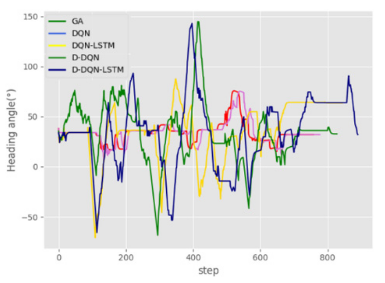
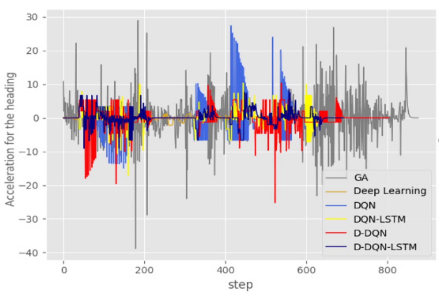
Figure 12 shows that the D-DQN and D-DQN-LSTM algorithms have a larger range of variation, which shows that these algorithms have a stronger ability to explore the environment. This is advantageous in finding the right path in an unknown and complex environment. Figure 13 shows the acceleration curve of the heading angle. It can be seen from the figure that the GA algorithm reaches the maximum acceleration value of $\pm {10}^o$, while the D-DQN-LSTM is basically stable at $\pm 5^o$.

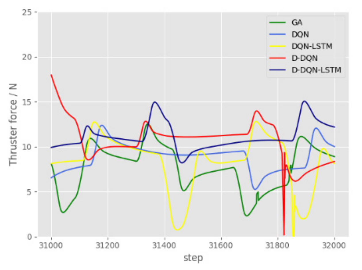
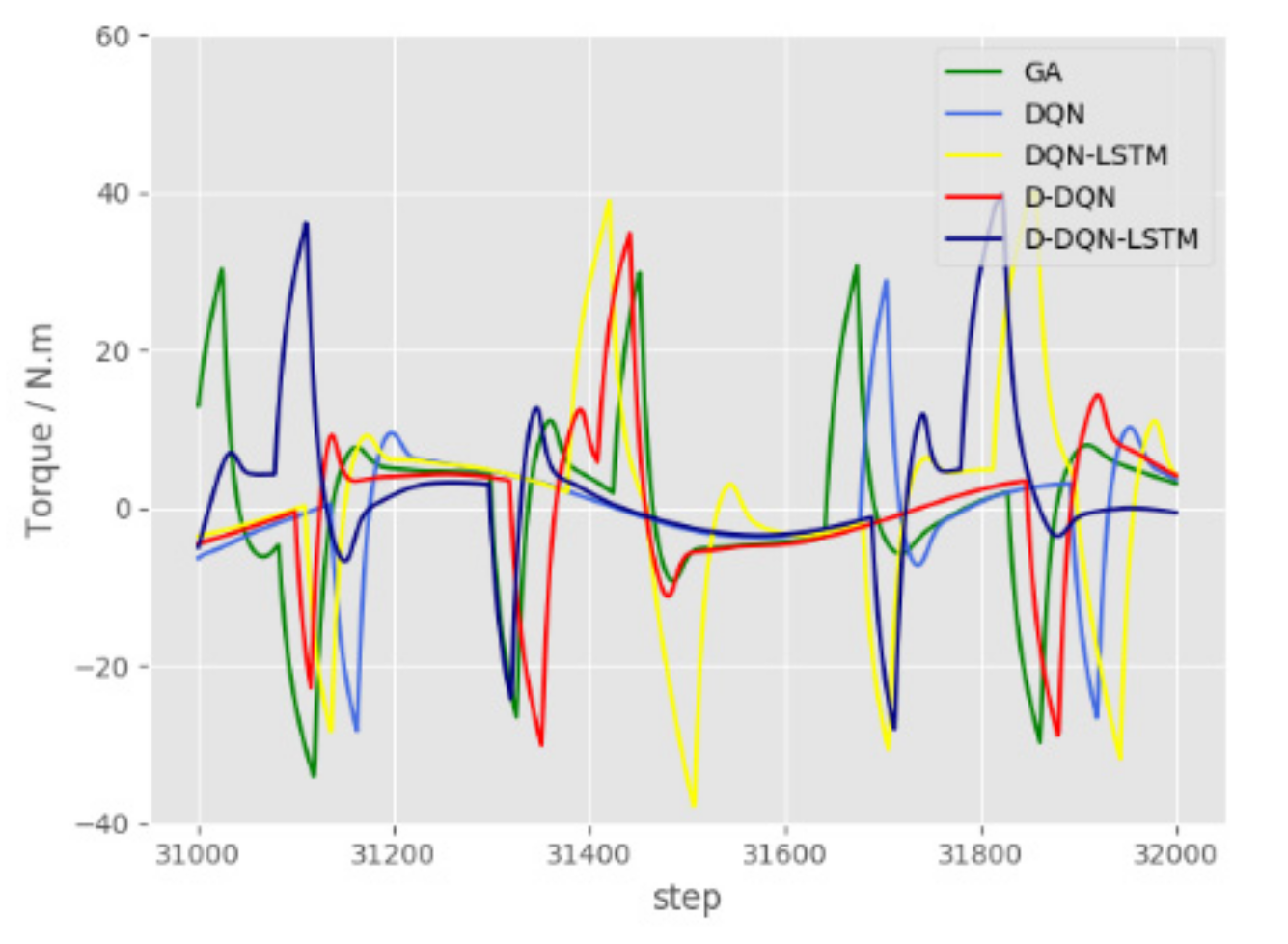
Figure 14 and Figure 15 show that the thrust and moment required by the 5 algorithms to complete the planning under the disturbance of ocean currents in a static environment are between 31,000 and 32,000, and the range of 31,000–32,000 corresponds to 310–320 in Figure 13. In the dynamic model simulation, there are 100 data between two time steps, which causes the horizontal axis to be enlarged by 100 times. The entire presentation will appear chaotic, so only a part of it is displayed. In Figure 14, the fluctuation range of D-DQN-LSTM is smaller than that of GA, D-DQN, D-DQN, and D-DQN-LSTM. The curve is smooth, without jagged and sharp edges. It can be seen from the two sets of partially enlarged pictures that the changing trend of the curve is relatively gentle. In Figure 15, the spikes of DQN and D-DQN-LSTM are also the smallest.

4.2.3. Test 3

Figure 16 illustrates the performance of the algorithms in a complex environment with moving obstacles. The rectangular box in the picture shows the range of the moving obstacles. The AUV trajectory is erased by moving obstacles in the rectangular area. Obstacle 1 moves toward ${135}^o$ at a speed of 10, while obstacle 2 moves horizontally to the left at a speed of 20. In this test, the speed of the ocean current is 0.5 m/s and the direction is $-\frac{\pi }{6}$.

Table 5. Performance comparison of six algorithms in a complicated environment.

	Number of Actions	Running Time(s)	Path Length(m)
GA	-	$45.28$	$1678$
Deep Learning	-	$18.12$	$1388$
DQN	$682$	$10.63$	$1364$
DQN-LSTM	$684$	$17.12$	$1368$
D-DQN	$806$	$11.62$	$1606$
D-DQN-LSTM	$695$	$15.78$	$1352$

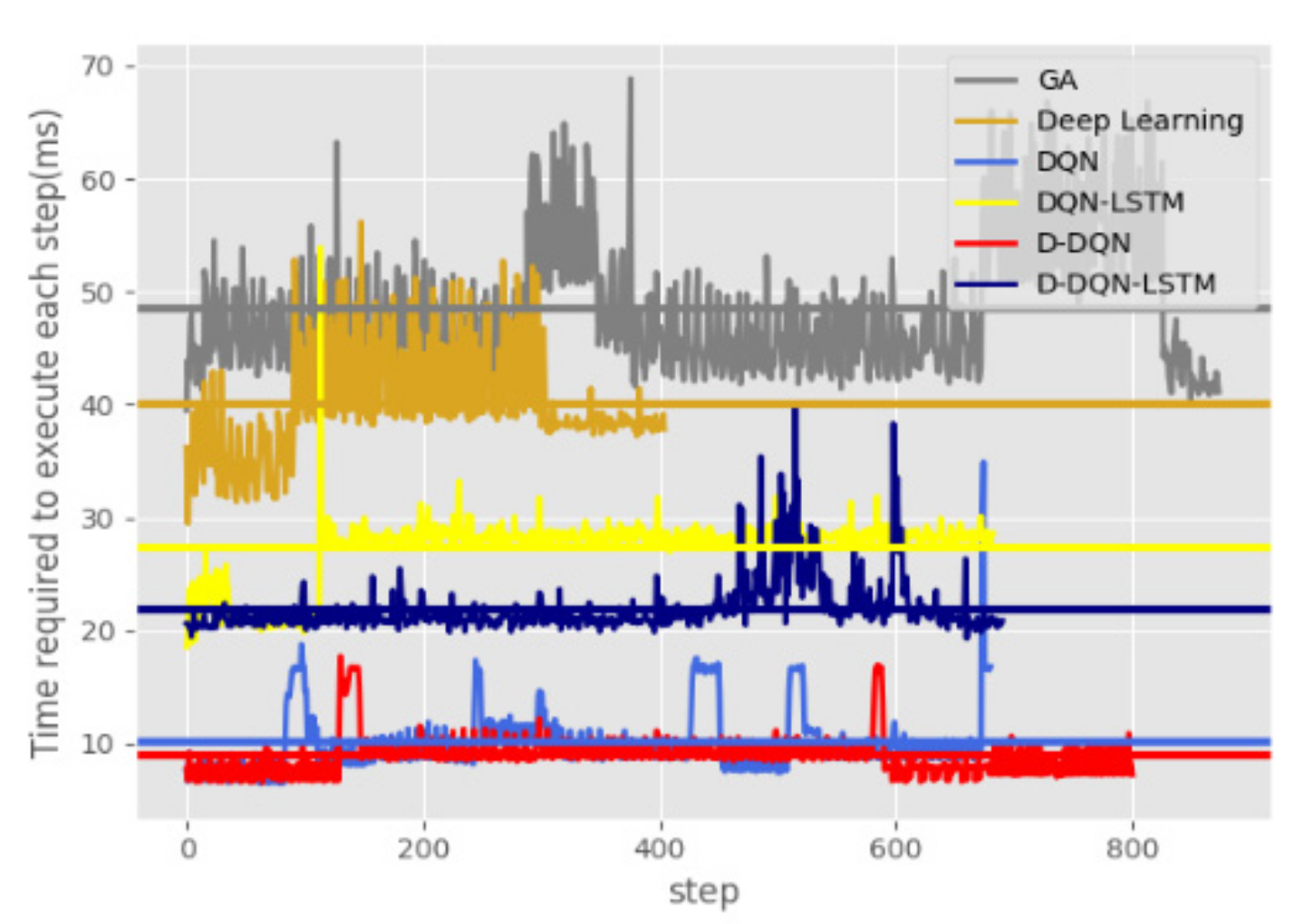
shows the performance indicators of each algorithm. The GA has the longest running time, whereas DQN has the shortest; the longest total path length is produced by the GA algorithm, and while the D-DQN-LSTM algorithm gives the shortest. In terms of the total running time, the DQN-LSTM algorithm is longer than the DQN algorithm, and the same D-DQN-LSTM is also longer than the D-DQN algorithm. This is because the LSTM network is more time-consuming than the NN. It can also be seen from Figure 17 that the curve represents the time required to execute the single-step planning, and where the horizontal line represents the average value. The D-DQN has the shortest average execution time of a single action, while GA has the longest.

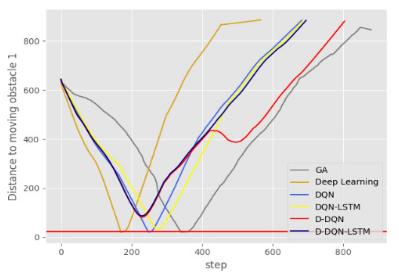
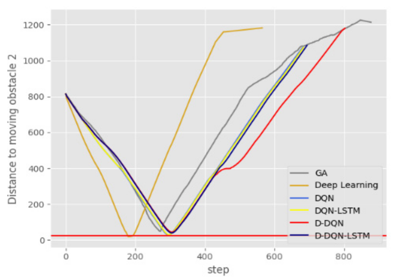
Figure 18 and Figure 19 show the curves of the distance between the AUV and the moving obstacles over time. The horizontal red line in the picture represents a collision between the AUV and the moving obstacle. It can be seen from Figure 18 that neither D-DQN nor D-DQN-LSTM produced a collision with moving obstacle 1. Figure 19 shows that GA, D-DQN, and D-DQN-LSTM did not produce a collision with moving obstacle 2.

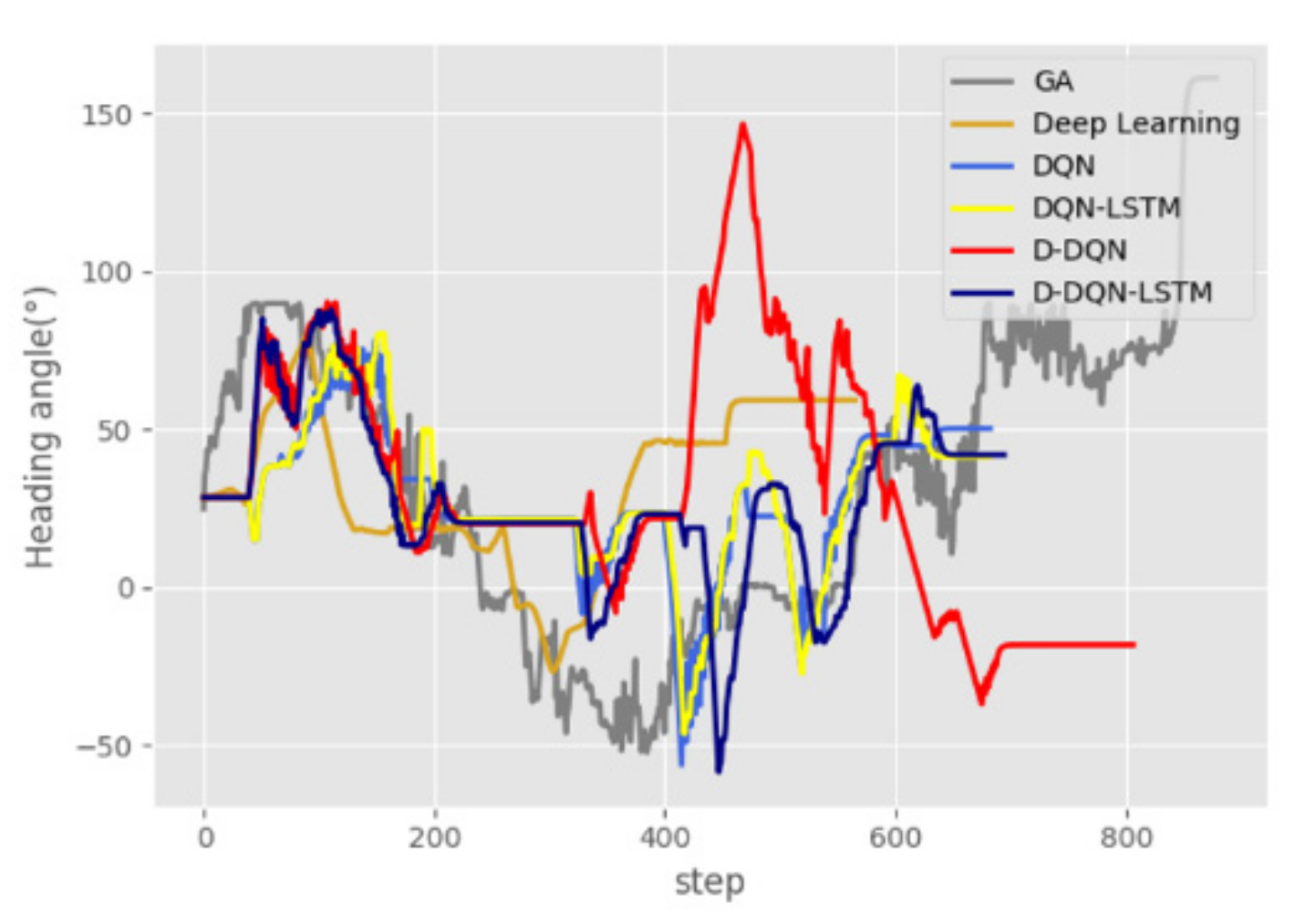
Figure 20 shows the changes in the AUV heading angle. The heading angle change of the GA algorithm is the worst. It can be seen from the figure that the curve of the deep-learning algorithm gives a smoother curve and a smaller fluctuation range. However, this also results in the AUV not having sufficient flexibility to safely avoid dynamic obstacles, especially faster obstacles. D-DQN and D-DQN-LSTM produce large changes in the heading, which makes the AUV more flexible in the environment and provides it with the ability to avoid moving obstacles.

Figure 21 shows the adjustment angle to the heading at each step. The adjustment angle is more frequent in the case of the GA algorithm, and the angle adjusted change in each step is greater than $\pm {20}^o$. This presents a significant challenge to AUV propulsion devices. In terms of heading adjustment, the performance of the four DRL algorithms is worse than that of the DL algorithm. The adjustment angle of the deep learning algorithm produces the smallest angle adjustments, but Figure 16, Figure 18, and Figure 19 show that this model cannot avoid static and dynamic obstacles. D-DQN-LSTM gives the smallest adjustment angles among the four methods proposed in this article, and each adjustment is less than $\pm {10}^o$. This adjustment range is easy to achieve for AUVs.

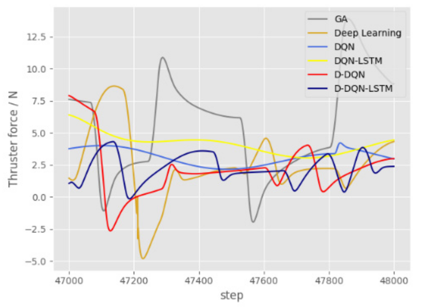
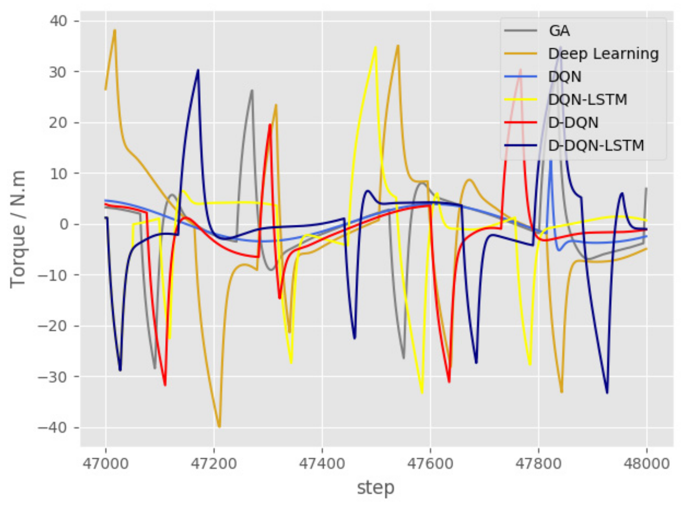
Figure 22 shows the thrust curve of the thruster between 47,000 and 48,000, corresponding to steps 470–480 in Figure 21. Figure 23 shows the corresponding AUV torque curve. Other algorithms require less thrust than GA, and the curve should be smoother. Figure 22 show that the fluctuation amplitude of the force curve of D-DQN-LSTM is smaller than that of other algorithms, which also confirms the curve of heading acceleration in Figure 21.

The negative value of the thrust in Figure 22 is due to the AUV offsetting ocean currents. The function makes the AUV decelerate and makes it easier to turn. The heading of steps 470–480 in Figure 20 is basically maintained at about ${60}^o$, but in Figure 22 and Figure 23, there are fluctuations in thrust and torque, which is due to the response of the AUV to overcome the influence of ocean currents.

4.3. Discussion

To develop collision avoidance algorithms based on deep learning, the first step is to use GA, PSO, random-sample, or other algorithms to collect large numbers of samples, which will greatly reduce the efficiency of algorithm development. In addition, the sample quality and network training performance have a vital impact on the algorithm’s collision avoidance ability. The algorithm proposed in this paper is trained in a simple random environment without the above-mentioned complicated process. After the training is completed, the AUV is placed in a complex dynamic environment and can still effectively avoid collisions. The effectiveness of the algorithm proposed in this paper was verified in two environments: random static and complex dynamic. Simulation experiments have shown that using the approach to the target point as a policy can greatly increase the probability of reaching the target point while also reducing the time required for the algorithm to blindly search the entire environment and improving the efficiency of algorithm learning. The D-DQN-LSTM algorithm is superior in stability and robustness compared to GA and other DRL algorithms. The results show that the D-DQN-LSTM algorithm has significant advantages over other algorithms in terms of success rate, collision avoidance performance, and generalization ability. Although the deep learning algorithm produces a smoother path [35], its collision avoidance ability is obviously insufficient when it encounters moving obstacles. The D-DQN-LSTM algorithm proposed in this paper is superior to GA and deep learning in terms of the running time, total path, collision avoidance performance against moving obstacles, and planning time for each step. The forces and torques required by the planning algorithms are also feasible for the actuator. According to the above analysis, we can conclude that the proposed D-DQN-LSTM method can achieve dynamic collision avoidance planning of AUVs in an unknown environment.

5. Conclusions

This paper has proposed a DRL obstacle avoidance algorithm for the AUVs in an environment with unknown dynamics. This paper has mainly studied a DRL method that realizes AUV reactive collision avoidance behavior by learning a reward function to determine the mapping between perception information and actions [36]. Several DRL-based methods were proposed to realize collision avoidance planning in an AUV. Although the algorithm proposed in this paper achieved good results, there are still many problems that have not been solved. For example, the sample utilization rate is low, the reward function is too simple [37], and it is difficult to balance the exploration and exploitation [38] so that the algorithm does not become trapped around a local minimum and instability. In addition, the heading adjustment is too frequent, and the adjustment angle is larger than the deep learning algorithm. To solve the above problems in the future, we will attempt to improve the deep deterministic strategy gradient (DDPG) [39] algorithm. The value-based approach we consider using parallel actors-critics to update the shared model would not only stabilize the learning process but also make the algorithm become on-policy, without the experience replay mechanism, while also improving the sample utilization rate, the relationship between exploration and exploitation. Discrete actions may not be sufficient to include all optimal strategies, and small changes in strategies will significantly affect the results. This motivates us to perform research on DRL algorithms with continuous state and action spaces. Continuous variants of Q-learning, DDPG, and normalized advantage function (NAF) will be introduced into the planning system of the AUV.

References

- Persson, S.M.; Sharf, I. Sampling-based A* algorithm for robot path- planning. Int. J. Robot. Res. 2014, 33, 1683–1708. [Google Scholar] [CrossRef]
- Kothari, M.; Postlethwaite, I. A probabilistically robust path planning algorithm for UAVs using rapidly-exploring random trees. J. Intell. Robot. Syst. 2013, 2, 231–253. [Google Scholar] [CrossRef]
- Kuffner, J.J.; LaValle, S.M. RRT-Connect: An efficient approach to single-query path planning. In Proceedings of the 2000 ICRA Millennium Conference IEEE International Conference on Robotics and Automation Symposia Proceedings (Cat. No. 00CH37065), San Francisco, CA, USA, 24–28 April 2000; Volume 2, pp. 995–1001. [Google Scholar]
- Yen, J.; Liao, J.C.; Lee, B.; Randolph, D. A hybrid approach to modeling metabolic systems using a genetic algorithm and simplex method. IEEE Trans. Syst. Man Cybern. 2012, 28, 173–191. [Google Scholar] [CrossRef] [PubMed] [Green Version]
- Lee, J.W.; Kim, J.J.; Lee, J.J. Improved ant colony optimization algorithm by path crossover for optimal path planning. In Proceedings of the 2009 IEEE International Symposium on Industrial Electronics, Seoul, Korea, 5–8 July 2009. [Google Scholar]
- Roberge, V.; Tarbouchi, M.; Labonté, G. Comparison of parallel genetic algorithm and particle swarm optimization for real-time UAV path planning. IEEE Trans. Ind. Inform. 2013, 9, 132–141. [Google Scholar] [CrossRef]
- Rusu, P.; Petriu, E.M.; Whalen, T.E.; Cornell, A.; Spoelder, H.J.W. Behavior-based neuro-fuzzy controller for mobile robot navigation. IEEE Trans. Instrum. Meas. 2003, 52, 1335–1340. [Google Scholar] [CrossRef]
- Merhy, B.A.; Payeur, P.; Petriu, E.M. Application of Segmented 2-D Probabilistic Occupancy Maps for Robot Sensing and Navigation. IEEE Trans. Instrum. Meas. 2008, 57, 2827–2837. [Google Scholar] [CrossRef]
- Garrido, S.; Moreno, L.; Blanco, D. Exploration and mapping using the VFM motion planner. IEEE Trans. Instrum. Meas. 2009, 58, 2880–2892. [Google Scholar] [CrossRef] [Green Version]
- Beom, H.R.; Cho, H.S. A sensor-based navigation for a mobile robot using fuzzy logic and reinforcement learning. IEEE Trans. Syst. Man Cybern. 1995, 25, 464–477. [Google Scholar] [CrossRef]
- Ye, C.; Yung, N.H.C.; Wang, D. A fuzzy controller with supervised learning assisted reinforcement learning algorithm for obstacle avoidance. IEEE Trans. Syst. Man Cybern. 2003, 33, 17–27. [Google Scholar]
- Er, M.J.; Deng, C. Obstacle avoidance of a mobile robot using hybrid learning approach. IEEE Trans. Ind. Electroics 2005, 52, 898–905. [Google Scholar] [CrossRef]
- Fathinezhad, F.; Derhami, V.; Rezaeian, M. Supervisedfuzzy reinforcement learning for robot navigation. Appl. Soft Comput. 2016, 40, 33–41. [Google Scholar] [CrossRef] [Green Version]
- Huang, B.Q.; Cao, G.Y.; Guo, M. Reinforcement learning neural network to the problem of autonomous mobile robot obstacle avoidance. In Proceedings of the 2005 International Conference on Machine Learning and Cybernetics, Guangzhou, China, 18–21 August 2005. [Google Scholar]
- Duguleana, M.; Mogan, G. Neural networks based reinforcement learning for mobile robots obstacle avoidance. Expert Syst. Appl. 2016, 62, 104–115. [Google Scholar] [CrossRef]
- Duguleana, M.; Barbuceanu, F.G.; Teirelbar, A. Obstacle avoidance of redundant manipulators using neural networks based reinforcement learning. Robot. Comput.-Integr. Manuf. 2012, 28, 132–146. [Google Scholar] [CrossRef]
- Mnih, V.; Kavukcuoglu, K.; Silver, D.; Rusu, A.A.; Veness, J.; Bellemare, M.G.; Graves, A.; Riedmiller, M.; Fidjeland, A.K.; Ostrovski, G.; et al. Human-level control through deep reinforcement learning. Nature 2015, 518, 529–533. [Google Scholar] [CrossRef]
- Mirowski, P.; Pascanu, R.; Viola, F. Learning to navigate in complex environments. arXiv 2016, arXiv:1611.03673. Available online: https://arxiv.org/abs/1611.03673 (accessed on 11 November 2016).
- Bohez, S.; Verbelen, T.; Coninck, E.D. Sensor Fusion for Robot Control through Deep Reinforcement Learning. In Proceedings of the International Conference on Intelligent Robots and Systems (IROS), Vancouver, BC, Canada, 24–28 September 2017. [Google Scholar]
- Cheng, Y.; Zhang, W. Concise deep reinforcement learning obstacle avoidance for underactuated unmanned marine vessels. Neurocomputing 2018, 272, 63–73. [Google Scholar] [CrossRef]
- Long, P.; Fanl, T.; Liao, X. Towards optimally decentralized multi-robot collision avoidance via deep reinforcement learning. In Proceedings of the 2018 IEEE International Conference on Robotics and Automation (ICRA), Brisbane, Australia, 21–25 May 2018. [Google Scholar]
- Tan, Z.; Karakose, M. Comparative study for deep reinforcement learning with CNN, RNN, and LSTM in autonomous navigation. In Proceedings of the 2020 International Conference on Data Analytics for Business and Industry: Way Towards a Sustainable Economy (ICDABI), Sakheer, Bahrain, 26–27 October 2020. [Google Scholar]
- Guo, T.; Jiang, N.; Li, B.Y. UAV navigation in high dynamic environments: A deep reinforcement learning approach. Chin. J. Aeronaut. 2021, 34, 479–489. [Google Scholar] [CrossRef]
- Brejl, R.K.; Purwins, H.; Schoenau-Fog, H. Exploring deep recurrent Q-Learning for navigation in a 3D environment. EAI Endorsed Trans. Creat. Technol. 2018, 5. [Google Scholar] [CrossRef]
- Zhu, Y.; Mottaghi, R.; Kolve, E. Target-driven visual navigation in indoor scenes using deep reinforcement learning. In Proceedings of the 2017 IEEE International Conference on Robotics and Automation (ICRA), Singapore, 29 May–3 June 2017. [Google Scholar]
- Michels, J.; Saxena, A.; Ng, A.Y. High speed obstacle avoidance using monocular vision and reinforcement learning. In Proceedings of the the 22nd International Conference on Machine Learning, Bonn, Germany, 7 August 2005. [Google Scholar]
- Tai, L.; Paolo, G.; Liu, M. Virtual-to-real deep reinforcement learning: Continuous control of mobile robots for mapless navigation. In Proceedings of the 2017 IEEE/RSJ International Conference on Intelligent Robots and Systems (IROS), Vancouver, BC, Canada, 24–28 September 2017. [Google Scholar]
- Lin, C.J.; Wang, H.J.; Yuan, J.Y. An improved recurrent neural network for unmanned underwater vehicle online obstacle avoidance. Ocean. Eng. 2019, 189, 106327. [Google Scholar] [CrossRef]
- Van Hasselt, H.; Guez, A.; Silver, D. Deep Reinforcement Learning with Double Q-learning. In Proceedings of the AAAI Conference on Artificial Intelligence, Phoenix, AZ, USA, 12–17 February 2016; Volume 30. No. 1. [Google Scholar]
- Breivik, M.; Fossen, T.I. Path following of straight lines and circles for marine surface vessels. IFAC Proc. Vol. 2004, 37, 65–70. [Google Scholar] [CrossRef]
- Watkins, C.J.C.H.; Dayan, P. Q-learning. Mach. Learn. 1992, 8, 279–292. [Google Scholar] [CrossRef]
- Lin, Y.; Wang, M.Y. Dynamic Spectrum Interaction of UAV Flight Formation Communication with Priority: A Deep Reinforcement Learning Approach. IEEE Trans. Cogn. Commun. Netw. 2020, 6, 892–903. [Google Scholar] [CrossRef]
- Chen, Y.F.; Liu, M.; Everett, M. Decentralized non-communicating multiagent collision avoidance with deep reinforcement learning. In Proceedings of the 2017 IEEE International Conference on Robotics and Automation (ICRA), Singapore, 29 May–3 June 2017. [Google Scholar]
- Wang, Z.; Schaul, T.; Hessel, M. Dueling network architectures for deep reinforcement learning. In Proceedings of the International Conference on Machine Learning, New York, NY, USA, 19–24 June 2016. [Google Scholar]
- Wang, Z.; Yu, C.; Li, M.; Yao, B.; Lian, L. Vertical profile diving and floating motion control of the underwater glider based on fuzzy adaptive LADRC algorithm. J. Mar. Sci. Eng. 2021, 9, 698. [Google Scholar] [CrossRef]
- Mnih, V.; Badia, A.P.; Mirza, M. Asynchronous methods for deep reinforcement learning. In Proceedings of the International Conference on Machine Learning, New York, NY, USA, 19–24 June 2016. [Google Scholar]
- Islam, R.; Henderson, P.; Gomrokchi, M. Reproducibility of benchmarked deep reinforcement learning tasks for continuous control. In Proceedings of the International Conference on Machine Learning, Sydney, Australia, 7–11 August 2017. [Google Scholar]
- Henderson, P.; Islam, R.; Bachman, P. Deep reinforcement learning that matters. In Proceedings of the AAAI Conference on Artificial Intelligence, New Orleans, LA, USA, 2–7 February 2018. [Google Scholar]
- Silver, D.; Lever, G.; Heess, N. Deterministic policy gradient algorithms. In Proceedings of the International Conference on Machine Learning, Beijing, China, 21–26 June 2014. [Google Scholar]
Figure 1.
AUV coordinate system and obstacle detection model.
Figure 2.
Line-of-sight guidance for AUV trajectory.
Figure 3.
AUV trajectory tracking control based on the Line-of-Sight method.
Figure 4.
DQN-based AUV collision avoidance architecture.
Figure 5.
Using LSTM to implement the Q-network in Figure 4.
Figure 6.
Comparison of DQN-LSTM and D-DQN-LSTM with or None policy 7.
Figure 7.
Comparison of the performances (success rate, single-action execution time, average path length) of different algorithms in 200 random environments.
Figure 8.
Trajectory graph formed by running all algorithms 100 times in the same environment.
Figure 9.
Comparison of the path length of 5 algorithms running 100 times in the same environment.
Figure 10.
Path planning capabilities of five algorithms in a static environment.
Figure 11.
Policy distribution of four DRL algorithms (DQN, DQN-LSTM, D-DQN, and D-DQN-LSTM) in a static environment.
Figure 12.
Heading angle curves of five algorithms in a static environment.
Figure 13.
The curve of the acceleration for the heading of the five algorithms in a static environment.
Figure 14.
Thrust curve between 31,000 and 32,000 in a static environment.
Figure 15.
Torque curve between 31,000 and 32,000 in a static environment.
Figure 16.
Planning capabilities of six algorithms in a complicated environment.
Figure 17.
Comparison of the action execution times of the six algorithms in a complicated environment.
Figure 18.
Change in the distance between AUV and moving obstacle 1 in a complicated environment.
Figure 19.
Change in the distance between AUV and moving obstacle 2 in a complicated environment.
Figure 20.
Heading angle curves of six algorithms in a complicated environment.
Figure 21.
The curve of the acceleration for the heading of the six algorithms in a complicated environment.
Figure 22.
Thrust curve between 47,000 and 48,000 in a complicated environment.
Figure 23.
Torque curve between 47,000 and 48,000 in a complicated environment.