Numerical and Experimental Research on Single-Valve and Multi-Valve Resonant Systems

Bai, Changan; Chen, Tianning; Yu, Wuzhou

doi:10.3389/fmats.2021.756158

ORIGINAL RESEARCH article

Front. Mater., 27 September 2021
Sec. Metamaterials
Volume 8 - 2021 | https://doi.org/10.3389/fmats.2021.756158

Numerical and Experimental Research on Single-Valve and Multi-Valve Resonant Systems

Changan Bai¹ www.frontiersin.org

Tianning Chen¹* www.frontiersin.org

Wuzhou Yu²*

¹School of Mechanical Engineering, Xi’an Jiaotong University, Xi’an, China
²Institute of Acoustics, School of Physical Science and Engineering, Tongji University, Shanghai, China

Multiple valves in the pipeline system belong to obvious periodic structure distribution types. When a high-speed airstream flows through the pipeline valve, it produces obvious aero-acoustic and acoustic resonance. Acoustic resonant systems with single and six-pipe valves were investigated to understand the flow and acoustic characteristics using a numerical simulation method and testing method. The strongest acoustic resonance occurred at a specific flow velocity with a corresponding Strouhal number of 0.47 corresponding to the geometric parameters in the paper. Moreover, acoustic resonance occurred in a certain velocity range, rather than increasing with the increase of the velocity of the pipeline. This regular increase provided an important theoretical basis for the prediction of the acoustic resonant and ultimate acoustic load of a single-valve system. When the pipeline was attached with multiple valves and the physical dimension was large, the conventional aero-acoustics calculation results were seriously attenuated at high frequency; the calculation method involving a cut-off frequency in this paper was presented and could be used to explain the excellent agreement of the sound pressure level (SPL) below the cut-off frequency and the poor agreement above the cut-off frequency. A new method involving steady flow and stochastic noise generation and radiation (SNGR) was proposed to obtain better results for the SPL at the middle and high frequencies. The comparison results indicated that the traditional method of Lighthill analogy and unsteady flow could accurately acquire aerodynamic noise below the cut-off frequency, while the new method involving steady flow and SNGR could quickly acquire aerodynamic noise above the cut-off frequency.

1 Introduction

Periodic structures are usually used in the design of acoustic metamaterials, and have a large number of applications in low-frequencysound absorption and sound insulation (Ma et al., 2021a). Low-frequency sound absorption and sound insulation performance are often improved by changing the layout of periodic structures and the structural characteristics of single cells (Zhu et al., 2014; Pelat et al., 2020; Ma et al., 2021b).

When high-velocity air flows through variable cross-section pipes, strong resonant noise is generated if the frequency of vortex shedding coincides with the resonant frequency of the bypass pipe. A substantial flow rate causes strong acoustic energy to occur at the junction of the main steam line valve. The amplified sound pressure wave propagates in the main steam line at the speed of sound and acts on the structure surface. When the acoustic resonant frequency of the pipeline valve is close to the frequency of the structure, the structural vibration increases significantly, leading to severe damage (Shiro et al., 2008).

Mechanical noise, aerodynamic noise (usually called aero-acoustic noise), and cavitation noise represent the primary sound sources effecting a pipeline valve and are investigated using a method that combines theoretical and experimental aspects. In 2005, (Ryu et al. (2005) studied the relationship between the valve spool opening and the noise level in the engine intake and exhaust pipelines via tests, revealing the influence of different valve spool openings on the noise level of pipelines. Alber et al. investigated the characteristics of valve noise sources propagating through structures and air (Alber et al., 2009; Alber et al., 2011). An equivalent analytical model for structural sound propagation analysis was established that could effectively and quickly predict the propagation of valve noise in the structure. The flow velocity, cavity shape, and Strouhal number all had a significant influence on the magnitude of aerodynamic noise. In 2010, (Du and Ouyang (2010) used experimental methods to study the mechanism of howling in the compressor pipeline, and found that the howling was most pronounced at a Strouhal number of 0.51. (Ziada and Shine (1999) summarized the acoustic resonance laws of various valve types and multiple valve combinations, and obtained the relationship between the acoustic resonance frequency and the acoustic resonance order, the corresponding flow velocity, and the diameter of the pipe valve. Oldham et al. adopted a theoretical method (Oldham and Waddington, 2001) to study influencing factors, such as pipeline cut-off frequency and flow velocity on the sound propagation in the pipeline, and calculated the aerodynamic noise in the pipeline system, while Sanjose et al. (Alice et al., 2014; Charlebois-Menard et al., 2015; Marsan et al., 2016) built airflow generation devices and test benches. Noise testing of the constructed butterfly valve for aviation was performed using the wall pulsation pressure test method, and the relationship between the Strouhal number and the aerodynamic noise of the valve was studied. Ref(Durgin and Graf, 1992; Uchiyama and Morita, 2015). summarized the mechanism of acoustic resonance of single-valve and multi-valve systems and the acoustic resonance relationship with Strouhal number; the conclusion can be used to summarize the typical acoustic resonance with different valve numbers.

Most previous studies regarding pipeline valve noise are based on experimental tests, and it is apparent from what rare simulation studies do exist that there is a big difference between simulation and testing. The resonance frequency does not match well, and the high-precision resonant sound pressure cannot be directly obtained via the simulation. With the development of computer and numerical methods, numerical simulation has been used to examine the pipeline resonance cavity in recent years. The Lighthill acoustic analogy method (Lighthill, 1952; Lighthill, 1954), in which aerodynamic sound generation makes it possible for tailored algorithms to be used for both tasks, is used nowadays by computational aero-acoustics tools. This is a straightforward way of arbitrarily combining a sound generation method with another sound transport technique. Its accuracy is limited by the cut-off frequency of computational fluid dynamics (CFD) results. When the characteristic frequency is high, a small grid must be satisfied, which often requires substantial computing resources.

The cavity resonance frequency of the pipe valve can be obtained according to the quarter-wavelength tube formula, and it is inversely proportional to the height of the pipe valve. When the primary pipe size is relatively large, and the flow velocity is high, the characteristic frequency is high. It is difficult to predict the acoustic resonance with limited computing resources and low cut-off frequency. To overcome the expensive computation of an unsteady flow field, a model that synthesizes the flow fluctuations can present an interesting alternative. The SNGR method (Bechara et al., 1994; Bailly and Juve, 2012) has established itself as a complementary module, generating a turbulent velocity field that respects the experimental and theoretical characteristics of the turbulence. Although this method compensates for the expensive cost of unsteady computation, it requires a profound knowledge of turbulence statistics. The source generation process of SNGR is based on two steps. One involves turbulent velocity synthesis, while the other is concerned with source computation based on synthetic velocity, using the Lighthill or the Möhring analogy. The SNGR method is applied for the rapid prediction of external aerodynamic noise, pipeline jet noise, landing gear noise, and vehicle wind noise (Bailly et al., 2012; Paolo et al., 2013; Paolo et al., 2015), and is characterized by the ability to quickly obtain broadband noise magnitudes based on steady-state CFD results. However, since the SNGR method is based on steady-state CFD results, it is difficult to accurately predict low and mid-frequency noise.

In this paper, the aerodynamic noise of a resonance cavity system with a single pipe valve, as well as multi-pipe valves is studied at high flow velocity. Furthermore, the influence of the geometrical size of the pipe valve, the airflow velocity, and the Strouhal number on the frequency of aerodynamic noise is investigated. The SNGR method based on a steady flow field is combined with the acoustic analogy method based on a transient flow field to obtain the full frequency band aerodynamic noise. The accuracy of the simulation method is compared to the experimental data, deriving the method for defining the cut-off frequency. The remainder of the paper is structured as follows: In Section 2, the methodology of the resonant pipeline-cavity system is introduced. In the next section, the aerodynamic noise of a single pipe valve, as well as six-pipe valves are then illustrated and discussed. Finally, the conclusions are presented.

2.The Methodology of the Resonant Pipeline-Cavity System

2.1 Unsteady CFD Simulation

An aerodynamic noise test and a simulation of the resonant pipeline-cavity system with a single pipe valve, as well as six-pipe valves, were performed at different flow velocities. Both steady and unsteady flow fields were simulated using realizable k-epsilon and large eddy simulation (LES). The aerodynamic noise was predicted using the Lighthill analogy methods.

The realizable k-epsilon two-layer model was chosen to predict the steady flow field of the resonant cavity. It has been used effectively for a wide variety of flow simulations, with excellent applicability in free flows with jet and mixed flows or flows with large separations (Shih et al., 1995). The governing equation is expressed as follows:

ρ \frac{\partial (k u_{j})}{\partial x_{i}} = \frac{\partial}{\partial x_{i}} (μ + \frac{μ_{t}}{σ_{k}}) \frac{\partial k}{\partial x_{j}} + G_{k} + G_{b} - ρ ε - Y_{M} + S_{k} (1)

ρ \frac{\partial (ε u_{j})}{\partial x_{j}} = \frac{\partial}{\partial x_{j}} (μ + \frac{μ_{t}}{σ_{ε}}) \frac{\partial ε}{\partial x_{j}} + ρ C_{ε 1} S ε - ρ C_{ε 2} \frac{ε^{2}}{k + \sqrt{v ε}} + C_{ε 1} \frac{ε}{k} C_{ε 3} G_{b} (2)

C_{ε 1} = \max [0.43, \frac{η}{η + 5}], η = S \frac{k}{ε}, S = \sqrt{2 S_{i j} S_{i j}}, S_{i j} = \frac{1}{2} (\frac{u_{i}}{x_{j}} + \frac{u_{j}}{x_{i}}) (3)

Here, $G_{k}$ is the generating term of the turbulent kinetic $k$ caused by the average velocity gradient; $G_{b}$ is the generating term of the kinetic $k$ caused by buoyancy; $Y_{M}$ represents the contribution of the pulsation expansion within the compressible turbulence. $C_{ε 1}$ , $C_{ε 2}$ , and $C_{ε 3}$ are empirical constants; $σ_{k}$ and $σ_{ε}$ are Prandtl numbers corresponding to kinetic energy $k$ and dissipation rate ε; $S_{k}$ is the original term.

LES (Lesieur and Metais, 1996) was performed to gain better insight into the noise analysis. During LES, the energy-containing eddies were resolved, while the small-scale structures in the dissipation range were modeled via the subgrid-scale stress term. The governing equations employed for LES were filtered Navier-Stokes and continuity equations:

\frac{\partial \bar{u_{i}}}{\partial t} + \frac{\partial \bar{u_{i}} \bar{u_{j}}}{\partial x_{j}} = - \frac{1}{ρ} \frac{\partial \bar{p}}{\partial x_{i}} + v \frac{\partial^{2} \bar{u_{i}}}{\partial x_{j} \partial x_{j}} - \frac{\partial τ_{i j}}{\partial x_{j}} (4)

\frac{\partial \bar{u_{i}}}{\partial x_{i}} = 0 (5)

Here, $\bar{u_{i}}$ and $\bar{u_{j}}$ are the filtering velocity, i≠j = 0,1,2, t is time, ρ is density, $\bar{p}$ is the filtering pressure, $v$ is kinematic viscosity coefficient, and $τ_{i j}$ is the subgrid stress.

The Smagorinsky-Lilly model represents an eddy viscosity subgrid model, which was proposed by Lilly (Lilly, 1962), and is used to model the subgrid stress. Therefore, to overcome the Smagorinsky-Lilly model constant, which is significantly larger in some turbulent flow problems, Germano proposed the dynamic Smagorinsky model used in the current study, which is based on the idea of eddy viscosity coefficients in Kraichnan spectral space (Germano et al., 1991).

2.2 Lighthill Analogy for Aero-Acoustic Simulation

Lighthill first proposed a hybrid method during the study of nozzle aerodynamic noise in 1952 and 1954, triggering the change from the N-S equation to the classic Lighthill equation, and marking the generation of modern aeroacoustics. To achieve compatibility with the formulation used in the paper, the alternative equation used for the Lighthill’s analogy in the frequency domain was Eq. 6. The spatial derivatives were partially integrated using Green’s theorem to obtain the weak variational form, as shown in Eq. 7. This approach to treating the aerodynamic noise problem was intended to be used in low Mach configurations (below 0.3), neglecting the convection and refraction effects in the propagation. This method needed to convert the velocity and density of the sound source area obtained by CFD into a sound source and then use Lighthill’s analogy to obtain sound propagation characteristics. The accuracy of the Lighthill analogy was dependent on the fluid and acoustic grids. For broadband noise, a coarse grid led to low accuracy in the middle and high frequencies, but too fine a grid would not be satisfactory if the computing resources or time were limited. Consequently, SNGR could be an option to solve this problem.

\frac{ω^{2}}{c^{2}} φ + \frac{\partial^{2} φ}{\partial x_{i} \partial x_{i}} = \frac{1}{i ω} \frac{\partial^{2} T_{i j}}{\partial x_{i} \partial x_{i}^{'}} (6)

\int_{Ω} \frac{ω^{2}}{c^{2}} φ δ φ d Ω - \int_{Ω} \frac{\partial φ}{\partial x_{i}} \frac{\partial δ φ}{\partial x_{i}} d Ω = \int_{Ω} \frac{i}{ω} \frac{\partial δ φ}{\partial x_{i}} \frac{\partial T_{i j}}{\partial x_{j}} d Ω - \int_{Γ} \frac{δ φ}{i ω} \frac{\partial}{\partial x_{i}} (c^{2} ρ δ_{i j} + T_{i j}) n_{i} d Γ (7)

3. Aero-Acoustic Analysis of the Single Pipe Valve

Testing on the resonant pipeline-cavity systems with a single pipe valve was performed at different flow velocities, as shown in Figure 3. For the single-valve system, the effective length and the inner diameter of the straight pipe were 4,000 mm and 110 mm, respectively, while the pipe valve had an inner diameter of 60 mm and a length of 120 mm.

3.1 CFD Simulation Analysis

The numerical model of the straight pipe with a single pipe valve was created, which was consistent with the test. Considering that the current study primarily focuses on the aerodynamic noise characteristics of the pipe valve, the length of the computational domain was 1800 mm, about 30 D (D represents the diameter of the pipe valve), as shown in Figure 1A. There was a 600 mm distance from the upstream of the pipe valve and a 1,200 mm downstream distance. Except for the same seven acoustic measuring points on the wall as in the test, five static pressure measuring points were located in the flow. The position of point1 corresponded with V1. Point2 was located where the center lines of the pipe valve and straight pipe intersected, while point3 and point4 were located at the starting point and midpoint of the centerline of the pipe valve. Point5 was located downstream and 600 mm away from the pipe valve.

FIGURE 1

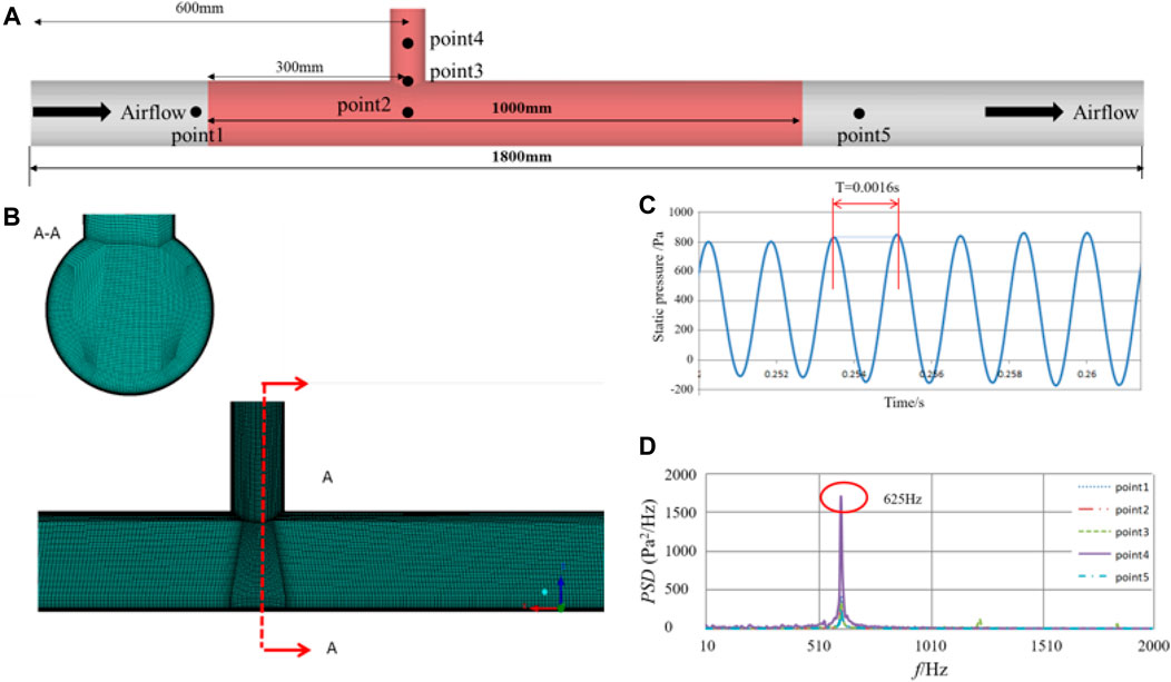
FIGURE 1. The static pressure over time and its power spectral density: (A) Monitory points of static pressure in CFD model; (B) middle plane of CFD mesh; (C) the static pressure over time of point1; (D) the power spectral density of the five points.

The surface and volume meshes of the computational domain were created using ICEM meshing tools. The size of the straight pipe and pipe valve was 4 mm. Furthermore, the height of the first boundary layer mesh was 0.05 mm to ensure that y+ ≈4.0 at an inlet velocity of 80 m/s. The growth rate and the number of layers were 1.2 and 15, respectively. The boundary layer mesh was applied to all the surfaces, while its quality was acceptable. The total number of grids totaled about 3.9 million, and the middle plane of the grid is depicted in Figure 1B.

The incoming velocity of the computational domain inlet was 80 m/s, while the pressure of the computational domain outlet was 0 Pa. The wall boundary conditions were used on the surfaces of the straight pipe and pipe valve. A compressible model and a pressure-based solver were used to carry out the aerodynamic calculations. The discretization of pressure, momentum, and energy were second-order upwind for steady calculations, but the momentum discretization changed into bounded central differencing for unsteady calculations. First, the realizable k-epsilon was run to initialize the flow field in 5,000 iterations, helping to obtain a quick and robust convergence of unsteady simulation. Then, the computation transformed into an unsteady state. LES started to run in a time-step of 0.0001 s with 25 iterations in each time-step. The duration of 0.3 s was roughly 13 times the flow-through time from inlet to outlet. The data sampling began after the flow field reached instability. Data sampling was conducted for 1,000 time-steps, while no universal criterion was available for judging the convergence. Consequently, during this investigation, the calculation was considered convergent when each variable met the convergence criteria, which was about 10⁻⁴. Furthermore, the pressure and velocity were monitored to confirm that the flow field variable did not change after multiple iterations.

Over time, the static pressures of the five measuring points in the flow field showed that it displayed a typical periodicity. Figure 1C showed the change curve of the static pressure with time for measuring point1, whose duration was 0.0016 s. The power spectral density analysis of each measuring point revealed a significant peak near 625 Hz in Figure 1D, which was significantly higher than the other frequencies. Point4 was located in the pipe valve, and exhibited the largest peak value, while point1 was upstream of the pipe valve pipe and displayed the smallest peak value. For the current straight pipe with a pipe valve, an acoustic resonance phenomenon occurred, while the resonance frequency was calculated using Eq. 8. The theoretical calculation frequency was consistent with the current unsteady flow field simulation calculation frequency, indicating the accuracy of the unsteady flow-field simulation method.

f = \frac{(2 n - 1) c}{4 (L - \frac{8 r}{3 π})} (8)

Wherein, n is the resonance order; L is the length of the pipe valve; r is the radius of the cavity.

Furthermore, to clearly reflect the changes in the flow field during a specific period, the velocity contour of three periods in the middle plane was chosen. Figure 2 shows that the area displaying large velocity fluctuations was concentrated inside and downstream of the pipe valve. The current structure belonged to an open cavity, and the diameter was smaller than the length. For the open cavity, the shear layer formed at the front end of the pipe valve, and the developed shedding vortex propagated downstream, directly hitting the rear end of the pipe valve. Due to the vortex impact, a feedback compression wave propagating upstream was generated in the trailing edge of the cavity. The feedback compression wave propagated upstream and finally reached the leading edge of the cavity. Consequently, noise disturbance was induced, the shear layer of the leading edge was excited again, and the resonance period was closed. The periodic intermittent changes in velocity were indicative of such a flow mechanism.

FIGURE 2

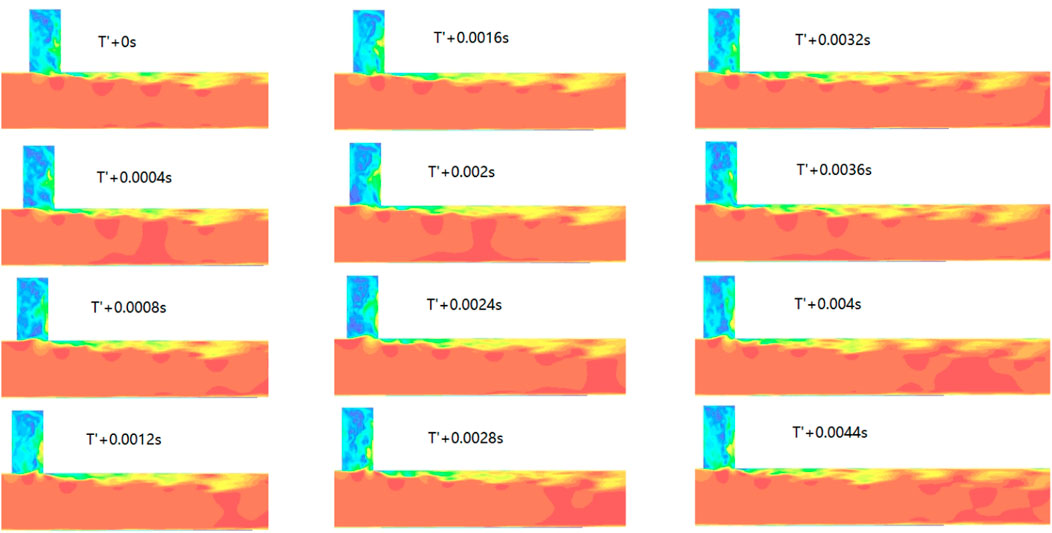
FIGURE 2. The contour of the periodic variation in the flow velocity over time

3.2 Aero-Acoustic Simulation and Experiment

Part of the fluid model was changed into an acoustic model to analyze the resonant cavity system containing a single pipe valve. The grid size of the acoustic model was 10 mm, ensuring that the point per wavelength exceeded 8at a calculation frequency of 4,000 Hz. This meets the point per wavelength requirements of about 6∼8. The velocity and density of the fluid model were converted into the sound source of the acoustic model by interpolation. Furthermore, sound propagation was performed using the Lighthill analogy in the frequency domain. The wall surface of the pipeline was reflected completely, while the end surfaces at both ends of the pipeline were defined as the modal boundary of the pipeline. When the simulated sound wave was transmitted to the end surface of the pipeline, it propagated down the pipeline without reflection, simulating the true acoustic impedance of the cross-section of the pipeline. Since both the sound source area and the sound propagation area solved the sound wave equation, the acoustic measuring points could be arranged in these locations. The noise test of the resonant pipeline systems with a single pipe valve was performed at different flow velocities, as shown in Figure 3

FIGURE 3

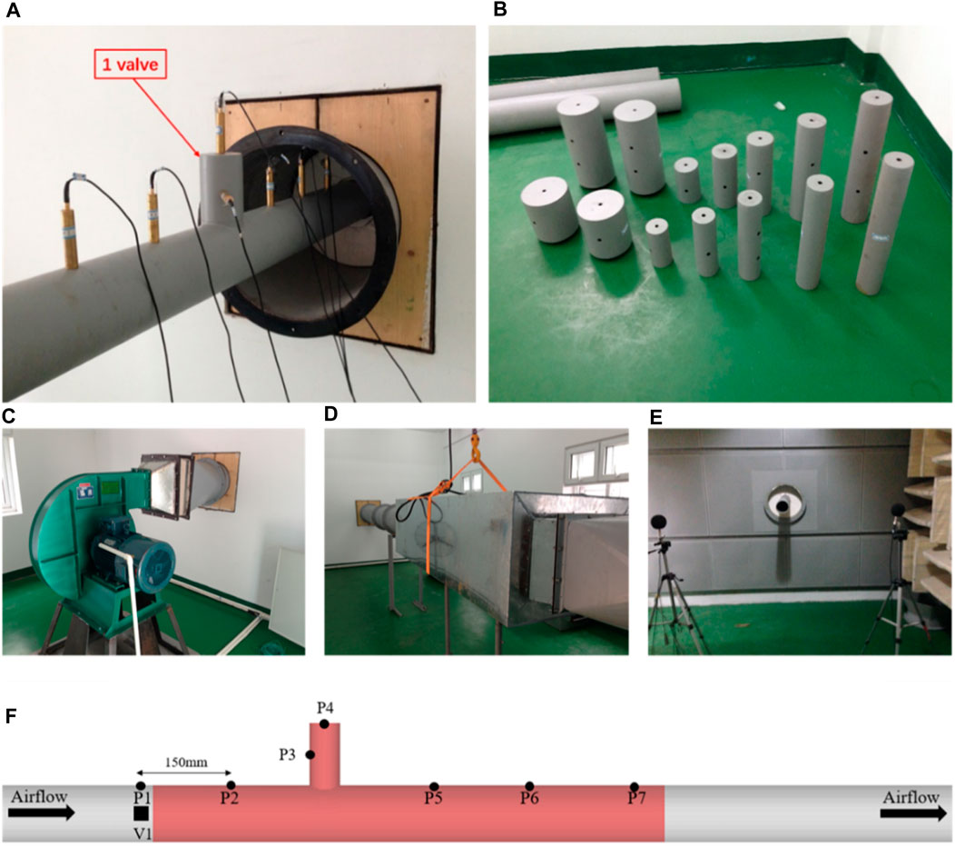
FIGURE 3. The noise test of the resonant pipeline-cavity system: (A) Single pipe valve acoustic testing system; (B) multiple types of valve resonators; (C) the airflow generation system; (D) the muffler in front of the testing system; (E) semi-anechoic room in the end; (F) Pressure fluidization and velocity monitors in CFD model.

The test facility included an airflow generation system, test piping, and the test system. The airflow system was composed of an air storage tank, flow control valve, straight pipe, front-stage reducer, rear exhaust port, and muffler room, which could produce an airflow up to 100 m/s. As shown in Figure 3B, for exploring the influence of different shapes and sizes of the valves on the acoustic results, multiple types of valve resonators with different sizes were selected in the experiment, including but not limited to an L11 model (with valve size ∅ 6 * 12 cm), L12 model (with valve size ∅ 6 * 24 cm), and L13 model (with valve size ∅ 4 * 12 cm). Finally, the L11 model was selected for research and is described in this paper.

The test pipeline system consisted of the main pipeline and the resonant cavity. Due to the high airflow velocity of the resonant cavity, the front end of the microphone was placed as close to the inner wall of the straight pipe and pipe valve as possible to reduce the impact of the airflow on the microphone and to truly reflect the airflow noise in both locations. Moreover, a small amount of porous sound-absorbing material was placed in front of the microphone, which acted as a windproof ball. For the single valve system, seven measuring points were arranged on the straight pipe and the pipe valve, and are shown in Figure 3C. P1 and P2 were arranged upstream of the straight pipe, while P5∼P7 were located downstream of the straight pipe. The distance between the two measuring points was 150 mm. P3 was located in the center of the side of the pipe valve, and P4 was arranged on top of the pipe valve.

A 1/4 inch MP401 pressure field microphone was used to collect the sound pressure at different airflow velocities, while the velocity in the straight pipe was measured using a Testo 512 differential pressure measuring instrument. An SQlab multi-channel, real-time analyzer was used to collect and assess the sound pressure. It should be noted that no interference was evident from other strong sound sources in the test environment. All the test data can be used to create a relationship between the pipe resonance cavity and the sound field, verifying the hybrid simulation method.

The simulation and test results of the upstream and downstream acoustic measuring points of the pipe valve were selected and compared, as shown in Figure 4A. For the upstream measuring point P2, the simulated value of the first-order resonance frequency and magnitude was smaller than the test value 130 dB at about 625 Hz. However, the difference in the second-order resonance frequency and magnitude exhibited an increase, while the values of the third-order resonance were even more significant. Overall, the simulation of the sound pressure level (SPL) in a frequency band below 1800 Hz corresponded well with the experiment, but the agreement at higher frequencies was poor. For the downstream measuring point P5 in Figure 4B, the first-order resonance frequency did not differ much, but the magnitude displayed substantial differences. Except for the frequency exceeding 1800 Hz, the simulated value of the SPL of other frequencies differed little from the experimental value, while the overall agreement was good.

FIGURE 4

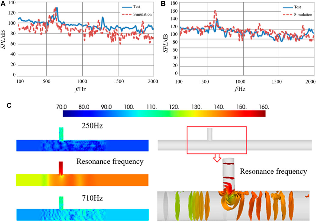
FIGURE 4. The SPL curve and contour at different frequencies/dB: (A) The SPL curve of P2; (b) the SPL curve of P5; (C) the sound pressure contour at different frequencies.

The resonant frequency and the SPL contour of the other two frequencies are shown in Figure 4C, indicating that when acoustic resonance occurred, the sound pressure in the pipe was much more substantial than that of other frequencies, and the sound pressure in the pipe valve exceeded that of the straight pipe. Furthermore, the downstream sound pressure of the pipe was higher than the upstream. The frequency characteristics and acoustic resonance intensity could be improved by changing the form and position of the pipe valve, such as the rounding of the connection.

The following section analyzes the resonance characteristics of different speeds based on the test results. Figure 5 shows that the overall sound pressure level (OSPL) of the test point inside the pipe valve at the same airflow velocity was significantly higher than that of other test points in the straight pipe.

FIGURE 5

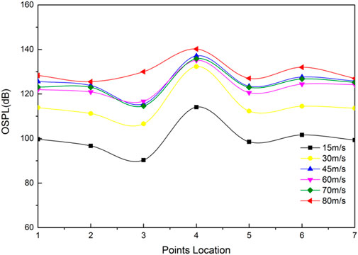
FIGURE 5. OSPL at different velocities (test results).

The OSPL increased rapidly in conjunction with an increase in the velocity from 15 m/s to 45 m/s, showing a gradual rise as the velocity increased from 60 m/s to 80 m/s. Due to the acoustic cavity resonance, OSPL depended on the resonance peak. The OSPL of the same test point at a velocity of 45 m/s was higher than at 70 m/s. The small difference between the resonance peaks of 60 m/s to 70 m/s resulted in a small OSPL difference. The Strouhal number defined by Eq. 9 was 0.83 at a velocity of 45 m/s and decreased to 0.47 at a velocity of 80 m/s, so found that the corresponding Strouhal number range was [0.47, 0.83].

S_{t} = \frac{f d}{v} (9)

Here, f is the acoustic resonance frequency, d is the diameter of the pipe valve, and v is the velocity.

4 Application 1: Single-Valve System Used for Generated Sound Source

4.1 Model Introduction

In this application, airflow through a single valve or branch duct system produced a big aerodynamic noise, which was used as a sound source in subsequent experiments. The inner diameter of the main pipe was 110 mm, and the diameters of the different branch ducts were 60 and 90 mm (with chamfering). As showed in Figure 6, the airflow was generated by an air tank, and the pressure in the main pipe was adjusted by the pressure control valve. When the airflow flowed through the valve/side branch within a certain velocity range, obvious acoustic resonance was generated in the pipe. The flow rate of the airflow in the main pipeline was controlled by the flow control valve, and finally went to the external free field through the exhaust muffler exhaust. The adjustment range of the pressure control valve was 0.3 ∼ 0.7 mpa; the adjustable valve can control the flow rate in the main pipe from 20 m/s to 80 m/s.

FIGURE 6

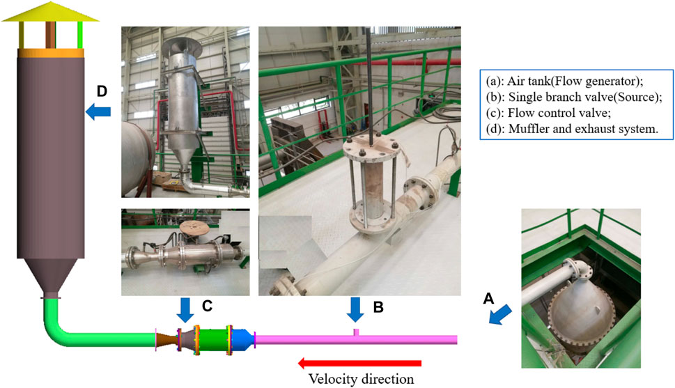
FIGURE 6. Aero-Acoustics source generation system.

4.2 Simulation and Regular Models

The straight pipeline and valve department shown in the experiment were taken as the analysis object in the CFD calculation, and all the settings of the boundary condition and turbulence model are consistent with the model setting methods in Section 3. The side branch pipe model with a diameter of 90 mm with chamfering was selected; the inlet velocity in the main pipeline was 50 m/s, and the outlet pressure in the pipeline was set to 0.4 MPa. Taking the pressure fluctuation values of the monitor within the valve during the transient CFD calculation, the corresponding curve is shown by the blue line in the figure below. The Pressure Fluctuation gradually presents periodicity after 0.32 s.

As shown in Figure 7, the time-domain curve in the above figure was processed by discrete Fourier transform (DFT) to obtain the pressure fluctuation in the frequency domain, as shown by the red line. There were several obvious characteristic peaks in the red line, corresponding to 300 Hz and its harmonic frequencies. These frequencies and peaks corresponded to the frequency (Hz) and pressure fluidizations (dB) of loadcase_5 in the monitors in branch duct column in the following Table 1.

FIGURE 7

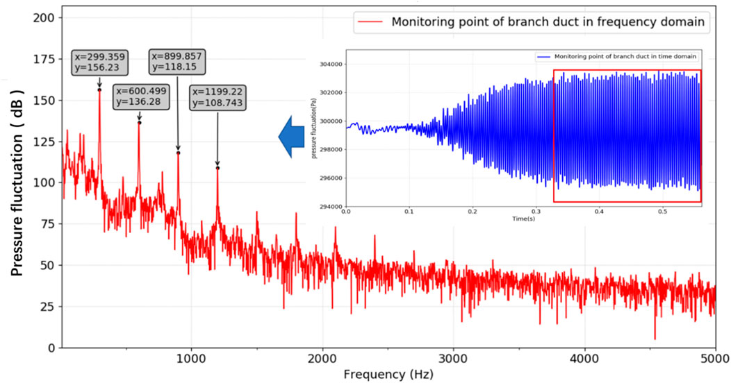
FIGURE 7. Pressure fluctuation across time (blue) and frequency (red).

TABLE 1

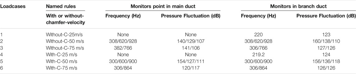
TABLE 1. The frequencies and dB value of pressure fluctuation in main duct and branch duct from CFD.

As shown in Table 1, there was no acoustic resonance in loadcase_1 and loadcase_4 and there was no obvious characteristic frequency. In loadcase_2 and loadcase_5 there occurred obvious acoustic resonance with three obvious characteristic frequencies and characteristic peaks, respectively. The resonance frequency was concentrated at 300 Hz and its harmonic frequencies and the pressure fluctuation amplitude was much higher than in other working conditions. Obviously, loadcase_5 was the working condition with the strongest SPL in the main pipe, and loadcase_2 was the working condition with the strongest SPL in the resonant cavity\branch pipe.

We imported the CFD data into the CAA program for aero-acoustic calculation, and the simulation results were compared against and verified with the experimental results. The branch duct model without a chamfer and with an inner diameter of 60 mm and height of 250 mm was selected for description. As shown in Table 2, there were 3 obvious characteristic peaks in the experimental and simulation results of acoustic resonance phenomena with different flow velocity conditions, and the results of numerical simulation were in good agreement with the experimental data. When the flow velocity was 50 m/s, the maximum SPL of acoustic resonance reached 179dB, which was much larger than the SPL of velocity at 25 m/s and 75 m/s.

TABLE 2

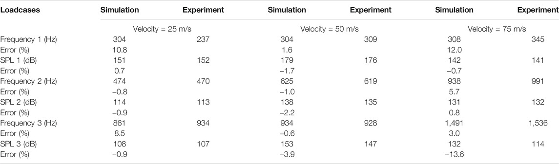
TABLE 2. Frequencies and SPL of acoustic resonance comparison between simulation and experiment when the diameter (without chamfer) and height of the branch pipe were 60 and 250 mm, respectively.

5 Application 2: The Aero-Acoustics Analysis of the Multi-Valves

5.1 Numerical Model and Sound Field Prediction

The acoustic test of the resonant pipeline-cavity system with six-pipe valves was performed at different flow velocities, as shown in Figure 8. For the multiple-valve system, the effective length and inner diameter of the straight pipe were 9,000 mm and 305 mm, respectively, while the pipe valve had an inner diameter of 64 mm and a length of 500 mm. The pipe valve spacing was about 1,000 mm. For the multiple-valve system, twelve measuring points were arranged on the six-pipe valves, and are shown in Figure 8A. Two measuring points were arranged on each pipe valve at space intervals of 80 mm. A flow velocity measuring point was established in the pipeline system, while there was 300 mm in front of the resonant cavity.

FIGURE 8

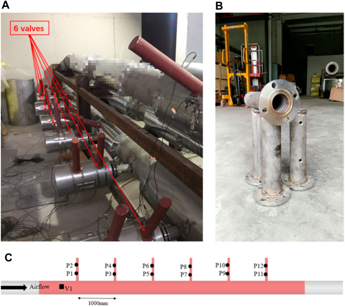
FIGURE 8. The noise test of the resonant pipeline-cavity system: (A) Six pipe valves; (B) microphone location in the test; (C) sound pressure monitors in acoustic model.

The numerical model of the straight pipe containing six-pipe valves was created, which was consistent with the test. The length of the computational domain was 9,000 mm, about 30 D (D is the diameter of the pipe valve). There was a distance of 2000 mm from upstream of the pipe valve and a 2000 mm downstream distance. All the acoustic measuring point positions of the six-pipe valves were the same as in the test. The surface and volume meshes of the computational domain were created via ICEM. The average sizes of the straight pipe and pipe valves were 8 mm. Furthermore, the height of the first boundary layer mesh was 0.03 mm to ensure y+≈2.0 when the inlet velocity was 65 m/s. The growth rate and the number of layers were 1.2 and 15, respectively. The boundary layer mesh was applied to all the surfaces, and the mesh quality was acceptable. The total number of grids was about 26.6 million, and the middle plane of the grid is depicted in Figure 9. The velocity entering the inlet of the computational domain was 65 m/s, while it displayed the strongest acoustic resonance. The boundary conditions and calculation process were consistent with that of the single pipe valve, and will not be repeated here.

FIGURE 9

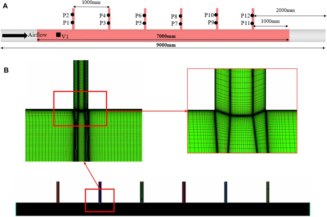
FIGURE 9. Computational domain and the middle plane of the grid: (A) Computational domain; (B) middle plane of the grid.

Part of the fluid model was changed into an acoustic model to analyze the resonance cavity system with six-pipe valves. The grid size of the acoustic model was 20 mm, ensuring that the point per wavelength exceeded 8 if the calculation frequency was 2000 Hz. The sound field was predicted using the transient flow and Lighthill analogy, while the boundary conditions and calculation process were also consistent with that of the single-pipe valve system, which will not be repeated here.

P3 and P5 were chosen to compare the differences between the sound pressure levels of the simulation and test results, as shown in Figure 10. The first-order resonance frequency of 480 Hz and the second-order resonance frequency of 820 Hz were found at the SPL spectrums of the simulation and test. However, their magnitudes were distinctly different. As for P3, the simulated values of the first-order resonance peak and the second-order resonance peak were about 10 and 9 dB different from the test value. Smaller differences were evident for P5, where only a 3 dB difference was apparent. Overall, the simulation of the SPL in the frequency band below 1,250 Hz corresponded well with the test, matching the cut-off frequency.

FIGURE 10

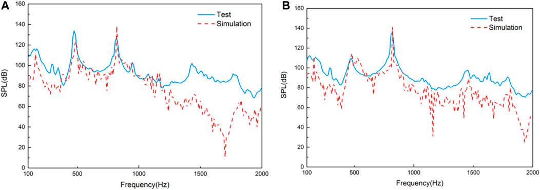
FIGURE 10. The SPL spectrum comparative curves of different points: (A) P3 SPL curves; (B) P5 SPL curves.

The SPL contours of the first-order and second-order resonance frequencies are shown in Figure 11, indicating that when acoustic resonance occurred, the sound pressure in the pipe valve exceeded that of the straight pipe. The SPL of the second-order resonance frequency was higher than that of the first-order resonance frequency, for which the SPL of the third pipe valve was the lowest, but changed to the sixth pipe valve for the second-order resonance frequency.

FIGURE 11

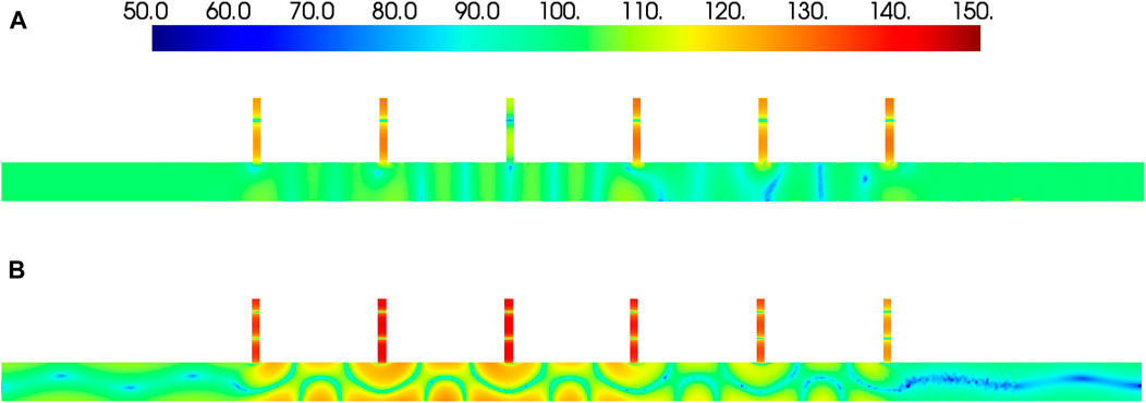
FIGURE 11. Sound pressure contour at different frequencies/dB: (A) The SPL contours of 490Hz; (B) the SPL contours of 820 Hz.

5.2 The Sound Field Prediction via SNGR and Steady Flow

The stochastic noise generation and radiation (SNGR) method re-synthesized the flow field data containing the time term based on the time-averaged velocity and turbulent kinetic energy obtained from the Reynolds Averaged Navier-Stokes calculation results by adding random perturbations. The turbulent pulsation velocity in Eq. 10 and Eq. 11 was synthesized using a stochastic model approach, which could be derived from the N Fourier modes. SNGR produced sound sources equivalent to volume Lighthill analogy sources in the frequency domain, as shown in Eq. 12. SNGR is based on stochastic isotropic turbulence theory, which is suitable for noise generated by small-scale eddies. It was challenging for SNGR to predict noise generated by middle- and large-scale eddies, however, this is exactly what traditional CFD and the Lighthill analogy can do. Therefore, a hybrid simulation method combining LES, the Lighthill analogy, and SNGR was used to predict the aerodynamic noise generated by the resonant cavities of pipeline valves.

u_{i}^{t} (x_{j}, t) = 2 \cdot \sum_{n}^{N} {\tilde{u}}^{n} \cos (K^{n} k_{j}^{n} x_{j} + φ^{n} + ω^{n} \cdot t) \cdot σ_{j}^{n} (10)

{\tilde{u}}^{n} = \sqrt{E (K^{n}) Δ K^{n}} (11)

\int_{Ω} N_{a} \frac{\partial^{2} T_{i j}}{\partial x_{i} \partial x_{j}} d Ω = \int_{V} \frac{J}{ρ_{0} ω} ρ \frac{\partial N}{\partial x_{i}} \frac{\partial}{\partial x_{j}} (u_{i}^{t} \otimes u_{j}^{t}) (f) d V (12)

Here, $E (k^{n})$ is the turbulent energy density spectrum and $S_{t} = \frac{f d}{v}$ is the wavenumber step; $S_{t} = \frac{f d}{v}$ is the angular turbulent frequency associated with the $n^{t h}$ velocity mode; $S_{t} = \frac{f d}{v}$ is the random phase associated with the $n^{t h}$ velocity mode; $k^{n}$ is the turbulent wavenumber associated with the $n^{t h}$ velocity mode; $S_{t} = \frac{f d}{v}$ is the random orientation of turbulent wave vector associated with the $n^{t h}$ velocity mode; $S_{t} = \frac{f d}{v}$ corresponds to the direction of the $n^{t h}$ velocity mode and is restricted in a plane perpendicular to $k_{j}^{n}$ to ensure mass conservation; $\otimes$ denotes the convolution product; and f is the maximum frequency deduced from the Kolmogorov wavenumber.

A requirement for aero-acoustic simulations based on unsteady CFD data demands that the CFD mesh supports the maximum frequency targeted by the user, which is called the mesh cut-off frequency and depends on the turbulent quantities and the cell size presented in the CFD mesh. The cut-off frequency was defined according to Eq. 13 and Eq. 14. Due to the significant turbulence dissipation rate and large grid size, the cut-off frequency in the main stream of the pipe was about 1800 Hz, which was consistent with the distortion frequency shown in Figure 12. One challenge pertained to what could be done in cases where higher frequency noises might be important.

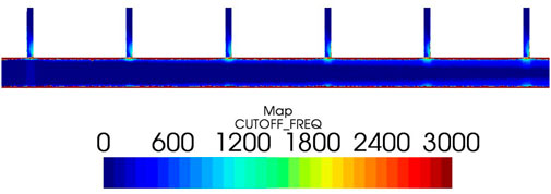
F c u t - o f f = A \times k^{α} \times ε^{β} \times Δ x^{γ} (13)

FIGURE 12

FIGURE 12. Cut-off frequency map of multiple valves.

By following the Buckingham π theorem (Buckingham, 1914),

F c u t - o f f = A \times k^{α} \times ε^{β} \times Δ x^{γ} = k^{α} \times ε^{\frac{1}{3} (1 - 2 α)} \times Δ x^{- \frac{2}{3} (1 + α)} \approx ε^{\frac{1}{3}} \times Δ x^{- \frac{2}{3}} (α = 0) (14)

Here, k is the turbulent kinetic energy, Ɛ is the turbulent dissipation rate, and Δx is the element size.

SNGR could be used as a method for rapidly predicting the turbulent noise of middle and high frequencies. It generated several realizations of the turbulent velocity field, respecting experimental and theoretical characteristics of the turbulence. Only the velocity, turbulent kinetic energy, and turbulent dissipation rate of the steady-state calculation were exported into the Aero-Acoustics computation procedure as sound sources. The sound propagation was performed using the Lighthill analogy and the same boundary conditions to obtain the sound pressures of both the near-field and far-field. Furthermore, the SNGR and steady flow method was adopted to obtain the sound pressure at a higher frequency, and their comparison results are shown in Figure 13.

FIGURE 13

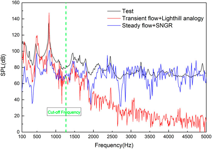
FIGURE 13. The SPL spectrum of P5 for different methods.

The results of the transient flow and the Lighthill analogy corresponded well with the test results below the 1,250 Hz frequency, while their differences gradually increased as the frequency became higher. The blue curve shows that the result of steady flow and SNGR from 1,250 Hz to 5,000 Hz corresponded well with the test. Considering the calculation time and grid complexity of the two calculation methods, it was recommended again that the method involving transient flow and the Lighthill analogy be used for low frequencies while applying the technique involving steady flow and SNGR to middle and high frequencies for similar problems.

6 Conclusion

The resonance cavity system with either a single pipe valve or six-pipe valves was investigated via numerical simulation and testing. The traditional method involving unsteady flow and the Lighthill analogy was used to understand the fluid and acoustic characteristics of the resonant cavity system. The acoustic resonance phenomenon occurred within a specific velocity range with 45 m/s and 80 m/s, and the strongest acoustic resonance appeared at a velocity of 80 m/s; the corresponding Strouhal number range was [0.47, 0.83]. The energy of the acoustic resonance was primarily concentrated in the pipe valve.

The traditional method allows for the acquisition of an SPL below the cut-off frequency that displays excellent consistency between the simulation and the test. However, more substantial differences are evident as the frequency increases. A new method involving steady flow and SNGR is proposed to solve the differences encountered at middle and high frequencies. The consistency of the entire frequency band shows that combining the traditional method with this new technique is the ideal choice when confronted with limited time and computer resources. Therefore, it is recommended that the traditional method involving transient flow and the Lighthill analogy be used for low frequencies while applying this new technique involving steady flow and SNGR to middle and high frequencies for similar problems.

Data Availability Statement

The original contributions presented in the study are included in the article/supplementary material, further inquiries can be directed to the corresponding authors.

Author Contributions

CB: Mainly creator of the manuscripts; Derivation of the theoretical formula; Experimental data collector; Simulation soft-ware operator. TC: Idea of the innovative in the paper; Development and design of the relevant methodology; Providers of the funding project and experimental environments. WY: Experimental equipment provider; Paper data processing; Article proofs.

Funding

This work was supported by the National Natural Science Foundation of China (Grant No. 11874290) and the Major National R&D Project (Grant No.2019ZX06004001).

Conflict of Interest

The authors declare that the research was conducted in the absence of any commercial or financial relationships that could be construed as a potential conflict of interest.

The handling editor declared a shared affiliation with several of the authors CB and TC at the time of review.

Publisher’s Note

All claims expressed in this article are solely those of the authors and do not necessarily represent those of their affiliated organizations, or those of the publisher, the editors and the reviewers. Any product that may be evaluated in this article, or claim that may be made by its manufacturer, is not guaranteed or endorsed by the publisher.

References

Alber, T. H., Gibbs, B. M., and Fischer, H. M. (2011). Characterisation of Valves as Sound Sources: Fluid-Borne Sound. Appl. Acoust. 72 (7), 428–436. doi:10.1016/j.apacoust.2011.01.007

CrossRef Full Text | Google Scholar

Alber, T. H., Gibbs, B. M., and Fischer, H. M. (2009). Characterisation of Valves as Sound Sources: Structure-Borne Sound. Appl. Acoust. 70 (5), 661–673. doi:10.1016/j.apacoust.2008.08.002

CrossRef Full Text | Google Scholar

Alice, S. C., Marlene, S., Guillaume, L., Stephane, M., and Martin, B. (2014). “Experimental and Numerical Investigation on Noise Induced by a Butterfly Valve,” in 20th AIAA/CEAS Aeroacoustics Conference, Atlanta, GA, 16-20 June 2014 (AIAA 2014-3292). doi:10.2514/6.2014-3292

CrossRef Full Text | Google Scholar

Bailly, C., and Juve, D. (2012). “A Stochastic Approach to Compute Subsonic Noise Using Linearized Euler’s Equations,” in 5th AIAA/CEAS Aeroacoustics Conference and Exhibit, Bellevue,WA,U.S.A., 10 May 1999 - 12 May 1999 (AIAA). doi:10.2514/6.1999-1872

CrossRef Full Text | Google Scholar

Bailly, C., Lafon, P., and Candel, S. (2012). “Computation of Noise Generation and Propagation for Free and Confined Turbulent Flows,” in 2th AIAA/CEAS Aeroacoustics Conference, State College,PA,U.S.A., 06 May 1996 - 08 May 1996 (AIAA 1996-1732). doi:10.2514/6.1996-1732

CrossRef Full Text | Google Scholar

Bechara, W., Bailly, C., Lafon, P., and Candel, S. M. (1994). Stochastic Approach to Noise Modeling for Free Turbulent Flows. AIAA J. 32 (3), 455–463. doi:10.2514/3.12008

CrossRef Full Text | Google Scholar

Buckingham, E. (1914). On Physically Similar Systems; Illustrations of the Use of Dimensional Equations. Phys. Rev. 4 (4), 345–376. doi:10.1103/physrev.4.345

CrossRef Full Text | Google Scholar

Charlebois-Menard, M., Sanjose, M., Aurelien, M., Chauvin, A., Pasco, Y., Moreau, S., and Brouillette, M. (2015). “Experimental and Numerical Study of the Noise Generation in an Outflow Butterfly Valve,” in 21th AIAA/CEAS Aeroacoustics Conference, Dallas, TX, USA, June 22-26, 2015 (AIAA 2015-3123). doi:10.2514/6.2015-3123

CrossRef Full Text | Google Scholar

Du, J., and Ouyang, H. (2010). Experimental Study of Whistle Noise Generated by Insert Edge and Oil Separator Model of Refrigeration Cycle. Appl. Acoust. 71 (7), 597–606. doi:10.1016/j.apacoust.2010.01.011

CrossRef Full Text | Google Scholar

Durgin, W. W., and Graf, H. R. (1992). “Flow Excited Acoustic Resonance in a Deep Cavity,” in Symposium on Flow-Induced Vibration and Noise. AMD-Vol. 151/PVP-Vol. 247, Volume 7 (ASME).

Google Scholar

Germano, M., Piomelli, U., and Moin, P. (1991). A Dynamic Subgrid-Scale Eddy Viscosity Model. Phys. Fluids 3, 1760–1765. doi:10.1063/1.857955

CrossRef Full Text | Google Scholar

Lesieur, M., and Metais, O. (1996). New Trends in Large-Eddy Simulations of Turbulence. Annu. Rev. Fluid Mech. 28 (1), 45–82. doi:10.1146/annurev.fl.28.010196.000401

CrossRef Full Text | Google Scholar

Lighthill, M. J. (1952). On Sound Generated Aerodynamically I. General Theory. Proc. R. Soc. Lond. A. 211 (1107), 564–587. doi:10.1098/rspa.1952.0060

CrossRef Full Text | Google Scholar

Lighthill, M. J. (1954). On Sound Generated Aerodynamically II. Turbulence as a Source of Sound. Proc. R. Soc. Lond. A. 222 (1148), 1–32. doi:10.1098/rspa.1954.0049

CrossRef Full Text | Google Scholar

Lilly, D. K. (1962). On the Numerical Simulation of Buoyant Convection. Tellus 14, 148–172. doi:10.3402/tellusa.v14i2.9537

CrossRef Full Text | Google Scholar

Ma, F., Wang, C., Liu, C., and Wu, J. H. (2021). Structural Designs, Principles, and Applications of Thin-Walled Membrane and Plate-type Acoustic/elastic Metamaterials. J. Appl. Phys. 129, 231103. doi:10.1063/5.0042132

CrossRef Full Text | Google Scholar

Ma, T., Chen, Y., Chen, H., Zheng, Y., Huang, G., Wang, J., et al. (2021). Tuning Characteristics of a Metamaterial Beam with Lateral-Electric-Field Piezoelectric Shuntings. J. Sound Vibration 491, 115738. doi:10.1016/j.jsv.2020.115738

CrossRef Full Text | Google Scholar

Marsan, A., Sanjose, M., Yann, P., Stephane, M., and Martin, B. (2016). “Unsteady wall Pressure Measurements in an Outflow Butterfly Valve Using Remote Microphone Probes,” in 22th AIAA/CEAS Aeroacoustics Conference, Lyon, France, 30 May - 1 June, 2016 (AIAA 2016-2888). doi:10.2514/6.2016-2888

CrossRef Full Text | Google Scholar

Oldham, D. J., and Waddington, D. C. (2001). The Prediction of Airflow-Generated Noise in Ducts from Considerations of Similarity. J. Sound Vibration 248 (4), 780–787. doi:10.1006/jsvi.2001.3721

CrossRef Full Text | Google Scholar

Paolo, D. F., Charles, H., Piergiorgio, F., and Katsutomo, I. (2015). “Side Mirror Noise with Adaptive Spectral Reconstruction,”. SAE Technical Papers (SAE 2015-01-2329).

Google Scholar

Paolo, D. F., Piergiorgio, F., Thomas, D., and Charles, H. (2013). “Assessment of SNGR Method for Robust and Efficient Simulations of Flow Generated Noise,” in 19th AIAA/CEAS Aeroacoustics Conference, Berlin, Germany, May 27-29, 2013 (AIAA 2013-2264). doi:10.2514/6.2013-2264

CrossRef Full Text | Google Scholar

Pelat, A., Gautier, F., Conlon, S. C., and Semperlotti, F. (2020). The Acoustic Black Hole: A Review of Theory and Applications. J. Sound Vibration 476, 115316. doi:10.1016/j.jsv.2020.115316

CrossRef Full Text | Google Scholar

Ryu, J., Cheong, C., Kim, S., and Lee, S. (2005). Computation of Internal Aerodynamic Noise from a Quick-Opening Throttle Valve Using Frequency-Domain Acoustic Analogy. Appl. Acoust. 66 (11), 1278–1308. doi:10.1016/j.apacoust.2005.04.002

CrossRef Full Text | Google Scholar

Shih, T.-H., Liou, W. W., Shabbir, A., Yang, Z., and Zhu, J. (1995). A New K-ϵ Eddy Viscosity Model for High reynolds Number Turbulent Flows. Comput. Fluids 24 (3), 227–238. doi:10.1016/0045-7930(94)00032-t

CrossRef Full Text | Google Scholar

Shiro, T., Masaya, O., Keita, O., Takashi, I., and Kazuhiro, Y. (2008). Experiment Study of Acoustic and Flow-Induced Vibrations in BWR Main Steam Lines and Steam Dryers. ASME 2008 Press. Vessels Piping Conf. 7, 27–31.

Google Scholar

Uchiyama, Yuta., and Morita, Ryo. (2015). “Experimental Investigation for Acoustic Resonance in Tandem Branches under Each Dry and Wet Steam Flow,” in Pressure Vessels and Piping Conference, November 19, 2015 (Boston, MA: PVP2015-45456, ASME).

CrossRef Full Text | Google Scholar

Zhu, R., Liu, X. N., Hu, G. K., Sun, C. T., and Huang, G. L. (2014). A Chiral Elastic Metamaterial Beam for Broadband Vibration Suppression. J. Sound Vibration 333, 2759–2773. doi:10.1016/j.jsv.2014.01.009

CrossRef Full Text | Google Scholar

Ziada, S., and Shine, S. (1999). Strouhal Numbers of Flow-Excited Acoustic Resonance of Closed Side Branches. J. Fluids Structures 13 (1), 127–142. doi:10.1006/jfls.1998.0189

CrossRef Full Text | Google Scholar

Keywords: resonance system, pipe valve, steady and unsteady flow, lighthill analogy, stochastic noise generation and radiation

Citation: Bai C, Chen T and Yu W (2021) Numerical and Experimental Research on Single-Valve and Multi-Valve Resonant Systems. Front. Mater. 8:756158. doi: 10.3389/fmats.2021.756158

Received: 10 August 2021; Accepted: 06 September 2021;
Published: 27 September 2021.

Edited by:

Fuyin Ma, Xi’an Jiaotong University, China

Reviewed by:

Jian-Cheng Cai, Zhejiang Normal University, China
Kai Zhang, Ocean University of China, China

Copyright © 2021 Bai, Chen and Yu. This is an open-access article distributed under the terms of the Creative Commons Attribution License (CC BY). The use, distribution or reproduction in other forums is permitted, provided the original author(s) and the copyright owner(s) are credited and that the original publication in this journal is cited, in accordance with accepted academic practice. No use, distribution or reproduction is permitted which does not comply with these terms.

*Correspondence: Tianning Chen, tnchen@mail.xjtu.edu.cn; Wuzhou Yu, ywzh@tongji.edu.cn

ORIGINAL RESEARCH article

Numerical and Experimental Research on Single-Valve and Multi-Valve Resonant Systems

1 Introduction

2.The Methodology of the Resonant Pipeline-Cavity System

2.1 Unsteady CFD Simulation

2.2 Lighthill Analogy for Aero-Acoustic Simulation

3. Aero-Acoustic Analysis of the Single Pipe Valve

3.1 CFD Simulation Analysis

3.2 Aero-Acoustic Simulation and Experiment

4 Application 1: Single-Valve System Used for Generated Sound Source

4.1 Model Introduction

4.2 Simulation and Regular Models

5 Application 2: The Aero-Acoustics Analysis of the Multi-Valves

5.1 Numerical Model and Sound Field Prediction

5.2 The Sound Field Prediction via SNGR and Steady Flow

6 Conclusion

Data Availability Statement

Author Contributions

Funding

Conflict of Interest

Publisher’s Note

References

This article is part of the Research Topic

People also looked at