
A Modeling Study of Rainbands Upstream from Western Japan during the Approach of Typhoon Tokage (2004)

1
Department of Earth Sciences, National Taiwan Normal University, Taipei 11677, Taiwan
2
Institute for Space-Earth Environmental Research, Nagoya University, Nagoya 464-8601, Japan
3
Central Weather Bureau, Taipei 100006, Taiwan
4
Department of Environmental Atmospheric Sciences, Pukyong National University, Busan 48513, Korea
*
Author to whom correspondence should be addressed.
Atmosphere 2021, 12(10), 1242; https://doi.org/10.3390/atmos12101242
Submission received: 20 August 2021
/
Revised: 18 September 2021
/
Accepted: 20 September 2021
/
Published: 23 September 2021
(This article belongs to the Section Meteorology)
Abstract
:During 19–20 October 2004, a series of spectacular arc-shaped rainbands developed south or southeast of southwestern Japan when Typhoon Tokage (TY0423) approached the region from the southwest. As the typhoon moved closer and the upstream Froude number (Fr) continued to increase, these rainbands first remained quasi-stationary but eventually retreated backward. Using the Nagoya University Cloud-Resolving Storm Simulator (CReSS) at 1-km grid size, these rainbands were successfully simulated, and their behavior during the transition period from a relatively low-Fr to a high-Fr regime was investigated and compared with idealized two-dimensional (2D) model results from theoretical studies. In the present case, the rainbands were found to develop along a low-level frontal convergence zone between the southerly flow associated with the typhoon and the northerly flow from the Sea of Japan. The northeasterly winds accelerated through gaps between topography and fed the offshore flow at the backside of the rainbands, producing a strong resistance that allowed the rainbands to remain stationary under significantly higher Fr values (at least 1.2) than predicted by 2D simulations (of about 0.3–0.5) for the retreat to occur in conditionally unstable flow with a convective available potential energy of about 1300 J kg−1. Typically ≤ 500 m in depth with a potential temperature (θ) deficit of 2–4 K across the rainband, the cooler offshore flow was also found to be enhanced by evaporative cooling as in some other events. The cooling effect helped the rainbands to hold their position until Fr of the upstream flow became too large, and the rainband with stronger cooling behind was able to withstand a higher Fr before retreat. Once the retreat started, the offshore layer became thinner and the θ deficit also reduced, and the rainbands were washed back by the strengthening upcoming flow.
1. Introduction
At mesoscale, there exist many mechanisms that can organize deep convection into linear or arc shape, including frontal uplift, blocking by topography, land–sea (and/or mountain–valley) breezes, interaction of vertical wind shear with updraft/downdraft, outflow boundary/density current, gravity waves, and conditional symmetric instability (e.g., [1,2,3,4,5,6,7,8,9,10]). Among them, the influence of mesoscale topography on prevailing flow has been the interest of research for several decades and is a topic especially important to islands with high terrain, such as Japan and Taiwan. When influenced by topography, the general behavior of the flow is controlled by the Froude number Fr = U/Nh, where U is the wind speed normal to the long axis of the topography, N the buoyancy oscillation frequency (N2 = (g/θ)(dθ/dz), where θ is potential temperature and g is the gravitation acceleration), and h the terrain height (e.g., [11,12,13]). In general, the flow carries enough momentum and tends to climb over the terrain and produce rain (after saturation) at the windward slopes if Fr > 1 (e.g., [14,15,16,17]). On the other hand, the blocking effect is significant and the flow tends to go around the obstacle if Fr < 1 (e.g., [18,19,20,21,22,23]).
Linked to Fr, several flow regimes have been proposed by theoretical studies using two-dimensional (2D) idealized simulations. Chu and Lin [24] examined the behavior of a conditionally unstable flow over a bell-shaped mesoscale mountain, and identified three flow regimes based on the location and propagation of the convection. Later, Chen and Lin [25] (hereafter CL05) modified the three flow regimes of [24], specified one additional (the fourth) regime, and proposed a 2D flow regime diagram (their Figure 12) [25] based on the unsaturated moist Froude number (Fw = U/Nwh, where Nw is the moist buoyancy oscillation frequency) and the convective available potential energy (CAPE). These four regimes of CL05 (their Figures 5 and 16) [25] are summarized below. The flow in regime I exhibits an upstream-propagating convective system and a transient convective system existing in the vicinity of the mountain at an earlier time. Regime II has a long-lasting orographic convective system over the mountain peak, upslope or downslope. In regime III, the flow contains a long-lasting orographic convective or mixed convective and stratiform precipitation system over the mountain peak, and a downstream-propagating convective system. The flow in regime IV has a long-lasting orographic stratiform precipitation system over the mountain and possibly a downstream-propagating cloud system. With a CAPE of 2000 J kg−1, regimes I through IV occur roughly when the value of Fw is < 0.2, 0.2–0.5, 0.5–0.8, and >0.8, respectively. Also, a higher (lower) CAPE shifts to favor the regime with a lower- (higher-) number at the same Fw, as suggested by Figure 12 [25] of CL05. Note that , where θv is the virtual potential temperature [26], and Fw is unsaturated to avoid negative values of Nw2 in conditionally unstable environments in CL05. Thus, Fw does not deviate much from Fr, as the former takes into account only the effect of moisture on density, not the effect of latent heating/cooling during phase changes.
Past observational and three-dimensional (3D) modeling studies have shown that stationary rainbands often develop ahead of the crest or on the windward slopes of mesoscale topography in a low-Fr (or Fw) regime. For instance, for Hawaii Island, whose peak is relatively high (~4 km) with a rather circular shape, Fr associated with the prevailing northeasterly trade winds tends to be low (≤0.3–0.5, [27]), and a reversal flow develops with upstream convection due to terrain blocking (e.g., [3,28,29,30,31]). Similarly, for Taiwan, which has elongated mountains peaking near 3 km, terrain blocking at low-Fr values can also lead to rainband formation and intensification upstream from the terrain (e.g., [32,33,34,35,36]). Note that in these above cases, rainbands typically occur over the windward slope or near shore and seldom develop more than 100 km upstream from the corresponding mountain peaks.
For the island chain of Japan, the averaged terrain height is lower (typically on the order of 1 km) and the blocking effect tends to be weaker. Thus, Fr can often approach or even exceed unity (high-Fr regime) with downstream propagating convection (e.g., [37,38,39]). While line-shaped convection is often found over the mountain slopes (and close to the ridge line, e.g., [40,41,42]), a few studies have reported that stationary rainbands took place under an Fr value larger than those predicted in the idealized 2D simulations of [24] and CL05, including [16,41]. The differences, however, are mostly in the range of 0.1–0.25 and reasonably small.
On 19 October 2004, a series of stationary rainbands developed south or southeast (upstream) from the terrain of southwestern Japan when Typhoon Tokage (T0423) approached from the southwest. As will be shown later, these rainbands collapsed and retreated backward, eventually back to over land, when Tokage moved closer and its low-level circulation caused the Fr to increase. In contrast to previous studies in which Fr is more or less unchanged, this case provides a unique opportunity to examine the behavior of rainbands upstream from terrain during the transition from a low-Fr to a high-Fr regime. Hence, in this study, through numerical simulation at high resolution (1 km grid spacing) and analysis of observational data, the behaviors of these rainbands are examined and compared with the results from 2D idealized studies of [24] and CL05.
The organization of this paper is as follows. The observational analysis and case overview associated with T0423 are presented in Section 2. The numerical model and experimental settings are described in Section 3. Results of model simulation are validated and presented in Section 4. Section 5 further discusses the various aspects of the rainbands and compares their behaviors with the 2D results of CL05. Finally, concluding remarks are given in Section 6.
2. Observations and Case Overview
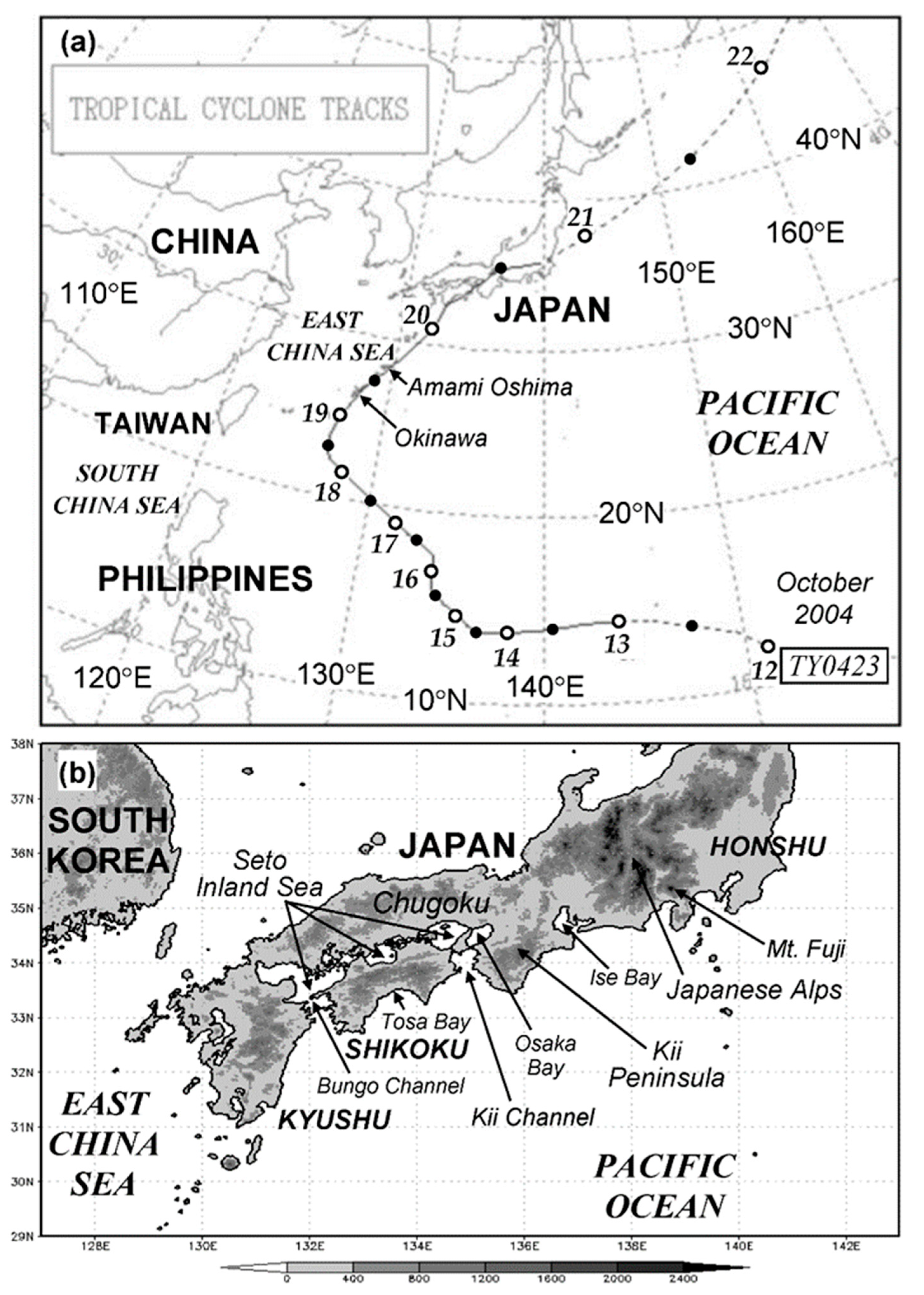
In this section, the synoptic conditions under which the arc-shaped rainbands developed and the evolution of the rainbands themselves are reviewed and discussed. First, the Japan Meteorological Agency’s (JMA’s) best-track data of Typhoon Tokage (TY0423) in October 2004 are shown in Figure 1a, while the region and topography of the focused area in this study, including western/central Japan and the adjacent area, are depicted in Figure 1b. Typhoon Tokage formed at 0000 UTC 12 October 2004 near 12° N, 151° E, reached tropical cyclone (TC) strength (≥32.7 m s−1) on 13 October, and moved at the northwest toward Taiwan and the East China Sea until 18 October (Figure 1a). Afterwards, it gradually recurved to turn northward and northeastward on 19 October and accelerated to approach southwestern Japan at a speed of over 40 km h−1. The TC center made landfall at southern Shikoku early 20 October (in UTC) and penetrated the western and central Honshu later on the same day (cf. Figure 1b), before it continued to move toward the northeast at an increasing pace, then weakened (Figure 1a). At 1200 UTC 19 October, the center of Tokage was near 27.4° N, 128.7° E, and its outer circulation produced southerly flow to blow toward Kyushu, Shikoku, and southern Honshu of Japan (cf. Figure 1b). Subsequently, several arc-shaped rainbands formed at the windward side (south or southeast) of the terrain and were maintained for several hours (to be shown shortly). These rainbands are the subject of our study.
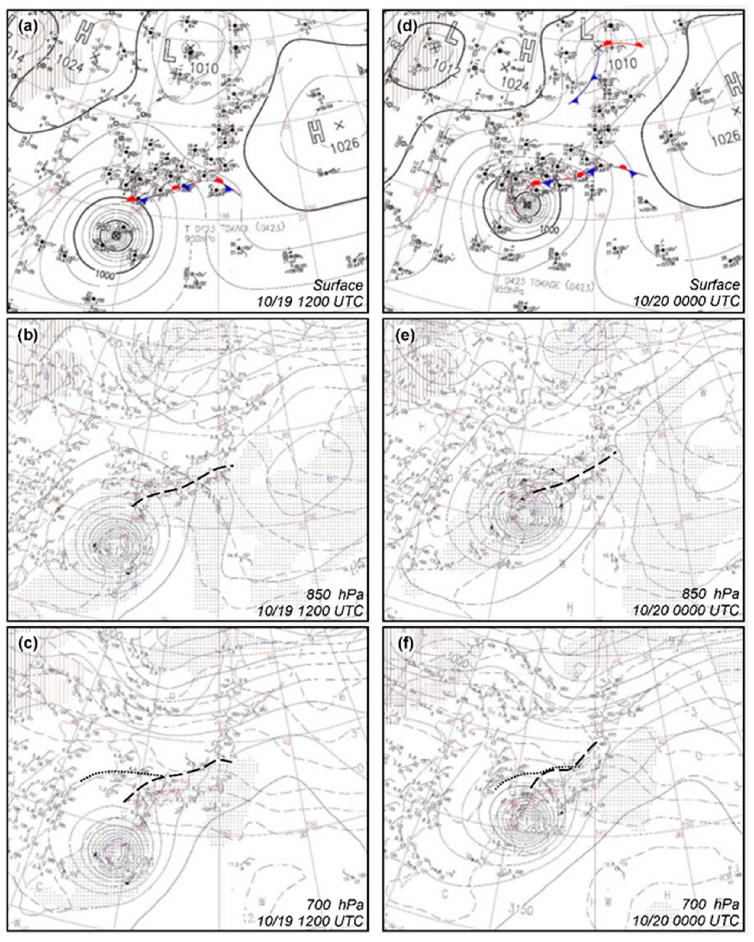
The JMA surface weather map at 1200 UTC 19 October 2004 shows that TY Tokage was southwest of Japan, as mentioned, with a central mean sea-level pressure (MSLP) of 950 hPa (Figure 2a). At this time, the subtropical Pacific High (STPH) controlled the region east and southeast of Japan, while a mid-latitude low (near 49° N, 135° E) was traveling east toward Sakhalin Island, followed by another high near 120° E. The western/central Japan was thus situated at the southern part of a saddle field, with northeasterly flow over much of the region. This northeasterly flow encountered the southerly flow east of the TC near the shorelines of Kyushu, Shikoku, and southern Honshu, where a synoptic-scale stationary front formed with an ENE–WSW orientation (Figure 1b and Figure 2a). A similar flow configuration surrounding Japan existed at 850 hPa, where the wind-shift line appeared about 150 km north of the surface front (Figure 2b). In particular, note that the winds on either side of the wind-shift line were very strong, reaching 30–40 kts ahead and 30 kts behind as well. Further up at 700 hPa, the position of the wind-shift line was another 200 km to the north and near the northern shorelines of western Japan; and southerly flows were found over much of western–central Japan at 1200 UTC 19 October (Figure 2c). When Typhoon Tokage moved closer (and the southerly flow associated with the TC got stronger) 12 h later, the synoptic flow patterns remained but the front/low-level wind-shift line was pushed back by a distance roughly 50–150 km (Figure 2d–f). Note that the northeasterly flow behind the wind-shift line further intensified during this period and could reach a speed as high as 70 kts at 850 hPa at 0000 UTC 20 October (Figure 2e). At 700 hPa, wind speeds near South Korea also picked up significantly, from 5–15 kts to 25-45 kts (Figure 2f), clearly linked to the approach of TY Tokage to the region. At 500 hPa (charts not shown), a wind-shift line between the southerly flow (associated with TC and STPH) and the mid-latitude westerlies also existed during this period, but was further west compared to the 700 hPa one (cf. Figure 2c,f).
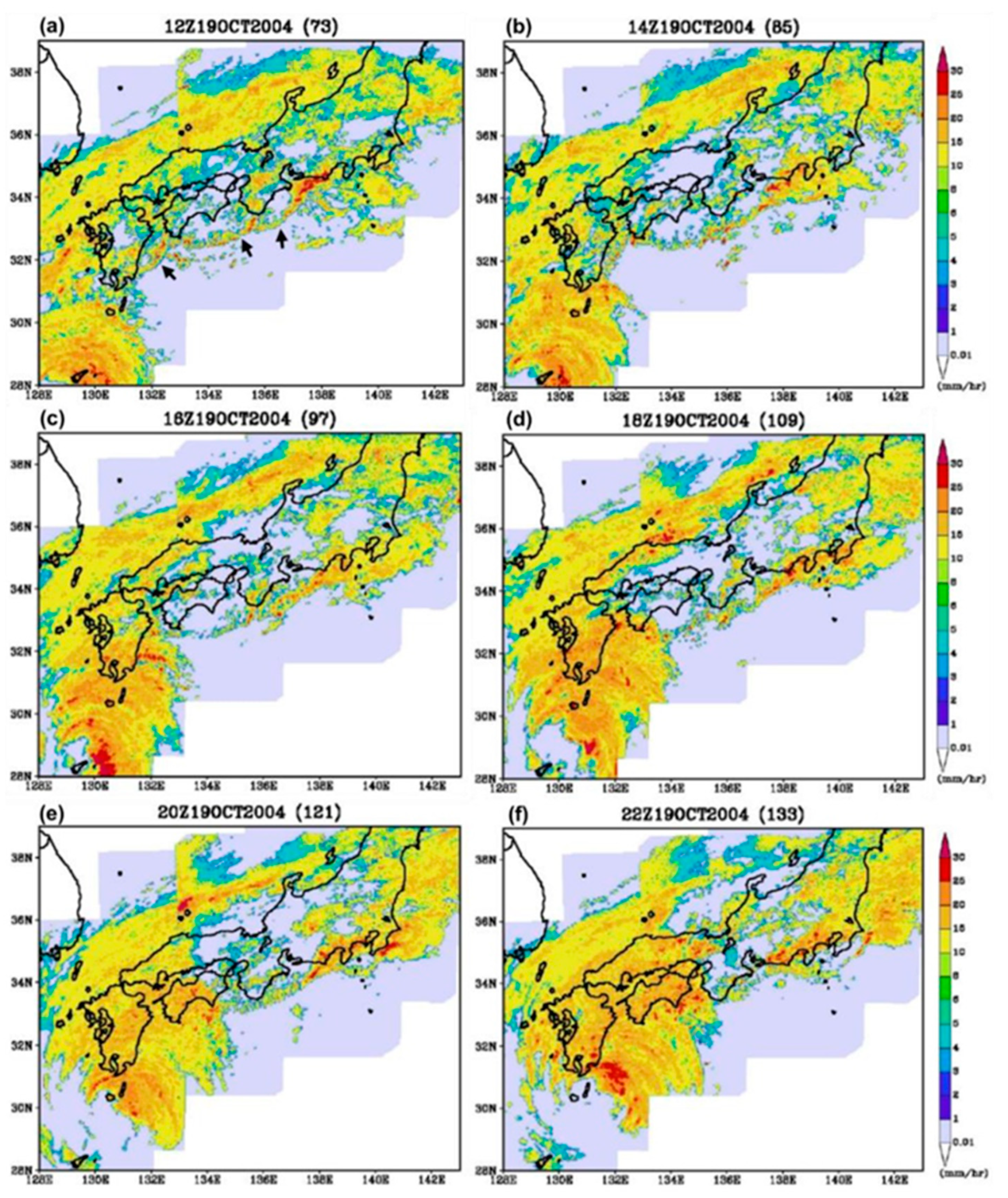
Figure 3 presents the rainfall intensity (or rain-rates) derived from the reflectivity of land-based radars operated by JMA at 2-h intervals from 1200 to 2200 UTC 19 October, and the rainbands can be clearly identified. Just prior to 1200 UTC, a series of spectacular arc-shaped rainbands (marked by arrows, Figure 3a) developed about 75–125 km to the south or southeast of the Japan isle, including Kyushu, Shikoku, and southern Honshu, when the center of Tokage was still between Okinawa and Amami Oshima (cf. Figure 1a). With bulges facing south to southeast, these narrow rainbands formed upstream from the island chain of Japan against the low-level southerly flow of the TC, with presumably northerly flow behind. Thus, they were aligned roughly parallel to the topography, and marked the location of the surface front at mesoscale (cf. Figure 2a,b). Meanwhile, another ENE–SSW-oriented, broader, but generally weaker rain belt just off the northern shore of Japan corresponded quite well with the wind-shift line and convergence near 700 hPa (cf. Figure 2c). The series of rainbands remained stationary for several hours, then collapsed and retreated (or washed) backwards one by one in succession when TY Tokage moved closer.
Taking place prior to 1600 UTC, the rainband upstream from Kyushu was the first one to collapse (Figure 3c). The one south of Shikoku retreated near 1900 UTC (Figure 3d,e), followed by the one south of Kii Peninsula near 2100 UTC (Figure 1b and Figure 3e,f). Hence, these rainbands retreated when the low-level southerly flow associated with TY Tokage became too strong and Fr increased, and this evolution in general corresponded to a shift from regime II to regime IV of CL05. The present case, therefore, provides a unique opportunity to examine the behavior of rainbands in association with island terrain during the transition from a relatively low-Fr to a high-Fr regime. In this study, we perform 3D cloud-resolving simulations with full physics to reproduce the event and utilize the model results to examine the behavior of the rainbands in response to the strengthening of oncoming flow, and the underlying mechanism(s) involved in this process.
3. The CReSS Model and the Experiment
The Cloud-Resolving Storm Simulator (CReSS) of Nagoya University [43,44] was used to simulate the development and evolution of the rainbands in the present case. Being both nonhydrostatic and compressible, the CReSS model is designed to simulate mesoscale weather systems realistically at high resolution, using explicit cloud microphysics without any cumulus parameterization. In the horizontal and vertical directions, the Cartesian and terrain-following curvilinear coordinates (based on height) are used, respectively, with the Arakawa-C staggering and Lorenz grid structures [43]. Prognostic equations for 3D momentum (u, v, w), pressure (p), potential temperature (θ), and mixing ratios of water vapor (qv) and other hydrometeors (qx, where x denotes a species) are formulated. The explicit bulk cold-rain scheme of CReSS is developed based on [45,46,47,48,49], with a total of six species (water vapor, cloud water, cloud ice, rain, snow, and graupel). The microphysical processes of nucleation (condensation), sublimation, evaporation, deposition, freezing, melting, falling, conversion, collection, aggregation, and liquid shedding are included (Table 1). The subgrid-scale turbulent mixing is parameterized using a 1.5-order closure with turbulent kinetic energy (TKE) prediction [44], while planetary boundary layer (PBL) processes are parameterized following [50,51]. Momentum and energy fluxes and radiation at the surface are also considered with a substrate model [51,52,53], but cloud radiation is neglected.
Since the model equation set includes all types of waves, a time-splitting scheme [54] is adopted for computational efficiency. The leapfrog scheme with the Asselin filter [55] is used for integration at large time steps (∆t), while the implicit Crank–Nicolson scheme is used at small time steps (∆τ) in the vertical. The Message Passing Interface (MPI) and/or Open MP are used for parallel computing. For a complete description of the formulation and different configurations and options of the CReSS model, the readers are referred to [43,56]. The CReSS model has been applied to successfully simulate a number of atmospheric phenomena, including winter cloud streets [57], convective lines due to terrain blocking of Taiwan during the Mei-yu season [10,36], and several typhoon cases [58,59,60]. In this work, we will investigate the formation and behavior of the arc-shaped convective lines during the approach of TY Tokage, as reviewed in Section 2, using the CReSS model. To our knowledge, such an investigation on the evolution of rainbands from a low- to a high-Fr regime has never been reported in the open literature.
For the present study, a single domain at 1-km horizontal grid spacing is used with a grid dimension of 1536 × 1408 × 60 (Figure 4), as the CReSS model has no nesting function. The simulation was carried out on the Earth Simulator using 1024 cores. The JMA regional analyses at 20-km and 6-h resolutions (with 21 levels from surface to 10 hPa) were used as initial and boundary conditions (IC/BCs), and real terrain (at roughly 1-km resolution) and sea surface temperature (SST) analysis by the JMA were provided. The simulation started from 1200 UTC 19 October 2004 for a duration of 30 h (until 1800 UTC 20 October), using 3 (1) s for ∆t (∆τ). No data nudging in the interior of the model domain was employed once the forward integration began. The major aspects in the configuration of the model and experiment are summarized in Table 1.
4. Model Results
4.1. Validation of CReSS Model Simulation
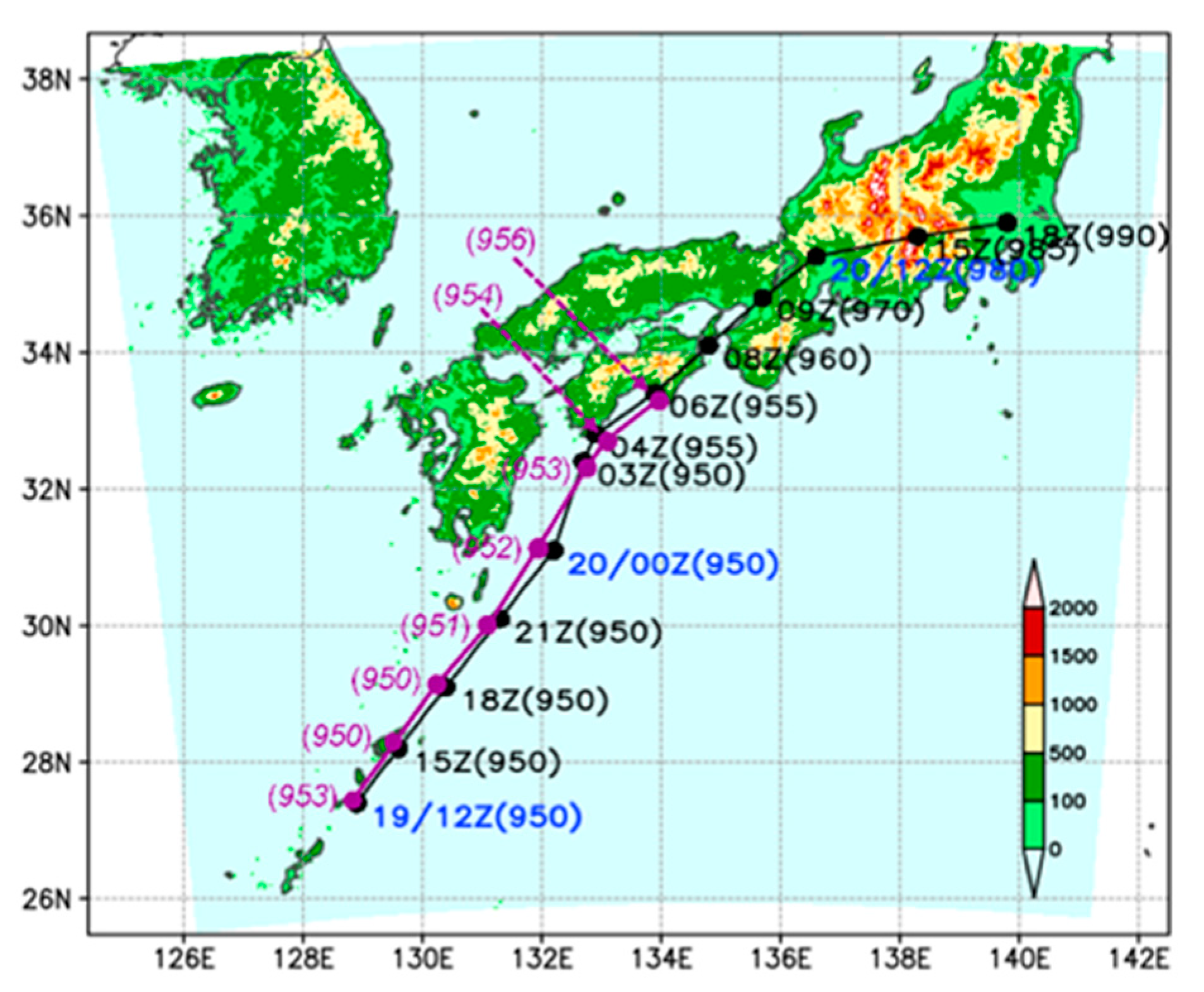
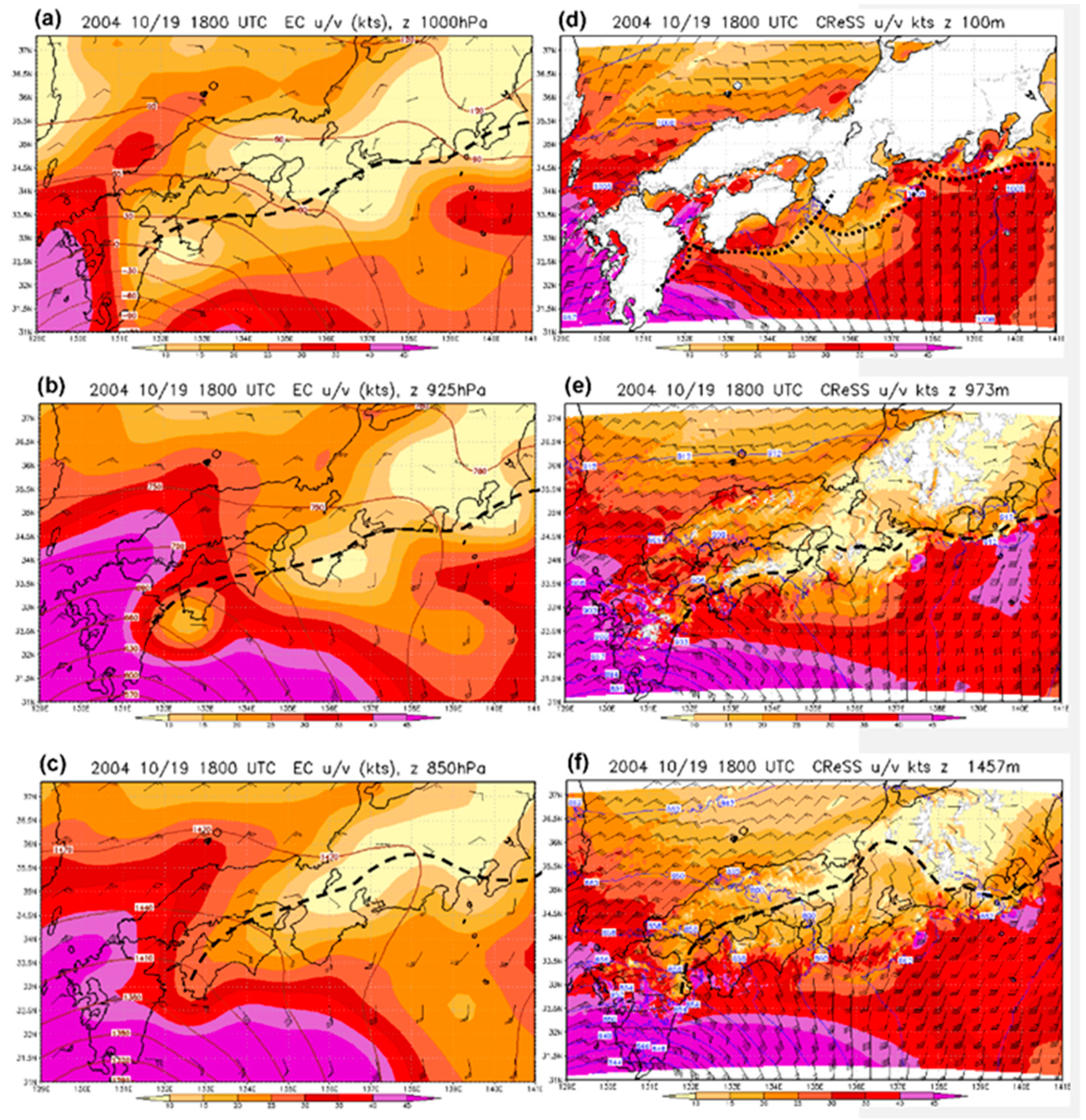
For the period when the arc-shaped rainbands existed, the simulated track of TY Tokage by the CReSS model is very close to the JMA best-track data, with a position error of no more than 50 km at most, while the central MSLP also agreed to within 3 hPa (Figure 4). To further validate the simulation surrounding western and central Japan, Figure 5 compares the model results at low levels with the gridded analyses (at 1.125° resolution) from the European Center for Medium-Range Weather Forecasts (ECMWF) at 1800 UTC 19 October, i.e., 6 h into the simulation.
Near the surface at 1000 and 925 hPa, the flow patterns in the ECMWF analysis are in good agreement with the weather maps (cf. Figure 2a,b,d,e), and the frontal zone/wind-shift line was near the southern shorelines of the Japan Isle (Figure 5a,b). On the other hand, in Figure 5c, the 850-hPa wind-shift line was located about 100 km farther north over the interior of Japan (north of Shikoku)—also consistent with Figure 2c,f. At levels near 925 and 850 hPa (at 973 and 1457 m, respectively), the model-simulated locations of the wind-shift line and the associated flow patterns in the region at 1800 UTC, with southerly (easterly to northeasterly) winds ahead or to its south (behind or to its north), are in close agreement with the ECMWF analysis (Figure 5e,f). At the lowest level of 100 m, the simulated near-surface flow contains considerably more details than the ECMWF analysis at 1000 hPa due to the fine resolution of the model (Figure 5d), and a series of narrow arc-shaped convergence/confluence zone (i.e., the mesoscale front) appear about 100 km upstream from the Japanese isles, in agreement with the observed rainbands in Figure 3. The easterly and northeasterly winds behind the bulging rainbands (to be discussed shortly) are well reproduced in Figure 5d and have been present in the model (as well as in the JMA regional analysis) since the beginning of the simulation at 1200 UTC 19 October (not shown). While the deceleration of the southerly flow upstream from the rainbands is evident in Figure 5d, the model wind speeds are stronger than those in the analyses (by about 5–10 kts) in some regions, such as the open ocean southeast of the Kii Peninsula (also at 973 and 1457 m) and near the TC center (cf. Figure 5a).
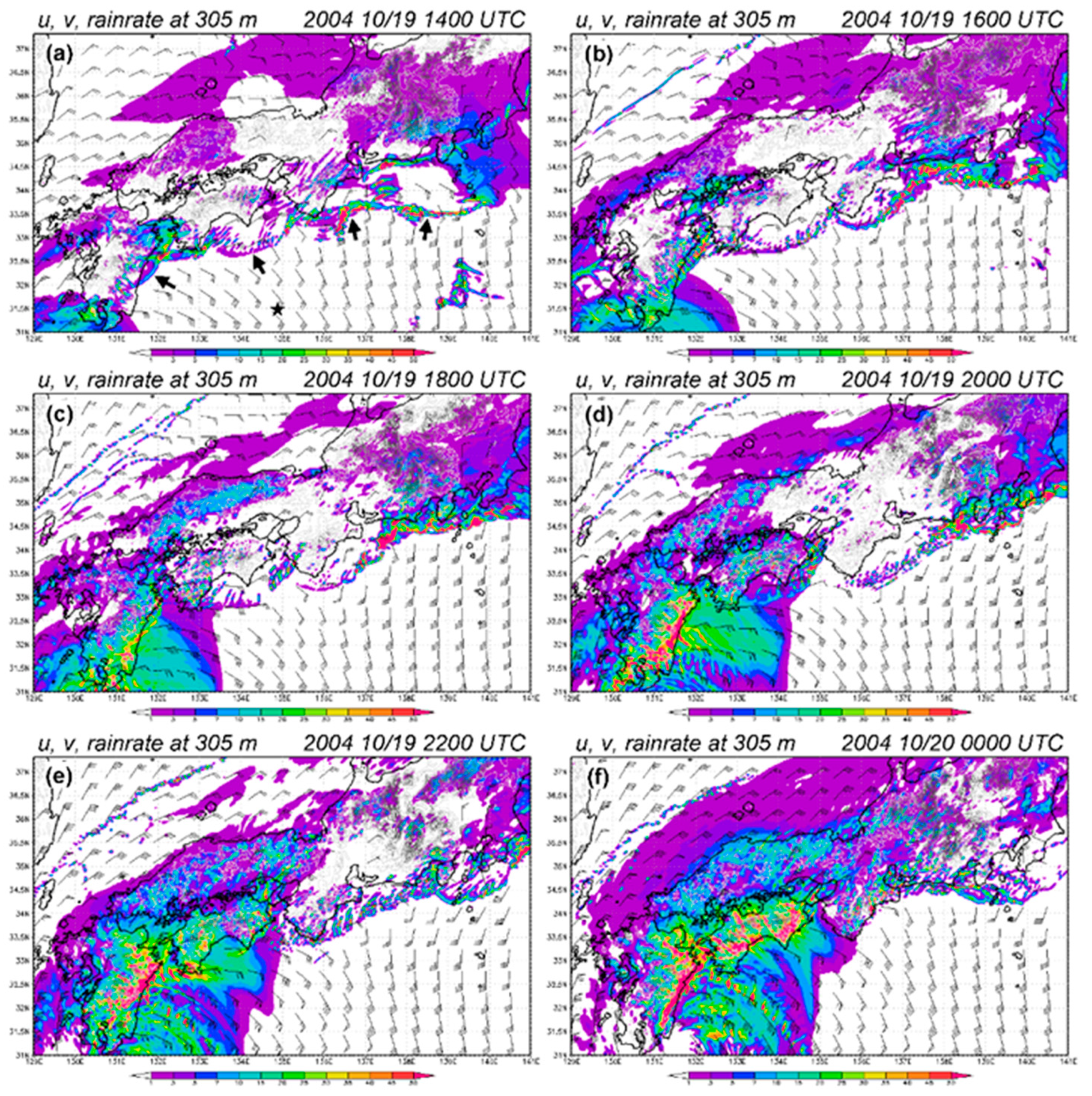
The model-simulated wind fields at 305 m and rainfall rates over the period of 1400–2400 UTC 19 October are shown in Figure 6 and can be compared with Figure 3 and Figure 5. In Figure 6, the gradual enhancement of the near-surface southerly flow upstream from the Japanese isles with time is well-captured, as confirmed through a comparison with ECMWF analyses during our case period (not shown). About one hour into the simulation (near 1300 UTC, not shown), a series of three to four arc-shaped rainbands developed just south of the Japanese isles, about 50–100 km upstream from Kyushu, Shikoku, and southern Honshu, and become well-defined before 1400 UTC (Figure 6a). During the following hours, the location, orientation, structure, and evolution of these rainbands with time in the model (Figure 6) are highly realistic and in close agreement with radar observations (Figure 3). While these rainbands are undoubtedly collocated with the narrow convergence zones near the surface, as discussed earlier (Figure 5d and Figure 6c), the model clearly well-captures the phenomenon of the collapse and retreat of the rainbands back over land (Figure 6). The retreat takes place around 1800 UTC for the one east of Kyushu, prior to 2000 UTC for the one south of Shikoku, and near 2100 UTC for the one upstream of Kii Peninsula in the model (Figure 6b–f), also highly consistent with Figure 3. Except for the arc-shaped rainbands, the rainfall distributions near the TC, off the northern shores of Japan, and over Chugoku (cf. Figure 1b) are all simulated quite well (Figure 6). In particular, note also that the narrow rainbands over the Japan Sea during 1400–2400 UTC in the model are observed as well (Figure 3 and Figure 6).
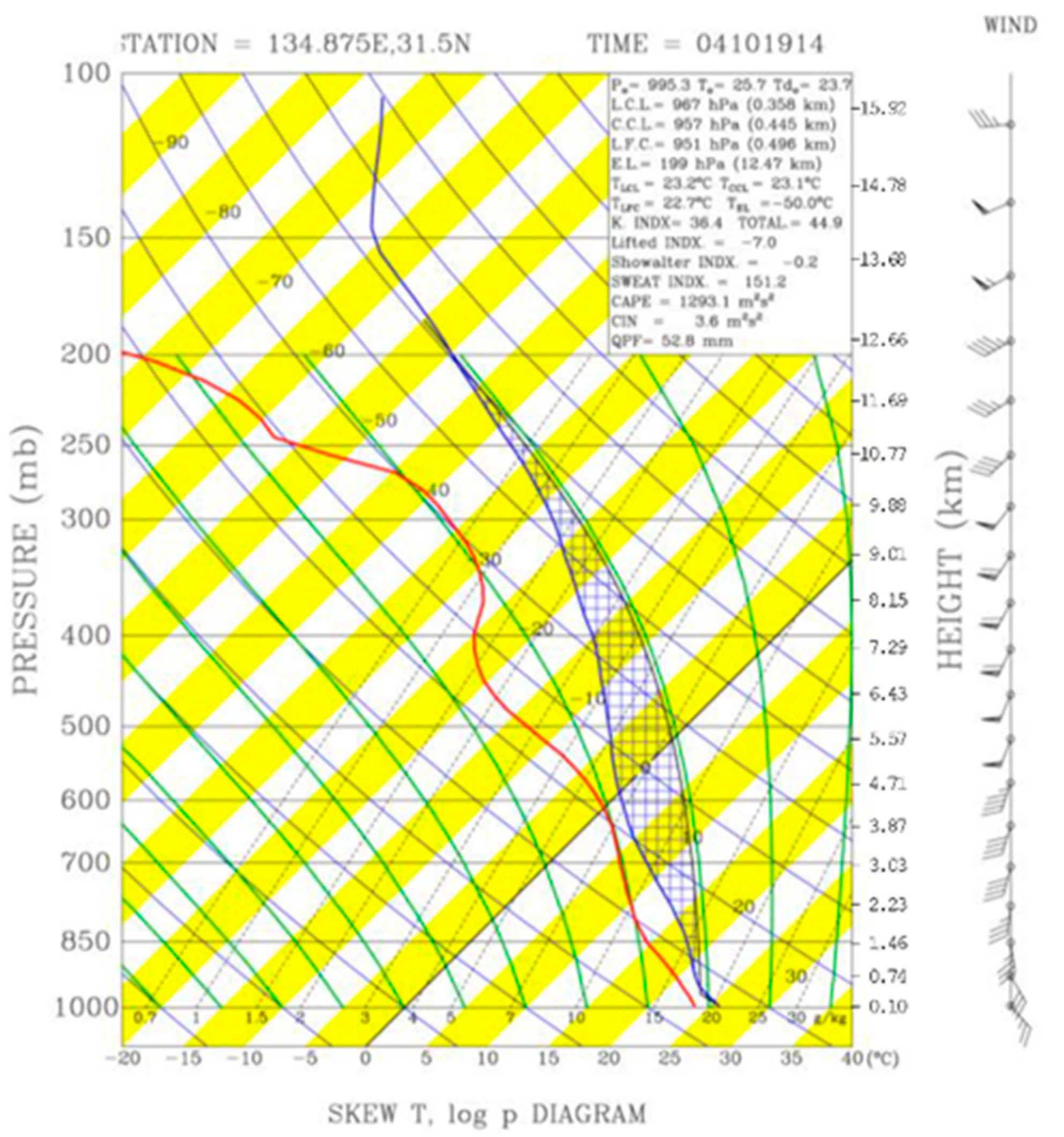
At the initial time of 1200 UTC 19 October 2004, the thermodynamic profile at 31.5° N, 134.875° E (marked by an asterisk in Figure 6a), i.e., about 130 km upstream from the rainband south of Shikoku, essentially from the JMA regional analysis indicates conditional instability for a surface air parcel, with a CAPE of 900 J kg−1 and negligible convective inhibition (CIN, 11 J kg−1, not shown). Mainly due to a gradual moistening of near-surface air over the ocean, the CAPE value increases to a maximum of about 1300 J kg−1 at 1400 UTC in the simulation, while the overall thermodynamic profile remains little changed (Figure 7). Note that with such a CAPE, regimes II to IV are predicted to occur when Fr falls inside the ranges of about <0.3, 0.3–0.5, and >0.5 in CL05.
From the above-detailed comparison with the observations, it is confirmed that the CReSS model simulation reproduces the development and subsequent evolution of the arc-shaped rainbands upstream from the western to central Japan in our case very successfully with high realm. Therefore, the high-resolution model results will be utilized to further study the behavior and retreat of these rainbands below in the following sections.
4.2. Rainband Behavior and Cross-Section Analysis
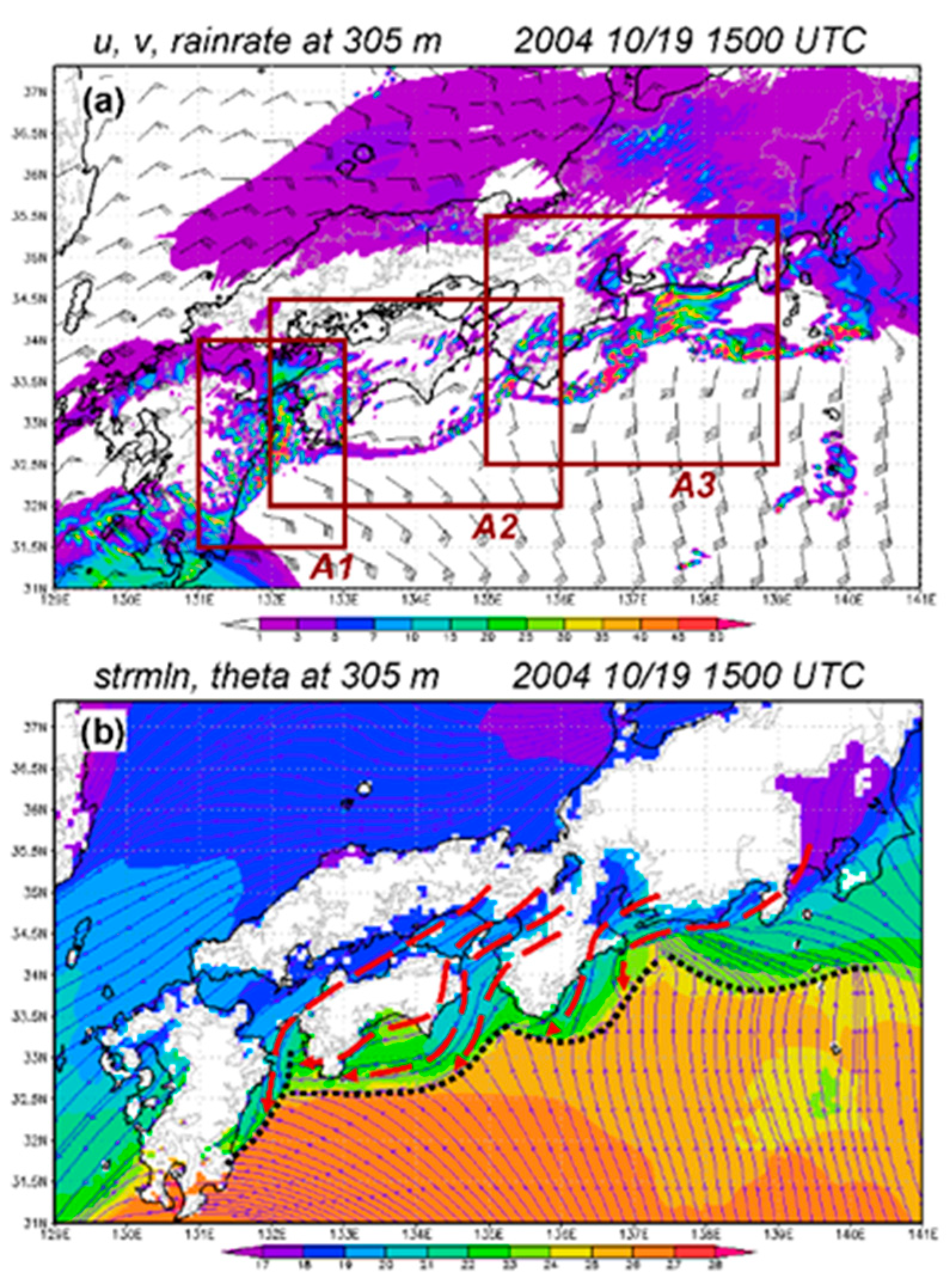
Figure 8 shows the model-simulated rain-rates along with 305-m winds as in Figure 6, except for 1500 UTC 19 October 2004 when the rainbands remained stationary. At this level, the clear convergence/confluence zones produced when the warm southerly flow of the TC circulation encountered the cold northeasterly flow (and southeasterly flow upstream from central Honshu, cf. Figure 1b) coincide with the rainbands (Figure 8a,b). While the potential temperatures (θ) of the upstream flow are at least 26 °C near 31° N, they are close to or below 20 °C in the northeasterly flow near the shorelines of Japan, and the thermal contrasts are roughly 2–4 K within a distance of 10–20 km across the rainbands (Figure 8b). For further examination, rectangular areas named Area 1 (A1), Area 2 (A2), and Area 3 (A3) are identified to enclose the individual rainbands upstream from Kyushu, Shikoku, and the Kii Peninsula, respectively (Figure 1b and Figure 8a), and a number of vertical cross-sections (VCSs) through these rainbands are constructed. From Figure 8b, note that the northeasterly flow from the Japan Sea cannot reach the back side of the rainbands in A1 and A2 without climbing over some topography and then sinking along the slopes. Also, a fourth rainband appeared farther east and upstream from the Japanese Alps of Honshu at 1500 UTC (Figure 8a,b), but it is not analyzed in the present study.
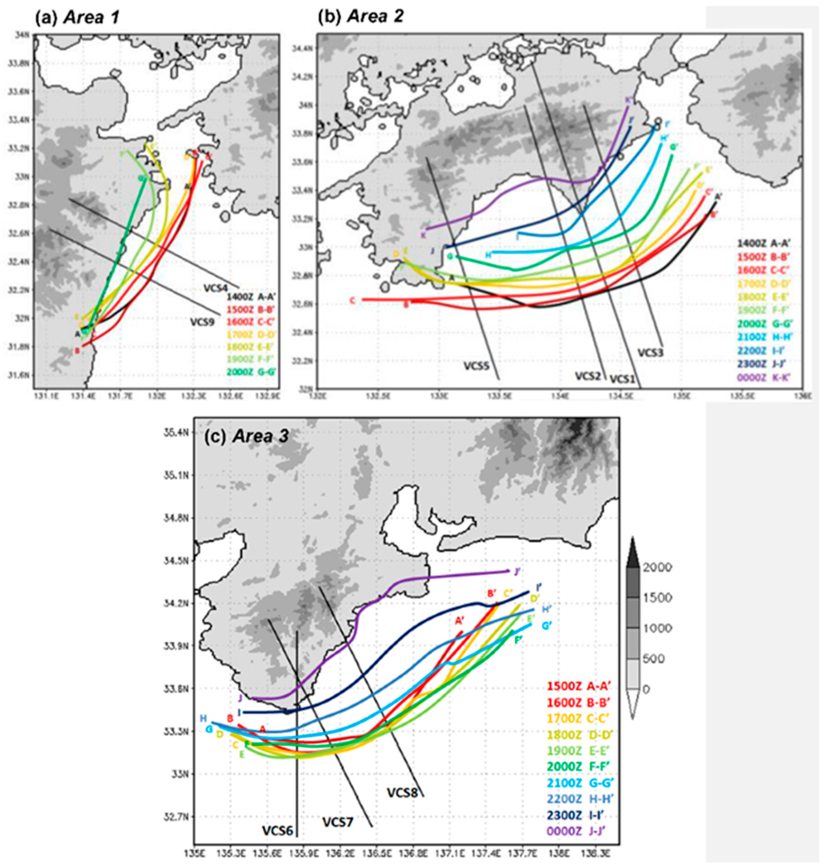
The temporal evolutions of the rainbands in the three areas are shown in Figure 9, which also depicts the locations of the VCSs constructed in this study, labeled as VCS1 through VCS9. The VCSs were selected to be roughly perpendicular to the rainbands. Using Figure 9, the three arc-shaped rainbands are traced through time (at 1-h intervals), and their behavior along each VCS is classified into three phases: standing (stationary or nearly so), retreating, and retreating back to land, as summarized in Table 2. Here, the standing phase is defined as the period when the rainbands remain stationary or nearly so. When the rainbands exhibit distinctly faster backward movement, it is defined as the retreating period, either over the ocean or back to over land. For the rainband upstream from Kyushu (in A1, Figure 9a), its southern segment apparently retreats earlier than the northern part. For the one upstream of Shikoku (in A2, Figure 9b), the retreat occurs around 1800–1900 UTC, but seems slightly earlier in the central segment than near the two ends. For the third rainband south of Kii Peninsula (in A3, Figure 9c), the retreat appears to occur concurrently along much of its length and shortly after 2000 UTC. In Table 2, the characteristic terrain height (h0) for each rainband (or area) is also given, which is estimated using Figure 9b and used for the calculation of Fr to be presented shortly.
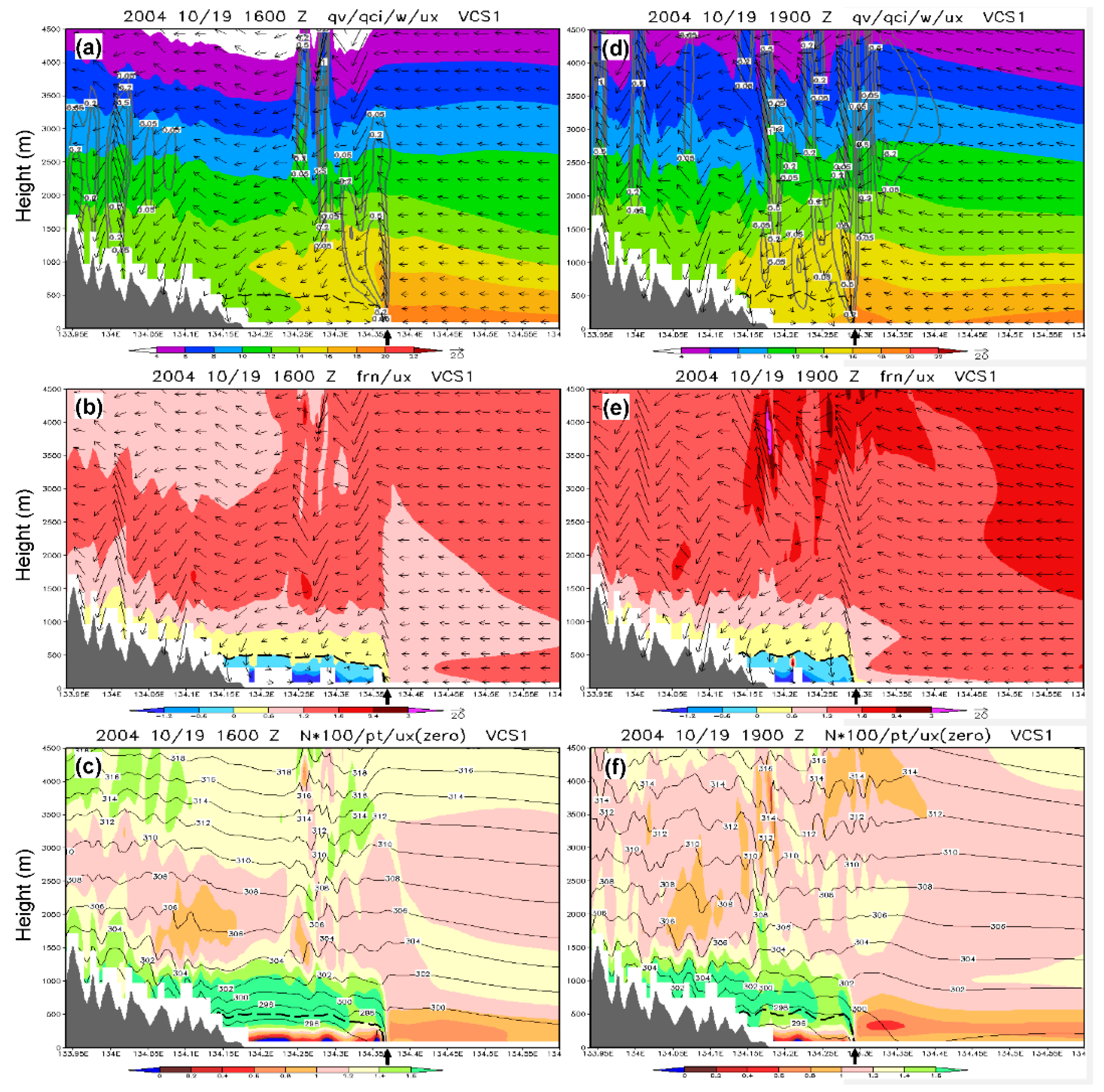
Although all vertical cross-sections were examined, only two of them, i.e., VCS1 in A2 and VCS7 in A3, are chosen here for presentation and detailed analysis following this order (Figure 10 and Figure 11). In Figure 10, the evolution of the rainband and its surrounding environment along VCS1 in A2 (about 183 km in length), at 1600 and 1900 UTC 19 October is shown (cf. Figure 9b). During the standing phase at 1600 UTC (Figure 10a–c), when the model rainband (thick arrow) remained near 134.37° E (and 32.78° N), the component of the upstream flow parallel to the section plane was quite uniform and about 10–20 m s−1 from the surface to 4 km and was able to penetrate through the rainband except near the surface (Figure 10a), in agreement with Figure 5. The opposing offshore flow was confined to below 500 m and quite shallow, and the component on the plane was only ≤5 m s−1 since the northeasterly flow, clearly from the post-frontal environment, intersected with VCS1 at a large angle (cf. Figure 6b and Figure 8b). On the other hand, clear downward motion at cloud scale also existed north of the rainband (and below the clouds) at low-to-middle levels and circulated and contributed to the offshore winds near the surface (Figure 10a). At 1–3 km, the upstream flow was dry, stable, and exhibited Fr values of near 1.4 (using h0 = 1.1 km, cf. Table 2), with N about 1.0–1.3 × 10⁻² s−1, which corresponds to dθ/dz of about 3–4 K km−1 (Figure 10b,c). Even before the retreat, such Fr values upstream were already significantly larger than those appeared in CL05. The offshore flow was about 3–4 K colder (and also drier) than the upstream onshore flow, and upward motion of >1 m s−1 was produced at its leading edge to generate the rainband (Figure 10c). Note that behind the rainband, the stability was particularly high (N ≈ 1.4–1.7 × 10⁻² s−1) from the upper part of the offshore layer to about 1.2 km (with smaller vertical spacing between isentropes), and smaller Fr resulted here in combination of weak onshore flow components.
Three hours later at 1900 UTC (Figure 10d–f), the upstream flow (on the section plane) strengthened to about 19–23 m s−1 and Fr also increased to roughly 1.8–2.4 at 1–3 km, and the rainband started to retreat (cf. Figure 9b and Table 2). Nonetheless, N remained nearly unchanged (Figure 10f), similar to the finding of [27] for Hawaii Island. Note also that at 1800 UTC a gap appeared in the rainband along its middle segment (near VCS1, cf. Figure 6c), and then the rainband started to retreat, apparently also faster in the middle part (cf. Figure 9b and Table 2). In Section 5.3, the possible linkages between the rainband gap and the retreat will be further discussed.
During later hours when the rainband continued to retreat to near the shoreline of Shikoku (cf. Figure 9b), the surface-based offshore flow vanished and only onshore flow existed along VCS1 (not shown). The upstream flow components and Fr at low levels continued to increase (to about 30–40 m s−1 and 2.5, respectively) and N also rose slightly, with the approach of TY Tokage, in agreement with Figure 4 and Figure 6e. After the collapse of the rainband, the low-level southerly flow from the TC could climb over the terrain in Shikoku with forced uplift in a high-Fr regime (not shown), and the rainfall over the slopes significantly increased (cf. Figure 6b–f).
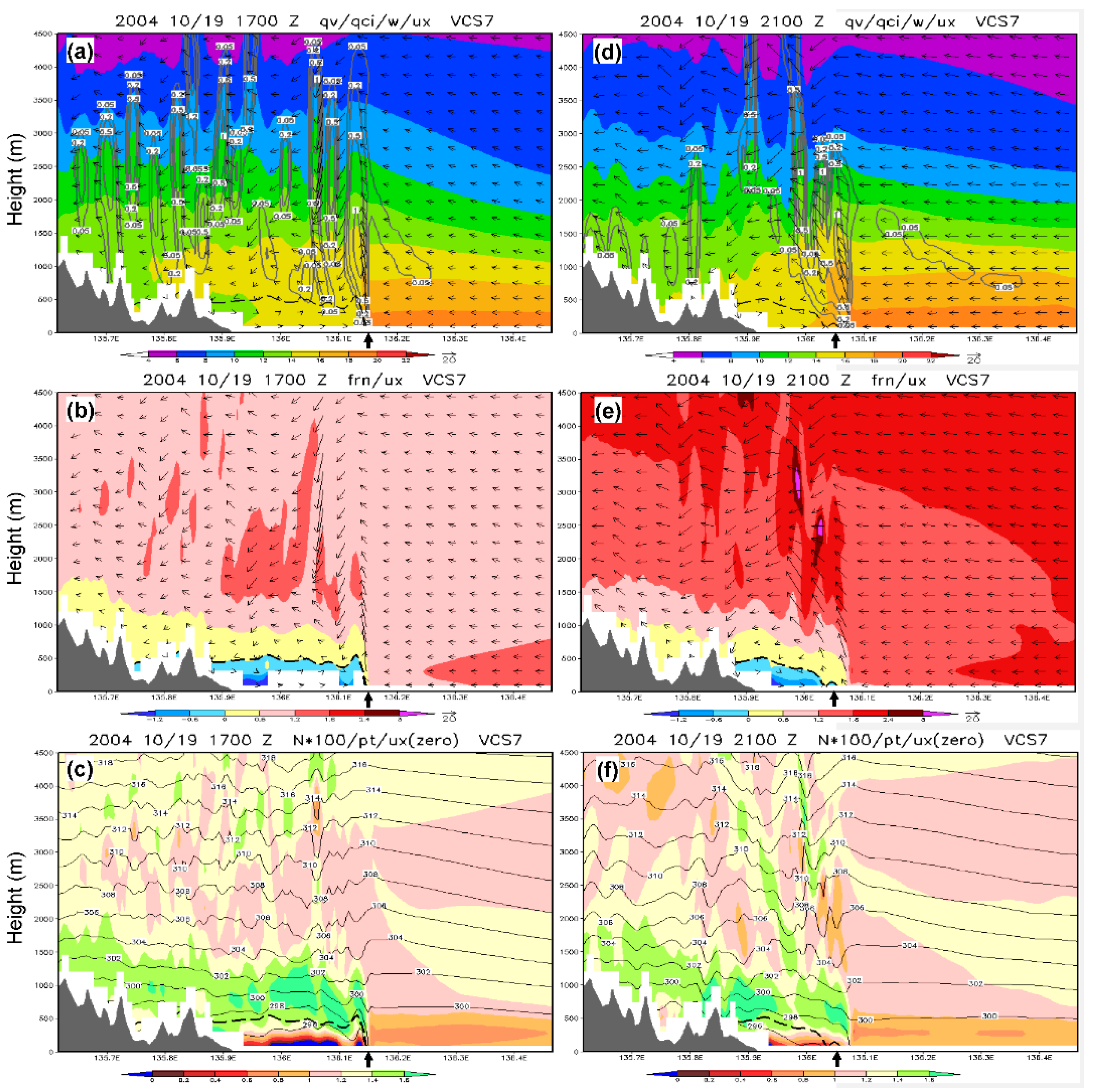
For A3, VCS7 was selected for two times, 1700 and 2100 UTC, as shown in Figure 11 (about 185 km in length). As this rainband was farther from the TC than that in A2, it was in the standing phase before 2000 UTC (Figure 11a–f) and retreating phase at 2100 UTC (Figure 11d–f), and retreated almost back to land at 2300 UTC (cf. Figure 9c). The overall evolution of the rainband along VCS7 was quite similar to that along VCS1 in A2, and the low-level upstream flow parallel to the section plane at 1–3 km increased gradually to about 10 m s−1 around 1700 UTC, raising Fr to about 1.2 with N ranging at 0.8–1.2 × 10⁻² s−1 (using h0 = 900 m, Figure 11a–c). The surface-based offshore flow behind the rainband only existed below 500 m and got thinner with time during the standing phase (not shown), and it was roughly 2–3 K colder than the onshore flow. Just above the offshore flow, the stability was again higher up to about 1.5 km, and the N values could reach >1.4 × 10⁻² s−1 at 1700 UTC (Figure 11c). From near-surface plots similar to (and including) Figure 8c, it is revealed that many of the cold regions behind the rainband during the standing phase possessed local minimum θ values, and hence must also have been contributed by (diabatic) cooling from the evaporation of precipitation below the clouds, in addition to purely (adiabatic) 3D advection. In Figure 10a–c and Figure 11a–c, the θ values in the offshore layer often tended to be lower below strong downdrafts. This is also indicative of evaporative cooling, which is obviously the main cause of the high stability in the upper part and just above the offshore layer in the VCSs (Figure 10c and Figure 11c).
After 1900 UTC, the model rainband along VCS7 showed a clearer sign of retreat (cf. Figure 9c and Table 2). This weakening of rainband and offshore flow, also seen at 1800 UTC along VCS1 (not shown), thus appears to be a common precursor to the retreat of rainbands in A2 and A3. During the retreating phase at 2100 UTC (Figure 11d–f), the oncoming low-level flow at 1–3 km became significantly stronger (about 20–25 m s−1), and Fr also increased to about 1.6–2.0 although N remains nearly unchanged. The rainband continued to be washed backward during this period and moved close to the shore of the Kii Peninsula at 2300 UTC (not shown), when the rainfall over the slopes also increased (cf. Figure 6c–f). This evolution when the rainband retreated back to land, with typically enhanced updrafts and downdrafts, is also reminiscent to that along VCS1 in A2.
For A1, which was closest to the TC, the VCSs were also examined (figure not shown). The offshore layer behind the rainband in A1 (e.g., along VCS9) was also about 500 m in depth (and about 3 K colder than the upstream flow) at 1400 UTC, but the offshore wind components are relatively weak because the environmental northeasterly flow, after traveling through the Seto Inner Sea, was blowing at small angles from behind, almost parallel to the rainband (cf. Figure 1b and Figure 8c). Compared to other VCSs (cf. Figure 10 and Figure 11), the stable layer above the offshore flow during the standing phase was even thicker and more stable (>1.6 × 10⁻² s−1) in A1 and remained so during the retreating phase (not shown). Note also that, being closer to the TC, the rainfall over the windward slopes of Kyushu in A1 was typically more intense than those associated with other rainbands (cf. Figure 6), in agreement with [14,35].
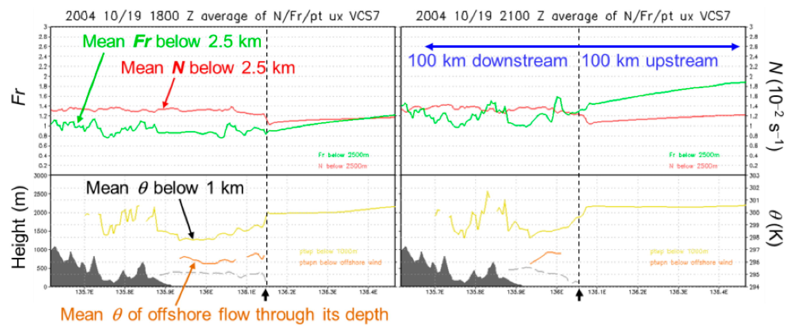
Several key parameters relevant to rainband behavior on the vertical cross-sections at low levels as shown in Figure 10 and Figure 11 can be averaged through appropriate depths (e.g., [61]), and the resulted distribution along the sections can be plotted and examined more easily, as shown for example in Figure 12 for VCS7. Values of Fr and N are averaged below 2.5 km to depict the mean properties in the upstream flow and their differences from those in the flow behind the rainband, while θ values are averaged below 1 km and also through the depth of the offshore flow only. At 1800 UTC, during the standing phase (Figure 12a), a time between those in Figure 11a–f, the mean N (of 0–2.5 km) was about 1.0–1.2 × 10⁻² s−1 ahead of, but higher (about 1.3–1.4 × 10⁻² s−1) and more stable behind the rainband. The mean Fr was about 0.9–1.2 upstream, and was comparable but much more variable downstream due to the stronger but more fluctuating wind components there (cf. Figure 11b,e). Corresponding to higher N values, the near-surface mean θ (of 0–1 km) was about 2 K colder behind than ahead of the rainband due to evaporative cooling effect, as discussed earlier, and the mean value in the offshore layer (≤500 m) was typically another 2–2.5 K colder (Figure 12a). At 2100 UTC during the retreating phase (Figure 12b, same time as Figure 11d–f), the upstream Fr increased significantly to about 1.4–1.9 but N changed little both upstream and downstream. Although the θ values below 1 km and in the offshore layer remained colder, the thermal contrast at the leading edge of the offshore flow, where it became very thin, was reduced (Figure 12b) as the rainband was pushed backward by the strengthening oncoming flow.
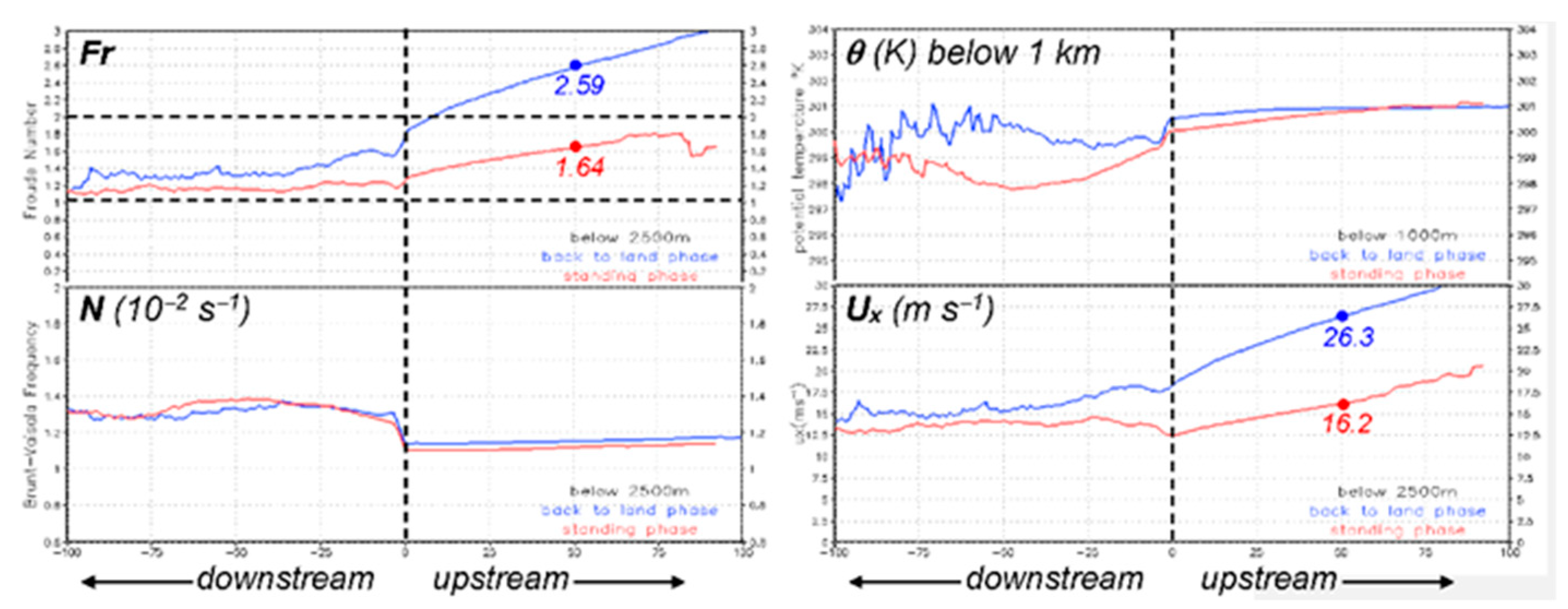
Using the location of the rainband as a common reference point, results similar to Figure 12 at different times and along different VCSs can be further composited into those for A1, A2, and A3, respectively. One such example is shown in Figure 13 for the standing phase (red) and the phase of retreating back to land (blue). Here, all variables are averaged below 2.5 km, except for θ, which is averaged below 1 km as in Figure 12, and in the discussion, we will emphasize the changes in the characteristics from the low-Fr to high-Fr regime between the two phases. As seen, the upstream low-level flow speed and Fr (below 2.5 km) increased during the approach of TY Tokage, and we use the values at 50 km ahead of the rainband for easy comparison. In the standing phase, the mean wind component parallel to section (Ux) was 16.2 m s−1 in A2, yielding a Fr of 1.64 (red dots, Figure 13). When the rainbands retreated back over land, the mean Ux enhanced to 26.3 m s−1 and Fr also increased to 2.59 (blue dots). Behind the rainband, the differences in Fr and Ux between the two phases are much smaller. In the standing phase, the mean θ values (below 1 km) were at most roughly 3 K colder and N about 0.3 × 10⁻² s−1 higher behind the rainband than ahead of it. When the rainbands retreated back to land, N remained little changed at both sides of the rainband, while the mean θ downstream increased (Figure 13), most significantly in A2, likely linked to the longer time period separating the two phases (cf. Table 2).
5. Discussion
5.1. Comparison to Idealized 2D Simulation Results
In plots for all three areas including Figure 13, the Fr values upstream from the rainbands were roughly 1.2–2.1 during standing phase and above 2.1 during the phase back over land in the present case. While the behavior of rainbands generally corresponds to a transition from regime II to IV of CL05, the Fr values in our case are significantly higher than those of about 0.1–1.0 obtained from idealized 2D studies (also [24]). Since the low-level flow was horizontally uniform at the initial time in the 2D simulations, one major difference in our case is obviously the existence of the low-level northeasterly offshore flow behind the rainbands from the environment (cf. Figure 6 and Figure 8c). In other words, the rainbands in our case developed when two nearly opposing airflows encountered each other along the front (or wind-shift line) roughly parallel to the topography of Japan at low levels (Figure 2 and Figure 8c), and this three-dimensionality with more complicated flow structure in the background (and one more degree of freedom) was not included in those previous 2D experiments (e.g., [20,24]; CL05). Thus, the existence of the offshore flow from the northeast or east, against the oncoming flow from the south, allowed the rainband to remain stationary under much higher upstream wind speed and Fr values. When the Fr continued to increase as TY Tokage moved closer, on the other hand, the retreat and collapse of the rainbands (Figure 3 and Figure 6) were consistent with the behavior predicted by the 2D results from low- to high-Fr regimes.
In our case, even though the rainbands were not produced directly by terrain blocking under a more-or-less uniform prevailing flow (as in the idealized 2D studies), their location and shape still appeared to be closely tied to the topography. The series of rainbands formed about 75–125 km upstream from the islands of Kyushu and Shikoku, and Kii Peninsula and the Japanese Alps in Honshu, respectively, and remained stationary for hours before their retreat (Figure 1b, Figure 3 and Figure 6). This was because the low-level northeasterly flow needed to pass through the gaps between higher terrain (i.e., Bungo Channel, Kii Channel, and the Seto Inner Sea) to reach the backside of rainbands, and this process and the associated wind speed enhancement through the channel effect are also visible in our simulation (Figure 6 and Figure 8c). Thus, the rainbands in this study naturally appeared and bulged southward (or southeastward) upstream from the mountainous regions in southwestern Japan. Compared to the rainband locations found in earlier studies (e.g., [40,41]), those in the present case also appeared farther upstream relative to the local terrain.
5.2. Comparison among Different Cross-Sections in the Three Areas
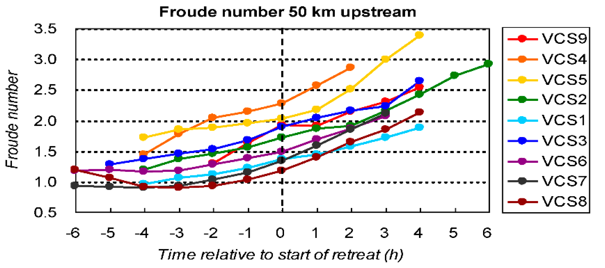
In this subsection, the behavior of the rainbands during the transition from low- to high-Fr regime is further compared among different VCSs in the three areas. From plots similar to Figure 12, the changes in the averaged Fr (below 2.5 km) 50-km upstream from the rainbands with time along all nine VCSs are obtained and plotted in Figure 14, using the time to start retreating as a common reference point. While the increase in Fr leading to the retreat is clear in all VCSs, the Fr values at the commencement of retreat varies considerably among the VCSs and in different areas although they are all at least about 1.2 (Figure 14). In A3, which was farther away from the TC, (VCS6 to VCS8), the rainband started to retreat when Fr reached relatively low values of 1.2–1.5 compared to A1 and A2. Although Fr might be slightly underestimated for VCS7 and VCS8 because they were less parallel to the upstream flow, part of the reason is also likely that the low-level offshore wind behind the rainband in A3 was from the easterly flow to the south of the Japanese Alps instead of from the Japan Sea, and thus is weaker (cf. Figure 6, Figure 8 and Figure 9c). In Figure 14c, the mean deficit in θ behind the rainband from the upstream values in A3 also appears smaller than those in other two areas. On the other hand, VCS4 in A1 did not start retreating until the Fr exceeded 2.25, which is significantly higher than the Fr of about 1.9 for VCS9 to the south. While Fr in A1 tended to be high due to its close proximity to the TC, the rainband along VCS4 was close to the terrain of Kyushu and the low-level flow behind it was from the Seto Inner Sea and passed through the narrow Bungo Channel (cf. Figure 1b and Figure 6c). As discussed earlier, the mean θ deficit across the rainband in A1 was also the largest among the three areas (Figure 13a). For the VCSs in A2, the Fr values at the beginning of the retreat fell into the middle range of about 1.4–2.0 (Figure 14).
5.3. The Role of Evaporative Cooling in Offshore Flow
From the analysis in Section 4.2, it is revealed that the surface-based offshore flow (from the east or northeast) behind the rainbands, with a typical depth of 500 m, must have also been contributed by evaporative cooling of precipitation, in addition to (adiabatic) advection. The cooling tends to be stronger (with lower θ values) below strong downdrafts, and results in a highly stable layer below about 1.5 km (cf. Figure 10 and Figure 11). Trapped between the rainband and the terrain, the convectively-enhanced cold outflow acted like a density current and pushed against the oncoming flow from the south, and such a process is suggested to be important to help the convective system remain stationary against the mean flow by both [24] and CL05. Hence, in our case the arc-shaped rainbands were able to maintain their position for at least 2–3 h despite the gradual increase of Fr, until the oncoming winds became too strong (Figure 10a–f and Figure 11a–f). Once the rainbands started to retreat, however, the local cooling behind them could not accumulate in its effect and became less effective, and they were further washed back and collapsed. This is reflected in the thinner depth with higher θ values in the offshore flow (Figure 10 and Figure 11) and the smaller θ deficit across the rainband during the retreating phase, compared to the standing phase (Figure 12 and Figure 13), especially in A2. Recall our analysis in Section 4.2 that the rainband along VCS1 started its retreat shortly after 1800 UTC (Figure 9b and Figure 10d–f), when a gap appeared at its middle segment (cf. Figure 6c), inevitably causing a weakening in the evaporative cooling effect. Finally, when the three areas are compared, it is shown that the rainbands in A1 (upstream from Kyushu, VCSs 4 and 9) were able to maintain their positions under higher Fr values (up to 1.9) when θ values remained lower (stronger cooling) behind them (details not shown), while the rainband in A3 started to retreat under relatively low Fr values (≤1.5) when the θ deficit across the rainband was comparatively small (Figure 14, VCSs 6–8). Thus, all the above evidences do suggest that a role was played by evaporative cooling in helping rainbands to hold their position before the retreat, in agreement with [24], CL05, and several other previous studies (e.g., [62,63,64]).
6. Concluding Remarks
During 19–20 October 2004, a series of spectacular arc-shaped rainbands developed south of the isle and topograghy of southwestern Japan, including Kyushu, Shikoku, Kii Peninsula, and the Japanese Alps, when Typhoon Tokage (TY0423) approached the region from the southwest. Under a low-level prevailing flow from the south, these rainbands remained stationary for several hours, and eventually collapsed and retreated backward when the typhoon became too close and the Froude number (Fr) became too large. Therefore, this case provides a unique opportunity to examine the behavior of upstream rainbands associated with mesoscale orography during the transition from a relatively low-Fr to a high-Fr regime.
Using the Nagoya University CReSS model at a horizontal grid spacing of 1 km (with 40 levels), this event was successfully simulated and reproduced, with the location and evolution of rainbands highly reminiscent to those observed. A total of nine vertical cross-sections (VCSs) roughly perpendicular to the topography and through three rainbands were constructed for detailed examination on their structure and behavior during the period of interests, and the results are compared with those from idealized 2D simulations (e.g., [24]; CL05). The major findings are summarized below.
- (1).
- The rainbands developed as a result of low-level convergence along a frontal zone between the southerly flows associated with Typhoon Tokage and the northeasterly (or easterly) winds from the Sea of Japan. The northeasterly flow accelerated through gaps between topography and descended to feed the offshore flow toward the backside of the rainbands. This process dictated the bulged shape of rainbands and allowed them to form farther upstream, at about 75–125 km from mountain peaks.
- (2).
- Against the warmer upcoming southerly flow, the cooler offshore flow (with a θ deficit typically about 2–4 K) from the northeast or east also allowed the rainbands to remain stationary under significantly higher Fr values than predicted by 2D simulations, in which the background flow is uniform and the offshore flow is initially generated by terrain blocking. In the present case with a CAPE of about 1300 J kg-1, the rainbands remained quasi-stationary and did not start to retreat until Fr reached at least 1.2 or larger, while retreat typically occurs at a much lower range of 0.3–0.5 in previous 2D results.
- (3).
- During the transition from standing to retreating phase of rainbands, the wind speed and Fr of the low-level upstream flow increased significantly but the stability (i.e., buoyancy oscillation frequency) remained little-changed. Consistent with earlier studies, the shallow surface-based offshore flow (typically about 500 m in depth), like a density current, was enhanced by evaporative cooling of precipitation behind the rainbands besides (adiabatic) advection. The cooling effect led to a highly stable layer below about 1.5 km behind the rainbands and allowed them to hold their position for at least 2–3 h before retreat, despite the gradual increase of upstream Fr in our case.
- (4).
- Once the oncoming winds became too strong and Fr became too large, and the rainbands started to retreat and collapsed. At this stage, local cooling behind them was less effective, and the offshore layer became thinner and the θ deficit from the upstream flow also reduced. Closest to the TC, the rainband southeast of Kyushu (in Area 1) did not start to retreat until Fr exceeded at least 1.9 due to stronger northeasterly flow and evaporative cooling. On the contrary, the rainband south of the Kii Peninsula (in Area 3), farther from Tokage, was associated with a smaller θ deficit, and its retreat began when Fr reached 1.2–1.5.
Author Contributions
Conceptualization, C.-C.W. and K.T.; Data curation, C.-C.W., T.-C.L. and K.T.; Formal analysis, T.-C.L. and Y.-M.T.; Funding acquisition, C.-C.W. and D.-I.L.; Investigation, C.-C.W., T.-C.L. and K.T.; Methodology, C.-C.W., T.-C.L., K.T. and D.-I.L.; Project administration, C.-C.W.; Resources, C.-C.W. and K.T.; Software, T.-C.L. and K.T.; Supervision, C.-C.W.; Validation, K.T.; Visualization, T.-C.L. and K.T.; Writing—original draft, C.-C.W., T.-C.L. and Y.-M.T.; Writing—review and editing, all authors. All authors have read and agreed to the published version of the manuscript.
Funding
This study was supported by the Ministry of Science and Technology (MOST) of Taiwan (grants: NSC-99-2111-M-003-004-MY3, MOST-108-2111-M-003-005-MY2, and MOST-110-2111-M-003-004) and by the National Typhoon Center/Korea Meteorological Administration (KMA) under “Development of Typhoon Analysis and Forecast Technology” (grant: KMA2018-00722).
Data Availability Statement
The CReSS model and its user’s guide are available at http://www.rain.hyarc.nagoya-u.ac.jp/~tsuboki/cress_html/index_cress_eng.html accessed on 23 September 2021, and the RSM regional analyses available from the JMA. The basic model setting is given in Table 1 and the details are available from the authors (C.-C.W. and K.T.).
Acknowledgments
The authors wish to thank the two anonymous reviewers and Hung-Chi Kuo of National Taiwan University for their helpful comments, Atsushi Sakakibara for his help to perform the simulation experiment, and the assistance from Shin-Yi Huang and Yi-Wen Wang. The best-track and radar data used in Figure 3 and Figure 4 and the regional analysis using as IC/BCs of our simulation are provided by the JMA.
Conflicts of Interest
The authors declare no conflict of interest.
References
- Smith, R.B. The influence of mountains on the atmosphere. Adv. Geophys. 1979, 21, 87–230. [Google Scholar]
- Rotunno, R.; Klemp, J.B.; Weisman, M.L. A theory for strong, long-lived squall line. J. Atmos. Sci. 1988, 45, 463–485. [Google Scholar] [CrossRef] [Green Version]
- Smolarkiewicz, P.K.; Rasmussen, R.; Clark, T.L. On the dynamics of Hawaiian cloud band: Island forcing. J. Atmos. Sci. 1988, 45, 1872–1905. [Google Scholar] [CrossRef] [Green Version]
- Browning, K.A. Organization of Clouds and Precipitation in Extratropical Cyclones. In Extratropical Cyclones; Newton, C.W., Holopainen, E.O., Eds.; American Meteorological Society: Boston, MA, USA, 1990; pp. 129–1533. [Google Scholar]
- Houze, R.A., Jr. Cloud Dynamics; Academic Press: San Diego, CA, USA, 1993; p. 570. [Google Scholar]
- Kingsmill, D.E. Convection initiation associated with a sea-breeze front, a gustfront, and their collision. Mon. Weather Rev. 1995, 123, 2913–2933. [Google Scholar] [CrossRef] [Green Version]
- LeMone, M.A.; Zipser, E.J.; Trier, S.B. The role of environmental shear and thermodynamic conditions in determining the structure and evolution of mesoscale convective systems during TOGA COARE. J. Atmos. Sci. 1998, 55, 3493–3518. [Google Scholar] [CrossRef]
- Zhang, F.; Koch, S.E. Numerical simulations of a gravity wave event over CCOPE. Part II: Waves generated by an orographic density current. Mon. Weather Rev. 2000, 128, 2777–2796. [Google Scholar] [CrossRef]
- Schultz, D.M.; Knox, J.A. Banded convection caused by frontogenesis in a conditionally, symmetrically, and inertially unstable environment. Mon. Weather Rev. 2007, 135, 2095–2110. [Google Scholar] [CrossRef]
- Wang, C.-C.; Huang, W.-M. High-resolution simulation of a nocturnal narrow convective line off the southeastern coast of Taiwan in the mei-yu season. Geophys. Res. Lett. 2009, 36, L06815. [Google Scholar] [CrossRef] [Green Version]
- Pierrehumbert, R.T.; Wyman, B. Upstream effects of mesoscale mountains. J. Atmos. Sci. 1985, 42, 977–1003. [Google Scholar] [CrossRef] [Green Version]
- Banta, R.M.; Berri, G.; Blumen, W.; Carruthers, D.J.; Dalu, G.A.; Durran, D.R.; Egger, J.; Garratt, J.R.; Hanna, S.R.; Hunt, J.C.R.; et al. Atmospheric Processes over Complex Terrain; Meteor Monogr: Park City, UT, USA, 1990; p. 323. [Google Scholar]
- Baines, P.G. Topographic Effects in Stratified Flows; Cambridge University Press: Cambridge, UK, 1995; p. 482. [Google Scholar]
- Rotunno, R.; Ferretti, R. Orographic effects on rainfall in MAP cases IOP 2b and IOP 8. Q. J. R. Meteor. Soc. 2003, 129, 373–390. [Google Scholar] [CrossRef]
- Medina, S.; Houze, R.A., Jr. Air motions and precipitation growth in alpine storms. Q. J. R. Meteor. Soc. 2003, 129, 345–371. [Google Scholar] [CrossRef] [Green Version]
- Yu, C.-K.; Jorgensen, D.P.; Roux, F. Multiple precipitation mechanisms over mountains observed by airborne Doppler radar during MAP IOP5. Mon. Weather Rev. 2007, 135, 955–984. [Google Scholar] [CrossRef] [Green Version]
- Colle, B.A. Two-dimensional idealized simulations of the impact of multiple windward ridges on orographic precipitation. J. Atmos. Sci. 2008, 65, 509–523. [Google Scholar] [CrossRef] [Green Version]
- Pierrehumbert, R.T. Linear results on the barrier effects of mesoscale mountains. J. Atmos. Sci. 1984, 41, 1356–1367. [Google Scholar] [CrossRef] [Green Version]
- Miranda, M.A.; James, I.N. Non-linear three-dimensional effects on gravity-wave drag: Splitting flow and breaking waves. Q. J. R. Meteor. Soc. 1992, 118, 1057–1081. [Google Scholar] [CrossRef]
- Lin, Y.-L.; Wang, T.-A. Flow regimes and transient dynamics of two-dimensional stratified flow over an isolated mountain ridge. J. Atmos. Sci. 1996, 53, 139–158. [Google Scholar] [CrossRef] [Green Version]
- Bousquet, O.; Smull, B.F. Observations and impacts of upstream blocking during a widespread orographic precipitation event. Q. J. R. Meteor. Soc. 2003, 129, 391–409. [Google Scholar] [CrossRef]
- Steiner, M.; Bousquet, O.; Houze, R.A., Jr.; Smull, B.F.; Mancini, M. Airflow within major alpine river valleys under heavy rainfall. Q. J. R. Meteor. Soc. 2003, 129, 411–431. [Google Scholar] [CrossRef]
- Chen, S.-H.; Lin, Y.-L.; Zhao, Z. Effects of unsaturated moist Froude number and orographic aspect ratio on a conditionally unstable flow over a mesoscale mountain. J. Meteor. Soc. Jpn. 2008, 86, 353–367. [Google Scholar] [CrossRef] [Green Version]
- Chu, C.-M.; Lin, Y.-L. Effects of orography on the generation and propagation of mesoscale convective systems in a two-dimensional conditionally unstable flow. J. Atmos. Sci. 2000, 57, 3817–3837. [Google Scholar] [CrossRef]
- Chen, S.-H.; Lin, Y.-L. Effects of moist Froude number and CAPE on a conditionally unstable flow over a mesoscale mountain ridge. J. Atmos. Sci. 2005, 62, 331–350. [Google Scholar] [CrossRef] [Green Version]
- Emanuel, K.A. Atmospheric Convection; Oxford University Press: Oxford, UK, 1994; p. 580. [Google Scholar]
- Carbone, R.E.; Tuttle, J.D.; Cooper, W.A.; Grubišić, V.; Lee, W.-C. Trade wind rainfall near the windward coast of Hawaii. Mon. Weather Rev. 1998, 126, 2847–2963. [Google Scholar] [CrossRef]
- Rasmussen, R.M.; Smolarkiewicz, P.K.; Warner, J. On the dynamics of Hawaiian cloud bands: Comparison of model results with observations and island climatology. J. Atmos. Sci. 1989, 46, 1589–1608. [Google Scholar] [CrossRef] [Green Version]
- Smolarkiewicz, P.K.; Rotunno, R. Low Froude number flow past three- dimensional obstacles. Part II: Upwind flow reversal zone. J. Atmos. Sci. 1990, 47, 1498–1511. [Google Scholar] [CrossRef] [Green Version]
- Wang, J.-J.; Rauber, R.M.; Ochs, H.T., III; Carbone, R.E. The effects of the Island of Hawaii on offshore rainband evolution. Mon. Weather Rev. 2000, 128, 1052–1069. [Google Scholar] [CrossRef]
- Chen, Y.-L.; Feng, J. Numerical simulations of airflow and cloud distributions over the windward side of the Island of Hawaii. Part I: The effects of trade wind inversion. Mon. Weather Rev. 2001, 129, 1117–1134. [Google Scholar] [CrossRef]
- Sun, W.-Y.; Wu, C.-C.; Hsu, W.-R. Numerical simulation of mesoscale circulation in Taiwan and surrounding area. Mon. Weather Rev. 1991, 119, 2558–2573. [Google Scholar] [CrossRef] [Green Version]
- Li, J.; Chen, Y.-L. Barrier jets during TAMEX. Mon. Weather Rev. 1998, 126, 959–971. [Google Scholar] [CrossRef]
- Yeh, H.-C.; Chen, Y.-L. The role of offshore convergence on coastal rainfall during TAMEX IOP 3. Mon. Weather Rev. 2002, 130, 2709–2730. [Google Scholar] [CrossRef]
- Wang, C.-C.; Chen, G.T.-J. On the formation of leeside mesolows under different Froude number flow regime in TAMEX. J. Meteor. Soc. Jpn. 2003, 81, 339–365. [Google Scholar] [CrossRef] [Green Version]
- Wang, C.-C.; Chen, G.T.-J.; Chen, T.-C.; Tsuboki, K. A numerical study on the effects of Taiwan topography on a convective line during the mei-yu season. Mon. Weather Rev. 2005, 133, 3217–3242. [Google Scholar] [CrossRef]
- Yoshizaki, M.; Kato, T.; Tanaka, Y.; Takayama, H.; Shoji, Y.; Seko, H.; Arao, K.; Manabe, K.; Members of X-Baiu-98 Observation. Analytical and numerical study of the 26 June 1998 orographic rainband observed in western Kyushu, Japan. J. Meteor. Soc. Jpn. 2000, 78, 835–856. [Google Scholar] [CrossRef] [Green Version]
- Kanada, S.; Minda, H.; Geng, B.; Takeda, T. Rainfall enhancement of band-shaped convective cloud system in the downwind side of an isolated island. J. Meteor. Soc. Jpn. 2000, 78, 47–67. [Google Scholar] [CrossRef] [Green Version]
- Higashi, K.; Kiyohara, Y.; Yamanaka, M.D.; Shibagaki, Y.; Kusuda, M.; Fujii, T. Multiscale features of line-shaped precipitation system generation in central Japan during late Baiu season. J. Meteor. Soc. Jpn. 2010, 88, 909–930. [Google Scholar] [CrossRef] [Green Version]
- Kikuchi, K.; Horie, N.; Harimaya, T.; Konno, T. Orographic rainfall events in the Orofure mountain range in Hokkaido, Japan. J. Meteor. Soc. Jpn. 1988, 66, 125–139. [Google Scholar] [CrossRef] [Green Version]
- Morotomi, K.; Shinoda, T.; Shusse, Y.; Kouketsu, T.; Ohigashi, T.; Tsuboki, K.; Uyeda, H.; Tamagawa, I. Maintenance mechanisms of a precipitation band formed along the Ibuki-Suzuka Mountains on September 2–3, 2008. J. Meteor. Soc. Jpn. 2012, 90, 737–753. [Google Scholar] [CrossRef] [Green Version]
- Ogura, Y.; Yoshizaki, M. Numerical Numerical study of orographic-convective precipitation over the eastern Arabian Sea and the Ghats Mountains during the summer monsoon. J. Atmos. Sci. 1988, 45, 2097–2122. [Google Scholar] [CrossRef] [Green Version]
- Tsuboki, K.; Sakakibara, A. CReSS User’s Guide, 2nd ed.; Nagoya University: Nagoya, Japan, 2001; p. 210. (In Japanese) [Google Scholar]
- Tsuboki, K.; Sakakibara, A. Large-scale parallel computing of cloud resolving storm simulator. In High Performance Computing; Zima, H.P., Joe, K., Sato, M., Seo, Y., Shimasaki, M., Eds.; Springer: New York, NY, USA, 2002; pp. 243–259. [Google Scholar]
- Lin, Y.-L.; Farley, R.D.; Orville, H.D. Bulk parameterization of the snow field in a cloud model. J. Clim. Appl. Meteor. 1983, 22, 1065–1092. [Google Scholar] [CrossRef] [Green Version]
- Cotton, W.R.; Tripoli, G.J.; Rauber, R.M.; Mulvihill, E.A. Numerical simulation of the effects of varying ice crystal nucleation rates and aggregation processes on orographic snowfall. J. Clim. Appl. Meteor. 1986, 25, 1658–1680. [Google Scholar] [CrossRef] [Green Version]
- Murakami, M. Numerical modeling of dynamical and microphysical evolution of an isolated convective cloud—The 19 July 1981 CCOPE cloud. J. Meteor. Soc. Jpn. 1990, 68, 107–128. [Google Scholar] [CrossRef] [Green Version]
- Ikawa, M.; Saito, K. Description of a nonhydrostatic model developed at the Forecast Research Department of the MRI. MRI Tech. Rep. 1991, 28, 23. [Google Scholar]
- Murakami, M.; Clark, T.L.; Hall, W.D. Numerical simulations of convective snow clouds over the Sea of Japan: Two-dimensional simulation of mixed layer development and convective snow cloud formation. J. Meteor. Soc. Jpn. 1994, 72, 43–62. [Google Scholar] [CrossRef] [Green Version]
- Deardorff, J.W. Stratocumulus-capped mixed layers derived from a three-dimensional model. Bound.-Lay. Meteor. 1980, 18, 495–527. [Google Scholar] [CrossRef]
- Segami, A.; Kurihara, K.; Nakamura, H.; Ueno, M.; Takano, I.; Tatsumi, Y. Operational mesoscale weather prediction with Japan Spectral Model. J. Meteor. Soc. Jpn. 1989, 67, 907–924. [Google Scholar] [CrossRef] [Green Version]
- Kondo, J. Heat balance of the China Sea during the air mass transformation experiment. J. Meteor. Soc. Jpn. 1976, 54, 382–398. [Google Scholar] [CrossRef] [Green Version]
- Louis, J.F.; Tiedtke, M.; Geleyn, J.F. A short history of the operational PBL parameterization at ECMWF. In Workshop on Planetary Boundary Layer Parameterization; ECMWF: Reading, UK, 1981; pp. 59–79. [Google Scholar]
- Klemp, J.B.; Wilhelmson, R.B. The simulation of three-dimensional convective storm dynamics. J. Atmos. Sci. 1978, 35, 1070–1096. [Google Scholar] [CrossRef] [Green Version]
- Asselin, R. Frequency filter for time integrations. Mon. Weather Rev. 1972, 100, 487–490. [Google Scholar] [CrossRef]
- Tsuboki, K.; Sakakibara, A. Numerical Prediction of High.-Impact Weather Systems. The Textbook for Seventeenth IHP Training Course in 2007; HyARC, Nagoya University and UNESCO: Nagoya, Japan, 2007; p. 273. [Google Scholar]
- Liu, A.Q.; Moore, G.W.K.; Tsuboki, K.; Renfrew, I.A. A high-resolution simulation of convective roll clouds during a cold-air outbreak. Geophys. Res. Lett. 2004, 31, L03101. [Google Scholar] [CrossRef] [Green Version]
- Akter, N.; Tsuboki, K. Numerical simulation of Cyclone Sidr using a cloud—resolving model: Characteristics and formation process of an outer rainband. Mon. Weather Rev. 2012, 140, 789–810. [Google Scholar] [CrossRef]
- Wang, C.-C.; Kuo, H.-C.; Chen, Y.-H.; Huang, H.-L.; Chung, C.-H.; Tsuboki, K. Effects of asymmetric latent heating on typhoon movement crossing Taiwan: The case of Morakot (2009) with extreme rainfall. J. Atmos. Sci. 2012, 69, 3172–3196. [Google Scholar] [CrossRef]
- Wang, C.-C.; Chen, Y.-H.; Kuo, H.-C.; Huang, S.-Y. Sensitivity of typhoon track to asymmetriclatent heating/rainfall induced by Taiwan topography: A numerical study of Typhoon Fanapi (2010). J. Geophys. Res. Atmos. 2013, 118, 3292–3308. [Google Scholar] [CrossRef]
- Reinecke, P.A.; Durran, D.R. Estimating topographic blocking using a Froude number when the static stability is nonuniform. J. Atmos. Sci. 2008, 65, 1035–1048. [Google Scholar] [CrossRef] [Green Version]
- Fovell, R.G.; Ogura, Y. Numerical simulation of a midlatitude squall line in two dimensions. J. Atmos. Sci. 1988, 45, 3846–3879. [Google Scholar] [CrossRef]
- Yoshizaki, M.; Ogura, Y. Two- and three-dimensional modeling studies of the Big Thompson storm. J. Atmos. Sci. 1988, 45, 3700–3722. [Google Scholar] [CrossRef] [Green Version]
- Carbone, R.E.; Cooper, W.A.; Lee, W.-C. Forcing of flow reversal along the windward slopes of Hawaii. Mon. Weather Rev. 1995, 123, 3466–3480. [Google Scholar] [CrossRef] [Green Version]
Figure 1.
(a) The JMA’s best-track data of Typhoon Tokage (TY0423) in UTC during 12–22 October 2004 and (b) the focused area of western Japan in this study and its topography (m, gray shades), with various geographical features labelled. In (a), open (solid) circles depict the typhoon center at 0000 (1200) UTC of each day, and the solid track indicates the period when the storm reached TC intensity (32.7 m s−1).

Figure 2.
JMA weather maps at (a) surface, (b) 850 hPa, and (c) 700 hPa at 1200 UTC 19 October 2004. Variables analyzed are mean sea-level pressure (MSLP; hPa, isobars every 4 hPa) and fronts in (a), and geopotential height (gpm, solid, every 30 gpm), temperature (°C, dashed, every 3 °C), and wet areas with dew-point depression ≤ 3 °C (dotted patches) in (b,c). Upper-level troughs/ wind-shift lines near Japan are plotted (thick dashed lines), and the wind-shift line at 500 hPa is also marked (thick dotted line) in (c). (d–f) These images show the same as (a–c), except at 0000 UTC 20 October 2004.

Figure 3.
The rainfall intensity (mm h−1) derived from the JMA radar reflectivity at 2-h intervals from at (a) 1200 to (f) 2200 UTC, 19 October 2004. The color scales are plotted to the right. The arc-shaped rainbands are marked by arrows in (a).
Figure 3.
The rainfall intensity (mm h−1) derived from the JMA radar reflectivity at 2-h intervals from at (a) 1200 to (f) 2200 UTC, 19 October 2004. The color scales are plotted to the right. The arc-shaped rainbands are marked by arrows in (a).

Figure 4.
The domain (light-blue shaded area) and topography (m, shading, scale inserted) in the CReSS model, the JMA best-track data of TY0423 every 3 h over the simulation period of 19–20 October 2004 (black line with solid dots, date labelled and in blue every 12 h), and the simulated track at the same times until 0600 UTC 20 Oct (purple line with dots). Numbers in the parentheses give the estimated central MSLP (hPa) of TY0423 in the best-track data and model simulation.

Figure 5.
The ECMWF gridded analyses of geopotential height (gpm, contours, every 30 gpm) and horizontal winds (kts, wind barbs with speed shaded) at 1800 UTC 19 October 2004 at (a) 1000 hPa, (b) 925 hPa, and (c) 850 hPa, respectively. Thick, dashed lines depict the location of fronts or wind-shift lines. (d–f) Same as (a–c), except from CReSS model simulation of pressure (hPa, isobars plotted every 3 hPa) and winds at (d) 100 m, (e) 973 m, and (f) 1457 m, respectively (areas with a terrain higher than the plotting height are left blank). The scales for wind speed (shown at bottom) are the same in all panels. The thick dotted lines in (d) depict the location of arc-shaped rainbands as seen in Figure 6c.

Figure 6.
The model simulation of rainfall rate (mm h−1, shading, scale shown at bottom) and horizontal wind field (kt; pennants, full barbs, and half barbs represent 50 kts, 10 kts, and 5 kts, respectively) at 305 m every 2 h from (a) 1400 UTC 19 to (f) 0000 UTC 20 October 2004. The height contours at 305 m are drawn as thin, gray lines. In (a), the black arrows mark the arc-shaped rainbands in the simulation and the asterisk (at 31.5° N, 134.875° E) depicts the sounding location shown in Figure 7.

Figure 7.
Skew T-log p plot of vertical profiles of temperature, dew-point temperature, and horizontal winds (kt) at 31.5° N, 134.875° E (cf. Figure 6a for location) at 1400 UTC 19 October 2004 in the simulation. The process curve for the surface air parcel is plotted. For winds, pennants, full barbs, and half barbs denote 50 kts, 10 kts, and 5 kts, respectively.

Figure 8.
(a) The model simulation rainfall rate as in Figure 6 but at 1500 UTC 19 October 2004. The three areas (used in Figure 9) are depicted (brown boxes) and labeled as A1 to A3. (b) The model simulated streamlines and potential temperature (θ, in K, shaded) at 305 m (height contours drawn as thin gray lines) at 1500 UTC 19 October 2004. The positions of rainbands are marked by thick, dotted, black lines, and several streamlines on the cold side are highlighted by thick, dashed, scarlet lines with arrows.

Figure 9.
Temporal evolutions of the model-simulated rainband positions at 1-h intervals in (a) Area 1 (A-A′ to G-G′ for 1400 to 2000 UTC), (b) Area 2 (A-A′ to K-K′ for 1400 to 2400 UTC), and (c) Area 3 (A-A′ to J-J′ for 1500 to 2400 UTC) on 19 October 2004. The terrain heights (m) are shaded (scale to the right). The solid, straight lines depict the vertical cross-sections constructed in this study (labeled as VCS1 to VCS9).

Figure 10.
Model-simulated (a) water vapor mixing ratio (qv, g kg−1, shading), cloud mixing ratio (cloud rain plus ice (qc + qi), g kg−1, gray contours), and wind vectors along the section plane (m s−1, aspect ratio of vertical/horizontal components is the same as panel height/width); (b) Fr (shading, expressed as negative for offshore flow) and wind vectors along section plane as in (b); and (c) buoyancy oscillation frequency (N, 10−2 s−1, shading) and θ (K, black contours) along VCS1 at 1600 UTC 19 October 2004. (d–f) Same as (a–c), except at 1900 UTC 19 October 2004. The thick, dashed lines denote the boundary of onshore/offshore flow, and the rainband location at the surface is also marked along the x-axis (short vertical arrow).

Figure 11.
Model-simulated images as in Figure 10, except along VCS7 and at (a–c) 1700 and (d–f) 2100 UTC, 19 October 2004.
Figure 11.
Model-simulated images as in Figure 10, except along VCS7 and at (a–c) 1700 and (d–f) 2100 UTC, 19 October 2004.

Figure 12.
Depth-averaged Fr (solid, scale on left) and N (10−2 s−1, dashed, scale on right) below 2.5 km (upper panels), and depth-averaged θ below 1 km (K, solid, scale on right), mean θ of offshore flow through its depth (K, dashed), and onshore/offshore flow boundary (gray dashed, height scale on left) along VCS7 for (a) 1800 and (b) 2100 UTC on 19 October 2004. The terrain is masked in black, and gaps along the curves denote inadequate data levels for calculation.

Figure 13.
Mean values of Fr, N (10−2 s−1), and horizontal wind component parallel to section plane (Ux, m s−1) below 2.5 km and θ below 1 km, computed from 100 km downstream to 100 km upstream (abscissa, km) and averaged through time for all VCSs during the standing phase (red) and retreating back to land phase (blue) in A2. The rainband was placed at the origin of x-axis (dashed line), and Fr values of 1 and 2 (dashed) and Fr and Ux at 50 km upstream (dots) are marked.

Figure 14.
Temporal evolution of Fr (below 2.5 km) at 50 km upstream from the rainband on the nine VCSs (VCS1-VCS9), from 6 h before to 6 h after the beginning of retreat. The time of retreat commencement in all VCSs (cf. Table 2) is placed at the origin along the abscissa.
Figure 14.
Temporal evolution of Fr (below 2.5 km) at 50 km upstream from the rainband on the nine VCSs (VCS1-VCS9), from 6 h before to 6 h after the beginning of retreat. The time of retreat commencement in all VCSs (cf. Table 2) is placed at the origin along the abscissa.


Table 1.
Summary of CReSS-model configuration of domain and basic setup, physics, and numerical methods used in this study. The time integration schemes can be classified as horizontal explicit (HE), vertical explicit (VE), and vertical implicit (VI).
Table 1.
Summary of CReSS-model configuration of domain and basic setup, physics, and numerical methods used in this study. The time integration schemes can be classified as horizontal explicit (HE), vertical explicit (VE), and vertical implicit (VI).
| Domain and Basic Setup | |
|---|---|
| Projection | Lambert Conformal, center at 135° E, secant at 30° N and 60° N |
| Grid size (x, y, z) | 1 km × 1 km × 200–380 m (300 m) * |
| Grid dimension (x, y, z) | 1536 × 1408 × 60 |
| Topography and SST | Real at (1/120)°, and observed at 0.25° resolution |
| IC/BCs | JMA Regional Spectral Model (RSM) analyses (20 km × 20 km, 6 h) |
| Simulation time | 1200 UTC 19 to 1800 UTC 20 October 2004 |
| Output frequency | 30 min |
| Model Physics | |
| Advection and diffusion | Both fourth-order in horizontal and vertical |
| Cloud microphysics | Bulk cold-rain scheme (mixed phase with six species) |
| Cumulus parameterization | None |
| PBL parameterization | 1.5-order closure with TKE prediction |
| Surface processes | Energy and momentum fluxes, shortwave and longwave radiation |
| Soil model | 41 levels, every 5 cm to 2 m deep |
| Numerical Methods | |
| Time steps (Δt, Δτ) | Δt = 3 s, Δτ = 1 s |
| Integration method | Leapfrog for Δt (HE-VE), leapfrog and Crank–Nicolson for Δτ (HE-VI) |
* The vertical grid spacing (Δz) of CReSS is stretched (smallest at the bottom), and the averaged spacing is given in the parentheses.
Table 2.
The classification results of rainband behavior in the model along the nine cross-sections (VCS1 to VCS9, from west to east) in the three areas (A1, A2, and A3, cf. Figure 8 and Figure 9). The letters “S”, “R”, and “RL” denote three phases when the rainband remained standing, retreated, and retreated back to land, respectively. The parameter h0 is the characteristic terrain height (km) used to compute Fr.
| Area | A1 | A2 | A3 | ||||||
|---|---|---|---|---|---|---|---|---|---|
| VCS number | 9 | 4 | 5 | 2 | 1 | 3 | 6 | 7 | 8 |
| h0 (km) | 0.8 | 0.8 | 0.9 | 1.1 | 0.8 | 0.9 | |||
| 1400–1500 UTC | S | S | S | S | S | S | S | S | |
| 1500–1600 UTC | S | S | S | S | S | S | S | S | S |
| 1600–1700 UTC | R | S | S | S | S | S | S | S | S |
| 1700–1800 UTC | R | S | S | S | S | S | S | S | S |
| 1800–1900 UTC | R | R | S | R | R | S | S | S | S |
| 1900–2000 UTC | R | R | R | R | R | R | S | S | S |
| 2000–2100 UTC | RL | RL | R | R | R | R | R | R | R |
| 2100–2200 UTC | RL | R | R | R | R | R | R | ||
| 2200–2300 UTC | RL | R | RL | R | RL | R | R | ||
| 2300–2400 UTC | RL | RL | RL | RL | RL | RL | RL | ||
Publisher’s Note: MDPI stays neutral with regard to jurisdictional claims in published maps and institutional affiliations. |
© 2021 by the authors. Licensee MDPI, Basel, Switzerland. This article is an open access article distributed under the terms and conditions of the Creative Commons Attribution (CC BY) license (https://creativecommons.org/licenses/by/4.0/).
Share and Cite
MDPI and ACS Style
Wang, C.-C.; Lin, T.-C.; Tsuboki, K.; Tsai, Y.-M.; Lee, D.-I. A Modeling Study of Rainbands Upstream from Western Japan during the Approach of Typhoon Tokage (2004). Atmosphere 2021, 12, 1242. https://doi.org/10.3390/atmos12101242
AMA Style
Wang C-C, Lin T-C, Tsuboki K, Tsai Y-M, Lee D-I. A Modeling Study of Rainbands Upstream from Western Japan during the Approach of Typhoon Tokage (2004). Atmosphere. 2021; 12(10):1242. https://doi.org/10.3390/atmos12101242
Chicago/Turabian StyleWang, Chung-Chieh, Tzu-Chun Lin, Kazuhisa Tsuboki, Yu-Ming Tsai, and Dong-In Lee. 2021. "A Modeling Study of Rainbands Upstream from Western Japan during the Approach of Typhoon Tokage (2004)" Atmosphere 12, no. 10: 1242. https://doi.org/10.3390/atmos12101242
Note that from the first issue of 2016, this journal uses article numbers instead of page numbers. See further details here.