
Artificial Intelligence-Based Techniques for Rainfall Estimation Integrating Multisource Precipitation Datasets


1
Department of Electrical and Computer Engineering, University of Connecticut, Storrs, CT 06269, USA
2
Department of Civil and Environmental Engineering, University of Massachusetts, Amherst, MA 01003, USA
*
Author to whom correspondence should be addressed.
Atmosphere 2021, 12(10), 1239; https://doi.org/10.3390/atmos12101239
Submission received: 10 August 2021
/
Revised: 16 September 2021
/
Accepted: 20 September 2021
/
Published: 23 September 2021
(This article belongs to the Special Issue Artificial Intelligence and Statistical Techniques to Advance Weather Forecasting and Impact Modeling)
Abstract
:This study presents a comprehensive investigation of multiple Artificial Intelligence (AI) techniques—decision tree, random forest, gradient boosting, and neural network—to generate improved precipitation estimates over the Upper Blue Nile Basin. All the AI methods merged multiple satellite and atmospheric reanalysis precipitation datasets to generate error-corrected precipitation estimates. The accuracy of the model predictions was evaluated using 13 years (2000–2012) of ground-based precipitation data derived from local rain gauge networks in the Upper Blue Nile Basin region. The results indicate that merging multiple sources of precipitation substantially reduced the systematic and random error statistics in the Upper Blue Nile Basin. The proposed methods have great potential in predicting precipitation over the complex terrain region.
1. Introduction
The precise estimate of precipitation is important for climatic research and hydrological applications, as it is the major driving force of the water cycle [1,2,3]. Several studies have determined that satellite-based observations are the primary source of precipitation estimations and explored their potential capability for hydrological applications on a global scale [4,5,6]. However, satellite observations are associated with significant random and systematic errors over regions with complex terrain due to the influence of orographic effects [3,7]. Another global atmospheric reanalysis precipitation product is available for climate monitoring [8,9]. These reanalysis precipitation products are also affected by observational constraints and orographic effects [10,11]. Despite the importance and use of accurate precipitation observations, documenting precise global precipitation is a real challenge for the scientific community [12,13,14]. Therefore, assessing and adjusting the sources of precipitation error are essential for improving the use of satellite/reanalysis precipitation estimates for water resource applications. However, the availability of ground-based precipitation data in Africa is low [15], especially in basin areas, such as the Upper Blue Nile region, which limits the scope for performing comprehensive research for hydrological applications.
At present, several high-resolution spatially distributed gauge-adjusted quasi-global satellite precipitation products are available—e.g., the Global Precipitation Measurement (GPM) mission [13], Tropical Rainfall Measuring Mission (TRMM) [16], Climate Prediction Centre (CPC) Morphing Technique (CMORPH) [17], Precipitation Estimation from Remotely Sensed Information using Artificial Neural Networks (PERSIANN) [18], and Global Satellite Mapping (GSMaP) [19]. Gauge-corrected precipitation estimates with a high accuracy provide an alternative choice for hydrometeorological applications [3]. Recently, different statistical techniques have been used to improve precipitation estimates by merging multisource precipitation datasets [20,21,22,23]. Specifically, Artificial Intelligence (AI)-based algorithms have been used to merge multisource satellite/reanalysis precipitation estimates at the regional scale based on ground-based rain datasets [3]. Moreover, a limited number of investigations have been carried out to advance the precipitation estimates with the rain gauge networks in several locations in Ethiopia [3,24,25,26,27]. Therefore, this study uses multiple machine learning algorithms to yield more robust predictions to achieve error-corrected precipitation estimates over the Upper Blue Nile Basin through the use of satellite and reanalysis precipitation information.
The main objective of this research is to improve precipitation prediction over the complex terrain region of the Blue Nile by merging individual precipitation products using multiple artificial intelligence (AI) techniques. However, there is no state-of-the-art AI technique for advanced water resource applications that can predict precipitation effectively in many places. Therefore, for the advancement of precipitation estimates, we assimilated the satellite/reanalysis precipitation data using four well-established machine learning models (decision tree, random forest, gradient boosting, and neural network) for the accurate estimation of precipitation. Specifically, an advanced framework that integrates multiple global remotely sensed observations and atmospheric reanalysis datasets along with static (elevation) land surface variables to produce a quality-controlled precipitation product through the use of multiple AI algorithms will significantly benefit the development and transformation agenda in the study area.
The remainder of this paper is organized as follows: Section 2 and Section 3 include the data description and methods used in this study; Section 4 presents the performance evaluation error metrics; and Section 5 presents the results and discussion. Conclusions and future recommendations are also presented in Section 6.
2. Data and Study Area
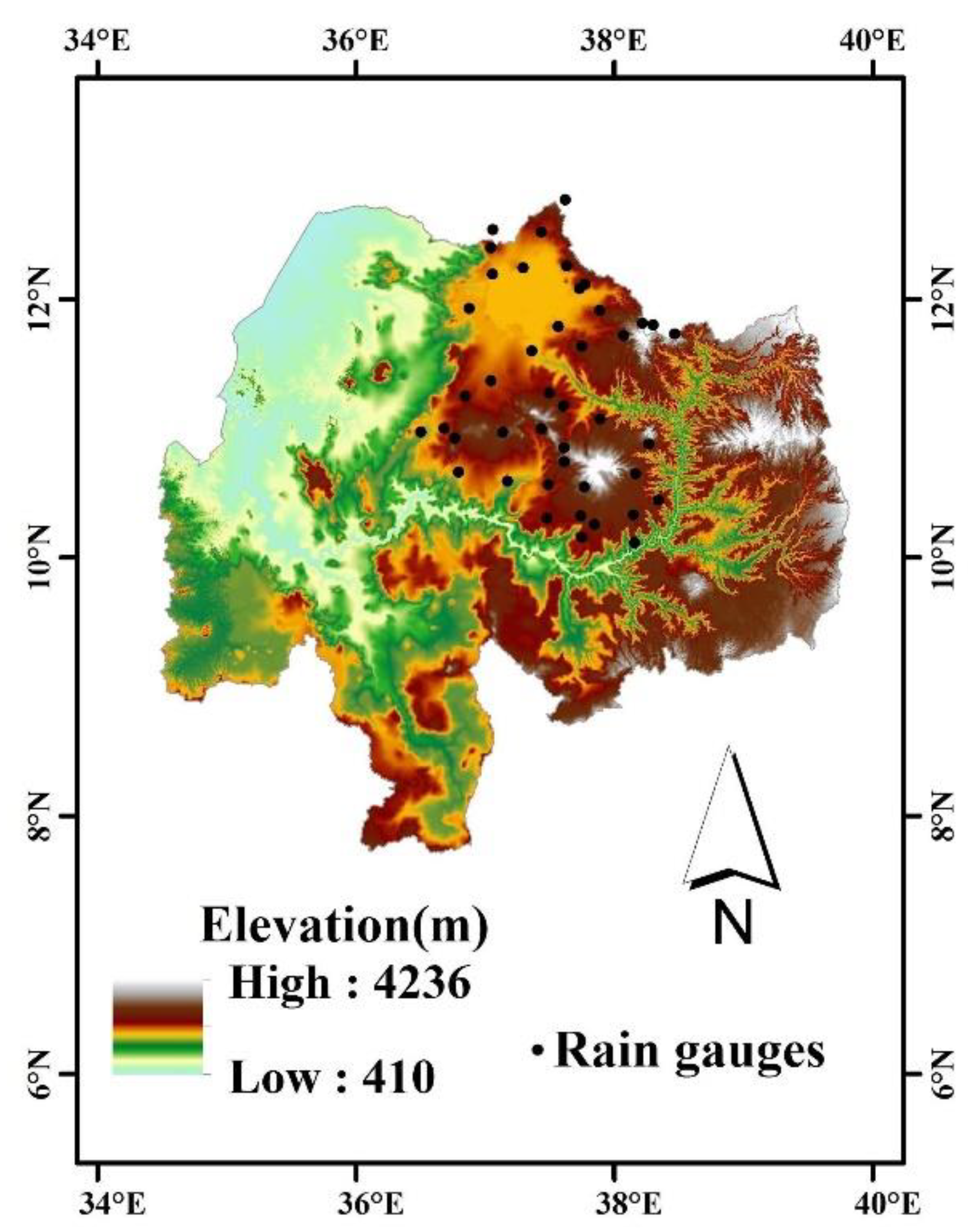
In this research, one complex terrain region, the Upper Blue Nile River basin [3], was selected as our study area. Data were collected from 70 rain gauges between 2000 and 2012. Rain gauges within the same 0.25 degree grids were averaged, and as a result we had 43 grids over the Blue Nile and its corresponding averaged rain gauge values (detail in [3]). Almost the entirety of the rainfall occurs between June and September [3]. The reference dataset was obtained from the above ground-based network, which was mapped at a 0.25 degree grid resolution (interpolation to 0.25 degree grid cells). For our study, five gauge-adjusted quasi-global precipitation products were used: CMORPH, PERSIANN, TMPA or 3B42(V7), GSMaP (V6), and reanalysis (Table 1). Another input feature used in this study was elevation, which ranged between 1615m and 3125m. The positions of rain gauge measurement are shown in Figure 1. The elevation data were collected from the Shuttle Radar Topography Mission (SRTM) dataset. This dataset was obtained using 1° digital elevation model (DEM) tiles from the US Geological Survey and interpolated to a 0.25° grid resolution to match the resolution of the precipitation products. CMORPH, developed by the National Oceanic and Atmospheric Administration (NOAA), calculates precipitation estimates using passive microwave (PMW) observations from low-orbiter satellites, whose features are propagated by geostationary satellite infrared (IR) data. PERSIANN uses neural networks to conduct precipitation estimates based on infrared satellite imagery and ground-surface information. Tropical multi-satellite precipitation analysis (TMPA) estimates precipitation using data from a wide variety of satellite sensors. It is gauge adjusted data that merges IR and PMW precipitation products from the National Aeronautics and Space Administration (NASA). Estimates are provided in both near real time and post real time. GSMaP from the Earth Observation Research Center (EORC) of the Japan Aerospace Exploration Agency (JAXA) uses IR estimates GSMaP-MVK and gauge-adjustment GSMaP (V6). Finally, the reanalysis data were based on the original ERA-Interim data used in ERA-Interim/Land after rescaling based on the Global Precipitation Climatology Center (GPCC) dataset. The dataset used in this study was downscaled using the Climate Hazards Group’s Precipitation Climatology (CHPclim) and bias correction was carried out. The details of these datasets can be found in Ehsan et al. [3].
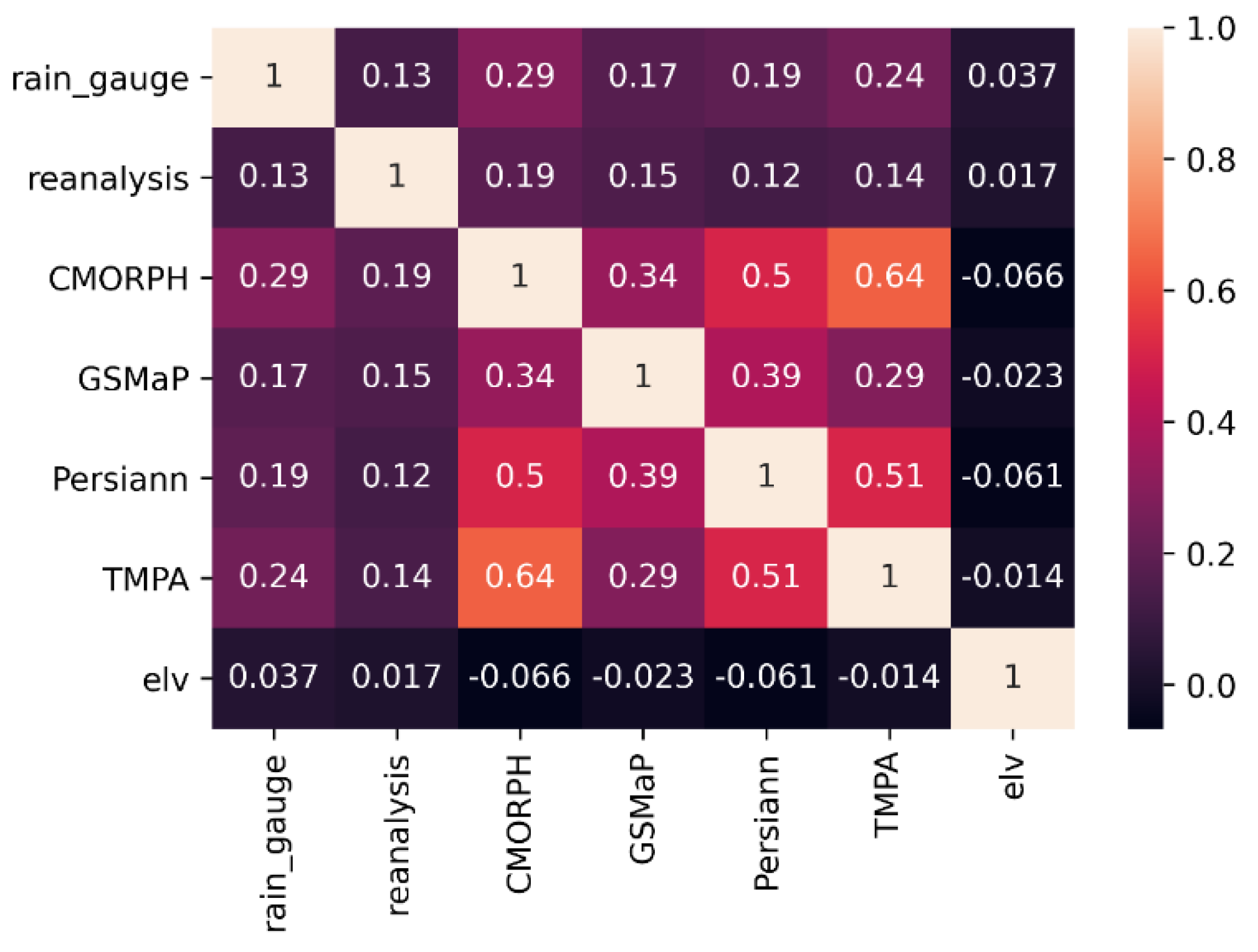
In our study, 53,098 samples of rainfalls were collected, but only the cases where the measured rainfall value was greater than zero were used. The median rainfall was 8.6 mm/day for the rain gauges, with a standard deviation of 9.92 mm/day. Medians and standard deviations for the different models are given in Table 2. The reanalysis data had the closest median and standard deviation (6.94 and 7.91 mm/day, respectively) compared to the rain gauge measurements (8.6, 9.92 mm/day respectively). GSMaP had the lowest median value (2.54 mm/day). Another parameter was the elevation at which the precipitation was measured. The correlation matrix using the Pearson correlation coefficients (Equation (1)) between variables with respect to rain gauge is shown in Figure 2. CMORPH showed a higher correlation (0.29), followed by TMPA (0.24). Elevation had the lowest correlation (0.037).
where r is the correlation coefficient, is the mean of the x values, and is the mean of y values.
3. Methodology
The workflow is shown in Figure 3. In our study, elevation and five precipitation products (‘Reanalysis’, ‘CMORPH’, ‘GSMaP’, ‘PERSIANN’, ‘TMPA’) were used as input features/predictor variables. The input data were normalized using min-max scaling (Equation (2), the resultant data are scaled between 0 and 1). This ensured that every feature had equal significance during training.
where Xnorm is the normalized value after min-max scaling. Xmin and Xmax are the minimum and maximum values of a feature, respectively.
The data were randomly split into train, validation, and test sets. While 70% of the data were used for training algorithms, 10% were used for the optimizing algorithm (Random Forest, Decision Tree, Gradient Boost, Neural Network) parameters (validation), and 20% of the data were used for testing the performance of the algorithms. Each algorithm was considered independently, and the fitting parameters were derived to minimize the loss function: mean square error (MSE). Four regression algorithms were tested.
3.1. Decision Tree Regressor (DT)
This decision tree regressor is a supervised algorithm that predicts outcomes based on decision rules created from prior data. The attributes of the observation are compared with those of the decision tree [28]. Comparison starts from the ‘root’ of the tree, which branches into nodes. Each node in the tree represents a feature and branches into sub-nodes based on the value of that feature. The outcomes are taken from the terminal node or ‘leaf’. In order to develop a model that could accurately predict the output variable without overfitting, decision trees with different maximum depths were fitted to training data and tested on validation data. It was found that a depth of 5 had the lowest mean square error (90.89 mm2/day2) on the validation dataset (Figure 4a). Details about the other parameters used in the algorithm can be found in Table 3.
3.2. Random Forest Regressor (RF)
Random Forest is an ensemble algorithm that uses predictions from a large number of decision trees (weak learners) to obtain a more robust prediction (strong learner) [29]. In RF, a number of decision trees are created from a subset of training data, which are sampled with replacement. Each decision tree also uses a subset of features chosen randomly. This makes the trees less correlated and results in a better performance. The predictions from the decision trees are then averaged to create the final prediction. The RF regressor in our study was optimized by fitting the training data with different numbers of trees and comparing their performance on the validation data. We found that 120 trees perform best, with an MSE of 91.07 mm2/day2 (Figure 4b). Details about the other parameters used in the algorithm can be found in Table 3.
3.3. Gradient Boosting Regressor (GB)
Gradient boosting regressor is also an ensemble method that sequentially combines decision trees [30]. Each tree attempts to minimize the errors of the previous tree. The final prediction aggregates the results from each tree. Similar to RF, the GB regressor was optimized by finding the number of trees (250) that would provide the best performance on the validation dataset (85.62 mm2/day2) (Figure 4c). Details about the other parameters used in the algorithm can be found in Table 3.
3.4. Neural Network (NN)
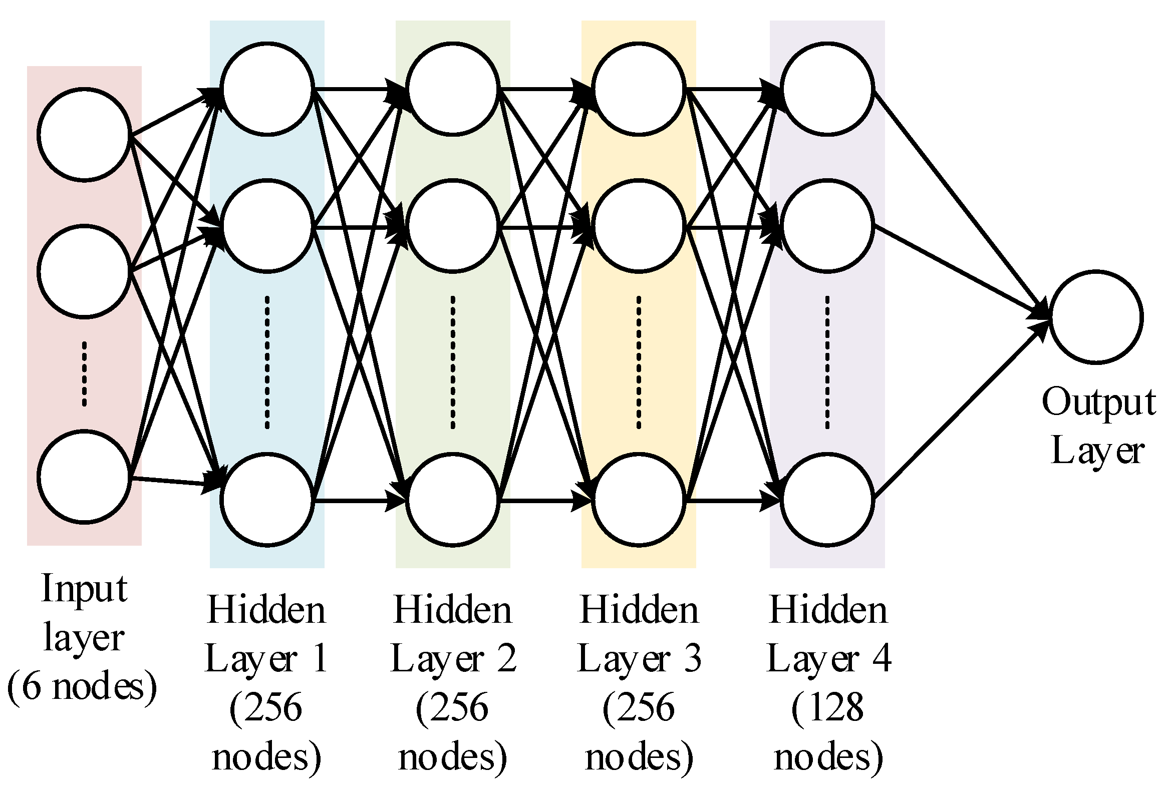
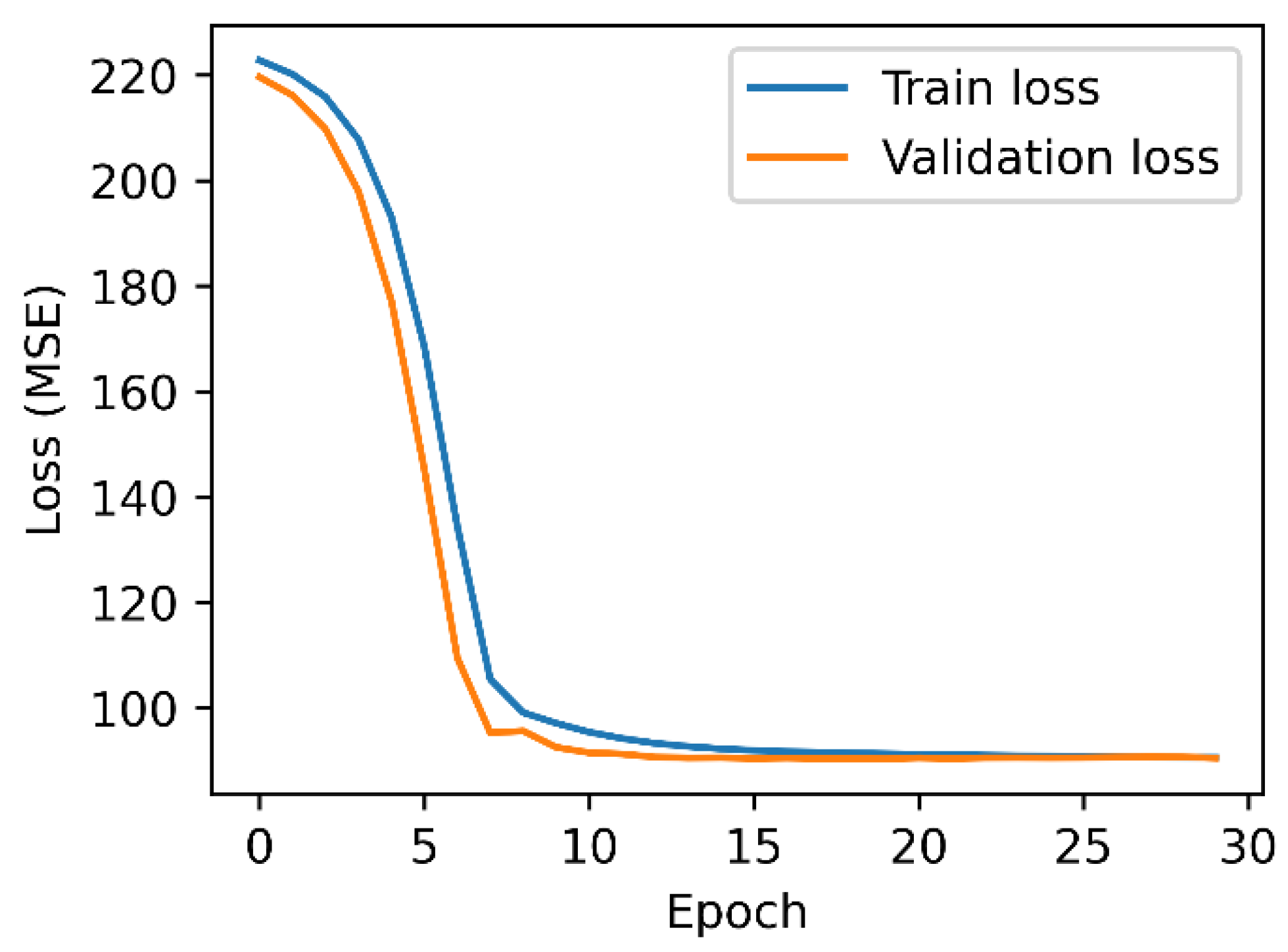
Neural networks are machine learning algorithms comprised of an input layer, one or more hidden layers, and an output layer [31]. Each layer has multiple nodes, with each node generally connected to the input features or outputs from an earlier layer. The output of each node is the weighted sum of inputs to that node. The sum is then fed to an activation function. We used a fully connected NN (every node in a layer is connected to every node in the following layer) with four hidden layers (Figure 5). The input layer consisted of the five input models (CMORPH, PERSIANN, TMPA, GSMaP, and reanalysis) and elevation. The hidden layers contained 256, 256, 256, and 128 nodes, respectively, with rectified linear unit (relu) as their activation function. The output layer predicting precipitation had one node without any activation function. A batch size of 3000 was used. Early stopping was used to prevent overfitting to the training data. The loss versus epoch plots for the training and validation datasets are shown in Figure 6.
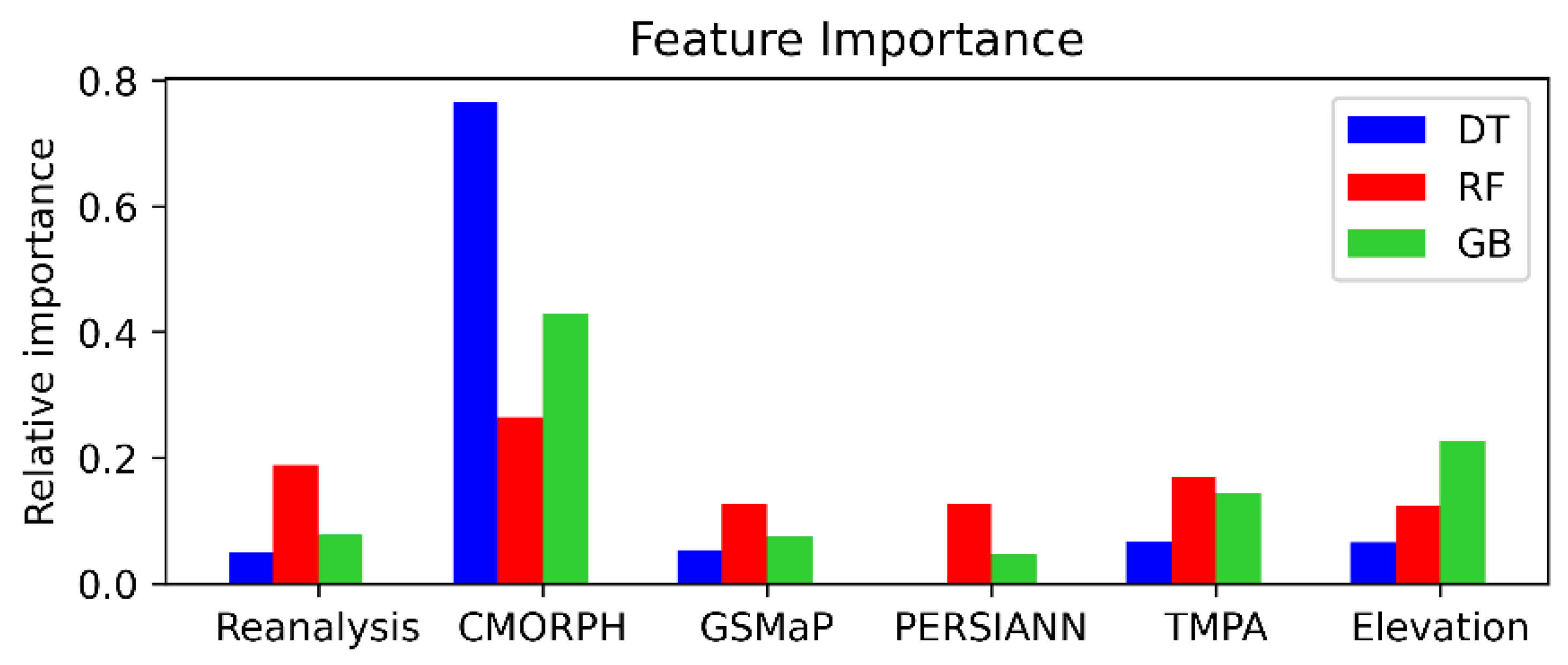
The importance (scale of 0 to 1) of different features for all machine learning algorithms apart from NN are shown in Figure 7. Feature importance is a feature’s contribution to node impurity. CMORPH is most important feature for all algorithms but its weight changes for different algorithms. For examples, it has a relative importance of 0.76 for decision trees but 0.27 for Random Forest. PERSIANN appears to be the feature with the lowest importance overall. This is probably caused by GSMap and PERSIANN reporting zero precipitation for at least up to 25th percentile.
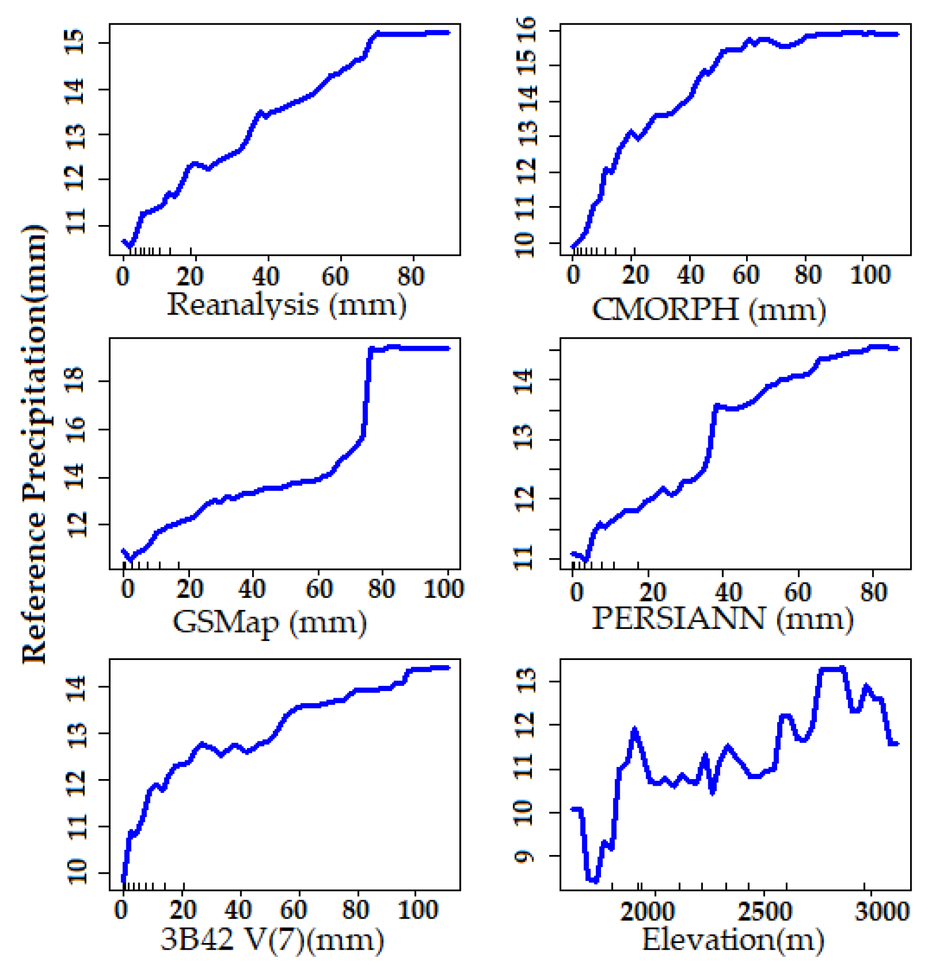
To further demonstrate potential insights into the influence of individual variables on the response variable, a Partial Dependence Plot (PDP) was created for the study area (Figure 8). PDP presents the impact of each variable on the output variable while other variables remain constant [30]. The PDP plot in our study shows the response variable (reference precipitation) responding to all the inputs used in this study. This suggests that the variables selected in our study have a considerable impact on the precipitation prediction, justifying our choice to include them.
4. Performance Evaluation Error Metrics
To compare the performance of algorithms on the test dataset, we decided on the following series of metrics.
4.1. Root Mean Square Error (RMSE) and Normalized Centered Root Mean Square Error (NCRMSE)
Root mean square error is the square root of the mean of sum-squared error terms. The lower the value of RMSE is, the better the model is.
where and are true and predicted values, respectively. N is the population.
Normalized centered root mean square error (NCRMSE) is a statistical metric used to measure random error [32]. The values of NCRMSE vary from zero to positive infinity. The lower the value, the better the performance will be—i.e., there will be lower random error.
4.2. Mean Absolute Error (MAE)
Mean absolute error is the average of absolute values of errors. The lower the value of MAE is, the more accurate it will be.
4.3. Mean Relative Difference (MRD)
Mean relative difference refers to the mean of the relative percentage error, which is given by:
MRD can describe both the magnitude and the direction of the error; positive MRD indicates overestimation, while negative MRD indicates underestimation. A value of zero equates to perfect prediction.
4.4. Bias Ratio (BR)
Bias ratio is the mean of the ratio of the predicted value to the actual value. The bias ratio of a pure unbiased distribution will be 1.
There are two types of errors associated with the precipitation prediction: random error and systematic error. Random errors average out to zero over significant amounts of observation. However, systematic error leads to a consistent deviation from the actual value. NCRMSE quantifies random errors, while MAE, MRD, and BR quantify systematic errors.
5. Results and Discussion
A comparison of the different input models and AI algorithms is shown in Figure 9. For lower than the 25th percentile, GSMaP and CMORPH perform best in terms of RMSE and NCRMSE, respectively. The PERSIAN model performs best in all other metrics (MAE, MRD, and BR). The random error indicated by NCRMSE is reduced by 60% using NN. For all other metrics, GB performs best among the ML algorithms, but falls short of the performance of the input models. For the percentile range between 25th and 50th, the PERSIANN model performed best among the input models in terms of RMSE, MRD, and BR. Reanalysis performed best in NCRMSE and MAE. The ML algorithms performed better than the input models in terms of RMSE (26.1%, NN), NCRMSE (57.5%, GB), and MAE (3.8% GB), although it suffered in terms of MRD and BR. For the 50th to 75th percentile range, the NN model outperformed all the input models, as well as other ML algorithms in all metrics, with 57.6%, 56.4%, 58.2%, 119.6%, and 21% improvements in RMSE, NCRMSE, MAE, MRD, and BR, respectively. For percentiles larger than the 75th, RF performed best among the machine learning models, with 21.9%, 26.33%, 27.2%, 13.9%, and 10.6% improvements over the best input models in terms of RMSE, NCRMSE, MAE, MRD, and BR, respectively. The metric comparison is summarized in Table 4.
In terms of RMSE, the ML algorithms performed worse (<25th percentile, 13% worse) or better (>25th percentile, ≥21% better) than the input models (Figure 9a). Since RMSE puts more weight on larger errors, this indicates that the magnitude of the errors made by ML algorithms decrease as the precipitation value increases. Throughout the entire test set, the ML algorithms had lower random error compared to the input models, as indicated by the NCRMSE plot (Figure 9b). The ML algorithms showed more than 55% improvement over the input models up to the 75th percentile, and 26% improvement beyond that. The mean absolute error plot estimating the average errors shows that ML algorithms performed better than the input models beyond the 25th percentile. Once possible reason behind this may be that the median of the train set is higher than the test set. From the polarity of MRD, we can comment that the ML algorithms overestimate in the 0–75th percentile range and underestimate in the range beyond (Figure 9d). This is because the input models overall show a similar behavior as well. From the bias ratio plot, we observe that the ML algorithms suffer from high bias errors. However, beyond 50th percentile the ML algorithms perform better than the input models (Figure 9e).
Overall, ML algorithms greatly reduced random errors in all percentiles and systematic errors in >50th percentile. They performed best in the 50–75th percentile range and worst in the range below the 25th percentile. The 50-75th percentile is crucial for predicting the growth of vegetation. NN performs best in this range. Even though the input models suffer from high error (RMSE and MAE) in the range above the 75th percentile, we observed improvements in all metrics in this range when using machine learning algorithms. Accurate prediction in this range is important, as it can prevent losses due to flooding caused by excessive rainfall. RF performs best in this range.
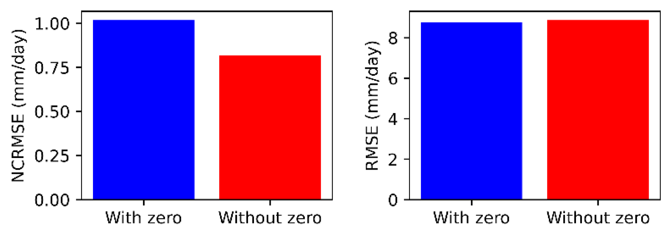
In our analysis so far, we have only considered cases where the measured precipitation was greater than zero. In order to check the robustness of our model, we checked the performance of one of the ML algorithms. GB, for two different datasets: the June-September period of 2000-2012 both ‘with’ and ‘without’ zero precipitation cases. Where zero precipitation cases were included, this constituted ~22% of the dataset. The GB algorithm was trained on 80% of the data and tested on 20% of the data. The resulting NCRMSE and RMSE values are shown in Figure 10. We observed a 19% increase in NCRMSE with the inclusion of zero precipitation, whereas the RMSE reduced by 1.24%. This indicates that zero precipitation cases, if moderate in number, can be handled by ML algorithms. Of course, there will be high bias towards zero for regions or time periods dominated by zero precipitation, resulting in the erroneous prediction of precipitation at higher percentiles.
Overall, for the calibration of the precipitation forecasting model, the most important factors are the AI algorithms, predictors, and accurate precipitation data for constructing a predictor–precipitation relationship. Moreover, AI techniques considered elevation as a control parameter, which helped to decrease the systematic and random error noticeably in the study regions where complex terrain is available. Collective evidence from the recent studies [3,7] and the regional precipitation evaluation study herein shows that hydrological understanding paired with multisource hydrometeorological data merging is necessary for reliable precipitation forecasting over complex terrain areas.
6. Conclusions
This study investigated the use of multisource satellite/reanalysis data for advancing the application of operational water resources. This study also presented a comprehensive evaluation of ML methods and a comparison of reanalysis and satellite-derived estimates of precipitation in the diverse climate and terrain region of the Upper Blue Nile Basin. Understanding complex hydrological processes in conjunction with big data is a prerequisite for predicting water resources phenomena. Although ground-based measurement is the best way to examine the application of water resources, it is impossible to measure all the meteorological information at the required spatio-temporal scale. We used precipitation predictions from five different models and the attribute elevation of the gauge as inputs for four different machine learning algorithms. Elevation showed little correlation with precipitation but was an important feature in making predictions. The performance of the ML algorithms was compared with that of the input models on different metrics, and the ML models improved the predictions in most of the cases, especially in cases above the 25th percentile. The machine learning algorithms tested in this study showed similar improvements in all metrics, with different algorithms showing slightly better performance in each of the four percentile ranges. The ML models also outperformed the input models in the 75 to 100th percentile range. This is crucial, as this range often indicates the flooding of the area. Timely and accurate prediction will alert authorities to take necessary steps to minimize loss if such an event occurs. We found the training time of decision trees to be the shortest, followed by gradient boosting and random forest. Neural networks took the longest time to train. The training time of neural networks can be shortened by using a simpler network, possibly at the cost of accuracy. The neural network was also the most resource intensive. Thus, depending on the resources and degree of precision, different models can be chosen without sacrificing much accuracy, as all the ML models perform better than the input models. In future studies, the observation capability of a single satellite/reanalysis data set could be enriched by utilizing multiple techniques to provide a proof-of-concept for mainstreaming the application of multisource observation-based water management in data-limited regions.
Author Contributions
Conceptualization, M.A.E.B.; methodology, R.S.K.; Software, R.S.K.; validation, R.S.K.; formal analysis M.A.E.B. and R.S.K.; data curation, M.A.E.B.; writing—original draft preparation, M.A.E.B. and R.S.K.; writing—review and editing, M.A.E.B. and R.S.K. All authors have read and agreed to the published version of the manuscript.
Funding
This research received no external funding.
Institutional Review Board Statement
Not applicable.
Informed Consent Statement
Not applicable.
Data Availability Statement
Data available upon request.
Conflicts of Interest
The authors declare no conflict of interest.
References
- Liu, Z. Comparison of versions 6 and 7 3-hourly TRMM multi-satellite precipitation analysis (TMPA) research products. Atmos. Res. 2015, 163, 91–101. [Google Scholar] [CrossRef] [Green Version]
- Mei, Y.; Anagnostou, E.N.; Nikolopoulos, E.I.; Borga, M. Error analysis of satellite precipitation products in mountainous basins. J. Hydrometeorol. 2014, 15, 1778–1793. [Google Scholar] [CrossRef]
- Ehsan Bhuiyan, M.A.; Nikolopoulos, E.I.; Anagnostou, E.N. Machine learning–based blending of satellite and reanalysis precipitation datasets: A multiregional tropical complex terrain evaluation. J. Hydrometeorol. 2019, 20, 2147–2161. [Google Scholar] [CrossRef]
- Derin, Y.; Anagnostou, E.; Berne, A.; Borgo, M.; Boudevillain, B.; Buytaert, W.; Chang, C.-H.; Delrieu, G.; Hong, Y.; Hsu, Y.C.; et al. Multiregional satellite precipitation products evaluation over complex terrain. J. Hydrometeorol. 2016, 17, 1817–1836. [Google Scholar] [CrossRef]
- Grecu, M.; Tian, L.; Olson, W.S.; Tanelli, S. A robust dual-frequency radar profiling algorithm. J. Appl. Meteorol. Climatol. 2011, 50, 1543–1557. [Google Scholar] [CrossRef]
- Huffman, G.J.; Bolvin, D.T.; Braithwaite, D.; Hsu, K.; Joyce, R.; Kidd, C.; Nelkin, E.J.; Xie, P. NASA Global Precipitation Measurement (GPM) Integrated Multi-Satellite Retrievals for GPM (IMERG); Algorithm Theoretical Basis Document Version 06; National Aeronautics and Space Administration: Greenbelt, MD, USA, 2015; Volume 4, p. 26.
- Derin, Y.; Bhuiyan, M.A.E.; Anagnostou, E.; Kalogiros, J.; Anagnostou, M.N. Modeling Level 2 Passive Microwave Precipitation Retrieval Error Over Complex Terrain Using a Nonparametric Statistical Technique. IEEE Trans. Geosci. Remote Sens. 2020, 1–12. [Google Scholar] [CrossRef]
- Weedon, G.P.; Balsamo, G.; Bellouin, N.; Gomes, S.; Best, M.J.; Viterbo, P. The WFDEI meteorological forcing data set: WATCH Forcing Data methodology applied to ERA-Interim reanalysis data. Water Resour. Res. 2014, 50, 7505–7514. [Google Scholar] [CrossRef] [Green Version]
- Rodell, M.; Houser, P.R.; Jambor, U.; Gottschalck, J.; Mitcchell, K.; Meng, C.-J.; Arsenault, K.; Cosgrove, B.; Radakovich, J.; Bosilovich, M.; et al. The global land data assimilation system. Bull. Am. Meteorol. Soc. 2004, 85, 381–394. [Google Scholar] [CrossRef] [Green Version]
- Seyyedi, H.; Anagnostou, E.N.; Beighley, E.; McCollum, J. Hydrologic evaluation of satellite and reanalysis precipitation datasets over a mid-latitude basin. Atmos. Res. 2015, 164, 37–48. [Google Scholar] [CrossRef]
- Dee, D.P.; Uppala, S.M.; Simmons, A.J.; Berrisford, P.; Poli, P.; Kobayashi, S.; Andrae, U.; Balmaseda, M.A.; Balsamo, G.; Bauer, P.; et al. The ERA-Interim reanalysis: Configuration and performance of the data assimilation system. Q. J. R. Meteorol. Soc. 2011, 137, 553–597. [Google Scholar] [CrossRef]
- Shige, S.; Kida, S.; Ashiwake, H.; Kubota, T.; Aonashi, K. Improvement of TMI rain retrievals in mountainous areas. J. Appl. Meteorol. Climatol. 2013, 52, 242–254. [Google Scholar] [CrossRef] [Green Version]
- Hou, A.Y.; Kakar, R.K.; Neeck, S.; Azarbarzin, A.A.; Kummerow, C.D.; Kojima, M.; Oki, R.; Nakumura, K.; Iguchi, T. The global precipitation measurement mission. Bull. Am. Meteorol. Soc. 2014, 95, 701–722. [Google Scholar] [CrossRef]
- Bhuiyan, M.A.E.; Anagnostou, E.N.; Kirstetter, P.E. A nonparametric statistical technique for modeling overland TMI (2A12) rainfall retrieval error. IEEE Geosci. Remote Sens. Lett. 2017, 14, 1898–1902. [Google Scholar] [CrossRef]
- Dinku, T. Challenges with availability and quality of climate data in Africa. In Extreme Hydrology and Climate Variability; Elsevier: Amsterdam, The Netherlands, 2019; pp. 71–80. [Google Scholar]
- Huffman, G.J.; Bolvin, D.T.; Nelkin, E.J.; Wolff, D.B.; Adler, R.F.; Gu, G.; Hong, Y.; Bowman, K.P.; Stocker, E.F. The TRMM Multisatellite Precipitation Analysis (TMPA): Quasi-global, multiyear, combined-sensor precipitation estimates at fine scales. J. Hydrometeorol. 2007, 8, 38–55. [Google Scholar] [CrossRef]
- Joyce, R.J.; Janowiak, J.E.; Arkin, P.A.; Xie, P. CMORPH: A method that produces global precipitation estimates from passive microwave and infrared data at high spatial and temporal resolution. J. Hydrometeorol. 2004, 5, 487–503. [Google Scholar] [CrossRef]
- Ashouri, H.; Hsu, K.-L.; Sorooshian, S.; Braithwaite, D.K.; Knapp, K.R.; Cecil, L.D.; Nelson, B.R.; Prat, O.P. PERSIANN-CDR: Daily precipitation climate data record from multisatellite observations for hydrological and climate studies. Bull. Am. Meteorol. Soc. 2015, 96, 69–83. [Google Scholar] [CrossRef] [Green Version]
- Yamamoto, M.K.; Shige, S.; Yu, C.K.; Cheng, L.-W. Further improvement of the heavy orographic rainfall retrievals in the GSMaP algorithm for microwave radiometers. J. Appl. Meteorol. Climatol. 2017, 56, 2607–2619. [Google Scholar] [CrossRef]
- Bhuiyan, M.A.E.; Yang, F.; Biswas, N.K.; Rahat, S.H.; Neelam, T.J. Machine learning-based error modeling to improve GPM IMERG precipitation product over the brahmaputra river basin. Forecasting 2020, 2, 248–266. [Google Scholar] [CrossRef]
- Bhuiyan, M.A.E.; Nikolopoulos, E.I.; Anagnostou, E.N.; Quintana-Seguí, P.; Barella-Ortiz, A. A nonparametric statistical technique for combining global precipitation datasets: Development and hydrological evaluation over the Iberian Peninsula. Hydrol. Earth Syst. Sci. 2018, 22, 1371–1389. [Google Scholar] [CrossRef] [Green Version]
- Yin, J.; Guo, S.; Gu, L.; Zeng, Z.; Liu, D.; Chen, J.; Shen, Y.; Xu, C.-Y. Blending multi-satellite, atmospheric reanalysis and gauge precipitation products to facilitate hydrological modelling. J. Hydrol. 2021, 593, 125878. [Google Scholar] [CrossRef]
- Chiang, Y.-M.; Hao, R.; Quan, S.; Xu, Y.; Gu, Z. Precipitation assimilation from gauge and satellite products by a Bayesian method with Gamma distribution. Int. J. Remote Sens. 2021, 42, 1017–1034. [Google Scholar] [CrossRef]
- Worqlul, A.W.; Maathuis, B.; Adem, A.A.; Demissie, S.S.; Langan, S.; Steenhuis, T.S. Comparison of rainfall estimations by TRMM 3B42, MPEG and CFSR with ground-observed data for the Lake Tana basin in Ethiopia. Hydrol. Earth Syst. Sci. 2014, 18, 4871–4881. [Google Scholar] [CrossRef] [Green Version]
- Romilly, T.G.; Gebremichael, M. Evaluation of satellite rainfall estimates over Ethiopian river basins. Hydrol. Earth Syst. Sci. 2011, 15, 1505–1514. [Google Scholar] [CrossRef] [Green Version]
- Nicholson, S.E.; Klotter, D.A. Assessing the Reliability of Satellite and Reanalysis Estimates of Rainfall in Equatorial Africa. Remote Sens. 2021, 13, 3609. [Google Scholar] [CrossRef]
- Hirpa, F.A.; Gebremichael, M.; Hopson, T. Evaluation of high-resolution satellite precipitation products over very complex terrain in Ethiopia. J. Appl. Meteorol. Climatol. 2010, 49, 1044–1051. [Google Scholar] [CrossRef]
- Breiman, L.; Friedman, J.; Stone, C.J.; Olshen, R.A. Classification and Regression Trees; CRC Press: Boca Raton, FL, USA, 1984. [Google Scholar]
- Breiman, L. Random forests. Mach. Learn. 2001, 45, 5–32. [Google Scholar] [CrossRef] [Green Version]
- Friedman, J.H. Greedy function approximation: A gradient boosting machine. Ann. Stat. 2001, 29, 1189–1232. [Google Scholar] [CrossRef]
- Barnard, E.; Cole, R.A. A Neural-Net Training Program Based on Conjugate-Gradient Optimization; Oregon Graduate Center: Beaverton, OR, USA, 1989. [Google Scholar]
- Bhuiyan, M.A.E.; Nikolopoulos, E.I.; Anagnostou, E.N.; Polcher, J.; Albergel, C.; Dutra, E.; Fink, G.; la Torre, A.M.; Munier, S. Assessment of precipitation error propagation in multi-model global water resource reanalysis. Hydrol. Earth Syst. Sci. 2019, 23, 1973–1994. [Google Scholar] [CrossRef] [Green Version]
Figure 1.
Map of the elevation of the Upper Blue Nile Region (reprinted with permission from [3]). Black dots indicate the locations of rain gauge measurement.
Figure 1.
Map of the elevation of the Upper Blue Nile Region (reprinted with permission from [3]). Black dots indicate the locations of rain gauge measurement.

Figure 2.
Correlation matrix. A positive/negative (with maximum of +1/−1) value indicates a positive/negative relationship (if one value increases, the other increases/decreases) between variables. A value of 0 indicates no relationship.
Figure 2.
Correlation matrix. A positive/negative (with maximum of +1/−1) value indicates a positive/negative relationship (if one value increases, the other increases/decreases) between variables. A value of 0 indicates no relationship.

Figure 3.
Schematic representation of the prediction process for this study.

Figure 4.
Optimization of the decision tree regressor (a), random forest regressor (b), gradient boosting regressor (c) algorithms. Unit for mean square error is (mm/day)2.
Figure 4.
Optimization of the decision tree regressor (a), random forest regressor (b), gradient boosting regressor (c) algorithms. Unit for mean square error is (mm/day)2.

Figure 5.
Schematics of the neural network used in this study.

Figure 6.
Neural network training and validation loss plots. Training was stopped at epoch 34 to prevent overfitting to the training data.
Figure 6.
Neural network training and validation loss plots. Training was stopped at epoch 34 to prevent overfitting to the training data.

Figure 7.
Relative importance of the input features for different algorithms.

Figure 8.
Partial Dependence Plot (PDP) of the features used in this study.

Figure 9.
Percentile-based comparison of RMSE (a), NCRMSE (b), MAE (c), MRD (d), and BR (e) between input models and different machine learning algorithms on the test dataset. Total number of samples in test set was 10,620; thus, each of the four percentile ranges contain 2655 samples. The 0th, 25th, 50th, 75th, and 100th percentile values are 0.03, 3.8, 8.5, 15.2, and 124 mm/day, respectively. The preferred value for BR (=1) is indicated by a black dashed line.

Figure 10.
NCRMSE and RMSE for test datasets with (blue) and without (red) zero precipitation included.
Figure 10.
NCRMSE and RMSE for test datasets with (blue) and without (red) zero precipitation included.


Table 1.
Spatiotemporal resolution of different precipitation products used in this study.
| Precipitation Product | Original Spatiotemporal Resolution |
|---|---|
| TMPA | 0.25 degree, daily |
| CMORPH | |
| PERSIANN | |
| ERA-Interim | |
| GSMap | 0.1 degree daily |
Table 2.
Percentiles and standard deviations of rainfall prediction from models as well as the measured rainfall (Target). All units are mm/day.
Table 2.
Percentiles and standard deviations of rainfall prediction from models as well as the measured rainfall (Target). All units are mm/day.
| Reanalysis | CMORPH | GSMaP | PERSIANN | TMPA | Rain Gauge | |
|---|---|---|---|---|---|---|
| Min (0%) | 0 | 0 | 0 | 0 | 0 | 0.02 |
| 25% | 4.09 | 2.25 | 0 | 0 | 1.25 | 3.8 |
| Median (50%) | 6.94 | 6.09 | 2.54 | 2.97 | 5.15 | 8.6 |
| 75% | 11.47 | 12.60 | 9.26 | 9.06 | 11.90 | 15.4 |
| Max (100%) | 89.26 | 112.05 | 100.00 | 86.61 | 110.91 | 166 |
| Standard Deviation | 7.91 | 9.71 | 8.63 | 8.74 | 9.85 | 9.92 |
Table 3.
Additional parameters for the decision tree, random forest, and gradient boosting regressors used in this study.
Table 3.
Additional parameters for the decision tree, random forest, and gradient boosting regressors used in this study.
| Parameter | Description | DT | RF | GB |
|---|---|---|---|---|
| Criterion | Function to measure the quality of a split | Mean Square Error (MSE) | MSE | MSE |
| Number of estimators | Number of trees in the forest | N/A | Figure 3b | Figure 3c |
| Splitter | Strategy to choose the split at each node | Best | N/A | N/A |
| Max Depth | Maximum depth of the tree | Figure 3a | until all leaves contain less than minimum samples for splitting (2) | 3 |
| Min samples at leaf node | Minimum number of samples required to be at a leaf node | 1 | 1 | 1 |
| Bootstrap | Using bootstrap samples to build the tree | N/A | True | N/A |
Table 4.
Best input and ML model based on different metrics in different percentile ranges. Red indicates a worse performance than the input models and green indicate a better performance.
Table 4.
Best input and ML model based on different metrics in different percentile ranges. Red indicates a worse performance than the input models and green indicate a better performance.
| Percentile(th) | RMSE | NCRMSE | MAE | MRD | BR | |
|---|---|---|---|---|---|---|
| <25 | Best input | GSMaP | CMORPH | PERSIANN | PERSIANN | PERSIANN |
| Best ML Model | GB | NN | GB | GB | GB | |
| Performance (%) | 13.7 | 60.0 | 80.9 | 187.5 | 146.6 | |
| 25-50 | PERSIANN | Reanalysis | Reanalysis | PERSIANN | PERSIANN | |
| NN | NN | GB | GB | GB | ||
| 26.1 | 57.5 | 3.8 | 11,549.7 | 90.2 | ||
| 50-75 | Reanalysis | Reanalysis | Reanalysis | Reanalysis | Reanalysis | |
| NN | NN | NN | NN | NN | ||
| 57.6 | 56.4 | 58.2 | 119.6 | 21.0 | ||
| >75 | CMORPH | Reanalysis | CMORPH | CMORPH | CMORPH | |
| RF | DT | RF | RF | RF | ||
| 21.9 | 26.3 | 27.2 | 13.9 | 10.6 |
Publisher’s Note: MDPI stays neutral with regard to jurisdictional claims in published maps and institutional affiliations. |
© 2021 by the authors. Licensee MDPI, Basel, Switzerland. This article is an open access article distributed under the terms and conditions of the Creative Commons Attribution (CC BY) license (https://creativecommons.org/licenses/by/4.0/).
Share and Cite
MDPI and ACS Style
Khan, R.S.; Bhuiyan, M.A.E. Artificial Intelligence-Based Techniques for Rainfall Estimation Integrating Multisource Precipitation Datasets. Atmosphere 2021, 12, 1239. https://doi.org/10.3390/atmos12101239
AMA Style
Khan RS, Bhuiyan MAE. Artificial Intelligence-Based Techniques for Rainfall Estimation Integrating Multisource Precipitation Datasets. Atmosphere. 2021; 12(10):1239. https://doi.org/10.3390/atmos12101239
Chicago/Turabian StyleKhan, Raihan Sayeed, and Md Abul Ehsan Bhuiyan. 2021. "Artificial Intelligence-Based Techniques for Rainfall Estimation Integrating Multisource Precipitation Datasets" Atmosphere 12, no. 10: 1239. https://doi.org/10.3390/atmos12101239
Note that from the first issue of 2016, this journal uses article numbers instead of page numbers. See further details here.