Experimental Validation of a Mathematical Model to Describe the Drug Cytotoxicity of Leukemic Cells

Abstract

Chlorambucil (Chl), Melphalan (Mel), and Cytarabine (Cyt) are recognized drugs used in the chemotherapy of patients with advanced Chronic Lymphocytic Leukemia (CLL). The optimal treatment schedule and timing of Chl, Mel, and Cyt administration remains unknown and has traditionally been decided empirically and independently of preclinical in vitro efficacy studies. As a first step toward mathematical prediction of in vivo drug efficacy from in vitro cytotoxicity studies, we used murine A20 leukemic cells as a test case of CLL. We first found that logistic growth best described the proliferation of the cells in vitro. Then, we tested in vitro the cytotoxic efficacy of Chl, Mel, and Cyt against A20 cells. On the basis of these experimental data, we found the parameters for cancer cell death rates that were dependent on the concentration of the respective drugs and developed a mathematical model involving nonlinear ordinary differential equations. For the proposed mathematical model, three equilibrium states were analyzed using the general method of Lyapunov, with only one equilibrium being stable. We obtained a very good symmetry between the experimental results and numerical simulations of the model. Our novel model can be used as a general tool to study the cytotoxic activity of various drugs with different doses and modes of action by appropriate adjustment of the values for the selected parameters.

1. Introduction

CLL is the most common leukemia in adults and is characterized by the uncontrolled growth of mature B lymphocytes (B cells) [1]. Advances in basic research and therapeutics over the last few years have significantly improved the treatment and clinical outcomes of patients with CLL [2,3,4,5]. Nonetheless, new mathematical models that could aid researchers and clinicians to decide how best to combine traditional and novel agents and to sequence these treatments might result in a reduction in the treatment side effects and the development of drug resistance, which would in turn lead to deep and long-term remissions.

Mathematical modeling of cancer growth has a long history and has been reviewed before [6,7,8,9]. Ordinary Differential Equations (ODE) are used in mathematical models to define the modification of continuous variables and to consider the change over time or space and may vary in complexity from a single equation to multivariable systems. Earlier efforts led to the creation of models with a simplified empirical structure, presented as ODEs, describing the growth of tumor size using exponential or sigmoidal functions [10]. Over the past decade, several mathematical models have described the dynamics of blood cancers under the influence of various drugs and/or immunotherapy [11,12,13,14]. With special regard to CLL, several studies [15,16,17] have modeled the interaction between peripheral blood lymphocytes and CLL cells. These studies produced dynamic systems and identified parameters that describe the growth rate of cancer cells. Kuznetsov et al. [18] was one of the first groups to provide a sensitivity analysis and to describe the observation that cancer cells remain in an apparently dormant state for a prolonged time before entering a rapid growth phase. More recently, Reference [19] used a compartmental model to separate circulating CLL cells from those in lymphoid tissues. This model tracked the production of new CLL cells and showed that the growth rate and death rate of CLL cells are similar. These examples demonstrate that mathematical modeling can have various applications in cancer therapy. However, a major limitation of these quantitative models is that they are not based on real-life experimental data. Furthermore, these models depict the relationship between CLL growth and the immune response to it, but they do not describe or predict the optimal use of drugs for this disease.

Previous studies have explored combining tumor growth kinetics and drug pharmacokinetics with computational machine learning to predict the treatment sequence [20], drug neurotoxicity, and efficacy in drug discovery [21,22]. However, machine learning requires large datasets, and the resulting algorithm is not readily available to the investigator. The model described in our work was based on that used by [23], who employed a system of ODEs to study chemotherapy and immunotherapy in CLL, but we introduced modifications and focused on the effect of chemotherapy on CLL cell growth.

We first grew A20 murine leukemic cells as a surrogate for CLL cells and described their growth rate mathematically. We then tested in vitro the cytotoxicity of three drugs, Chlorambucil (Chl), Melphalan (Mel), and Cytarabine (Cyt), against the cells, using the results to build a dynamic model that incorporates both cancer cell growth and death rates in relation to drug concentration. We then performed model validation and finally a stability analysis. Our results led to the development of a new model that allows the prediction of the optimal drug concentration that will produce the maximum death of cancer cells. Our novel model can be used as a general tool to study the cytotoxic activity of various drugs with different doses and modes of action by appropriate adjustment of the values for the selected parameters.

2. Materials and Methods

2.1. Cells and Reagents

A20 murine leukemic cells (obtained from the ATCC, VA, USA) were grown in RPMI 1640 (Thermo Fischer Scientific, Waltham, MA, USA). All media were supplemented with 10% Fetal Bovine Serum (FBS) (Thermo Fischer), 1% L-glutamine, and 0.33% Pen-Strep solution. Cells were maintained at 37 °C and 5% CO${}_2$. Cell growth was measured with the XTT-based Cell Proliferation Kit (Biological Industries, Bet Haemek, Israel) according to the manufacturer’s instructions.

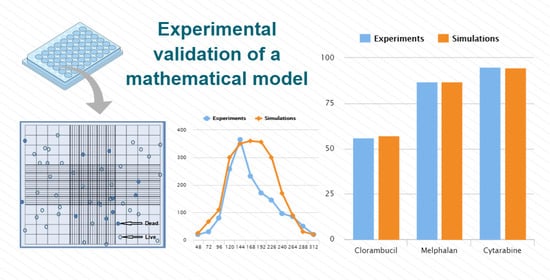
To determine the growth rate, A20 cells were seeded at three concentrations: $5\times {10}^3$; $1\times {10}^4$, and $5\times {10}^4/$mL. An aliquot was taken from the cultures every 12 h from the 48th until the 312th hour for total and viable cell counting. Experiments were repeated three times. The cells were stained using trypan blue, and live and dead cells were counted with a hemocytometer from duplicate samples of the same culture (Figure 1).

2.2. Drug Cytotoxicity Assay

We chose to study the effect of three drugs known to induce cell death by interfering with DNA replication by different mechanisms. Chlorambucil is an alkylating agent that induces cross-links between DNA strands, resulting in interference with DNA replication [24]. Melphalan alkylates guanine, which leads to interstrand and intrastrand DNA adducts, resulting in inhibition of DNA and RNA synthesis and eventual cell death [25]. Cytarabine, also known as arabinosylcytosine (ARA-C), is a pyrimidine analog and competes with cytidine for incorporation into the DNA, leading to cessation of DNA replication and DNA damage response mechanisms [26].

Drug cytotoxicity was determined by culturing A20 cells in macroplate wells (Nunclon) at an initial concentration of $5\times {10}^4$/well for 72 h in culture medium containing either Chl, Mel, or Cyt at concentrations ranging from 0–50 µM. Cell viability was assessed by using the XTT assay, which measures cellular ATP levels. Absorbance in the wells was measured at 450 nm and subtracted from the reference absorbance at 630 nm. Culture medium was used as the background control.

2.3. Validation of the Model

The data from the in vitro experiments and the parameters from

Table 1. Table of parameters based on experimental results related to the model of Equations (3)–(5).

Parameter	Physical Interpretation (Units)	Estimated Value	Reference
t	Time of cell culture (h)	0–312	Experimental data
r	A20 growth rate (h${}^{-1}$)	$0.07$	Experimental data
K	Maximal tumor cell population (cells/mL)	$4\times {10}^6$	Experimental data
${\mu }_A$	Living cells become dead (h${}^{-1}$)	$3.7\times {10}^{-8}$	From simulation
a	Drug dose that produces 50% maximum effect (mL)	$2\times {10}^3$	From [27]
${\mu }_{AC}$	Cytotoxicity rate in the presence of drug (h${}^{-1}$)	see Table A1, Table A2 and Table A3	From simulation
${\mu }_{CA}$	Deactivation rate of drug due to killing of A20 cells (h${}^{-1}$)	${\mu }_{AC}\times 10$	From simulation
${\mu }_C$	Chemical deactivation rate of drug (h${}^{-1}$)	0.462—Chl; 0.347—Mel; 0.231—Cyt	From [28]
d	Dissolution rate of dead A20 cells (h${}^{-1}$)	$0.017$	From simulation

were used to validate our model. In addition, computer simulations were performed using fourth-order adaptive step Runge–Kutta integration, as implemented in the ODE45 subroutine of MATLAB.

3. Results and Discussion

3.1. Cell Growth and Death Dynamics

To determine cell growth and death rates, A20 cells were sampled every 12 h for total and viable cell counts (Figure 2). The natural decrease in cell viability after the maximum peak was due to suboptimal growth conditions resulting from nutrient deprivation, decreased pH, and cell overcrowding, which induces cell death by necrosis and apoptosis [29].

3.2. Drug Cytotoxicity

Cells were cultured for 72 h in fresh medium containing either Chl, Mel, or Cut, and the cellular metabolic status was determined. The results are shown in Figure 3.

As can be seen above (Figure 3), Chl was the least effective of the three drugs, producing only 56% cell growth inhibition at the maximum concentration used in the experiment, 50 $\mathsf{\mu }$M, while Mel induced 92% inhibition at this dose. At the lowest dose of 1.56 $\mathsf{\mu }$M, Chl induced only 7% growth inhibition, while Mel induced 49% inhibition. On the other hand, Cyt maintained a high plateau level of growth inhibition of between 96% and 92% inhibition down to 3.125 $\mathsf{\mu }$M.

These experiments provided the basis for the development of our dynamic model.

3.3. Formulation of the Model

Based on cell counts with a hemocytometer (Figure 1 and Figure 2), A20 cells can be divided into two groups: live cells (transparent circle in Figure 1) and dead cells (blue circle in Figure 1), denoted as A and $A_d$, respectively, in the mathematical model developed by us. Dead cells ($A_d$) are formed because of apoptosis and/or necrosis in culture after the death of living A cells. The death rate of living A cells depends on several conditions in the culture environment: the concentration of essential nutrients in the cells, the supply and uptake of oxygen, and the disposal of waste products such as ammonia and various acidic products [29,30,31]. The total number of living and dead cells cannot exceed a certain capacity (K) in the closed space of the culture. The dynamics of living and dead cells of type A20 in a closed environment is described using differential equations as follows:

$$\begin{array}{cc}\{& \begin{array}{}\mathrm{(1)}& \frac{dA}{dt}=rA(1-\frac{A}{K})-{\mu }_{A}A{A}_d\hfill \mathrm{(2)}& \frac{d{A}_d}{dt}={\mu }_{A}A{A}_d-d{A}_d\hfill \end{array}\end{array}$$

${\displaystyle \frac{dA}{dt}}$ describes the dynamics of living A20 cells. It comprises two terms: one positive, corresponding to the logistic cancer growth characterized by the coefficient, r, which is limited by the maximal tumor cell number, K; one negative term, corresponding to living cells becoming dead at a rate of ${\mu }_A$.

${\displaystyle \frac{d{A}_d}{dt}}$ describes the dynamic of dead A20 cells. It is comprised of two terms: the positive term is the death of A20 cells with a rate coefficient of ${\mu }_A$ due to apoptosis or necrosis and depends on living A20 cells competing for survival (oxygen consumption and nutrition) in an enclosed space; the negative term corresponds to dissolution of dead cells at a rate of d.

We extended the model by adding a new equation that represents the dynamics of chemotherapeutic drugs. Based on previous studies [23] and our experiments in vitro, we formulated an ODE model to mathematically explain the interaction between CLL cells and chemotherapeutic drugs:

$$\begin{array}{cc}\{& \begin{array}{}\mathrm{(3)}& \frac{dA}{dt}=rA(1-\frac{A}{K})-{\mu }_{A}A{A}_d\underset{\underset{\mathrm{t}\mathrm{e}\mathrm{r}\mathrm{m} 1}{︸}}{-\frac{{\mu }_{AC}AC}{a+C}},\hfill \mathrm{(4)}& \frac{d{A}_d}{dt}={\mu }_{A}A{A}_d-d{A}_d\underset{\underset{\mathrm{t}\mathrm{e}\mathrm{r}\mathrm{m} 2}{︸}}{+\frac{{\mu }_{AC}AC}{a+C}},\hfill \mathrm{(5)}& \frac{dC}{dt}={\mu }_{C}C-\frac{{\mu }_{CA}CA}{a+C},\hfill \end{array}\end{array}$$

${\displaystyle \frac{dC}{dt}}$ describes the first-order pharmacokinetics of a drug [32]. The drug was given only once at the beginning of the experiment, i.e., $C\left(0\right)$ is a constant value and depends on the dose of the drug.

${\mu }_C$ is the deactivation rate calculated by formula ${\mu }_C=\frac{ln\left(2\right)}{t_{1/2}}$, where $t_{1/2}$ is the in vitro elimination half-life, about 1.5 h for Chl, 2 h for Mel, and 1–3 h (biphasic) for Cyt (www.drugbank.ca accessed on 17 September 2021).

The terms 1 and 2 of the Equations (3) and (4) represent the log-kill hypothesis [33], with a Michaelis–Menten drug saturation response [34], $a+C$; ${\mu }_{AC}$ is the death rate resulting from the action of the drug on the cancer cells. The parameter ${\mu }_{AC}$ changes depending on the drug dose and on the particular drug. We chose the parameter ${\mu }_{CA}$ to be ten-times more than ${\mu }_{AC}$, assuming that there are 10–100 drug molecules attacking each cancer cell. Ultimately, the parameter ${\mu }_{CA}$ does not play a significant role in the model, since there are many more drug molecules than cancer cells, and it only reflects the amount of available drug molecules. The parameter a represents the drug concentration that produces 50% of the maximum activity of the drug in each cell population [27].

We performed a mathematical analysis of our model by identifying fixed points and their stability. It was found that the system is characterized by three fixed points, one of which is stable asymptotically (Appendix A,

Table A4. Summary of the stability analysis.

Fixed Points	${\mathit{A}}^{*}$	${\mathit{A}}_{\mathit{d}}^{*}$	${\mathit{C}}^{*}$	Stability
$E_0^{*}$	0	0	0	unstable
$E_1^{*}$	${\displaystyle \frac{d}{{\mu }_A}}$	${\displaystyle \frac{r}{{\mu }_A}}-{\displaystyle \frac{rd}{K{\mu }_A^2}}$	0	asymptotically stable
$E_2^{*}$	K	0	0	unstable

).

3.4. Estimation of the Parameters of the Model

In this section, we evaluate the model parameters (Table 1), together with the detailed methods and the literature sources for their evaluation:

• $A\left(0\right)=5\times {10}^4$ (cells/mL)—the initial number of A20 cells;
• $A_d\left(0\right)=2500$ (cells/mL)—the initial number of dead A20 cells (cell cultures commonly consist of at least 5% of dead cells);
• $C\left(0\right)=$ dose ($\mathsf{\mu }$M) $\times 6\times {10}^{14}$ (number of drug molecules/mL)—the dose concentration of Chl, Mel, or Cyt (this number may vary depending on the drug, but not significantly since all these drugs are related to the same type of small molecules).

The number of drug molecules was calculated using the formula:

$${\displaystyle Thenumberofdrugmolecules=\frac{m\times Na}{M}},$$

where:

• m = the mass of drug in kg;
• $Na$ = Avogadro number = $6.022\times {10}^{23}$ (constant);
• M = the molar mass of drug (Chl 304.212 g/mol; Mel 305.2 g/mol; Cyt 243.217 g/mol).

For example, for 50 µM of Chl, i.e., 50 µM = 15.15 µL = 0.00001515 kg, it would be:

$${\displaystyle ThenumberofChlmolecules=\frac{0.00001515\times 6.022\times {10}^{23}}{304.212}}=3\times {10}^{16}=50\times 6\times {10}^{14}.$$

The cell doubling time was calculated using an exponential growth rate:

$$N\left(t\right)=N\left(0\right)e^{rt}$$

or

$${\displaystyle r=\frac{ln\left(N\left(t\right)/N\left(0\right)\right)}{t}},$$

where:

• $N\left(t\right)$ = the number of cells at time t;
• $N\left(0\right)$ = the number of cells at Time 0;
• r = growth rate;
• t = time (usually in hours).

The tumor doubling time is calculated as:

$${\displaystyle \mathrm{TDT}=\frac{ln\left(2\right)}{\mathrm{growth}\mathrm{rate}}}.$$

Thus, according to Figure 2, when $N\left(0\right)=12\times {10}^4$ by the 84th hour, $N\left(t\right)=349\times {10}^4$ by the 132th hour, and $t=132-84=48$, the growth rate of A20 cells would be:

$${\displaystyle r=\frac{ln\left(3490000/120000\right)}{48}}=0.07\left({\mathrm{h}}^{-1}\right),$$

and the cell doubling time would be:

$${\displaystyle \mathrm{TDT}=\frac{ln\left(2\right)}{0.07}=9.9}\left(\mathrm{h}\right).$$

Thus, according to Figure 2 the number of A20 cells double in less than 12 h.

The parameters used in this study are summarized in Table 1.

3.5. Validation of the Cancer Cell Growth Dynamics Model

Figure 4 compares the numerical simulations and the in vitro experimental growth and natural death curves for A20 cells at different starting cell concentrations.

To assess the closeness of the fit between the simulation and experimental curves, the root-mean-squared errors (RMSEs) were calculated using the formula:

$$RMSE=\sqrt{\frac{{\sum }_i^n{(Si{m}_i-Ex{p}_i)}^2}{n}},$$

where $Sim$ is the numerical simulation data (predicted value), $Exp$ is the experimental data (observed value), and n is the number of observations (see Appendix A,

Table A5. Comparison of CLL cell growth dynamics (cells/mL) between experimental data and numerical simulations.

	$5\times {10}^4$		$1\times {10}^4$		$5\times {10}^3$
Time (h)	Exp	Sim	Exp	Sim	Exp	Sim
48	50,000	54,054	10,000	10,070	10,000	5228
60	70,000	122,897	10,000	22,602	10,000	8821
72	100,000	273,025	10,000	50,236	10,000	14,854
84	120,000	577,722	30,000	109,941	20,000	24,948
96	590,000	1,114,930	80,000	234,397	30,000	41,736
108	1,850,000	1,862,730	80,000	477,462	40,000	69,424
120	2,580,000	2,621,770	320,000	900,296	120,000	114,512
132	3,490,000	3,180,420	800,000	1,509,560	130,000	186,545
144	3,650,000	3,498,490	1,190,000	2,184,030	550,000	298,370
156	2,440,000	3,641,320	3,120,000	2,732,350	820,000	464,737
168	2,320,000	3,654,730	3,070,000	3,052,090	1,030,000	697,464
180	2,020,000	3,500,150	2,950,000	3,162,600	1,300,000	996,212
192	1,710,000	3,062,170	2,760,000	3,125,520	1,440,000	1,338,190
204	1,550,000	2,364,930	2,120,000	2,990,300	1,600,000	1,676,040
216	1,450,000	1,672,210	2,020,000	2,785,060	1,770,000	1,951,030
228	1,240,000	1,149,160	1,900,000	2,523,550	1,980,000	2,114,600
240	960,000	779,597	1,540,000	2,212,900	2,160,000	2,141,610
252	870,000	551,455	1,240,000	1,859,650	2,050,000	2,029,460
264	850,000	388,608	1,030,000	1,474,810	1,900,000	1,791,020
276	720,000	276,498	980,000	1,078,450	1,440,000	1,451,290
288	500,000	198,206	750,000	702,772	1,030,000	1,050,550
300	210,000	142,884	520,000	388,800	880,000	648,799
312	50,000	103,435	160,000	171,158	240,000	318,579
RMSE	0.016		0.013		0.008

).

The RMSEs for the initial cell concentrations are: $5\times {10}^4$ cells/mL = 0.016; $1\times {10}^4$ cells/mL = 0.013; $5\times {10}^3$ cells/mL = 0.008. The data showed a strong correlation between the simulation and experimental results for both the time and cell concentration at both the maximum and final data points. The correlation held for all three starting concentrations (all RMSEs were < 0.1), but was most symmetric for the lowest starting concentration ($5\times {10}^3$ cells/mL).

3.6. Validation of the Cancer Cell Drug Cytotoxicity Dynamics Model

By inserting the parameters from Table 1 into Equations (2) and (3), we could numerically simulate the effect of Chl, Mel, or Cyt on A20 cells, as depicted in Figure 5.

After 72 h, the concentration of A20 growth without drug increased to A(72) = 1,646,260. The additional 50 µM of Chl (A) reduced the growth to A(72) = 717,369 cells/mL, which equals 56.4% growth inhibition; 50 µM of Mel induced $92\%$ growth inhibition (B), and 6.25 µM of Cyt induced $94.8\%$ growth inhibition (C). The complete set of calculated data for all drug concentrations is presented in Appendix A (

Table A1. Simulated effect of chlorambucil on A20 growth parameters.

Concentration of Chl (µM)	Parameter ${\mathit{\mu }}_{\mathbf{AC}}$	Number of Cells at 72nd Hour (cells/mL)	Cell Growth Inhibition (%)
0	-	1,646,260	0
50	0.018	717,369	56.4
25	0.0126	913,673	44.5
$12.5$	0.0088	1,089,350	33.8
$6.25$	0.006	1,235,190	25
$3.125$	0.004	1,349,710	18
$1.5625$	0.003	1,435,539	12.8

,

Table A2. Simulated effect of melphalan on A20 growth parameters.

Concentration of Mel (µM)	Parameter ${\mathit{\mu }}_{\mathbf{AC}}$	Number of Cells at 72nd Hour (cells/mL)	Cell Growth Inhibition (%)
0	-	1,646,260	0
50	0.0397	132,518	92
25	0.0278	240,547	85.4
$12.5$	0.0195	388,950	76.4
$6.25$	0.0136	567,233	65.5
$3.125$	0.0095	757,405	54
$1.5625$	0.0067	940,943	42.8

and

Table A3. Simulated effect of cytarabine on A20 growth parameters.

Concentration of Cyt (µM)	Parameter ${\mathit{\mu }}_{\mathbf{AC}}$	Number of Cells at 72nd Hour (cells/mL)	Cell Growth Inhibition (%)
0	-	1,646,260	0
$6.25$	0.046	85,683	94.8
$3.125$	0.0322	168,014	89.8
$1.5625$	0.0225	291,671	82.3
$0.78$	0.0158	452,951	72.5
$0.39$	0.011	637,807	61.3
$0.195$	0.0077	827,114	49.7
$0.098$	0.0054	1,003,650	39
$0.049$	0.0038	1,156,420	29.7
$0.024$	0.0026	1,281,250	22.2
$0.012$	0.0018	1,378,920	16.2
$0.006$	0.0013	1,452,970	11.7

).

We then compared the degree of A20 growth inhibition from the numerical simulation of the model (Equations (3)–(5)) (Figure 5) with the output obtained by the in vitro experiments (Figure 3). The results are shown in Figure 6.

Figure 6 demonstrates that our simulation coincided with the experimental data for the high doses of each drug. For the intermediate doses, there appeared to be a slight deviation between the two sets of data. This deviation was artificial since we tried to maintain consistency in the decrease of the parameter ${\mu }_{AC}$ in accordance with the decrease in the drug dose. This resulted in a discrepancy of 30% for each drug. However, it is important to note that maintaining this consistency is not necessary, and it is possible to juxtapose the experimental and simulation results with absolute accuracy by choosing the appropriate parameter ${\mu }_{AC}$.

The RMSE for each drug was calculated (see Appendix A,

Table A6. Comparison of cell growth inhibition (%) between experimental data and numerical simulations.

Concentration of Drug (µM)	Chlorambucil		Melphalan		Cytarabine
	Exp	Sim	Exp	Sim	Exp	Sim
50	56	56.4	92	92
25	53	44.5	89	85.4
12.5	39	33.8	87	76.4
6.25	33	25	86	65.5	95.2	94.8
3.125	28	18	76	54	93.5	89.8
1.5625	7	12.8	49	42.8	88.7	82.3
0.78					87	72.5
0.39					85.2	61.3
0.195					80.5	49.7
0.098					66.25	39
0.049					29.5	29.7
0.024					18.9	22.2
0.012					14.5	16.2
0.006					7.7	11.7
RMSE	0.027		0.02		0.018

). The data showed a strong correlation between the simulation and experimental results for cell growth inhibition by various drug concentrations. The correlation held for all three drugs (all RMSEs were < 0.1), but was most apparent for Cyt (RMSE = 0.018).

4. Conclusions

We constructed a mathematical model (Equations (3)–(5)) of the cytotoxic efficacy of different CLL drugs Chl, Mel, and Cyt. We showed that Cyt is the most effective drug amongst those tested in killing A20 leukemic cells. We applied a multistep approach to the parameter estimation, which is appropriate for the analysis of experimental in vitro data with different concentrations.

Our simulation results indicated that the model correctly describes the interaction of drugs with leukemic cells. The data showed a strong correlation between the numerical simulations and experimental results for both the growth of the tumor cells and of their killing by the drugs, essentially due to the fact that we separated the dynamics of dead and living cells, since this plays a large role in in vitro experiments in closed spaces.

The advantage of our model is that it is flexible and can be adjusted to various drugs with different doses by changing the values of certain parameters. While the results in this work were generated using one cell line, clearly, this model is fundamental and can be applied to any other cancer cell line once the cell’s growth rate has been calculated. Already at this stage of development, the presented model is a tool for predicting the most effective drug in the treatment against CLL. In our further researches, we plan to expand the current model and to achieve the approach for in vivo experiments.

Although recent years have witnessed significant progress in the therapy of patients with CLL, the disease remains incurable, and new treatments are needed. This improved tool for CLL chemotherapy modeling will ultimately have basic research and therapeutic value. We believe that quantitative simulation of cancer chemotherapies, based on experimentally validated mathematical modeling, provides an opportunity for the researcher, and eventually the clinician, to address data for predicting possible scenarios of cancer developing in individual patients and establishing an efficient treatment protocol.

References

- Gaidano, G.; Foà, R.; Dalla-Favera, R. Molecular pathogenesis of chronic lymphocytic leukemia. J. Clin. Investig. 2012, 122, 3432–3438. [Google Scholar] [CrossRef] [PubMed] [Green Version]
- Burger, J.A. Treatment of Chronic Lymphocytic Leukemia. 2020. Available online: https://pubmed.ncbi.nlm.nih.gov/32726532/ (accessed on 30 July 2020).
- Huang, L.W.; Wong, S.W.; Andreadis, C.; Olin, R.L. Updates on Hematologic Malignancies in the Older Adult: Focus on Acute Myeloid Leukemia, Chronic Lymphocytic Leukemia, and Multiple Myeloma. Curr. Oncol. Rep. 2019, 21, 35. [Google Scholar] [CrossRef]
- Sharma, S.; Rai, K.R. Chronic lymphocytic leukemia (CLL) treatment: So many choices, such great options. Cancer 2019, 125, 1432–1440. [Google Scholar] [CrossRef]
- Parikh, S.A. Chronic lymphocytic leukemia treatment algorithm 2018. Blood Cancer J. 2018, 8, 93. [Google Scholar] [CrossRef] [PubMed]
- Friedman, A. A hierarchy of cancer models and their mathematical challenges. Discret. Contin. Dyn. Syst. Ser. B 2004, 4, 147–160. [Google Scholar] [CrossRef]
- Lowengrub, J.S.; Frieboes, H.B.; Jin, F.; Chuang, Y.L.; Li, X.; Macklin, P.; Wise, S.M.; Cristini, V. Nonlinear modeling of cancer: Bridging the gap between cells and tumours. Nonlinearity 2009, 23, R1. [Google Scholar] [CrossRef] [PubMed] [Green Version]
- Altrock, P.M.; Liu, L.L.; Michor, F. The mathematics of cancer: Integrating quantitative models. Nat. Rev. Cancer 2015, 15, 730. [Google Scholar] [CrossRef]
- Michor, F.; Beal, K. Improving cancer treatment via mathematical modeling: Surmounting the challenges is worth the effort. Cell 2015, 163, 1059–1063. [Google Scholar] [CrossRef] [PubMed] [Green Version]
- Araujo, R.P.; McElwain, D.S. A history of the study of solid tumour growth: The contribution of mathematical modeling. Bull. Math. Biol. 2004, 66, 1039–1091. [Google Scholar] [CrossRef] [PubMed]
- Eymard, N.; Volpert, V.; Kurbatova, P.; Volpert, V.; Bessonov, N.; Ogungbenro, K.; Aarons, L.; Janiaud, P.; Nony, P.; Bajard, A.; et al. Mathematical model of T-cell lymphoblastic lymphoma: Disease, treatment, cure or relapse of a virtual cohort of patients. Math. Med. Biol. A J. IMA 2018, 35, 25–47. [Google Scholar] [CrossRef] [PubMed] [Green Version]
- Berezansky, L.; Bunimovich-Mendrazitsky, S.; Shklyar, B. Stability and controllability issues in mathematical modeling of the intensive treatment of leukemia. J. Optim. Theory Appl. 2015, 167, 326–341. [Google Scholar] [CrossRef]
- Tang, M.; Zhao, R.; van de Velde, H.; Tross, J.G.; Mitsiades, C.; Viselli, S.; Neuwirth, R.; Esseltine, D.L.; Anderson, K.; Ghobrial, I.M.; et al. Myeloma cell dynamics in response to treatment supports a model of hierarchical differentiation and clonal evolution. Clin. Cancer Res. 2016, 22, 4206–4214. [Google Scholar] [CrossRef] [Green Version]
- Kurbatova, P.; Bernard, S.; Bessonov, N.; Crauste, F.; Demin, I.; Dumontet, C.; Fischer, S.; Volpert, V. Hybrid model of erythropoiesis and leukemia treatment with cytosine arabinoside. SIAM J. Appl. Math. 2011, 71, 2246–2268. [Google Scholar] [CrossRef] [Green Version]
- Vitale, B.; Martinis, M.; Antica, M.; Kušić, B.; Rabatić, S.; Gagro, A.; Kušec, R.; Jakšić, B. Prolegomenon for chronic lymphocytic leukaemia. Scand. J. Immunol. 2003, 58, 588–600. [Google Scholar] [CrossRef] [PubMed] [Green Version]
- Martinis, M.; Vitale, B.; Zlatic, V.; Dobrošević, B.; Dodig, K. Mathematical model of B-cell chronic lymphocytic leukemia (CLL). Period. Biol. 2005, 107, 445–450. [Google Scholar]
- Nanda, S.; de Pillis, L.G.; Radunskaya, A.E. B cell chronic lymphocytic leukemia-a model with immune response. Discret. Contin. Dyn. Syst. B 2013, 18, 1053–1076. [Google Scholar] [CrossRef]
- Kuznetsov, V.A.; Makalkin, I.A.; Taylor, M.A.; Perelson, A.S. Nonlinear dynamics of immunogenic tumors: Parameter estimation and global bifurcation analysis. Bull. Math. Biol. 1994, 56, 295–321. [Google Scholar] [CrossRef]
- Messmer, B.T.; Messmer, D.; Allen, S.L.; Kolitz, J.E.; Kudalkar, P.; Cesar, D.; Murphy, E.J.; Koduru, P.; Ferrarini, M.; Zupo, S.; et al. In vivo measurements document the dynamic cellular kinetics of chronic lymphocytic leukemia B cells. J. Clin. Investig. 2005, 115, 755–764. [Google Scholar] [CrossRef] [Green Version]
- Axenie, C.; Kurz, D. CHIMERA: Combining Mechanistic Models and Machine Learning for Personalized Chemotherapy and Surgery Sequencing in Breast Cancer. In International Symposium on Mathematical and Computational Oncology; Springer: Berlin, Germany, 2020; pp. 13–24. [Google Scholar]
- Bloomingdale, P.; Mager, D.E. Machine learning models for the prediction of chemotherapy-induced peripheral neuropathy. Pharm. Res. 2019, 36, 35. [Google Scholar] [CrossRef]
- Meng, H.Y.; Jin, W.L.; Yan, C.K.; Yang, H. The application of machine learning techniques in clinical drug therapy. Curr. Comput. Aided Drug Des. 2019, 15, 111–119. [Google Scholar] [CrossRef] [PubMed]
- Rodrigues, D.S.; Mancera, P.F.; Carvalho, T.; Gonçalves, L.F. A mathematical model for chemoimmunotherapy of chronic lymphocytic leukemia. Appl. Math. Comput. 2019, 349, 118–133. [Google Scholar] [CrossRef] [Green Version]
- Begleiter, A.; Mowat, M.; Israels, L.G.; Johnston, J.B. Chlorambucil in Chronic Lymphocytic Leukemia: Mechanism of Action. Leuk. Lymphoma 1996, 23, 187–201. [Google Scholar] [CrossRef] [PubMed]
- Samuels, B.L.; Bitran, J.D. High-dose intravenous melphalan: A review. J. Clin. Oncol. 1995, 13, 1786–1799. [Google Scholar] [CrossRef] [PubMed]
- Faruqi, A.; Tadi, P. Cytarabine. In StatPearls [Internet]; StatPearls Publishing: Treasure Island, FL, USA, 2020. [Google Scholar]
- Weinberg, R.A. The Biology of Cancer; Garland Science: New York, NY, USA, 2013. [Google Scholar]
- Lüllmann, H.; Mohr, K.; Hein, L.; Bieger, D. Color Atlas of Pharmacology; Thieme: New York, NY, USA, 2000. [Google Scholar]
- Krampe, B.; Al-Rubeai, M. Cell death in mammalian cell culture: Molecular mechanisms and cell line engineering strategies. Cytotechnology 2010, 62, 175–188. [Google Scholar] [CrossRef] [Green Version]
- Brauchle, E.; Thude, S.; Brucker, S.Y.; Schenke-Layland, K. Cell death stages in single apoptotic and necrotic cells monitored by Raman microspectroscopy. Sci. Rep. 2014, 4, 1–9. [Google Scholar] [CrossRef] [PubMed] [Green Version]
- Alvarez, A.; Lacalle, J.; Cañavate, M.; Alonso-Alconada, D.; Lara-Celador, I.; Alvarez, F.; Hilario, E. Cell death. A comprehensive approximation. Necrosis. Microsc. Sci. Technol. Appl. Educ. 2010, 1, 1017–1024. [Google Scholar]
- Bellman, R. Mathematical Methods in Medicine; World Scientific: Singapore, 1983. [Google Scholar] [CrossRef]
- Skipper, H.E.; Schabel, F.M.; Wilcox, W.S. Experimental evaluation of potential anticancer agents. xiii. on the criteria and kinetics associated with “curability” of experimental leukemia. Cancer Chemother. Rep. 1964, 35, 1–111. [Google Scholar]
- Aroesty, J.; Lincoln, T.; Shapiro, N.; Boccia, G. Tumor growth and chemotherapy: Mathematical methods, computer simulations, and experimental foundations. Math. Biosci. 1973, 17, 243–300. [Google Scholar] [CrossRef]
Figure 1.
Hemocytometer cell counting. Using a microscope, the live (transparent circle) and dead (blue circle) cells were counted per milliliter separately. The average cell count from each of the sets of 16 corner squares was multiplied by 2 to correct for the 1:1 dilution from the trypan blue addition and then multiplied by 10,000.
Figure 2.
Growth and natural death dynamics of A20 cells in vitro at different starting concentration: (blue line), (red line), and (green line) over 312 h. The cells were counted every 12 h starting at the 48th hour. The results at each time point are the mean +/− the standard deviation of 3 repeated experiments.
Figure 3.
Inhibition of A20 cell growth in vitro under the influence of Chl (blue bars), Mel (red bars), and Cyt (green bars) after 72 h. Each graph point represents the mean +/− the standard deviation for three repeated experiments.
Figure 4.
The time evolution of A (A20 living cells, solid lines) and actual experimental data from Figure 2 (A20 cells in vitro, dashed lines) at different initial cell concentrations: cells/mL (blue lines), cells/mL (red lines), or cells/mL (green lines).
Figure 5.
Numerical simulations of the model Equations (1)–(3) represent the number of A20 cells affected by different concentrations of: (A) Chl; (B) Mel; (C) Cyt. Dashed curves are different concentrations of the drug; solid red curves are the control, without the drug. Initial concentration of A20 cells: .
Figure 6.
Comparison between the model simulations (textured bars) and experimental data (fill bars) of A20 cell growth inhibition under the influence of different doses of Chl, Mel, or Cyt after 72 h.