Article

Receiver Operating Characteristic Curve Analysis-Based Evaluation of GCMs Concerning Atmospheric Teleconnections

1
Centre for Agricultural Research, Agricultural Institute, Brunszvik u. 2., H-2462 Martonvásár, Hungary
2
Department of Meteorology, Institute of Geography and Earth Sciences, ELTE Eötvös Loránd University, Pázmány P. s. 1/A, H-1117 Budapest, Hungary
3
Faculty of Forestry and Wood Sciences, Czech University of Life Sciences Prague, 129 Kamýcká, 165 21 Prague, Czech Republic
*
Author to whom correspondence should be addressed.
Atmosphere 2021, 12(10), 1236; https://doi.org/10.3390/atmos12101236
Submission received: 16 August 2021 / Revised: 31 August 2021 / Accepted: 18 September 2021 / Published: 22 September 2021
(This article belongs to the Section Climatology)

Abstract

:
The evaluation of general circulation models (GCM) is a fundamental step in climate research in terms of both quality assurance/quality control and realistic representation of the dynamics of the atmospheric flows in the future projections. In this paper, a statistical method is introduced to evaluate GCMs with respect to teleconnection patterns in the winter 500 hPa geopotential height field over the Northern Hemisphere (NH). The procedure uses the combination of negative extrema method and receiver operating characteristic (ROC) curve analysis. The proposed method is demonstrated using selected general circulation models (GCMs) disseminated by the CMIP5 project. The ERA-20C reanalysis was used as a reference, supported by the NCEP/NCAR R1 reanalysis. The proposed method enables us to track changes in the geographical positions of the action centers (ACs); therefore, to detect improvement/deterioration in the GCM performance with time. It was found that the majority of the GCMs reproduce prominent teleconnections of the NH but fail to capture the eastward shift of the ACs over the Pacific Ocean in the last decades of the 20th century. The GCMs reproduce teleconnections with stronger correlations over the north-western part of the Atlantic Ocean compared to the reanalyses. The construction of mobile teleconnection indices is proposed to gain further insight into the performance of the models and to support a regional-scale analysis. The method can be easily applied to the recent CMIP6 simulations.

1. Introduction

In the 21st century, one of the most essential tasks of climate research is to assess the extent and severity of climate change in a spatially explicit manner for the forthcoming generations. After the adoption of the Paris Agreement [1], numerous studies aimed to provide an accurate estimation of the expected effects of global warming based on the future scenarios of general circulation models (GCMs) [2,3,4,5,6]. According to the Special Report of the Intergovernmental Panel on Climate Change (IPCC), if the temperature will increase with the current rate, it will likely reach an increase of 1.5 °C between 2030 and 2052 compared to the pre-industrial level [7]. Global warming may lead to more frequent extreme heatwave events [3], severe droughts (e.g., in the Mediterranean region) [4,8], and extreme precipitation events [9]. Increasing heat stress will affect negative effects on crop productivity (e.g., maize, wheat, and soybeans) globally [5,6], and it also deteriorates human health [10]. Global climate change is associated with diverse socioeconomic effects [11].
In order to provide reliable future assessment of the impact of climate change, the evaluation of GCMs is a highly relevant task. It enables us to select the best-performing GCMs in terms of physical representation of the climate system. To represent atmospheric processes and their changes, GCMs are expected to reproduce properly the large-scale circulation, including teleconnection systems (henceforth teleconnections).
Teleconnections are considered as quasi-stationary standing waves that are related to the Rossby wave [12,13,14]. Therefore, their changes may significantly alter the hemispherical circulation. Extreme weather events—e.g., heatwaves in the North Atlantic region and heavy rainfall in Southeast Europe—are connected with amplified planetary waves over the NH [15,16]. Teleconnections can also be associated with flood risk [17]. Through the extreme events mentioned above, teleconnections may affect the global food security [18]. Consequently, tracking future variability of the teleconnections is essential to explore socioeconomic impacts of climate change. Teleconnections can be detected in the fields of meteorological variables (e.g., sea level pressure and geopotential height). Areas affected by teleconnections are characterized with meteorological time series that are negatively correlated with each other in time. Their most intense sectors are called action centers (henceforth ACs) [12,19,20]. Teleconnections have been studied since the last decades of the 20th century with computer-intensive mathematical methods. In order to detect teleconnections, mainly unrotated or rotated empirical orthogonal function (EOF) analysis [12,19,20,21,22], cluster analysis [23,24] and teleconnectivity/negative extrema method [19,25] have been applied to the gridded time series of the mean sea level pressure and geopotential height fields.
In the last decades, teleconnection indices, i.e., station-based (e.g., [26,27,28,29,30]) and mobile teleconnection index—regarding the North Atlantic Oscillation (NAO) [31]—have been constructed from the time series associated with the ACs. Principal component (PC) time series obtained from EOF analysis are also used as teleconnection indices based on the method of Barnston and Livezey [20]. EOF analysis can also be used on a regional scale, e.g., concerning the Mediterranean Oscillation (MO) [32]. To assess GCM performance, metrics—e.g., mean bias error or root-mean-square error (RMSE)—are used to compare GCM output fields to reanalyses or other datasets, which assimilate observations. Results are often plotted on Taylor diagrams or on portrait diagrams [33,34].
The majority of the validation studies related to the GCMs of the Coupled Model Intercomparison Project Phase 5 (CMIP5) focus on processes that exert influence on teleconnections, e.g., the stratospheric polar vortex [35,36], the thermohaline circulation [37,38], and the deep convection [39]. Other studies are based on the comparison of teleconnection indices or teleconnection patterns. In the time domain, the mean state and variability or the phase transition of oscillations can be used as metrics [40]. In the frequency domain, the power spectra of the teleconnection indices are compared concerning their spectral peaks [41,42]. GCMs can be evaluated by comparing regression patterns obtained from EOF analysis to the reference fields. Differences are assessed by computing spatial correlation, standard deviation, or RMSE [43,44]. Hierarchical and dynamical clustering methods are also popular tools to explore circulation patterns in order to evaluate GCMs. The occurrence of the circulation patterns in the GCMs and the reference database can be compared to each other by computing, e.g., the Euclidean distance or the Spearman rank correlation [45,46,47]. In the last few years, other techniques such as information entropy-based methods have also been proposed as comparison tools of GCMs on a regional scale [48,49]. The large-scale atmospheric circulation over the NH was analyzed by Kononova and Lupo [50]. Evaluation of the CMIP5 GCMs regarding the stability of winter teleconnections in the NH based on the ensembles of time periods was proposed by Kristóf et al. [51] and involved computing a simple diversity index and applying the method of locally estimated scatterplot smoothing (LOESS) regression.
Ranking the GCMs is a complicated task. First, it is difficult to distinguish significant changes from random fluctuations in the GCM performance based on the commonly used metrics listed above. The chosen metric may also affect the ranking, e.g., in [40,45]. On the other hand, the GCMs may perform similarly to each other, which also makes it difficult to distinguish them, e.g., in [41,43]. In this study, we aim to evaluate GCMs with metrics that are appropriate to compare teleconnection patterns obtained from the GCMs and the reference dataset (i.e., reanalysis). Teleconnections identified in the reanalysis and the GCMs are matched based on their ACs in an automatized way. The method enables us not only to track spatiotemporal changes of the teleconnections and evaluate GCMs, but also to create mobile teleconnection indices. With those indices, the relationship between the large-scale circulation and the atmospheric variables can be explored in case of each GCM.

2. Data and Methods

2.1. Data

Historical outputs of 19 GCMs of the CMIP5 [52] were evaluated concerning wintertime (December, January, and February) teleconnections in the 500 hPa geopotential height level (H500) of the NH. Winter was selected given the fact that the effects of large-scale atmospheric circulation are the most prominent in these months. We chose to investigate teleconnections at the middle troposphere because the signals of teleconnections are more intense with increasing height in the troposphere [53,54]. A list of the analyzed GCMs can be found in Table 1. The European Centre for Medium-Range Weather Forecasts (ECMWF) twentieth century reanalysis (ERA-20C) [55] was used as a reference dataset. The NCEP/NCAR Reanalysis 1 provided by the National Centers for Environmental Prediction (NCEP) and the National Center for Atmospheric Research (NCAR) (referred to as NCEP/NCAR R1) [56] was included in the study in order to corroborate our findings.
Atmospheric teleconnections were analyzed using standardized and detrended time series in six overlapping 30-year-long periods: 1951–1980, 1956–1985, 1961–1990, 1966–1995, 1971–2000, and 1976–2005. To obtain equally long time series, leap days and 31st days of the months were removed. GCMs with a horizontal resolution better than 2.5° were selected for the study. Thus, each examined field contains 37 × 144 = 5328 grid cells. The data were interpolated to a common grid with a resolution of 2.5° by using bilinear interpolation.

2.2. Methods

The GCM evaluation method that consists of three steps is described below. A taxonomy is provided as well. (1) At first, teleconnections were geographically localized by a pattern detection (i.e., clustering) algorithm. In order to do so, correlations below certain percentile values (henceforth threshold) were taken into account based on the hemispherical strongest negative correlation (henceforth SNC) fields created by the negative extrema method (Section 2.2.1). As a result, maps of cluster patterns (hereinafter referred to as CP maps) were created in which each cluster corresponded to a teleconnection. Therefore, in this paper, these two expressions (cluster and teleconnection) are used interchangeably. (2) Then, GCMs were evaluated on a hemispherical scale by applying receiver operating characteristic (ROC) curve analysis and calculating area under the ROC curve (AUC) values based on all CP maps (Section 2.2.2). The CP maps obtained from the ERA-20C were used as references. (CP maps obtained from the GCMs and the ERA-20C are hereinafter referred to as GCM CP maps and reference CP maps, respectively.) (3) After that, the most similar CP map relative to the reference CP map was selected in case of every GCM in each analyzed time. The Matthews correlation coefficient (MCC) was used as a summary measure. Finally, clusters (i.e., teleconnections) obtained from the GCMs and clusters used as reference obtained from the ERA-20C (hereinafter referred to as reference clusters) were matched with each other based on the geographical distances between their ACs. A detailed description of these steps is provided below.

2.2.1. The Pattern Detection Algorithm

Our clustering method was applied on the SNC fields of the two reanalyses and the 19 GCMs for each 30-year-long period, which means a total of 21 × 6 = 126 maps, similarly to the method presented by Kristóf et al. [51]. The SNC maps were constructed by calculating the Pearson correlation coefficient between the gridded H500 time series in the NH as follows. First, the time series of all grid cells were correlated with the time series of all other grid cells. Then, the SNC was selected in each grid cell, which led to the construction of the SNC map with 5328 (37 × 144) grid cells. Pairs of grid cells with the same SNC were considered as potential action centers (PotACs). The uniqueness of such pairs of grid cells is guaranteed by the fact that those are in mutually unambiguous correspondence with each other. The significance test on the SNC fields was done by permutation test. Correlations stronger than −0.3 are considered statistically significant at a significance level of 0.001. More details about the selection of the PotACs can be accessed in Kristóf et al. [51].
Construction of the CP maps was carried out as follows. At first the 2.5th, 5th, 97.5th percentiles of the SNCs were calculated in case of each SNC field, which are used as thresholds. Then, grid cells in the SNC fields were coded with one (zero) if the associated correlation was below (above) the first threshold. Each cluster consisted of the neighboring grid cells with the associated value one. Finally, the clusters connected with at least one pair of PotAC were merged and considered as teleconnections. Clusters that did not contain any PotACs were considered as noise. Therefore, those were omitted from the examination (zero was associated with them). After that, the clustering method described above was repeated by setting the 5th percentile as the second threshold.
The threshold was raised by 2.5% up to the 97.5th percentile, which means that more and more grid cells, thus PotACs, were used to construct CP maps. Finally, a total of 126 × 39 CP maps were constructed. The PotAC with the most intense negative correlation in each cluster was considered the AC of the detected teleconnection. This means that each pair of ACs represents a single cluster/teleconnection unequivocally.
We emphasize that due to the selected methodology, the clusters tended to merge as the threshold was raised. The cluster characterized with weaker correlations was always incorporated into the cluster with stronger correlations. An example of creating CP maps is presented in Figure 1. The cluster over the North Pacific Ocean is associated with the most intense correlations; consequently, this cluster is considered to be the most frequently observable from 1971 to 2000 regarding the ERA-20C, as it can be detected in all the 39 CP maps.

2.2.2. AUC-Based Evaluation of the GCMs

The GCMs were evaluated with respect to teleconnections by comparing their CP maps to the reference CP map obtained from the ERA-20C. As reference, the CP map is chosen in each time period that consists of the most frequently observable clusters. Those are called as reference clusters. If two or more CP maps fulfill this requirement, then the CP map with the lowest threshold—i.e., the CP map with the strongest correlations—is chosen as reference CP map.
The ROC curve of each GCM and the NCEP/NCAR R1 was constructed based on the above-mentioned thresholds (i.e., the 2.5th, 5th, 7th, 97.5th percentiles). Consequently, each ROC curve consisted of 39 points. The CP maps were binary-coded for each threshold as follows. If a grid cell belonged to any cluster (i.e., it was the part of a teleconnection), then it was coded with 1 (true) while other grid cells were coded with 0 (false). In order to compare the CP maps of a GCM to the reference CP map, every grid cell was classified into one of the four categories described in Table 2. In summary, if the two CP maps were identical (i.e., all grid cells corresponding to each cluster have the same geographical location), then only true positive (TP) or true negative (TN) grid cells could be detected. The larger the amount of false positive (FP) or false negative (FN) grid cells that were observable, the larger was the deviation was between the GCM CP map and the reference CP map.
The ROC curve was constructed by plotting the false positive rate (FPR) on the x-axis and the true positive rate (TPR) on the y-axis for each threshold. The TPR and FPR were calculated as follows:
TPR = TP TP + FN   and   FPR = FP FP + TN .
The TPR measured the fraction of the grid cells that belonged to teleconnections both in the GCM CP map and in the reference CP map. The FPR measured the ratio of the grid cells that were the parts of teleconnections in the GCM CP map with those did not belong to any teleconnections in the reference CP map.
The interpretation of the ROC curve is straightforward. The steeper the ROC curve is, the more precise the GCM is relative to the ERA-20C. A flatter ROC curve indicates a “noisier” GCM because it captures teleconnections in grid cells where the reference dataset does not. A ROC curve close to the 45° diagonal implies randomness in the GCM performance. ROC curves are exemplified in Figure 2 of Zou et al. [74].

2.2.3. Cluster-Based Evaluation of the GCMs

GCMs were validated in each time period based on their AUC values to gain an over-all impression of their performance. However, the AUC value is not suitable to find the GCM CP map that is the most similar to the reference CP map in case of every GCM in each time period. The most similar GCM CP map was chosen by applying the MCC [75]:
MCC = TP × TN FP × FN ( TP + FP ) × ( TP + FN ) × ( TN + FP ) × ( TN + FN ) .
The MCC varies between −1 and 1. If the GCM CP map and the reference CP map match perfectly, then the MCC equals 1. If there is no match between those maps, then the MCC equals −1. The value 0 implies random GCM performance.
The GCM CP map was selected as the most similar to the reference CP map, which contains the largest number of most frequently observable clusters that are located closest to the reference clusters. These clusters are the most frequently observable and nearest GCM clusters. The selection process can be exemplified as follows. Let the number of the reference clusters be four in one of the examined time periods. Based on the 39 CP maps of a given GCM, a total of seven clusters can be detected. The GCM clusters are arranged by their frequencies in decreasing order. The GCM clusters 1, 2, 3, and 5 are closest to each of the reference clusters. Therefore, those are the most frequently observable and nearest GCM clusters. There are three GCM CP maps in which those clusters are observable simultaneously. From the three CP maps, the map associated with the maximum value of the MCC (MCCmax) was chosen as the most similar GCM CP map.
The clusters detected in the GCM CP map were matched with the reference clusters based on the geographical distances between the poles of their ACs by applying the haversine formula. As each AC has two poles, their average distances were taken into account. In order to select the nearest GCM clusters, the average distances between the ACs of the reference clusters and all ACs of the GCM clusters (regardless of their frequencies) were computed. Therefore, we can decide whether or not the most frequently observable GCM clusters are also the nearest.
Based on the selection method described above, a GCM is among the best-performing GCMs relative to the reference dataset if the most similar GCM CP map is:
  • associated with MCCmax values close to one;
  • its clusters are the most frequently observable and nearest clusters;
  • the average distances associated with the clusters are relatively small.
Data were preprocessed (i.e., interpolated) in the Climate Data Operators (CDO) [76]. Otherwise, the R programming language was applied [77]. NetCDF files were handled by the functions of the ncdf4 R package [78], while the following R packages were used to plot the results: ggplot2 [79], fields [80], maps [81], maptools [82], mapproj [83], RColorBrewer [84], and magick [85].

3. Results

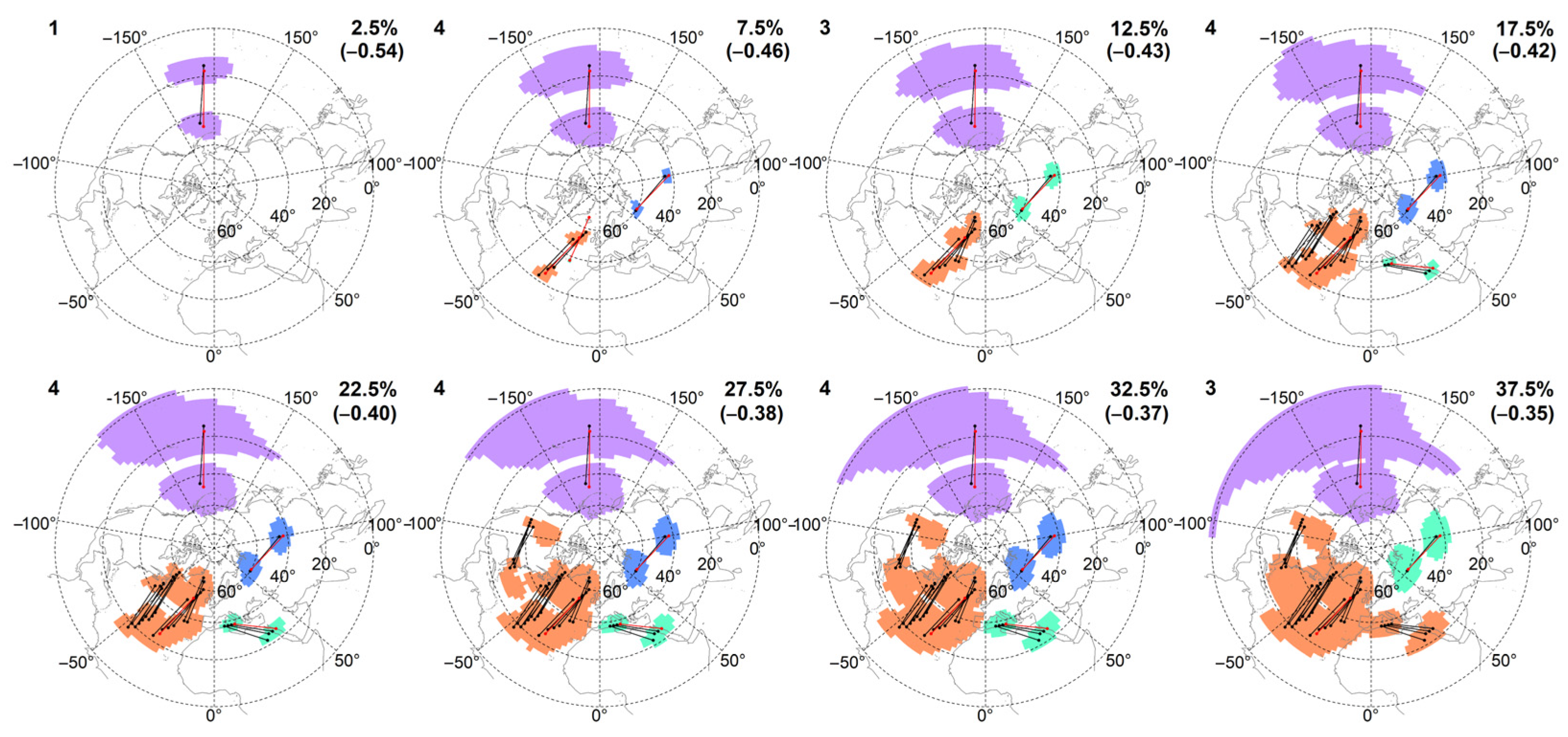
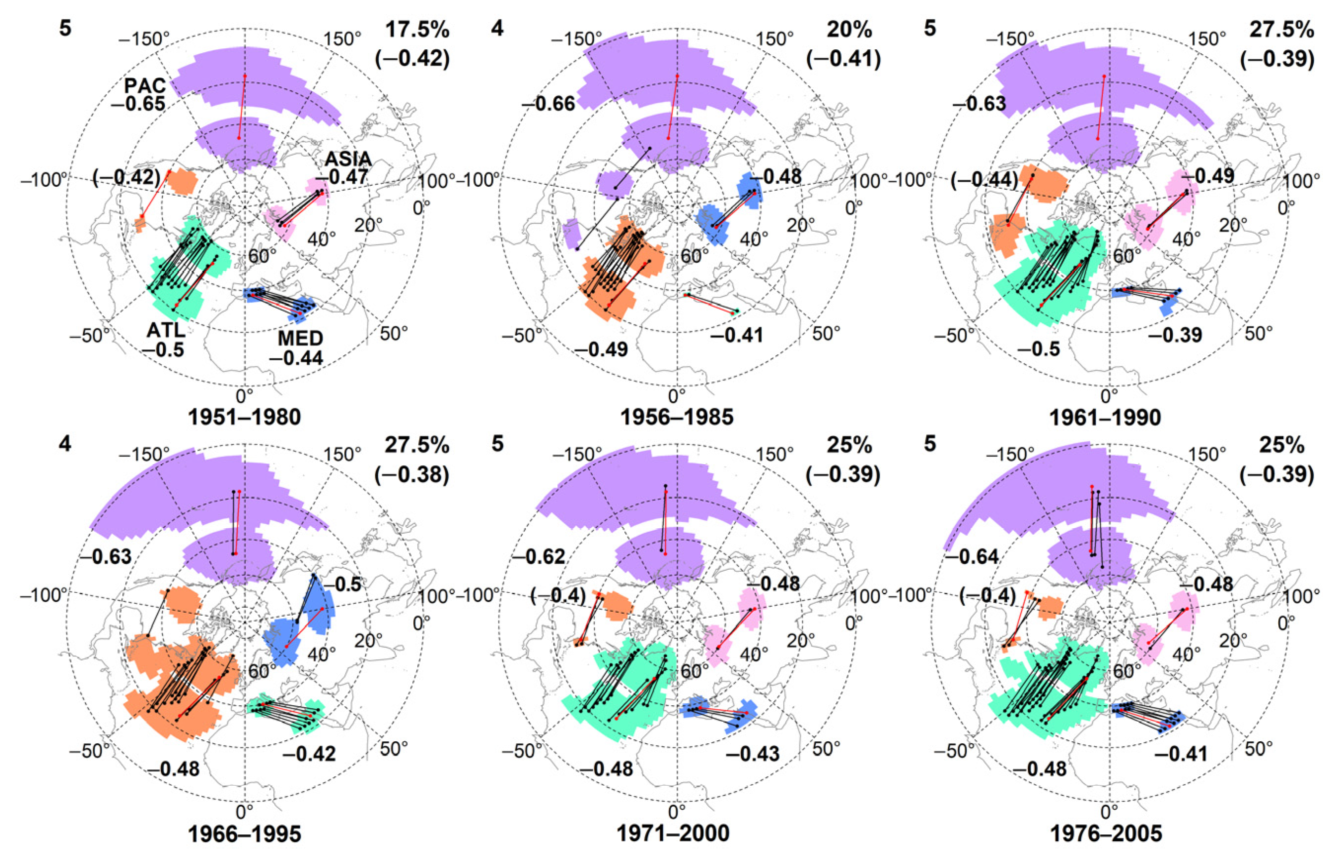
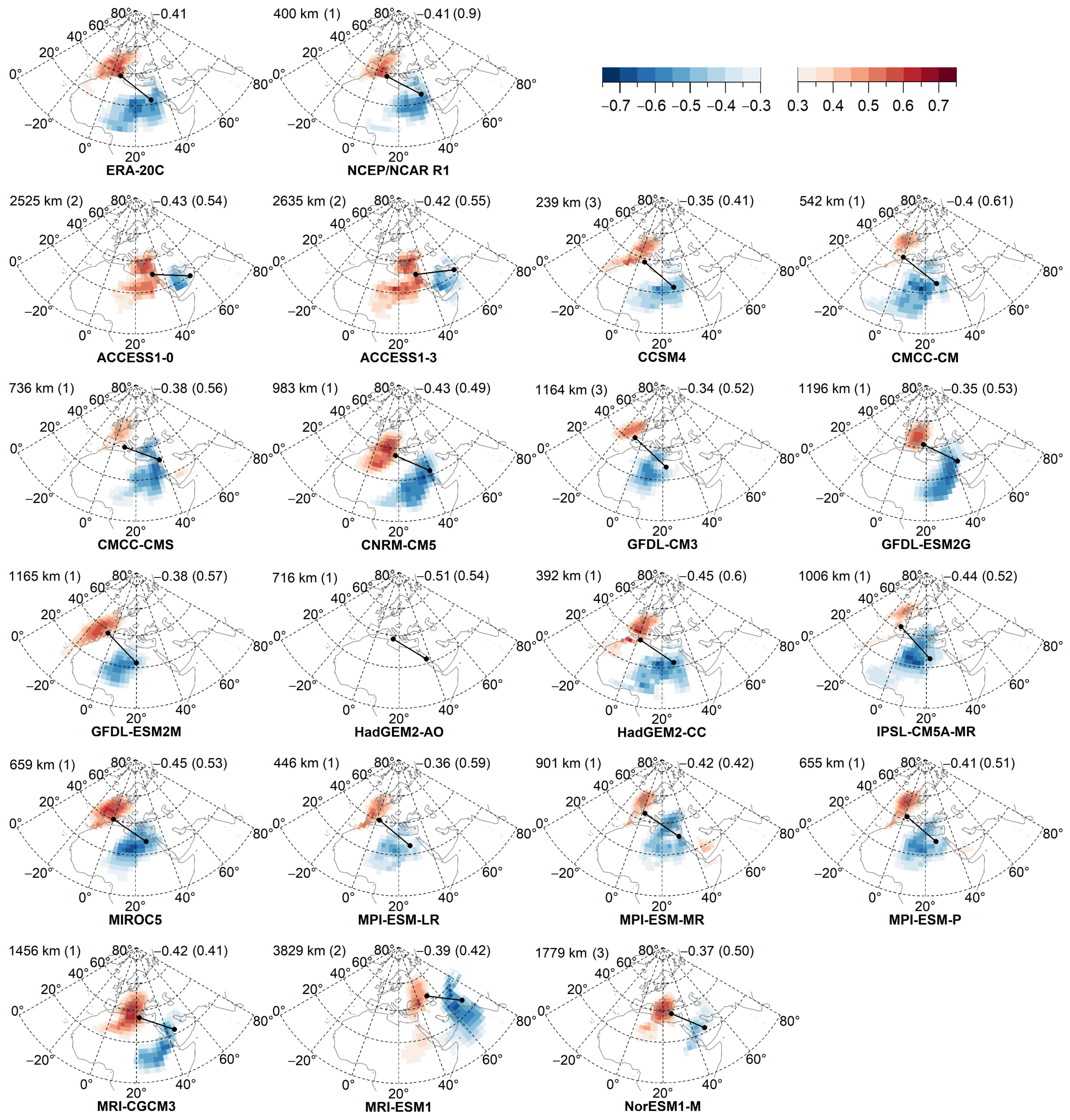
3.1. Selection of the Reference Clusters and Reference CP Maps

As teleconnections are quasi-stationary standing waves, the CP maps obtained from the reanalyses with the most frequently observable clusters are considered to be the imprint of the hemispherical teleconnection patterns. Consequently, at first the occurrence of the clusters was examined in the CP maps of the ERA-20C to determine the reference clusters. The CP map with the lowest threshold was chosen as reference CP map in each time period that contains the reference clusters simultaneously. To support our findings, frequencies of the clusters obtained from NCEP/NCAR R1 were also analyzed.
Based on all CP maps obtained from both reanalyses, a total of 4–7 clusters can be detected in the six examined time periods. At first, the reference CP maps were determined. The reference clusters are located over the North Pacific Ocean (PAC), over the North Atlantic Ocean (ATL), in the regions of the Mediterranean Sea, the Red Sea, and North Africa (MED), and over the West Siberian Plain and the Gobi Desert (ASIA).
The cluster PAC is observable in all CP maps (6 × 39). This cluster is associated with the most intense negative correlations. The cluster ASIA with less intense correlations can be detected in 19–22 CP maps and 16–22 CP maps in each time period of the ERA-20C and the NCEP/NCAR R1, respectively, while the cluster ATL is observable in 17–20 CP maps and 14–18 CP maps of the two reanalyses, except in the period 1956–1985. In this period, the cluster ATL is merged with the cluster PAC at a very low threshold. The cluster MED is associated with the least intense correlations, which makes it the least frequently observable cluster. Before it merges with the cluster ATL, it can be detected in 5–11 CP maps (ERA-20C) and 6–10 CP maps (NCEP/NCAR R1) in five time periods. In the period 1976–2005, it is observable only in two CP maps obtained from both reanalyses.
In all cases, the formation of the cluster ATL, which covers most of the North Atlantic Ocean, is preceded by the appearance of two clusters over the easterly and westerly parts of this region. These two clusters merge at a low threshold. However, those clusters can be separately identified in three CP maps in the period 1976–2005. Concerning the cluster ATL, easterly located grid cells are always associated with more intense correlations than are westerly located grid cells in both reanalyses. Consequently, this cluster is represented with the easterly located pair of ACs in our examination.
Based on the frequencies listed above, the clusters ATL, PAC, MED, and ASIA were chosen as reference clusters, and the reference CP maps are presented in Figure 2.

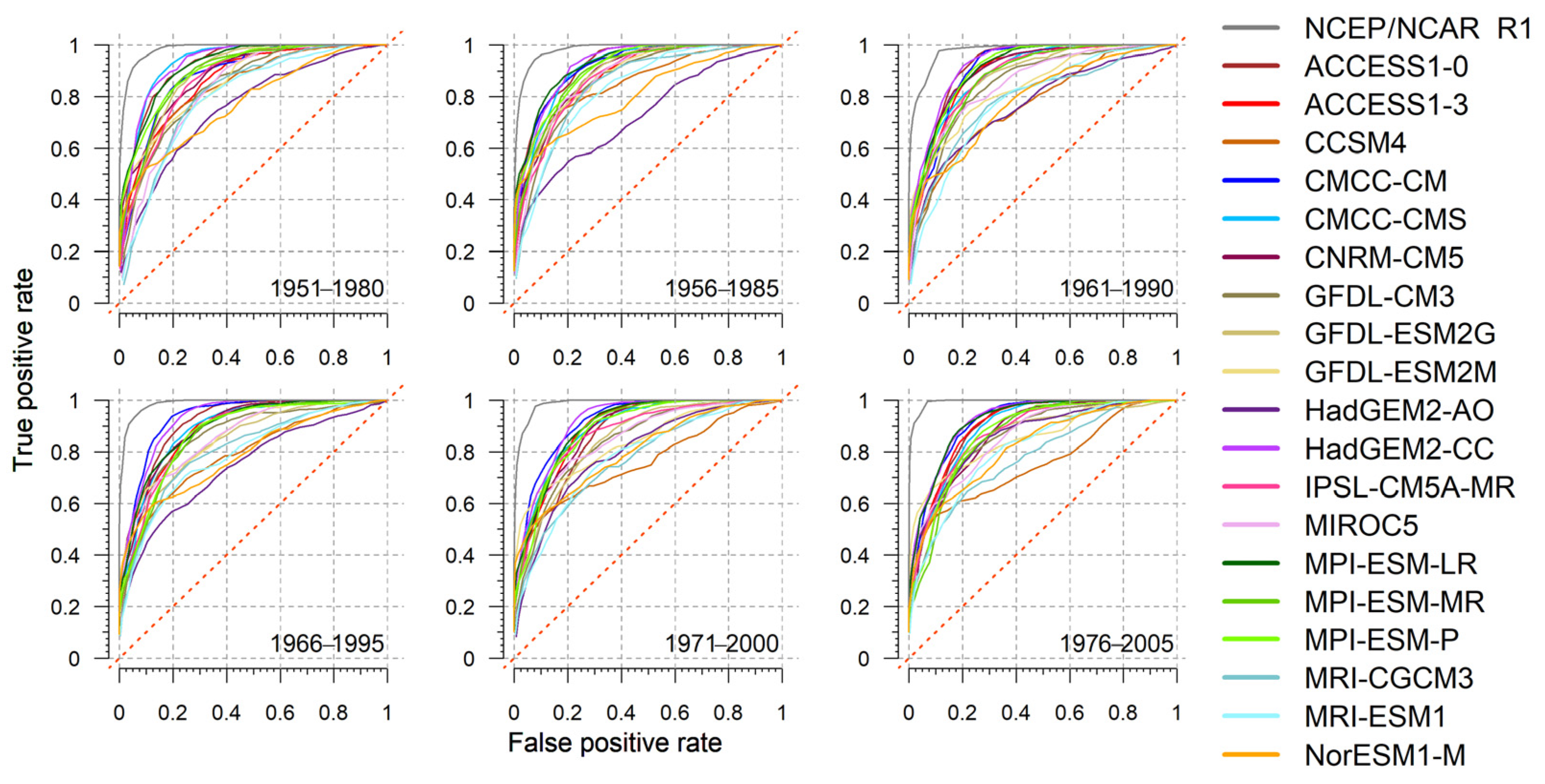
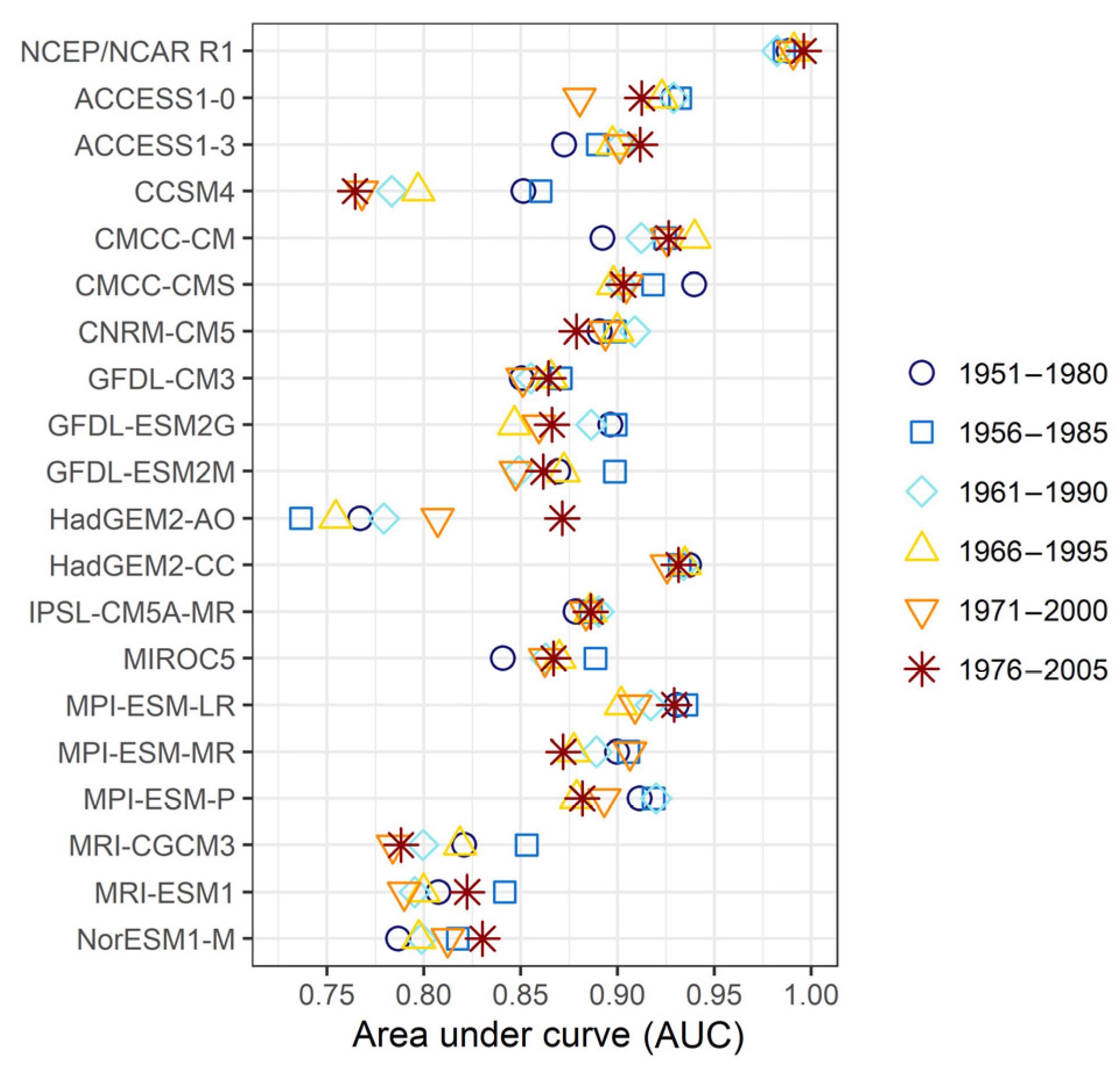
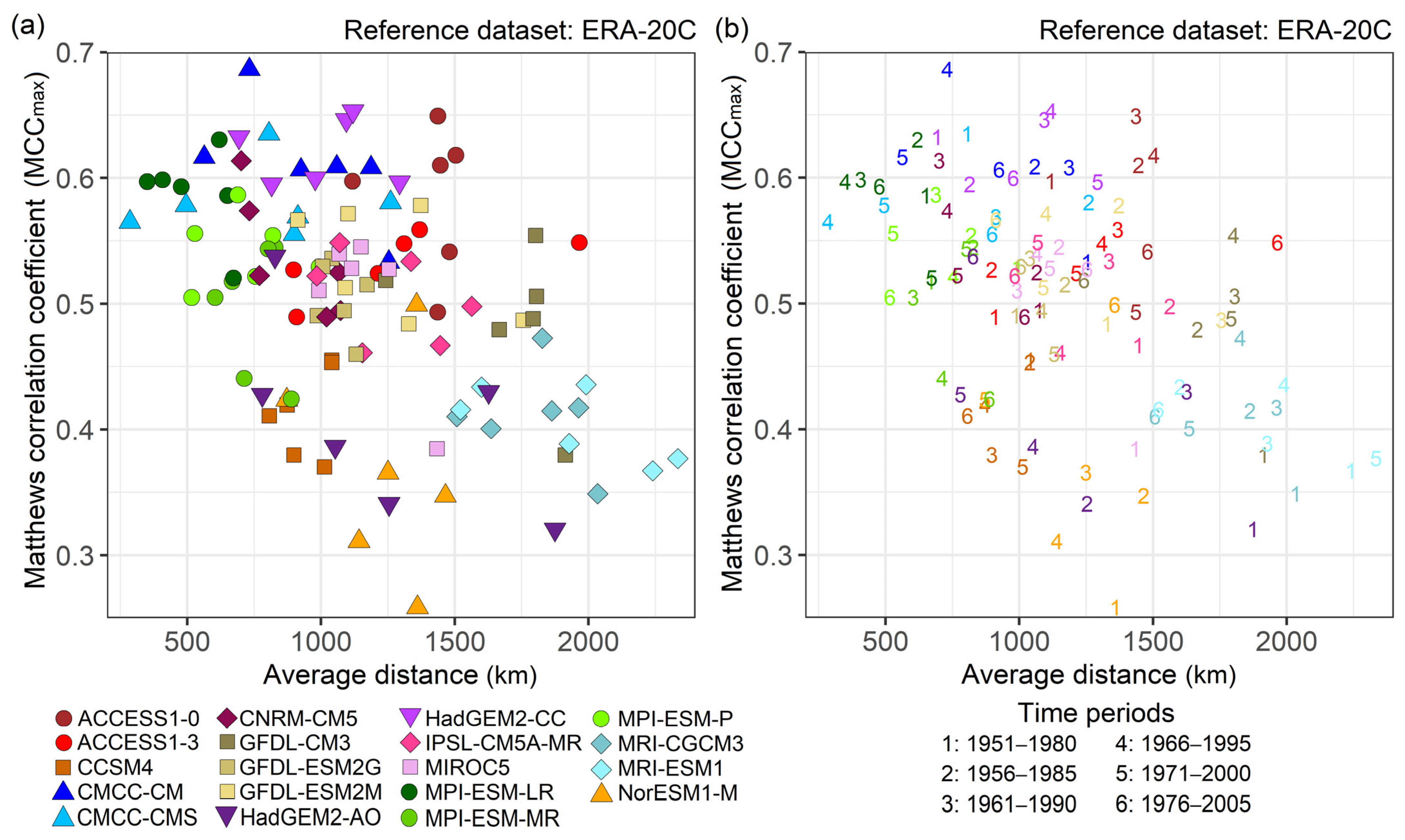
3.2. Results of the AUC-Based Evaluation of the GCMs

The ROC curves of the NCEP/NCAR R1 and the 19 CMIP5 GCMs are shown in Figure 3 for all time periods. The majority of the ROC curves are closely located to each other, while “outliers” can be detected in every time period. However, there is no ROC curve that would imply random GCM performance as all curves are steeper than 45°.
The AUC values associated with each time period are summarized in Figure 4 (the FPR, the TPR, and the AUC values are available in Tables S2–S4 of the Supplementary Material).
Based on the AUC values obtained from the ROC curves, we gain an insight into the hemispherical model performance. The two reanalyses are very similar (AUC > 0.97). The majority of the GCMs are associated with AUC values between 0.8 and 0.95. The small interval implies that GCMs are very similar to each other. On average, AUC values around 0.9 or above 0.9 are associated with the ACCESS1-0, the ACCESS1-3, the CMCC-CM, the CMCC-CMS, the CNRM-CM5, the HadGEM2-CC, the MPI-ESM-LR, and with the MPI-ESM-P. AUC values around 0.8 were computed in cases of the CCSM4, the HadGEM2-AO, the MRI-CGCM3, the MRI-ESM1, and the NorESM1-M.
The average AUC values obtained from all GCMs are around 0.88 in each examined time period, indicating no significant differences in the GCM performance through time. However, there are GCMs where AUC values are higher close to the Millennium, e.g., the ACCESS1-3, the CMCC-CM, and the HadGEM2-AO, while the opposite is observable in cases of the ACCESS1-0, the CMCC-CMS, the GFDL-ESM2G, and the MPI-ESM-P.

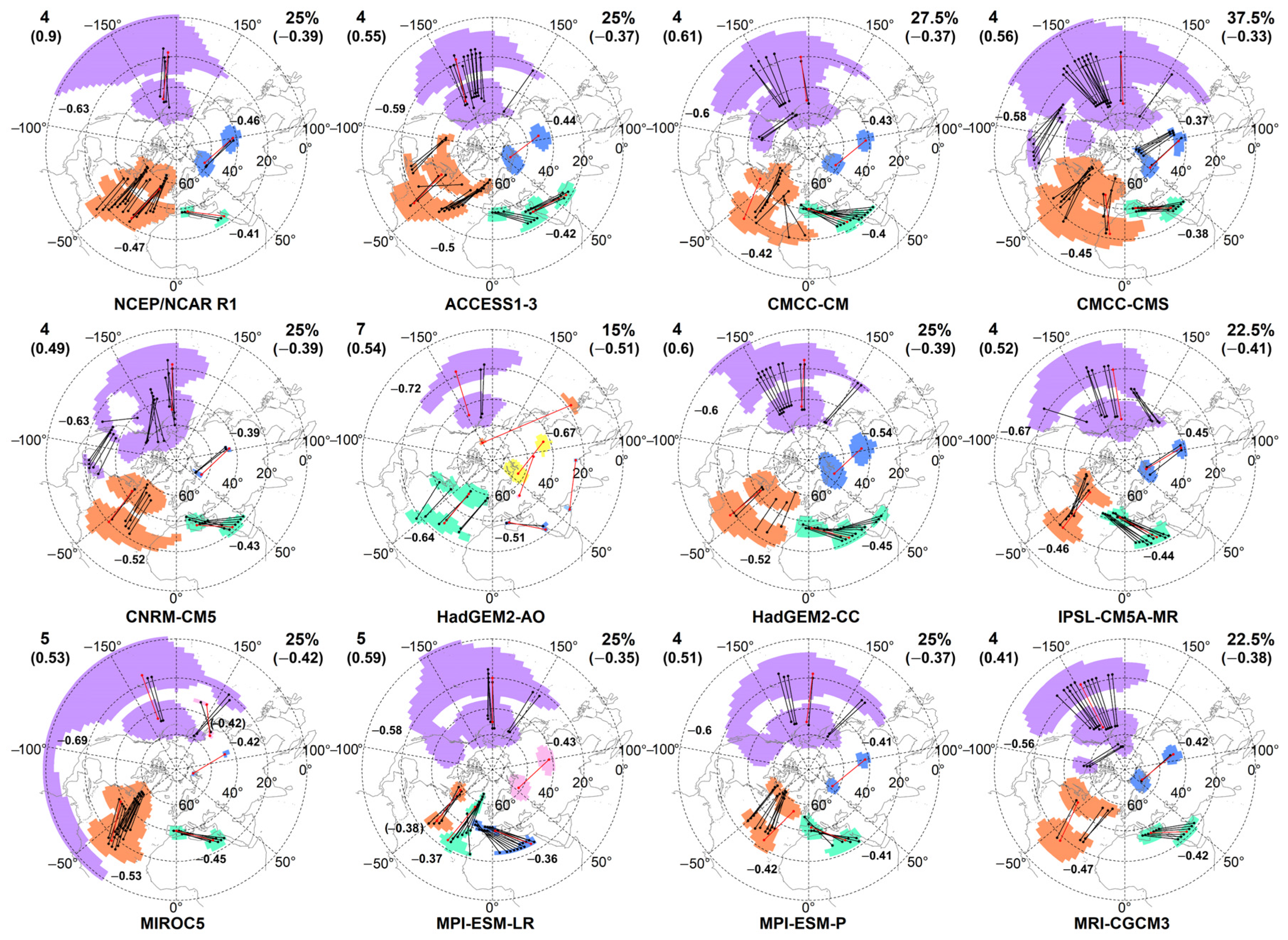
3.3. Results of the Cluster-Based Evaluation of the GCMs

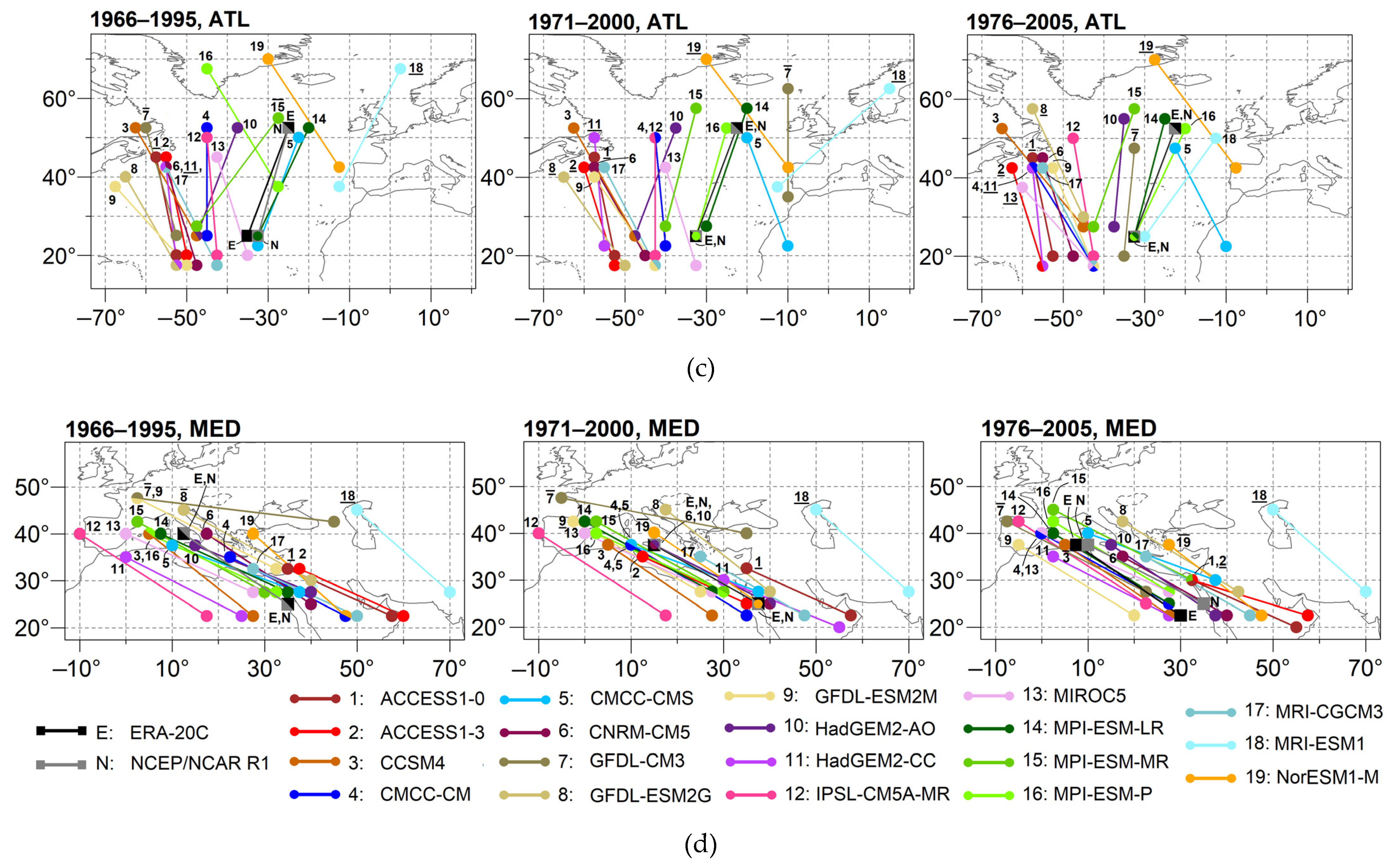
3.3.1. Selection of the Most Similar CP Maps and Matching GCM Clusters with the Reference Clusters

After information is gained about the geographical pattern and number of clusters (i.e., teleconnections), it is possible to benchmark the GCMs regarding their ability to reproduce the observed clusters.
For all 19 GCMs in the six time periods (hereinafter referred to as 114 cases), 4–11 clusters can be detected, except the GFDL-CM3 (in the period 1951–1980 when the number of clusters is three) and the HadGEM2-AO (in the periods of 1961–1990 and 1966–1995 when the number of clusters is 18). A maximum of eight clusters is observable in the same CP map. Therefore, the most similar CP maps were chosen based on the examination of the first three, the first four, etc., the first eight most frequently observable clusters in accordance with the method described in Section 2.2.3. The most similar CP maps are presented in Figure S1 in the Supplementary Material, while an excerpt is shown in Figure 5.
While the clusters obtained from the NCEP/NCAR R1 and the GCMs were matched with the reference clusters based on their frequencies and average distances, three relevant types of the clusters were found (the clusters which are the most similar to the four reference clusters are hereinafter referred to as corresponding clusters). Type 1 indicates that the corresponding cluster in the most similar CP map is among the most frequent and the nearest to the reference cluster. Type 2 means that the corresponding cluster in the most similar CP map is among the most frequently observable clusters, but it is not the nearest cluster. Type 3 indicates that the cluster is not among the most frequently observable clusters, but it is still the nearest cluster. Types of the corresponding clusters and their summary are shown in Tables S6 and S7 of the Supplementary Material.
Based on the types described above, the most similar CP maps can be distinguished from each other, which can be seen in Table 3. The most similar CP maps of the NCEP/NCAR R1 contain only type 1 clusters, except in the period 1956–1985. In this period, the reference cluster ATL can be matched with one of the most frequently observable and nearest clusters obtained from the NCEP/NCAR R1, but there is no CP map in which the cluster ATL is observable with clusters PAC and MED simultaneously (this is the largest discrepancy between the two reanalyses in our examination).
Regarding the GCMs, the following has to be highlighted. In accordance with Table S7 of the Supplementary Material, the case of the GFDL-CM3 in the period 1951–1980 is unique as only three clusters are observable based on the 39 CP maps. Therefore, no cluster can be matched with the reference cluster MED. The corresponding clusters of the CNRM-CM5 belong to type 1 in all time periods, which is also exceptional. If only the last three 30-year-long time periods are examined from 1966 to 2005, then the CMCC-CM, the CMCC-CMS, the HadGEM2-AO, the IPSL-CM5A-MR, the MPI-ESM-LR, the MPI-ESM-P, and the MRI-CGCM3 are added to this list. As the corresponding clusters PAC and ASIA belong to type 1 in 114 and 113 cases, the above-described means that in cases of clusters ATL and MED, more corresponding clusters belong to type 1 in the last three examined time periods than in the first three examined time periods.
According to Figure S1 of the Supplementary Material, the following conclusions can be drawn. The NCEP/NCAR R1 produces similarly distributed teleconnections (i.e., the clusters PAC, ATL, MED, and ASIA) as the ERA-20C does in all time periods. The largest discrepancy is observable for the period 1956–1985, mentioned above. Most of the GCMs can reproduce the same distribution of teleconnections as the reanalyses (e.g., the CNRM-CM5 and the HadGEM2-CC in all time periods). The most frequent types of errors are summarized below. Some GCMs tend to do the following:
  • Simulate the teleconnections over the Pacific Ocean more easterly compared to the ERA-20C (e.g., the GFDL-CM3 and the MIROC5), while most of the GCMs do not capture this shift.
  • Reproduce the atmospheric bridge between the Atlantic Ocean and the Pacific Ocean more often than the ERA-20C does (e.g., the CCSM4, the GFDL-CM3, and the MRI-ESM1; the NCEP/NCAR R1 in the period 1956–1985).
  • Represent the teleconnection patterns over the North Atlantic Ocean with two distinct clusters (e.g., in some periods of the CMCC-CMS and the MPI-ESM-LR).
  • Simulate the most intense regions of the teleconnections over the Atlantic Ocean more westerly than the ERA-20C does (e.g., the ACCESS1-0, the ACCESS1-3, the CCSM4, and the HadGEM2-AO).
  • Capture the ACs of cluster ATL in a north-eastern position similar to those of the ERA-20C but reproduce a cluster with more intense correlations over the western part of the North Atlantic Ocean. This cluster merges with the cluster PAC at a low threshold before the easterly located cluster pops up (e.g., in cases of the MRI-ESM1 and the NorESM1-M).
  • Miss the cluster MED from the CP map (e.g., the GFDL-CM3 for the period 1951–1980), or the clusters ATL and MED form a joint cluster (e.g., in some time periods of the CMCC-CM, the CMCC-CMS, and the IPSL-CM5A-MR).
  • Locate the most intense regions of the cluster MED more easterly than those of the ERA-20C (e.g., the MRI-CGCM3, and the MRI-ESM1) or reproduce two intensity centers in this area, which leads to altering ACs depending on the examined time period (e.g., the ACCESS1-0, the ACCESS1-3, and the HadGEM2-CC).

3.3.2. Evaluation of the GCMs with Respect to the Geographical Location of the ACs

In the following, we gain further insight into the GCM performance based on the analysis of the ACs of the corresponding GCM clusters. In order to conduct the analysis, ACs of type 1 clusters were taken into account. If those were not available, then ACs obtained from type 2 clusters were used. In case of type 3 clusters, the ACs of the nearest clusters relative to the given reference cluster were applied. Average distances of the two poles of the teleconnections represented with the clusters PAC, ATL, MED, and ASIA are summarized in Table 4.
Regarding the cluster PAC, an easterly shift of the ACs can be seen from 1951 to 2005 in both reanalyses (3–4 grid cells in case of the ERA-20C and 2–3 grid cells in case of the NCEP/NCAR R1), as it can be seen in Figure 6a. However, most of the GCMs cannot capture this shift. Exceptions are the NorESM1-M and the GFDL-CM3. Other GCMs relocate the ACs with a few grid cells westerly, e.g., the CMCC-CM, the CMCC-CMS, the CNRM-CM5, the MIROC5, and the MRI-CGCM3. As a consequence, the MIROC5 and the MRI-CGCM3 seem to be more accurate considering temporal evolution, as the average distance decreases closer to the Millennium. It is important to recognize that it is only the consequence of those GCMs failing to represent the observed easterly shift.
The average distances associated with the cluster ASIA obtained from the GCMs are the smallest among all the four clusters. However, GCM ACs are typically located with a few grid cells northerly to the ACs of the reference cluster. While the GCMs are the most accurate in this region, as shown in Figure 6b, the differences between the two reanalyses are the largest in this cluster among all the four clusters. In the period 1951–1980, the ACs obtained from the NCEP/NCAR R1 are located north-easterly/easterly to the ACs of the ERA-20C. However, the difference between the two reanalyses decreases with time.
Due to the merging of the clusters ATL and MED at a low threshold (which restricts the separate examination), only the last three time periods are shown in Figure 6c,d, when the ACs obtained from most of the GCMs are relatively stable. The discrepancies between most of the GCMs and the reanalyses in case of the cluster ATL originate from the GCMs that simulate stronger correlations over the north-western part of the Atlantic Ocean, while the reanalyses capture the more intense correlations over the north-eastern region. Consequently, those GCMs are unable to capture the easterly shift of the teleconnection over the north-eastern part of the Atlantic Ocean, which can be detected in both reanalyses. The MPI-ESM-LR, the MPI-ESM-MR, and the MPI-ESM-P reproduce the cluster in the north-eastern part of the oceanic area in similar position to that of the reanalyses.
In case of the MED cluster, an easterly shift is also observable concerning the reanalyses. This tendency is not easily captured as some of the GCMs falsely reproduce two intensity centers in this area. GCMs such as the CNRM-CM5, the HadGEM2-AO, and the NorESM1-M reproduce the ACs in a more stable position than the reanalyses do. Even there are GCMs in which westerly shift is observable, such as the MPI-ESM-LR, the MPI-ESM-MR, and the MPI-ESM-P. In these GCMs the connection between the clusters ATL and MED become more pronounced closer to the Millennium. If the first three 30-year-long time periods are compared to the last three periods, then a slight decrease in the average distances is observable. On average, the GCMs perform the most accurately concerning the teleconnection represented with the cluster ASIA. It is followed by the clusters PAC and MED where the inaccuracies derive from the uncertainty listed above.

3.3.3. Synthesis

The importance of the MCCmax values lies in the fact that they support the selection of the GCM CP maps that are the most similar to those of the ERA-20C. However, it can also be used as a metric to evaluate GCMs as it measures not only the GCM’s ability to reproduce teleconnections but also those regions taken into account by the MCCmax where no teleconnection is observable. Therefore, the performance of the GCMs is quantified by the MCCmax values and the average distances computed based on all four reference clusters. The corresponding results are presented in Figure 7. In order to calculate the average distances, the four corresponding clusters are taken into account in case of each GCM in each time period, except for the GFDL-CM3 in the period 1951–1980 when only three clusters can be examined.
The highest MCCmax values are associated with the NCEP/NCAR R1 between 0.8 and 0.9. In almost 90% of all cases, the MCCmax values obtained from the GCMs vary in a narrow interval, between 0.3 and 0.6. This means that no GCM performs exceptionally well over the whole NH. This is in line with the shortcomings concerning the GCMs listed above. The variance of the MCCmax values decreases with time. Regarding the geographical position of the ACs, the GCMs are more accurate concerning clusters PAC and ASIA while those are less precise in cases of clusters ATL and MED.
According to the results, the model families like CMCC and the MRI are located in similar regions of the plot presented in Figure 7. Based on the MCCmax values and the average distance, more information is gained about the GCM performance compared to when using the AUC values. The structure of the teleconnections and their ACs was reproduced the most accurately in cases of the CMCC-CM, the CMCC-CMS, the MPI-ESM-LR, and the MPI-ESM-MR in the periods of 1966–1995, 1971–2000, and 1976–2005. High (low) MCCmax values do not necessarily imply small (large) average distances, which can be exemplified with the HadGEM2-CC (CCSM4).
Increasing AUC or MCCmax values and decreasing average distances with time (e.g., in cases of the HadGEM2-AO) can imply improvement or just coincidence, as it can be seen in case of cluster PAC. The latter can be taken into consideration by examining the position of the ACs.
The following types of models can be distinguished in accordance with Figure 7: GCMs with relatively high (~0.6) MCCmax values and small (~500 km) average distances (e.g., the MPI-ESM-LR); GCMs with high MCCmax values and moderate (750–1000 km) average distances (e.g., the CMCC-CM and the HadGEM2-CC); GCMs with low (~0.4) MCCmax values and moderate average distances (e.g., the CCSM4); furthermore, GCMs with low MCCmax values and large (1250–1500 km) average distances (e.g., the GFDL-CM3 and the MRI-ESM1).

3.3.4. Construction of Mobile Teleconnection Indices

The analysis of the ACs enables us to explore connections between the large-scale circulation and atmospheric variables. In Figure 8, correlations are presented between the air temperature anomalies at 2 m (t2m) and the mobile teleconnection index defined as the H500 difference of the westerly and easterly located ACs of the cluster MED. This index can be considered a mobile MO index. The Mediterranean region is one of the “future meteorological drought hot spots” as more severe and frequent droughts are expected until 2100 [8]. These raise the importance of analyzing this region. In this example, t2m was chosen because it can be easily downloaded in cases of all GCMs. In addition to the two reanalyses, the correlations of all GCMs are plotted.
The most intense regions of the teleconnections are in the vicinity of the ACs. Therefore, differences between the correlation fields obtained from the GCMs and those of the reanalyses are expected to increase with increasing average distances regarding the cluster MED. Positive correlations close to the westerly located AC mean higher (lower) than average H500, which is associated with higher (lower) than average t2m. Negative correlations indicate higher (lower) than average H500 in the vicinity of the westerly located AC and lower (higher) than average t2m close to the easterly located AC.
In Figure 8, average distance concerns only the cluster MED. The performance of the GCMs varies in a relatively large range (239–3829 km), while the MCCmax values computed over the NH change in a small interval (0.41–0.61). The GCMs with relatively small average distances can reproduce the correlation field similarly to the ERA-20C (e.g., the CMCC-CMS, the HadGEM2-CC, the MPI-ESM-LR, and the MPI-ESM-P). The GCMs with relatively large average distances may capture the most intense correlations in different regions (e.g., in cases of the ACCESS1-0, the ACCESS1-3, the MRI-CGCM3, and the MRI-ESM1). If the GCM clusters are similarly located to the reference clusters but there are large discrepancies outside of those areas, then realistic reproduction of the relation between teleconnections and atmospheric variables is not guaranteed. The HadGEM2-AO can be mentioned as an example, which failed to capture significant correlations between the t2m field and the mobile teleconnection index.

4. Discussion

Policy-relevant assessment of the impact of climate change by analyzing future scenarios by GCMs is a crucial task. Based on proper estimations, adaption strategies can be elaborated, which may support decision-makers [86]. Because of this, the quality of GCM outputs has to be continuously evaluated. As teleconnections are related to the large-scale flows in the atmosphere (e.g., Rossby wave; the geographical location of high/low pressure systems), their examination provides a benchmark to capture errors in the GCMs.
In this study, we used a complex pattern detection methodology to localize clusters in the H500 field that describe the geographical location of teleconnections in the Northern Hemisphere. For the examination, 30-year-long periods were chosen because teleconnec-tions can be detected with more geographically fixed nodes on a longer time scale than on a shorter time scale [87]. As a reference, the ERA-20C reanalysis dataset was chosen because it is considered the state-of-the-art realization of the atmospheric processes with sufficient temporal coverage. Using the NCEP/NCAR R1 to corroborate our results was also beneficial. It bears similarity with the ERA-20C, and those two datasets are recom-mended as references by Stryhal and Huth [88]. Similarities between the two reanalyses regarding the H500 field were also confirmed by Kristóf et al. [51].
In line with the teleconnections detected by Wallace and Gutzler [19], Wallace and Blackmon [25], and Conte et al. [27], the cluster PAC corresponds to the Pacific/North American (PNA) pattern. The cluster ATL implies the West Atlantic (WA) and the East Atlantic (EA) patterns simultaneously. Furthermore, the clusters MED and ASIA indicate the Mediterranean Oscillation (MO) and the Eurasia (EU) patterns. Representing the WA and the EA patterns with a single cluster is realistic as those are not independent phenom-ena [19]. In our pattern detection algorithm, every cluster consists of two ACs. Consequently, the four poles of the PNA (i.e., over the Pacific Ocean and North America) are not connected. However, a “bridge” between the clusters PAC and ATL is observable from 1956 to 1985 in both reanalyses. That is reasonable as the PNA and the WA patterns are not independent phenomena [19]. The regions of the North Atlantic Ocean and the Mediterranean Sea are also not independent from each other [89,90]. Local correlation minima—which correspond to teleconnections in the SNC fields—are surrounded with significant negative correlations. Those make it impossible to delimit teleconnections unequivocally [19,25,51]. The pattern detection algorithm described in Section 2.2.1 is applicable to delimit teleconnections in an automatized way if the threshold of the SNCs is given.
To assess the uncertainty of the GCM performance, the analysis of an ensemble of GCMs is advised [52]. Therefore, numerous studies draw consequences from examining the ensemble of the CMIP5 GCM (e.g., [42,46]). In the present study, we sought to determine significant changes in the GCM performance and to avoid the construction of fluctuating GCM rankings. In order to reach that goal, an ensemble of cluster patterns was created and a pattern detection algorithm was applied to the SNC fields in a deterministic way. The proposed clustering algorithm is preferred over clustering algorithms such as k-medoid or k-means methods because the results of those techniques are not always convergent. If those are applied, then different CP maps will be obtained if the clustering method is repeated. This problem can be resolved by smoothing the SNC fields before the clustering, but it requires the estimation of the optimal smoothing parameter. The preservation of the PotACs is also questionable as those are faded by the smoothing. With our proposed method, those problems can be avoided.
The ROC curve analysis has been used since the 1950s in the fields of biostatistics to measure the performance of diagnostic tests (e.g., [91]). In 1989, the World Meteorological Organization (WMO) proposed this method for the validation of climate predictions and weather forecasts [92]. The method has growing popularity in the field of atmospheric studies. Mason and Graham [93] used ROC curve analysis to validate forecast skill of GCMs concerning rainfall over the eastern part of Africa. Shin et al. [94] used it to evaluate the forecast performance of a hydrological drought model. De Castro Santos et al. [95] classified the intensities of El Niño episodes by applying ROC technique. ROC curve analysis proved to be an effective way to compare binary-coded CP maps.
Crucial steps of the ROC curve-based GCM evaluation were the selection of the reference CP maps and the threshold. The latter is associated with the GCM CP map, which is the most similar to the reference CP map in case of each GCM in each time period. The distribution of the correlation values of the SNC fields slightly changes in time (Table S1 in the Supplementary Material) and depends on the selected reanalyses/GCMs. Consequently, the thresholds depend on the analyzed time period. Furthermore, different summary measures (e.g., the Youden index [91] and the MCC [75]) can be applied (a detailed summary of those metrics is provided by Schisterman et al. [96]). Similarity to the CP maps depends on the chosen metric. Therefore, it shall be carefully selected. We chose the MCC because it is proper for unbalanced data [75] as the amounts of zero and one values are not equal in the CP maps.
The ACs obtained from the SNC fields may serve as the basis for constructing tele-connection indices. As climate indices, those are important tools to explore climate change signals as they reflect variability of the large-scale circulation. For instance, numerous indices are available in the North Atlantic and Mediterranean regions (e.g., [26,27,28,29,30]). Recently, a growing number of climate indices are available in various fields of climatology—e.g., human thermal comfort indices [97,98,99]—which can be easily accessed, e.g., in packages of the R programming language [100]. We should emphasize that there is an ongoing debate whether station-based/grid-point-based teleconnection indices (referred to as regional indices) or PC-based indices express more information of atmospheric variability. According to Kutzbach [21], PC-based indices express less information than do regional indices but they carry more information than zonal indices, which are based on hemispherical average fields. The mobile NAO index constructed by Portis et al. [31] correlated better with observations than did the PC-based and station-based indices. On the contrary, Kuzmina et al. [101] concluded that PC-based indices gave more information about the distribution of the pressure field than did station-based indices. Criado-Aldeanueva and Soto-Navarro [32] pointed out that the PC-based MO index obtained from air pressure correlated better with precipitation and evaporation time series in the Mediterranean region if the whole year was considered. However, in winter, when large-scale atmospheric processes dominate over smaller-scale processes, regional indices also capture atmospheric variability realistically. The authors consider that pairs of ACs obtained from the SNC fields represent the most intense regions of the teleconnections properly due to the dependency in the SNC fields. It ensures that not only pairs of ACs but also neighboring grid cells are associated with similarly strong correlations.
In our analysis, GCMs reproduced the ACs of clusters PAC and ASIA accurately relative to the ERA-20C. The ACs are in less accurate positions in cases of clusters ATL and MED. However, GCMs are less accurate in capturing the eastward shift of the ACs of the clusters ATL and PAC in the last decades of the 20th century. The eastward shift detected in the reanalyses can be in line with the eastward shift of the teleconnections near the surface, which was described by Hilmer and Jung [102] and Favre and Gershunov [103].
Finally, we emphasize that the AUC and MCCmax values are not proper by themselves to select the best-performing GCMs relative to the ERA-20C concerning the spatial structure of the teleconnection. The examination of the ACs is also crucial, which can be exemplified with the HadGEM2-CC (Figure 5 and Figure 8). Despite the relatively high MCCmax values, the most similar CP maps obtained from the HadGEM2-CC fail to capture the most intense regions of the clusters ATL and MED in some time periods. Because the GCM performs well otherwise, relatively high AUC and MCCmax values are associated with it. Dissimilarities are quantified with the average distances, which indicate large differences between the ACs obtained from the HadGEM2-CC and those from the ERA-20C. Thus, if mobile teleconnection indices are constructed based on the ACs of the clusters ATL and MED, then those indices will represent different areas compared to the reanalysis.

5. Conclusions

In the current study, a complex evaluation of GCMs was presented with respect to the spatial structure of atmospheric teleconnections. The novel feature of the study is that teleconnections were delimited in an automatized way without arbitrary (subjective) area selection. The threshold obtained from the given SNC field was the only parameter that has to be set by the user. Consequently, GCMs can be evaluated in each time period, which enables us to track temporal changes in the GCM performance. The evaluation method is considered to be an extension to the method of Kristóf et al. [51] in which stability of teleconnections was examined based on two ensembles (those ensembles were constructed of the SNC fields of 30-year-long and 10-year-long time periods).
Similarities of the GCMs relative to the reference dataset can be assessed with the AUC value obtained from the ROC curve on the hemispherical level. By computing the MCCmax values and the average distances, we gain further insight into the cluster structure of the reanalyses and the GCMs. Examination of the ACs allowed us to distinguish real temporal improvement in the GCM performance from random changes. Therefore, we avoided creating GCM rankings that are associated with random fluctuations.
We emphasize that the interpretation of the results obtained from statistical methods always contains subjective elements [12]. In order to choose the reference CP maps and the summary measures (i.e., MCC), human considerations were taken into account, i.e., whether or not the obtained patterns express relevant physical meaning. Otherwise, the proposed method is free from arbitrary decisions.
We demonstrated that all examined CMIP5 GCMs could capture the most prominent teleconnections in the winter atmospheric circulation of the NH, especially in the periods closer to the Millennium. The CMCC-CM, the CMCC-CMS, the HadGEM2-CC, the MPI-ESM-LR, and the MPI-ESM-P are considered the most reliable GCMs in line with the findings of Kristóf et al. [51]. The GCMs can reproduce the ACs over Asia very accurately. However, it is important to recognize that even the above-mentioned GCMs failed to reproduce eastward shifts of the ACs over the North Pacific Ocean and the North Atlantic Ocean. Some GCMs reproduce the WA with enhanced intensity compared to the EA, or fail to reproduce the monopolar correlation structure in the SNC fields over the Mediterranean region. According to our findings, there is no connection between the model performance and horizontal resolution of the GCMs. However, most of the GCMs with a well-resolved stratosphere are among the best performing GCMs.
Finally, we encourage the use of the above-described method (1) to evaluate other GCM generations (especially CMIP6 GCMs and forthcoming Earth system models), (2) to carry out regional studies, and (3) to construct additional mobile teleconnection indices to explore relations between teleconnections and atmospheric variables. Results obtained from the correlations between the mobile MO index and t2m fields are promising. Therefore, comprehensive analysis with other variables is the subject of a forthcoming publication.
The codes and the calculated datasets are available from the first author upon request.

Supplementary Materials

The following are available online at www.mdpi.com/article/10.3390/atmos12101236/s1, Figure S1: The maps of cluster patterns (CP maps) obtained from the NCEP/NCAR R1, and the CMIP5 GCMs. Table S1: Percentile values of the SNCs below which correlations are taken into account to create CP maps; Table S2: False positive rates (FPR) in case of each CP map associated with the percentile values between 2.5 and 95; Table S3: True positive rates (TPR) in case of each CP map associated with the percentile values between 2.5 and 95; Table S4: Area under curve (AUC) values; Table S5: Values of the Matthews correlation coefficients (MCC); Table S6: Details of the action centers (AC). Table S7. Examination of the corresponding clusters. Table S8. Summary table of the maximum values of the Matthews correlation coefficients (MCCmax) and average distances (km).

Author Contributions

Conceptualization, E.K., R.H., Z.B., R.P. and J.B.; methodology, E.K. and R.H.; software, E.K. and R.H.; validation, E.K.; formal analysis, E.K.; investigation, E.K.; resources, E.K. and Z.B.; data curation, E.K.; writing—original draft preparation, E.K. and Z.B.; writing—review and editing, E.K., Z.B. and R.P.; visualization, E.K.; supervision, Z.B.; project administration, Z.B., R.P., J.B. and E.K; funding acquisition, Z.B., R.P. and J.B. All authors have read and agreed to the published version of the manuscript.

Funding

The research has been supported by the Széchenyi 2020 program, the European Regional Development Fund, the Hungarian Government (GINOP-2.3.2-15-2016-00028) and by the Hungarian National Research, Development and Innovation Fund (K-129162 and K-120605). Z.B. is supported by grant “Advanced research supporting the forestry and wood-processing sector’s adaptation to global change and the 4th industrial revolution”, No. CZ.02.1.01/0.0/0.0/16_019/0000803 financed by OP RDE.

Informed Consent Statement

Not applicable.

Data Availability Statement

Data of the CMIP5 GCM outputs were downloaded from the Earth System Grid Federation (ESGF) node: https://esgf-data.dkrz.de/search/cmip5-dkrz/ (accessed on 9 May 2021). The ERA-20C data were accessed on the website: https://apps.ecmwf.int/datasets/data/era20c-daily/levtype=pl/type=an/ (accessed on 9 May 2021), while the NCEP/NCAR R1 data can be downloaded from the following website: https://psl.noaa.gov/data/gridded/data.ncep.reanalysis.pressure.html (accessed on 9 May 2021).

Acknowledgments

We acknowledge the World Climate Research Program’s Working Group on Coupled Modeling, which is responsible for CMIP, and we thank the climate modeling groups for producing and making available their model output. The NCEP/NCAR Reanalysis 1 data are provided by the NOAA/OAR/ESRL PSD, Boulder, CO, USA. The ERA-20C data are provided by the ECMWF. We thank the two anonymous reviewers for the useful notes and comments.

Conflicts of Interest

The authors declare no conflict of interest.

References

  1. United Nations. Adoption of the Paris Agreement. Framework Convention on Climate Change; FCCC/CP/2015/L.9/Rev.1; UN: Paris, France, 2015; Available online: https://unfccc.int/resource/docs/2015/cop21/eng/l09r01.pdf (accessed on 9 May 2021).
  2. James, R.; Washington, R.; Schleussner, C.-F.; Rogelj, J.; Conway, D. Characterizing half-a-degree difference: A review of methods for identifying regional climate responses to global warming targets. Clim. Chang. 2017, 8, e457. [Google Scholar] [CrossRef] [Green Version]
  3. Dosio, A.; Mentaschi, L.; Fischer, E.M.; Wyser, K. Extreme heat waves under 1.5 °C and 2 °C global warming. Environ. Res. Lett. 2018, 13, 054006. [Google Scholar] [CrossRef] [Green Version]
  4. Samaniego, L.; Thober, S.; Kumar, R.; Wanders, N.; Rakovec, O.; Pan, M.; Zink, M.; Sheffield, J.; Wood, E.F.; Marx, A. Anthropogenic warming exacerbates European soil moisture droughts. Nat. Clim. Chang. 2018, 8, 421–426. [Google Scholar] [CrossRef]
  5. Sun, Q.; Miao, C.; Hanel, M.; Borthwick, A.G.L.; Duan, Q.; Ji, D.; Li, H. Global heat stress on health, wildfires, and agricultural crops under different levels of climate warming. Environ. Int. 2019, 128, 125–136. [Google Scholar] [CrossRef] [PubMed]
  6. Gaupp, F.; Hall, J.; Mitchell, D.; Dadson, S. Increasing risks of multiple breadbasket failure under 1.5 and 2 °C global warming. Agric. Syst. 2019, 175, 34–45. [Google Scholar] [CrossRef] [Green Version]
  7. IPCC. Summary for Policymakers. In Global Warming of 1.5 °C; An IPCC Special Report on the impacts of Global Warming of 1.5 °C above Pre-Industrial Levels and Related Global Greenhouse Gas Emission Pathways, in the Context of Strengthening the Global Response to the Threat of Climate Change, Sustainable Development, and Efforts to Eradicate Poverty; Masson-Delmotte, V., Zhai, P., Pörtner, H.-O., Roberts, D., Skea, J., Shukla, P.R., Pirani, A., Moufouma-Okia, W., Péan, C., Pidcock, R., et al., Eds.; IPCC: Geneva, Switzerland, 2018; 24p, in press. [Google Scholar]
  8. Spinoni, J.; Barbosa, P.; Bucchignani, E.; Cassano, J.; Cavazos, T.; Christensen, J.H.; Christensen, O.B.; Coppola, E.; Evans, J.; Geyer, B.; et al. Future Global Meteorological Drought Hot Spots: A Study Based on CORDEX Data. J. Clim. 2020, 33, 3635–3661. [Google Scholar] [CrossRef]
  9. Field, C.B.; Barros, T.F.; Stocker, D.; Qin, D.J.; Dokken, K.L.; Ebi, M.D.; Mastrandrea, K.J.; Mach, G.-K.; Plattner, S.K.; Tignor, A.M.; et al. (Eds.) Managing the Risks of Extreme Events and Disasters to Advance Climate Change Adaptation. A Special Report of Working Groups I and II of the Intergovernmental Panel on Climate Change; Cambridge University Press: Cambridge, UK; New York, NY, USA, 2012; p. 582. [Google Scholar]
  10. Matthews, T.K.R.; Wilby, R.L.; Murphy, C. Communicating the deadly consequences of global warming for human heat stress. Proc. Natl. Acad. Sci. USA 2017, 114, 3861–3866. [Google Scholar] [CrossRef] [PubMed] [Green Version]
  11. IPCC–Climate Change 2013: The Physical Science Basis. In Contribution of Working Group I to the Fifth Assessment Report of the Intergovernmental Panel on Climate Change; Cambridge University Press: Cambridge, UK; New York, NY, USA, 2013; p. 1535.
  12. Horel, J.D. A Rotated Principal Component Analysis of the Interannual Variability of the Northern Hemisphere 500 mb Height Field. Mon. Weather Rev. 1981, 109, 2080–2092. [Google Scholar] [CrossRef] [Green Version]
  13. Opsteegh, J.D.; Van den Dool, H.M. Seasonal Differences in the Stationary Response of a Linearized Primitive Equation Model: Prospects for Long-Range Weather Forecasting? J. Atmos. Sci. 1980, 37, 2169–2185. [Google Scholar] [CrossRef] [Green Version]
  14. Hoskins, B.J.; Karoly, D.J. The Steady Linear Response of a Spherical Atmosphere to Thermal and Orographic Forcing. J. Atmos. Sci. 1981, 38, 1179–1196. [Google Scholar] [CrossRef] [Green Version]
  15. Kornhuber, K.; Osprey, S.; Coumou, D.; Petri, S.; Petoukhov, V.; Rahmstorf, S.; Gray, L. Extreme weather events in early summer 2018 connected by a recurrent hemispheric wave-7 pattern. Environ. Res. Lett. 2019, 14, 054002. [Google Scholar] [CrossRef]
  16. Fragkoulidis, G.; Wirth, V.; Bossmann, P.; Fink, A.H. Linking Northern Hemisphere temperature extremes to Rossby wave packets. Q. J. R. Meteorol. Soc. 2018, 144, 553–566. [Google Scholar] [CrossRef]
  17. Ward, P.J.; Jongman, B.; Kummu, M.; Dettinger, M.D.; Sperna Weiland, F.C.; Winsemius, H.C. Strong influence of El Niño Southern Oscillation on flood risk around the world. Proc. Natl. Acad. Sci. USA 2014, 111, 15659–15664. [Google Scholar] [CrossRef] [PubMed] [Green Version]
  18. Gaupp, F.; Hall, J.; Hochrainer-Stigler, S.; Dadson, S. Changing risks of simultaneous global breadbasket failure. Nat. Clim. Chang. 2020, 10, 54–57. [Google Scholar] [CrossRef]
  19. Wallace, J.M.; Gutzler, D.S. Teleconnections in the Geopotential Height Field during the Northern Hemisphere Winter. Mon. Weather Rev. 1981, 109, 784–812. [Google Scholar] [CrossRef]
  20. Barnston, A.G.; Livezey, R.E. Classification, Seasonality and Persistence of Low-Frequency Atmospheric Circulation Patterns. Mon. Weather Rev. 1987, 115, 1083–1126. [Google Scholar] [CrossRef]
  21. Kutzbach, J.E. Large-scale features of monthly mean Northern Hemisphere anomaly maps of sea-level pressure. Mon. Weather Rev. 1970, 98, 708–716. [Google Scholar] [CrossRef]
  22. Mo, K.C.; Livezey, R.E. Tropical-Extratropical Geopotential Height Teleconnections during the Northern Hemisphere Winter. Mon. Weather Rev. 1986, 114, 2488–2515. [Google Scholar] [CrossRef]
  23. Cheng, X.; Wallace, J.M. Cluster Analysis of the Northern Hemisphere Wintertime 500-hPa Height Field: Spatial Patterns. J. Atmos. Sci. 1993, 50, 2674–2696. [Google Scholar] [CrossRef] [Green Version]
  24. Küttel, M.; Luterbacher, J.; Wanner, H. Multidecadal changes in winter circulation-climate relationship in Europe: Frequency variations, within-type modifications, and long-term trends. Clim. Dyn. 2011, 36, 957–972. [Google Scholar] [CrossRef] [Green Version]
  25. Wallace, J.M.; Blackmon, M.L. Observations of low-frequency atmospheric variability. In Large-Scale Dynamical Processes in the Atmosphere; Hoskins, B.J., Pearce, R.P., Eds.; Academic Press: New York, NY, USA, 1983; pp. 55–94. [Google Scholar]
  26. Rogers, R. The Association between the North Atlantic Oscillation and the Southern Oscillation in the Northern Hemisphere. Mon. Weather Rev. 1984, 112, 1999–2015. [Google Scholar] [CrossRef]
  27. Conte, M.; Giuffrida, A.; Tedesco, S. The Mediterranean Oscillation, Impact on Precipitation and Hydrology in Italy. In Conference on Climate Water; Academy of Finland: Helsinki, Finland, 1989; pp. 121–137. [Google Scholar]
  28. Hurrell, J.W. Decadal Trends in the North Atlantic Oscillation: Regional Temperatures and Precipitation. Science 1995, 269, 676–679. [Google Scholar] [CrossRef] [Green Version]
  29. Brunetti, M.; Maugeri, M.; Nanni, T. Atmospheric circulation and precipitation in Italy for the last 50 years. Int. J. Climatol. 2002, 22, 1455–1471. [Google Scholar] [CrossRef]
  30. Palutikof, J.P. Analysis of Mediterranean climate data: Measured and modelled. In Mediterranean Climate: Variability and Trends; Bolle, H.J., Ed.; Springer: Berlin, Germany, 2003; pp. 125–132. [Google Scholar]
  31. Portis, D.H.; Walsh, J.E.; El Hamly, M.; Lamb, P.J. Seasonality of the North Atlantic Oscillation. J. Clim. 2001, 14, 2069–2078. [Google Scholar] [CrossRef]
  32. Criado-Aldeanueva, F.; Soto-Navarro, F.J. The Mediterranean Oscillation teleconnection index: Station-based versus principal component paradigms. Adv. Meteorol. 2013, 738501. [Google Scholar] [CrossRef] [Green Version]
  33. Taylor, K.E. Summarizing multiple aspects of model performance in a single diagram. J. Geophys. Res. 2001, 106, 7183–7192. [Google Scholar] [CrossRef]
  34. Gleckler, P.J.; Taylor, K.E.; Doutriaux, C. Performance metrics for climate models. J. Geophys. Res. 2008, 113, D06104. [Google Scholar] [CrossRef]
  35. Charlton-Perez, A.J.; Baldwin, M.P.; Birner, T.; Black, R.X.; Butler, A.H.; Calvo, N.; Davis, N.A.; Gerber, E.P.; Gillett, N.; Hardiman, S.; et al. On the lack of stratospheric dynamical variability in low-top versions of the CMIP5 models. J. Geophys. Res. Atmos. 2013, 118, 2494–2505. [Google Scholar] [CrossRef]
  36. Seviour, J.M.; Gray, L.J.; Mitchell, D.M. Stratospheric polar vortex splits and displacements in the high-top CMIP5 climate models. J. Geophys. Res. Atmos. 2016, 121, 1400–1413. [Google Scholar] [CrossRef] [Green Version]
  37. Marsland, S.J.; Bi, D.; Uotila, P.; Fiedler, R.; Griffies, S.M.; Lorbacher, K.; O’Farrell, S.; Sullivan, A.; Uhe, P.; Zhou, X.; et al. Evaluation of ACCESS climate model ocean diagnostics in CMIP5 simulations. Aust. Meteorol. Oceanogr. J. 2013, 63, 101–119. [Google Scholar] [CrossRef]
  38. Caesar, L.; Rahmstorf, S.; Robinson, A.; Feulner, G.; Saba, V. Observed fingerprint of a weakening Atlantic Ocean overturning circulation. Nature 2018, 556, 191–196. [Google Scholar] [CrossRef]
  39. Rashid, H.A.; Sullivan, A.; Hirst, A.C.; Bi, D.; Zhou, X.; Marsland, S.J. Evaluation of El Niño–Southern Oscillation in the ACCESS coupled model simulations for CMIP5. Aust. Meteorol. Oceanogr. J. 2013, 63, 161–180. [Google Scholar] [CrossRef]
  40. Lu, Z.; Fu, Z.; Hua, L.; Yuan, N.; Chen, L. Evaluation of ENSO simulations in CMIP5 models: A new perspective based on percolation phase transition in complex networks. Sci. Rep. 2018, 8, 14912. [Google Scholar] [CrossRef] [Green Version]
  41. Zuo, J.-Q.; Li, W.-J.; Ren, H.-L. Representation of the Arctic Oscillation in the CMIP5 Models. Adv. Clim. Chang. Res. 2013, 4, 242–249. [Google Scholar] [CrossRef]
  42. Bellenger, H.; Guilyardi, E.; Leloup, J.; Lengaigne, M.; Vialard, J. ENSO representation in climate models: From CMIP3 to CMIP5. Clim. Dyn. 2014, 42, 1999–2018. [Google Scholar] [CrossRef]
  43. Davini, P.; Cagnazzo, C. On the misinterpretation of the North Atlantic Oscillation in CMIP5 models. Clim. Dyn. 2014, 43, 1497–1511. [Google Scholar] [CrossRef]
  44. Ning, L.; Bradley, R.S. NAO and PNA influences on winter temperature and precipitation over the eastern United States in CMIP5 GCMs. Clim. Dyn. 2016, 46, 1257–1276. [Google Scholar] [CrossRef]
  45. Belleflamme, A.; Fettweis, X.; Lang, C.; Erpicum, M. Current and future atmospheric circulation at 500 hPa over Greenland simulated by the CMIP3 and CMIP5 global models. Clim. Dyn. 2013, 41, 2061–2080. [Google Scholar] [CrossRef]
  46. Stryhal, J.; Huth, R. Trends in winter circulation over the British Isles and central Europe in twenty-first century projections by 25 CMIP5 GCMs. Clim. Dyn. 2019, 52, 1063–1075. [Google Scholar] [CrossRef]
  47. Stryhal, J.; Huth, R. Classifications of winter atmospheric circulation patterns: Validation of CMIP5 GCMs over Europe and the North Atlantic. Clim. Dyn. 2019, 52, 3575–3598. [Google Scholar] [CrossRef]
  48. Khan, N.; Shahid, S.; Ahmed, K.; Ismail, T.; Nawaz, N.; Son, M. Performance Assessment of General Circulation Model in Simulating Daily Precipitation and Temperature Using Multiple Gridded Datasets. Water 2018, 10, 1793. [Google Scholar] [CrossRef] [Green Version]
  49. Sa’adi, Z.; Shiru, M.S.; Shahid, S.; Ismail, T. Selection of general circulation models for the projections of spatio-temporal changes in temperature of Borneo Island based on CMIP5. Theor. Appl. Climatol. 2020, 139, 351–371. [Google Scholar] [CrossRef]
  50. Kononova, N.K.; Lupo, A.R. Changes in the Dynamics of the Northern Hemisphere Atmospheric Circulation and the Relationship to Surface Temperature in the 20th and 21st Centuries. Atmosphere 2020, 11, 255. [Google Scholar] [CrossRef] [Green Version]
  51. Kristóf, E.; Barcza, Z.; Hollós, R.; Bartholy, J.; Pongrácz, R. Evaluation of Historical CMIP5 GCM Simulation Results Based on Detected Atmospheric Teleconnections. Atmosphere 2020, 11, 723. [Google Scholar] [CrossRef]
  52. Taylor, K.E.; Stouffer, R.J.; Meehl, G.A. An overview of CMIP5 and the Experiment Design. Bull. Am. Meteorol. Soc. 2012, 93, 485–498. [Google Scholar] [CrossRef] [Green Version]
  53. Egger, J. On the theory of the steady perturbations in the troposphere. Tellus 1976, 28, 381–390. [Google Scholar] [CrossRef]
  54. Feldstein, S.B. The dynamics of NAO teleconnection pattern growth and decay. Q. J. R. Meteorol. Soc. 2003, 129, 901–924. [Google Scholar] [CrossRef]
  55. Poli, P.; Herschbach, H.; Dee, D.P.; Berrisford, P.; Simmons, A.J.; Vitart, F.; Laloyaux, P.; Tan, D.G.H.; Peubey, C.; Thépaut, J.-N.; et al. ERA-20C: An Atmospheric Reanalysis of the Twentieth Century. J. Clim. 2016, 29, 4083–4097. [Google Scholar] [CrossRef]
  56. Kalnay, E.; Kanamitsu, M.; Kistler, R.; Collins, W.; Deaven, D.; Gandin, L.; Iredell, M.; Saha, S.; White, G.; Woollen, J.; et al. The NCEP/NCAR 40-Year Reanalysis Project. Bull. Am. Meteorol. Soc. 1996, 77, 437–472. [Google Scholar] [CrossRef] [Green Version]
  57. Bi, D.; Dix, M.; Marsland, S.J.; O’Farrell, S.; Rashid, H.A.; Uotila, P.; Hirst, A.C.; Kowalczyk, E.; Golebiewski, M.; Sullivan, A.; et al. The ACCESS coupled model: Description, control climate and evaluation. Aust. Meteorol. Oceanogr. J. 2013, 63, 41–64. [Google Scholar] [CrossRef]
  58. Gent, P.R.; Danabasoglu, G.; Donner, L.J.; Holland, M.M.; Hunke, E.C.; Jayne, S.R.; Lawrence, D.M.; Neale, R.B.; Rasch, P.J.; Vertenstein, M.; et al. The Community Climate System Model version 4. J. Clim. 2011, 24, 4973–4991. [Google Scholar] [CrossRef]
  59. Scoccimarro, E.; Gualdi, S.; Bellucci, A.; Sanna, A.; Fogli, P.G.; Manzini, E.; Vichi, M.; Oddo, P.; Navarra, A. Effects of Tropical Cyclones on Ocean Heat Transport in a High-Resolution Coupled General Circulation Model. J. Clim. 2011, 24, 4368–4384. [Google Scholar] [CrossRef] [Green Version]
  60. Manzini, E.; Cagnazzo, C.; Fogli, P.G.; Bellucci, A.; Müller, W.A. Stratosphere-troposphere coupling at inter-decadal time scales: Implications for the North Atlantic Ocean. Geophys. Res. Lett. 2012, 39, L05801. [Google Scholar] [CrossRef] [Green Version]
  61. Voldoire, A.; Sanchez-Gomez, E.; Mélia, D.S.; Decharme, B.; Cassou, C.; Sénési, S.; Valcke, S.; Beau, I.; Alias, A.; Chevallier, M.; et al. The CNRM-CM5.1 global climate model: Description and basic evaluation. Clim. Dyn. 2013, 40, 2091–2121. [Google Scholar] [CrossRef] [Green Version]
  62. Donner, L.J.; Wyman, B.L.; Hemler, R.S.; Horowitz, L.W.; Ming, Y.; Zhao, M.; Golaz, J.-C.; Ginoux, P.; Lin, S.-J.; Schwarzkopf, M.D.; et al. The Dynamical Core, Physical Parameterizations, and Basic Simulation Characteristics of the Atmospheric Component AM3 of the GFDL Global Coupled Model CM3. J. Clim. 2011, 24, 3484–3519. [Google Scholar] [CrossRef]
  63. Dunne, J.P.; John, J.G.; Adcroft, A.J.; Griffies, S.M.; Hallberg, R.W.; Shevliakova, E.; Stouffer, R.J.; Cooke, W.; Dunne, K.A.; Harrison, M.J.; et al. GFDL’s ESM2 Global Coupled Climate–Carbon Earth System Models. Part I: Physical Formulation and Baseline Simulation Characteristics. J. Clim. 2012, 25, 6646–6665. [Google Scholar] [CrossRef] [Green Version]
  64. Dunne, J.P.; John, J.G.; Shevliakova, E.; Stouffer, R.J.; Krasting, J.P.; Malyshev, S.; Milly, P.C.D.; Sentman, L.T.; Adcroft, A.J.; Cooke., W.; et al. GFDL’s ESM2 Global Coupled Climate–Carbon Earth System Models. Part II: Carbon System Formulation and Baseline Simulation Characteristics. J. Clim. 2013, 26, 2247–2267. [Google Scholar] [CrossRef] [Green Version]
  65. Martin, G.M.; Bellouin, N.; Collins, W.J.; Culverwell, I.D.; Halloran, P.R.; Hardiman, S.C.; Hinton, T.J.; Jones, C.D.; McDonald, R.E.; McLaren, A.J.; et al. The HadGEM2 family of Met Office Unified Model climate configurations. Geosci. Model Dev. 2011, 4, 723–757. [Google Scholar] [CrossRef] [Green Version]
  66. Dufresne, J.-L.; Foujols, M.-A.; Denvil, S.; Caubel, A.; Marti, O.; Aumont, O.; Balkanski, Y.; Bekki, S.; Bellenger, H.; Benshila, R.; et al. Climate change projections using the IPSL-CM5 Earth System Model: From CMIP3 to CMIP5. Clim. Dyn. 2013, 40, 2123–2165. [Google Scholar] [CrossRef]
  67. Watanabe, M.; Suzuki, T.; O’Ishi, R.; Komuro, Y.; Watanabe, S.; Emori, S.; Takemura, T.; Chikira, M.; Ogura, T.; Sekiguchi, M.; et al. Improved climate simulation by MIROC5: Mean states, variability, and climate sensitivity. J. Clim. 2010, 23, 6312–6335. [Google Scholar] [CrossRef]
  68. Raddatz, T.J.; Reick, C.H.; Knorr, W.; Kattge, J.; Roeckner, E.; Schnur, R.; Schnitzler, K.-G.; Wetzel, P.; Jungclaus, J. Will the tropical land biosphere dominate the climate–carbon cycle feedback during the twenty-first century? Clim. Dyn. 2007, 29, 565–574. [Google Scholar] [CrossRef]
  69. Jungclaus, J.H.; Lorenz, S.J.; Timmreck, C.; Reick, C.H.; Brovkin, V.; Six, K.; Segschneider, J.; Giorgetta, M.A.; Crowley, T.J.; Pongratz, J.; et al. Climate and carbon-cycle variability over the last millennium. Clim. Past 2010, 6, 723–737. [Google Scholar] [CrossRef] [Green Version]
  70. Yukimoto, S.; Yoshimura, H.; Hosaka, M.; Sakami, T.; Tsujino, H.; Hirabara, M.; Tanaka, T.Y.; Deushi, M.; Obata, A.; Nakano, H.; et al. Meteorological Research Institute-Earth System Model Version 1 (MRI-ESM1)—Model Description. Tech. Rep. Meteorol. Res. Inst. 2011, 64, 83. [Google Scholar] [CrossRef]
  71. Adachi, Y.; Yukimoto, S.; Deushi, M.; Obata, A.; Nakano, H.; Tanaka, T.Y.; Hosaka, M.; Sakami, T.; Yoshimura, H.; Hirabara, M.; et al. Basic performance of a new earth system model of the Meteorological Research Institute. Pap. Meteorol. Geophys. 2013, 64, 1–19. [Google Scholar] [CrossRef] [Green Version]
  72. Iversen, T.; Bentsen, M.; Bethke, I.; Debernard, J.B.; Kirkevåg, A.; Seland, Ø.; Drange, H.; Kristjansson, J.E.; Medhaug, I.; Sand, M.; et al. The Norwegian Earth System Model, NorESM1-M—Part 2: Climate response and scenario projections. Geosci. Model Dev. 2012, 5, 2933–2998. [Google Scholar] [CrossRef]
  73. Bentsen, M.; Bethke, I.; Debernard, J.B.; Iversen, T.; Kirkevåg, A.; Seland, Ø.; Drange, H.; Roelandt, C.; Seierstad, I.A.; Hoose, C.; et al. The Norwegian Earth System Model, NorESM1-M—Part 1: Description and basic evaluation of the physical climate. Geosci. Model Dev. 2013, 6, 687–720. [Google Scholar] [CrossRef] [Green Version]
  74. Zou, K.H.; O’Malley, A.J.; Mauri, L. Receiver-Operating Characteristic Analysis for Evaluating Diagnostic Tests and Predictive Models. Circulation 2007, 115, 654–657. [Google Scholar] [CrossRef] [Green Version]
  75. Chicco, D.; Jurman, G. The advantages of the Matthews correlation coefficient (MCC) over F1 score and accuracy in binary classification evaluation. BMC Genom. 2020, 21, 6. [Google Scholar] [CrossRef] [Green Version]
  76. Schulzweida, U. CDO User Guide (Version 1.9.8); Max Planck Institute for Meteorology: Hamburg, Germany, 2019. [Google Scholar] [CrossRef]
  77. R Core Team. R: A Language and Environment for Statistical Computing; R Foundation for Statistical Computing: Vienna, Austria, 2020; Available online: http://www.R-project.org/ (accessed on 15 August 2021).
  78. Pierce, D. ncdf4: Interface to Unidata NetCDF (Version 4 or Earlier) Format Data Files. R Package Version 1.16. 2019. Available online: https://CRAN.R-project.org/package=ncdf4 (accessed on 15 August 2021).
  79. Wickham, H. ggplot2: Elegant Graphics for Data Analysis; Springer: New York, NY, USA, 2016. [Google Scholar]
  80. Nychka, D.; Furrer, R.; Paige, J.; Sain, S. Fields: Tools for Spatial Data. R Package Version 9.9. 2017. Available online: https://cran.r-project.org/web/packages/fields/index.html (accessed on 15 August 2021). [CrossRef]
  81. Brownrigg, R.; Minka, T.P.; Deckmyn, A. Maps: Draw Geographical Maps. R Package Version 3.3.0. Original S Code by R.A. Becker, A.R. Wilks. 2018. Available online: https://CRAN.R-project.org/package=maps (accessed on 15 August 2021).
  82. Bivand, R.; Lewin-Koh, N. Maptools: Tools for Handling Spatial Objects. R Package Version 0.9-4. 2018. Available online: https://CRAN.R-project.org/package=maptools (accessed on 15 August 2021).
  83. McIlroy, D. Packaged for R by Brownrigg, R., Minka. T.P. Transition to Plan 9 Codebase by Bivand. R. Mapproj: Map Projections. R Package Version 1.2.6. 2018. Available online: https://CRAN.R-project.org/package=mapproj (accessed on 15 August 2021).
  84. Neuwirth, E. RColorBrewer: ColorBrewer Palettes. R Package Version 1.1-2. 2014. Available online: https://CRAN.R-project.org/package=RcolorBrewer (accessed on 15 August 2021).
  85. Ooms, J. Magick: Advanced Graphics and Image-Processing in R. R Package Version 2.5.1. 2020. Available online: https://CRAN.R-project.org/package=magick (accessed on 15 August 2021).
  86. Pokovai, K.; Hollós, R.; Bottyán, E.; Kis, A.; Marton, T.; Pongrácz, R.; Pásztor, L.; Hidy, D.; Barcza, Z.; Fodor, N. Estimation of agro-ecosystem services using biogeochemical models. Q. J. Hung. Meteorol. Serv. 2020, 124, 209–225. [Google Scholar] [CrossRef]
  87. Kushnir, Y.; Wallace, J.M. Low-Frequency Variability in the Northern Hemisphere Winter: Geographical Distribution, Structure and Time-Scale Dependence. J. Atmos. Sci. 1989, 46, 3122–3143. [Google Scholar] [CrossRef] [Green Version]
  88. Stryhal, J.; Huth, R. Classifications of Winter Euro-Atlantic Circulation Patterns: An Intercomparison of Five Atmospheric Reanalyses. J. Clim. 2017, 30, 7847–7861. [Google Scholar] [CrossRef]
  89. Dünkeloh, A.; Jacobeit, J. Circulation Dynamics of Mediterranean Precipitation Variability 1948–98. Int. J. Climatol. 2003, 23, 1843–1866. [Google Scholar] [CrossRef]
  90. Criado-Aldeanueva, F.; Soto-Navarro, F.J.; García-Lafuente, J. Large-Scale Atmospheric Forcing Influencing the Long-Term Variability of Mediterranean Heat and Freshwater Budgets: Climatic Indices. J. Hydrometeorol. 2014, 15, 650–663. [Google Scholar] [CrossRef]
  91. Youden, W.J. Index for rating diagnostic tests. Cancer 1950, 3, 32–35. [Google Scholar] [CrossRef]
  92. Stanski, H.R.; Wilson, L.J.; Burrows, W.R. Survey of Common Verification Methods in Meteorology; WMO World Weather Watch Technical Report No.8, WMO/TD No. 358; Atmospheric Environment Service Forecast Research Division: Geneve, Switzerland, 1989. [Google Scholar]
  93. Mason, S.J.; Graham, N.E. Conditional Probabilities, Relative Operating Characteristics, and Relative Operating Levels. Weather Forecast. 1999, 14, 713–725. [Google Scholar] [CrossRef]
  94. Shin, J.Y.; Kwon, H.-H.; Lee, J.-H.; Kim, T.-W. Probabilistic long-term hydrological drought forecast using Bayesian networks and drought propagation. Meteorol. Appl. 2020, 27, e1827. [Google Scholar] [CrossRef] [Green Version]
  95. De Castro Santos, M.A.; Vega-Oliveros, D.A.; Zhao, L.; Berton, L. Classifying El Niño-Southern Oscillation Combining Network Science and Machine Learning. IEEE Access 2020, 8, 55711–55723. [Google Scholar] [CrossRef]
  96. Schisterman, E.F.; Faraggi, D.; Reiser, B.; Hu, J. Youden Index and the optimal threshold for markers with mass at zero. Stat. Med. 2008, 27, 297–315. [Google Scholar] [CrossRef] [Green Version]
  97. Höppe, P. The physiological equivalent temperature—A universal index for the biometeorological assessment of the thermal environment. Int. J. Biometeorol. 1999, 43, 71–75. [Google Scholar] [CrossRef]
  98. Błażejczyk, K.; Jendritzky, G.; Bröde, P.; Fiala, D.; Havenith, G.; Epstein, Y.; Psikuta, A.; Kampmann, B. An Introduction to the Universal Thermal Climate Index (UTCI). Geogr. Pol. 2013, 86, 5–10. [Google Scholar] [CrossRef] [Green Version]
  99. Ács, F.; Kristóf, E.; Zsákai, A.; Kelemen, B.; Szabó, Z.; Marques Vieira, L.A. Weather in the Hungarian Lowland from the Point of View of Humans. Atmosphere 2021, 12, 84. [Google Scholar] [CrossRef]
  100. Charalampopoulos, I. The R Language as a Tool for Biometeorological Research. Atmosphere 2020, 11, 682. [Google Scholar] [CrossRef]
  101. Kuzmina, S.I.; Bengtsson, L.; Johannessen, O.M.; Drange, H.; Bobylev, L.P.; Miles, M.W. The North Atlantic Oscillation and greenhouse-gas forcing. Geophys. Res. Lett. 2005, 32, L04703. [Google Scholar] [CrossRef] [Green Version]
  102. Hilmer, M.; Jung, T. Evidence for a recent change in the link between the North Atlantic Oscillation and Arctic sea ice export. Geophys. Res. Lett. 2000, 27, 989–992. [Google Scholar] [CrossRef] [Green Version]
  103. Favre, A.; Gershunov, A. Extra-tropical cyclonic/anticyclonic activity in North-Eastern Pacific and air temperature extremes in Western North America. Clim. Dyn. 2006, 26, 617–629. [Google Scholar] [CrossRef]
Figure 1. CP maps obtained from the ERA-20C for the period 1971–2000 over the NH. Each cluster is plotted with different color. The PotACs are visualized with black dots connected with black lines. (On average, 40 PotACs with an associated correlation below −0.3 can be obtained in each period). The PotAC with the most intense SNC in each cluster is highlighted with red. The numbers of clusters can be found in the top-left corner of the maps. The percentile of all SNCs and its value (below which the SNCs are taken into account to create the CP map) are shown in the top-right corner of each map. The associated data are available in Table S1 of the Supplementary Material. The SNC fields with the PotACs of the reanalyses and the GCMs in all time periods and a selection of CPs obtained from the reanalyses and the GCMs are available from the first author upon request.
Atmosphere 12 01236 g001
Figure 2. Reference CP maps obtained from the ERA-20C for the six time periods used in the study. The four reference clusters are texted in the CP map on the top-left corner of the figure. The correla-tions associated with the ACs (denoted with red dots connected with red lines) are provided on the maps, next to the clusters. Interpretation of the maps is similar to that of Figure 1.
Atmosphere 12 01236 g002
Figure 3. The ROC curves of the NCEP/NCAR R1 and the GCMs over the NH. The CP maps of the ERA-20C (presented in Figure 2) are used as references. Red, dashed lines have a slope of 45°.
Atmosphere 12 01236 g003
Figure 4. Area under curve (AUC) values corresponding to the ROC curves in Figure 3. Results of the GCMs are presented in alphabetical order.
Atmosphere 12 01236 g004
Figure 5. Most similar CP maps of the NCEP/NCAR R1 and 11 GCMs in the period 1976–2005. Interpretation of the maps is similar to that of Figure 1. The MCCmax values corresponding to the maps are below the number of clusters. Correlations associated with the ACs are texted near the clusters. Texts without brackets denote clusters that correspond to the reference clusters PAC, ATL, MED, and ASIA in counterclockwise order. Texts in round brackets denote other clusters with ACs associated with correlations lower than –0.35. The MCCmax values are available in Table S5, while details (e.g., geographical coordinates of the ACs and frequencies of the associated clusters) are available in Table S6 in the Supplementary Material.
Atmosphere 12 01236 g005
Figure 6. The ACs obtained from the reference clusters of the ERA-20C and the closest ACs obtained from the NCEP/NCAR R1 and the GCMs in cases of the clusters (a) PAC, (b) ASIA, (c) ATL, and (d) MED. The letters E and N stand for the reanalyses ERA-20C and NCEP/NCAR R1, respectively, while the numbers near the northerly ACs denote the GCMs. If the coordinates of two or more reanalyses/GCMs are the same, then their symbol is divided and filled with two or more colors. The clusters that belong to types 2 and 3 according to Section 3.3.1 are denoted with underscored and overscored numbers, respectively.
Atmosphere 12 01236 g006aAtmosphere 12 01236 g006b
Figure 7. The MCCmax values associated with the selected 114 GCM CP maps (plotted in Figure S1 of the Supplementary Material) as the function of the average distances. (a) The GCMs are denoted with symbols for better visualization. (b) The symbols are replaced with the numbers associated with the examined 30-year-long time periods. The MCCmax values and the average distances are available in Table S8 of the Supplementary Material.
Atmosphere 12 01236 g007
Figure 8. Significant correlations (<−0.3) between t2m and the mobile teleconnection index based on the ACs of the cluster MED for the period 1976–2005 in cases of the reanalyses and the GCMs. The GCMs are in alphabetical order. The identified ACs are denoted with black dots connected with black lines. The average distances—between the ACs obtained from the NCEP/NCAR R1 or the GCMs and the ACs of the reference cluster MED (ERA-20C)—are plotted on the top-left corner of each map according to Table S6 of the Supplementary Material. The type of the clusters in accordance with Table S7 of the Supplementary Material are also texted (in rounded brackets) on the top-left corner of each map. The negative correlations associated with the ACs and the MCCmax values (in rounded brackets) can be seen in the top-right corner of each map (those values are also presented in Table S6 of the Supplementary Material).
Atmosphere 12 01236 g008
Table 1. List of the GCMs included in the study, including the horizontal resolution of their atmospheric GCM (AGCM). Experiment r1i1p1 is used, except for CCSM4, where r6i1p1 is available. GCMs with a well-resolved stratosphere are denoted with asterisk (*).
No.GCMTypeResolution of the AGCM (lon × lat)No. of Vertical Levels and Highest LevelInstitute and Country of Development
1
2
ACCESS1-0 [57],
ACCESS1-3 [57]
ESM1.9° × 1.9°,
1.9° × 1.3°
38 (10 hPa)Commonwealth Scientific and Industrial Research Organization (CSIRO), Bureau of Meteorology (BOM), Australia
3CCSM4 [58]ESM1.3° × 0.9°26 (3 hPa)National Center for Atmospheric Research (NCAR), USA
4
5
CMCC-CM [59],
CMCC-CMS * [60]
AOGCM0.8° × 0.8°,
1.9° × 1.9°
31 (10 hPa),
95 (0.01 hPa)
Centro Euro-Mediterraneo sui
Cambiamenti Climatici (CMCC), Italy
6CNRM-CM5 [61]ESM1.4 ° × 1.4°31 (10 hPa)Centre National de Recherches Météorologiques (CNRM),
Météo-France, Centre Européen de Recherche et de Formation Avancée en Calcul Scientifique
(CERFACS), France
7GFDL-CM3 * [62]AOGCM2.5° × 2°48 (1 hPa)Geophysical Fluid Dynamics Laboratory (GFDL), USA
8
9
GFDL-ESM2G [63,64],
GFDL-ESM2M [63,64]
ESM2.5° × 2°24 (3 hPa)Geophysical Fluid Dynamics Laboratory (GFDL), USA
10HadGEM2-AO [65]AOGCM1.9° × 1.3°38 (40 km)National Institute of Meteorological Research (NIMR), Korea
Meteorological Administration, South Korea
11HadGEM2-CC * [65]ESM1.9° × 1.3°60 (85 km)Met Office Hadley Centre (MOHC), UK
12IPSL-CM5A-MR * [66]ESM2.5° × 1.3°39 (0.04 hPa)Institut Pierre-Simon Laplace (IPSL), France
13MIROC5 [67]AOGCM1.4° × 1.4°40 (3 hPa)Atmosphere and Ocean Research Institute (University of Tokyo),
National Institute for Environmental Studies (NIES), Agency for
Marine-Earth Science and Technology (JAMSTEC), Japan
14
15
16
MPI-ESM-LR * [68,69],
MPI-ESM-MR * [68,69],
MPI-ESM-P * [68,69]
ESM1.9° × 1.9°47 (0.01 hPa),
95 (0.01 hPa),
47 (0.01 hPa)
Max Planck Institute for Meteorology (MPI), Germany
17
18
MRI-CGCM3 * [70,71],
MRI-ESM1 * [70,71]
AOGCM, ESM1.1° × 1.1°48 (0.01 hPa)Meteorological Research Institute (MRI), Japan
19NorESM1-M [72,73]ESM2.5° × 1.9°26 (2.917 hPa)Norwegian Climate Centre, Norway
Table 2. Contingency table of the ROC curve analysis.
The Grid Cell Was Part of
a Teleconnection in the ERA-20C
The Grid Cell Was not Part of
a Teleconnection in the ERA-20C
The grid cell was part of
a teleconnection in the GCM
true positive (TP)false positive (FP)
The grid cell was not part of
a teleconnection in the GCM
false negative (FN)true negative (TN)
Table 3. Classification of the most similar CP maps. In the table, 1 is associated with the cases when the most similar CP maps contain only type 1 clusters; 2 indicates that the most similar CP maps incorporate at least one corresponding cluster that is among the most frequently observable clusters but not the nearest cluster; 3 could mean either at least one of the clusters that correspond to the reference cluster is completely missing or it cannot be found in the most similar CP map.
GCM/Reanalysis1951–19801956–19851961–19901966–19951971–20001976–2005
NCEP/NCAR R1131111
ACCESS1-0222222
ACCESS1-3122122
CCSM4111113
CMCC-CM222111
CMCC-CMS121111
CNRM-CM5111111
GFDL-CM3332333
GFDL-ESM2G333322
GFDL-ESM2M132121
HadGEM2-AO332111
HadGEM2-CC121222
IPSL-CM5A-MR222111
MIROC5111112
MPI-ESM-LR211111
MPI-ESM-MR333311
MPI-ESM-P221111
MRI-CGCM3222111
MRI-ESM1222222
NorESM1-M322133
Table 4. Average geographical distances (km) between the poles of the two cluster ACs for all GCMs for all time periods in case of the clusters PAC, ATL, MED, and ASIA.
Time PeriodPACATLMEDASIAAverage of All Clusters
1951–19801116193913825501247
1956–1985878188215695051208
1961–1990973207813054871211
1966–1995833168412046161084
1971–2000844172610866831085
1976–2005968161212065451083
Averages of
All Periods
93518201292564-
Publisher’s Note: MDPI stays neutral with regard to jurisdictional claims in published maps and institutional affiliations.

