A Two-Phase Algorithm for Robust Symmetric Non-Negative Matrix Factorization

Abstract

As a special class of non-negative matrix factorization, symmetric non-negative matrix factorization (SymNMF) has been widely used in the machine learning field to mine the hidden non-linear structure of data. Due to the non-negative constraint and non-convexity of SymNMF, the efficiency of existing methods is generally unsatisfactory. To tackle this issue, we propose a two-phase algorithm to solve the SymNMF problem efficiently. In the first phase, we drop the non-negative constraint of SymNMF and propose a new model with penalty terms, in order to control the negative component of the factor. Unlike previous methods, the factor sequence in this phase is not required to be non-negative, allowing fast unconstrained optimization algorithms, such as the conjugate gradient method, to be used. In the second phase, we revisit the SymNMF problem, taking the non-negative part of the solution in the first phase as the initial point. To achieve faster convergence, we propose an interpolation projected gradient (IPG) method for SymNMF, which is much more efficient than the classical projected gradient method. Our two-phase algorithm is easy to implement, with convergence guaranteed for both phases. Numerical experiments show that our algorithm performs better than others on synthetic data and unsupervised clustering tasks.

1. Introduction

A large amount of data in the real world, such as images and texts, are non-negative. Non-negative matrix factorization (NMF) [1] is a special low rank factorization approach for these non-negative data. NMF aims to decompose a non-negative matrix $X\in {\mathbb{R}}^{m\times n}$ into the product of two non-negative matrices $W\in {\mathbb{R}}^{m\times r}$ ($r<<min\{m,n\}$) and $H\in {\mathbb{R}}^{n\times r}$, that is,

$$\begin{array}{c}\hfill \underset{W,H\ge 0}{min}{\parallel X-W{H}^T\parallel }_F^2,\end{array}$$

(1)

where ${\parallel ·\parallel }_F$ is the Frobenius norm of a matrix. Due to the non-negativity of W and H, NMF has better interpretability than unconstrained matrix factorization. For images, the columns of W can be interpreted as the basis images, and the columns of H can be seen as the linear combinations of these basis images. Since the number of basic images is much smaller than the dimensionality of the original images, H can be regarded as a low-dimensional representation of X. Generally, the clustering performance on H is better than that on the original data X. Due to the above advantages of NMF, it has been widely used in object recognition [2], face feature extraction [3], blind source separation [4], hyper-spectral imaging processing [5], and many others. In recent years, in order to improve the representation ability of NMF, a variety of constrained NMF models have been proposed, including Sparse NMF [6], orthogonal NMF [7] and graph regularized NMF [8]. For a survey of NMF, we recommend [9,10].

In recent years, symmetric non-negative matrix factorization (SymNMF) has become a competitive low-rank approximation approach in pattern mining. Given a symmetric non-negative matrix $A\in {\mathbb{R}}^{n\times n}$, SymNMF aims to find a non-negative matrix $H\in {\mathbb{R}}^{n\times r}$ , in order to solve

$$\begin{array}{c}\hfill \underset{H\ge 0}{min}\frac{1}{4}{\parallel A-H{H}^T\parallel }_F^2,\end{array}$$

(2)

where $r<<n$ is given in advance. SymNMF can be regarded as a special form of NMF in (1), requiring $W=H$. However, there are significant differences between the two approaches. In SymNMF, the matrix to be decomposed is the affinity matrix of the data, instead of the data matrix itself in NMF. SymNMF obtains a low-dimensional representation of the data, where the non-negative constraint on the representation makes the class information easy to distinguish. When different classes cannot be separated linearly, the effect of SymNMF is often better than that of the original NMF and its variants. In addition, SymNMF is closely related to fuzzy clustering [11]. Let $x_1,\dots ,x_n$ be n independent data points, and $C_1,\dots ,C_r$ are the r clusters to which the above data points belong. Assuming that the probability that the data point $x_i$ belongs to the category $C_j$ is $p_{ij}$, then we have ${\mathsf{\Sigma }}_{j=1}^r{p}_{ij}=1$. Given a similarity matrix $A=\left(a_{ij}\right)$ such that $a_{ij}$ equals the probability that $x_i$ and $x_j$ belongs to the same cluster, it has been proved in [12] that the SymNMF of A can recover $P=\left(p_{ij}\right)$. Thus, the fuzzy clustering of $x_1,\dots ,x_n$ can be done.

SymNMF has been proven to be effective in cluster inference [13], image segmentation [14], genetic data analysis [15], and so on. It performs better than classical clustering approaches, such as K-means [16], PCA [17] and spectral clustering [18].

1.1. Existing Methods

Due to the powerful ability of SymNMF in pattern recognition, it has attracted widespread attention since its introduction. Most of the algorithms used for solving (2) are derived from variants of the NMF algorithms, mainly due to the correlation between SymNMF and NMF. Generally speaking, the mainstream algorithms used for SymNMF can be divided into three variants: multiplicative update, coordinate descent, and asymmetric relaxation. Next, we briefly introduce the ideas and progress of these three variants.

Multiplicative update methods. The earliest research on the use of SymNMF in data mining can be traced back to the work of Zass and Shashua [12]. They extended the multiplicative update (MU) algorithm from NMF to SymNMF. However, their algorithm for SymNMF performed poorly on real-world data sets, mainly because the MU algorithm has no convergence guarantee and the objective function declines very slowly. In [19], He et al. proposed two algorithms based on parallel MU; namely, $\alpha$-SNMF and $\beta$-SNMF. Unlike the matrix–vector operations used by Zass and Shashua, $\alpha$-SNMF and $\beta$-SNMF use matrix–matrix operations to update the non-negative factor, H. The experiments detailed in [19] demonstrated that the computational efficiency of $\alpha$-SNMF and $\beta$-SNMF is higher than that of previous algorithms. In [20], based on the method of He et al., the authors proposed an accelerated MU (AMU) algorithm, which combines the Nesterov method and the restart strategy. Experiments have shown that the acceleration strategy proposed in [20] is more effective than $\alpha$-SNMF and $\beta$-SNMF.

Coordinate descent methods. Inspired by the high efficiency of the coordinate descent method [21] in NMF, Vandaele et al. extended it to SymNMF [22]. The authors rewrote the symmetric non-negative matrix factorization as:

$$\underset{h_1,...,h_r\ge 0}{min}\parallel A-\sum _{i=1}^r{h}_i{h}_i^T{\parallel }_F^2,$$

and changed one of $\{h_1,\dots ,h_r\}$ in each update, where $h_i(1\le i\le r)$ is the i-th column vector of H. This approach can obtain a closed-form solution in each iteration. Their algorithm is named block coordinate descent (BCD) method. However, BCD is not guaranteed to converge to the stationary point of SymNMF, mainly due to the possibility of multiple solutions in its update. To overcome this weakness of the BCD algorithm, Shi et al. proposed an inexact block coordinate descent (IBCD) algorithm [23], updating variables by successively minimizing a sequence of approximations of the objective function. The IBCD algorithm and its variants are guaranteed to achieve convergence to stationary solutions under very mild conditions.

Asymmetric relaxation methods. Unlike the above direct algorithms, Kuang et al. [14] relaxed (2) to

$$\begin{array}{c}\hfill \underset{W,H\ge 0}{min}\parallel A-W{H}^T{\parallel }_F^2+\mathsf{\lambda }{\parallel W-H\parallel }_F^2,\end{array}$$

(3)

and solved it by updating W and H alternately, where $\mathsf{\lambda }>0$ is a pre-determined parameter. However, the stationary point $(W^{*},H^{*})$ of the problem (3) cannot provide a SymNMF. In [14], the author enforced $W^{*}=H^{*}$ and adopted $H^{*}{H}^{*T}$ as the approximation of A. However, $H^{*}$ may not be a stationary point of the problem (2). The defect of the asymmetric relaxation was solved in [24], where Zhu et al. proved that, if the coefficient $\mathsf{\lambda }$ in the problem (3) is large enough, the $(W^{*},H^{*})$ automatically satisfies $W^{*}=H^{*}$, and $H^{*}$ is a stationary point of (2). In addition, Zhu et al. extended the hierarchical alternating least squares (HALS) method [24] from NMF to the symmetric case. The HALS algorithm is superior to the previous algorithm, in terms of speed and clustering accuracy, according to their report.

Most of the above algorithms guarantee the stationary point of the problem (2). However,  they have two common flaws as follows:

• The existing SymNMF algorithm always restricts the iteration sequence to be non-negative. Since non-negative constraint problems are more difficult to solve than unconstrained problems, the efficiency of existing algorithms is still unsatisfactory, even though coordinate drops or asymmetric relaxation are used to speed up execution.
• The objective function of SymNMF is a quartic function with non-negative constraints, which is strongly non-convex and has a lot of local optimal solutions. Starting from different initial points, the existing algorithms will always find different local optima, leading to loss of robustness.

These two defects limit the application of SymNMF in practice. Hence, there is an urgent need for a new SymNMF algorithm with high efficiency and robustness.

1.2. Our Contributions

In this article, we aim to find a fast and robust algorithm for SymNMF. We achieve this goal through the use of a two-phase strategy. In the first phase, we drop the non-negative constraint and, instead, punish the negative part of H for making H as close to a non-negative matrix as possible. The unconstrained optimization problem we propose for use in this phase can be quickly implemented in the non-linear conjugate gradient method. In the second phase, we directly solve the problem (2), using the non-negative part of the factor obtained in the first phase as the initial point. Additionally, in the second phase, we propose an interpolation projected gradient (IPG) method for SymNMF. IPG uses the quadratic interpolation technique to determine the step length, which can efficiently obtain the stationary point of the problem (2). Compared with the existing algorithms, our two-phase method (TPM) has the following advantages:

• In both phases, TPM works quickly and guarantees convergence. In general, the total running time of TPM is much smaller than that of existing methods.
• Compared with existing algorithms, TPM can obtain SymNMF with a lower approximation error, and is more robust to the initial point.
• In real-world unsupervised clustering tasks, TPM performs significantly better than existing methods. TPM can not only obtain higher clustering accuracy in a shorter time, but also performs very robustly.

The rest of the paper is organized as follows: In the second section, we discuss the proposed two-phase method. The convergence analysis of the two phases is also given in this section. In the third section, we illustrate the superiority of our algorithm, through multiple simulations and real-world examples. Finally, we provide our conclusions in Section 4.

2. Two-Phase Method for SymNMF

Due to the non-convexity and non-negativity constraint of (2), existing SymNMF algorithms face two dilemmas: low efficiency and dependence on the initial point. The two-phase algorithm we propose in this section solves the above dilemma in a step-by-step manner. In the first phase, we propose an unconstrained model for SymNMF. It can be solved quickly, using the non-linear conjugate gradient method, and can provide a non-negative factor H of A with a small approximation error. In the second phase, we propose a first-order algorithm, named interpolation projected gradient (IPG) method, which is more efficient than the classical gradient projection method. Starting from the factor obtained in the first phase, IPG quickly converges to the stationary point of (2).

2.1. The Unconstrained Model for SymNMF

In the first phase of our algorithm, we consider dropping the non-negative constraint in (2) and add a penalty term, in order to ensure that the decomposition factor H of A contains as few negative entries as possible. Our proposed model is:

$$\begin{array}{c}\hfill \underset{H\in {\mathbb{R}}^{n\times r}}{min}\{f\left(H\right):=\frac{1}{4}\parallel A-H{H}^T{\parallel }_F^2+\frac{\mathsf{\lambda }}{2}{\parallel \left[H\right]}_{-}{\parallel }_F^2\},\end{array}$$

(4)

where $\mathsf{\lambda }>0$ is a pre-determined parameter and ${\left[H\right]}_{-}$ represents the negative part of H (i.e., ${\left[H\right]}_{-}=min\{H,0\}$). Obviously, $f\left(H\right)$ is an unconstrained differentiable function, and it is easy to verify the gradient of $f\left(H\right)$ as follows:

$$\nabla f\left(H\right)=(H{H}^T-A)H+\mathsf{\lambda }{\left[H\right]}_{-}.$$

Hence, first-order optimization methods, such as non-linear conjugate gradient methods (NCG), can be used to solve (4).

Basically, NCG is of the form:

$$\begin{array}{c}\hfill H_{k+1}=H_k+{\alpha }_k{D}_k,\end{array}$$

(5)

where the step length ${\alpha }_k>0$ is obtained by some line search methods, and the search direction $D_k$ is determined by:

$$\begin{array}{c}\hfill D_k=\left\{\begin{array}{cc}-\nabla f\left(H_k\right),\hfill & k=1,\hfill \\ -\nabla f\left(H_k\right)+{\beta }_k{D}_{k-1},\hfill & k>1,\hfill \end{array}\right.\end{array}$$

(6)

where $D_{k-1}$ is the search direction of the previous step. The step length ${\alpha }_k$ and combination coefficient ${\beta }_k$ determine the convergence behavior of NCG. Among the various forms of ${\beta }_k$ in the literature, the Polak–Ribiere–Polyak (PRP) formula [25]

$$\begin{array}{c}\hfill {\beta }_k^{\mathrm{PRP}}=\frac{\langle \nabla f\left(H_k\right),\nabla f\left(H_k\right)-\nabla f\left(H_{k-1}\right)\rangle }{\parallel \nabla f\left(H_{k-1}\right){\parallel }_F^2}\end{array}$$

(7)

is popular, due to its high efficiency, where $\langle ·,·\rangle$ in (7) is the matrix inner product, that is, for given matrix $A=\left(a_{ij}\right)$ and $B=\left(b_{ij}\right)$, $\langle A,B\rangle ={\sum }_i{\sum }_j{a}_{ij}{b}_{ij}$. However, for general continuous differentiable functions, the PRP formula does not guarantee convergence. Meanwhile, the direction $D_k$ determined by (7) may not satisfy the descent property; that is, $\langle \nabla f\left(H_k\right),D_k\rangle \ge 0$ may appear for some k.

In order to improve the convergence properties of the PRP formula, we combine the PRP method with the steepest descent method, such that the search direction always satisfies the descent property. For the current iteration point, $H_k$, we consider the search direction

$$D_k\left(p\right):=-\nabla f\left(H_k\right)+\frac{1}{2^p}{\beta }_k^{\mathrm{PRP}}{D}_{k-1},$$

where p is an integer. For $p=0$, $D_k\left(p\right)$ is equivalent to the direction generated by the PRP formula. While $p\to +\infty$, $D_k\left(p\right)$ is the opposite direction of the gradient. Let us consider the function:

$${\varphi }_k\left(p\right):=cos\langle D_k\left(p\right),-\nabla f\left(H_k\right)\rangle =\frac{\langle D_k\left(p\right),-\nabla f\left(H_k\right)\rangle }{\parallel D_k{\left(p\right)\parallel }_F{\parallel \nabla f\left(H_k\right)\parallel }_F}.$$

As ${lim}_{p\to +\infty }{\varphi }_k\left(p\right)=1$, for a given $\mu \in (0,1)$, there must be an integer p such that ${\varphi }_k\left(p\right)>\mu$. For each k, we take:

$$\begin{array}{c}\hfill D_k=D_k\left(p_k^{*}\right),\mathsf{s}.\mathsf{t}.p_k^{*}=argmin\{p\in {\mathbb{N}}_{+}:{\varphi }_k\left(p\right)>\mu \}\end{array}$$

(8)

as the search direction in (5). For each k, the angle between $D_k$ and $-\nabla f\left(H_k\right)$ is less than $arccos\left(\mu \right)$.

After $D_k$ is determined, we need to find a suitable step length ${\alpha }_k$. Generally, ${\alpha }_k$ should at least follow an inexact line search criteria. The weak Wolfe condition [26],

$$\begin{array}{cc}\hfill & f(H_k+\alpha D_k)\le f\left(H_k\right)+\rho \alpha \langle \nabla f\left(H_k\right),D_k\rangle \hfill \end{array}$$

(9)

$$\begin{array}{cc}\hfill & \langle \nabla f(H_k+\alpha D_k),D_k\rangle \ge \sigma \langle \nabla f\left(H_k\right),D_k\rangle ,\hfill \end{array}$$

(10)

has been commonly used, where $\rho$ and $\sigma$ satisfy $0<\rho <\sigma <1$. In our previous work [27], we proposed a simple strategy combining bisection with interpolation, which can be used to obtain ${\alpha }_k$ satisfying (9) and (10). Initially, we set ${\alpha }_{k,0}^{\prime }=0$, which satisfies (9) but not (10), and selects a relatively large ${\alpha }_{k,0}^{″}>0$, making (9) invalid. Starting from the interval $[{\alpha }_{k,0}^{\prime },{\alpha }_{k,0}^{″}]$, we iteratively generate a sequence of intervals $\left\{[{\alpha }_{k,\ell }^{\prime },{\alpha }_{k,\ell }^{″}]\right\}$, such that each ${\alpha }_{k,\ell }^{\prime }$ satisfies (9) but does not satisfy (10). At the same time, ${\alpha }_{k,\ell }^{″}$ does not satisfy (9). For the current interval $[{\alpha }_{k,\ell }^{\prime },{\alpha }_{k,\ell }^{″}]$, we consider the quadratic function $q\left(\alpha \right)$ that satisfies the interpolation conditions:

$$\begin{array}{cc}\hfill & q\left({\alpha }_{k,\ell }^{\prime }\right)=f(H_k+{\alpha }_{k,\ell }^{\prime }{D}_k),\hfill \\ \hfill & q^{\prime }\left({\alpha }_{k,\ell }^{\prime }\right)=\langle \nabla f(H_k+{\alpha }_{k,\ell }^{\prime }{D}_k),D_k\rangle ,\hfill \\ \hfill & q\left({\alpha }_{k,\ell }^{″}\right)=f(H_k+{\alpha }_{k,\ell }^{″}{D}_k).\hfill \end{array}$$

The minimizer $c_{k,\ell }=arg{min}_{\alpha }q\left(\alpha \right)$ can be directly obtained by:

$$\begin{array}{c}\hfill c_{k,\ell }={\alpha }_{k,\ell }^{\prime }+\frac{{\alpha }_{k,\ell }^{″}-{\alpha }_{k,\ell }^{\prime }}{2}\frac{-({\alpha }_{k,\ell }^{″}-{\alpha }_{k,\ell }^{\prime })q^{\prime }\left({\alpha }_{k,\ell }^{\prime }\right)}{q\left({\alpha }_{k,\ell }^{″}\right)-q\left({\alpha }_{k,\ell }^{\prime }\right)-({\alpha }_{k,\ell }^{″}-{\alpha }_{k,\ell }^{\prime })q^{\prime }\left({\alpha }_{k,\ell }^{\prime }\right)}.\end{array}$$

(11)

We slightly modified $c_{k,\ell }$ to:

$$\begin{array}{c}\hfill {\tilde{c}}_{k,\ell }=max\left\{c_{k,\ell },\eta {\alpha }_{k,\ell }^{\prime }+(1-\eta ){\alpha }_{k,\ell }^{″}\right\}\in ({\alpha }_{\ell }^{\prime },{\alpha }_{\ell }^{″}),\end{array}$$

(12)

where $\eta =\frac{\sigma }{2(\sigma -\rho )}$. If the Wolfe–Powell conditions (9) and (10) hold for $\alpha ={\tilde{c}}_{k,\ell }$, we can obtain ${\alpha }_k={\tilde{c}}_{k,\ell }$. Otherwise, we continue to shrink $[{\alpha }_{k,\ell }^{\prime },{\alpha }_{k,\ell }^{″}]$ as follows:

$$\begin{array}{c}\hfill [{\alpha }_{k,\ell +1}^{\prime },{\alpha }_{k,\ell +1}^{″}]=\left\{\begin{array}{cc}[{\alpha }_{k,\ell }^{\prime },{\tilde{c}}_{k,\ell }],\hfill & \mathrm{if}\left(9\right)\mathrm{does} \mathrm{not} \mathrm{hold} \mathrm{for} \alpha ={\tilde{c}}_{\ell };\hfill \\ [{\tilde{c}}_{k,\ell },{\alpha }_{k,\ell }^{″}],\hfill & \mathrm{otherwise}.\hfill \end{array}\right.\end{array}$$

(13)

Using the Lemma 3 in [27], for a decreasing direction $D_k$, we can always obtain ${\alpha }_k$ satisfying (9) and (10) in finite steps.

Summarizing the strategy for determining $D_k$ and ${\alpha }_k$ given above, we propose a modified non-linear conjugate gradient method for solving (4). The detail of the algorithm can be seen in Algorithm 1, and the parameters of the algorithm are set as $\rho =0.1$, $\sigma =0.4$, $\mu ={10}^{-3}$, ${ϵ}_1={10}^{-4}$, and $k_{\max }^{\left(1\right)}=500$. The sequence generated by Algorithm 1 converges to the stationary point of $f\left(H\right)$, according to the following lemma [28].

Algorithm 1 Modified non-linear conjugate gradient method for solving (4).

Require:  initial point $H_0$; parameters $\mathsf{\lambda }$, $0<\rho <\sigma <1$, $\mu \in (0,1)$, ${ϵ}_1>0$, $k=0$; and maximum number of iterations $k_{max}^{\left(1\right)}$. Ensure:  an approximate solution $H^{*}$. 1: While $k\le k_{max}^{\left(1\right)}$, 2:     Compute $f\left(H_k\right)$, $\nabla f\left(H_k\right)$, and set $D_k$ by (8). 3:     If $\parallel \nabla f\left(H_k\right){\parallel }_{\infty }<{ϵ}_1$ or $k=k_{\max }^{\left(1\right)}$, set $H^{*}=H$ and terminate the iteration. 4:     Otherwise, compute ${\alpha }_k$ by alternatively repeating (12) and (13), until we obtain     $\alpha$, satisfying (9) and (10), then update $H_{k+1}=H_k+{\alpha }_k{D}_k$. 5:     Set $k=k+1$. 6: End for

Lemma 1.

Let each ${\alpha }_k$ satisfy the Wolfe–Powell conditions (9) and (10) and each $D_k$ satisfy

$$cos\langle D_k,-\nabla f\left(H_k\right)\rangle \le \mu$$

for a fixed $\mu \in (0,1)$. If  $\nabla f$ exists and and is uniformly continuous on the level set $\{H:f\left(H\right)\le f\left(H_0\right)\}$, where $H_0$ is the initial point, then the sequence $\left\{H_k\right\}$ generated by (5) is convergent and ${lim}_{k\to \infty }{\parallel \nabla f\left(H_k\right)\parallel }_F=0$.

By the definition of $D_k$ in (8), it is obvious that $cos\langle D_k,-\nabla f\left(H_k\right)\rangle \le \mu$ holds for each k. Moreover, the Wolfe–Powell conditions (9) and (10) hold for each ${\alpha }_k$, from the result in [27]. Therefore, we know that $f\left(H_k\right)$ generated by Algorithm 1 is monotone decreasing and ${lim}_{k\to \infty }\nabla {\parallel f\left(H_k\right)\parallel }_F=0$.

Generally, Algorithm 1 converges very fast. However, the accumulation point $H^{*}$ generated by Algorithm 1 might not be non-negative. However, $H^{*}$ is approximately non-negative, due to the penalty term in (4). Hence, we directly truncate $H^{*}$ as ${\left[H^{*}\right]}_{+}=max\{H^{*},0\}$ and regard ${\left[H^{*}\right]}_{+}{\left[H^{*}\right]}_{+}^T$ as an approximation of A.

2.2. The Interpolation Projected Gradient Method for SymNMF

The symmetric non-negative matrix ${\left[H^{*}\right]}_{+}{\left[H^{*}\right]}_{+}^T$ obtained by Algorithm 1 approximates A well. However, we observe that ${\left[H^{*}\right]}_{+}$ is generally not a stationary point of the original SymNMF problem (2). This implies that we can find $H\ge 0$ such that $\parallel A-H{H}^T{\parallel }_F<{\parallel A-{\left[H^{*}\right]}_{+}{\left[H^{*}\right]}_{+}^T\parallel }_F$. This phenomenon inspires us to solve (2) directly, starting from ${\left[H^{*}\right]}_{+}$, until we find the stationary point of (2).

Among all SymNMF algorithms, the projected gradient (PG) method [29] is simple to implement and has a low computational cost. However, PG suffers from slow convergence, mainly due to the inefficiency of the method it uses to determine the step length ${\alpha }_k$. In this subsection, we revisit PG and modify it to a significantly faster interpolation projected gradient (IPG) method for SymNMF. Let

$$\begin{array}{c}\hfill g\left(H\right)=\frac{1}{4}{\parallel A-H{H}^T\parallel }_F^2.\end{array}$$

(14)

It is easy to verify that its gradient has the form:

$$\nabla g\left(H\right)=(H{H}^T-A)H.$$

Given that $H_k$ and $0<\nu <1$, the PG searches for ${\alpha }_k=\alpha$ such that

$$\begin{array}{c}\hfill H_k\left(\alpha \right):={[H_k-\alpha \nabla g\left(H_k\right)]}_{+}\end{array}$$

(15)

satisfies

$$\begin{array}{c}\hfill g\left(H_k\left(\alpha \right)\right)\le g\left(H_k\right)+\nu \langle H_k\left(\alpha \right)-H_k,\nabla g\left(H_k\right)\rangle ,\end{array}$$

(16)

and update $H_{k+1}=H_k\left({\alpha }_k\right)$. Given an initial step length $\widehat{\alpha }>0$, PG seeks ${\alpha }_k$ by backtracking. That is, if $\widehat{\alpha }$ does not satisfy (16), we update the step length using $\widehat{\alpha }\leftarrow \tau \widehat{\alpha }$, where $\tau \in (0,1)$ is a parameter. It has been proven, in [30], that the required ${\alpha }_k$ satisfying (16) can be found by backtracking in finite steps. However, PG is generally inefficient, as the derivative information of $g\left(H\right)$ is not used by the backtracking strategy.

Given that $\widehat{\alpha }$ does not satisfy (16), let us consider the minimizer c of $g\left(H\right(\alpha \left)\right)$ on $[0,\widehat{\alpha }]$; that is,

$$\begin{array}{c}\hfill c=arg\underset{\alpha \in [0,\widehat{\alpha }]}{min}g\left(H_k\left(\alpha \right)\right).\end{array}$$

(17)

It is not easy to find c, as $g\left(H\right)$ is a quartic function and $H_k\left(\alpha \right)$ is a polyline. To tackle this issue, we approximate $g\left(H_k\left(\alpha \right)\right)$ using the following two steps. First, we approximate $H_k\left(\alpha \right)$ with a straight line:

$${\widehat{H}}_k\left(\alpha \right)=H_k+\frac{\alpha }{\widehat{\alpha }}(H_k\left(\widehat{\alpha }\right)-H_k)$$

on $[0,\widehat{\alpha }]$, noting that ${\widehat{H}}_k\left(0\right)=H_k\left(0\right)=H_k$ and ${\widehat{H}}_k\left(\widehat{\alpha }\right)=H_k\left(\widehat{\alpha }\right)$. Then, we approximate $g\left({\widehat{H}}_k\left(\alpha \right)\right)$ using a quadratic function $q\left(\alpha \right)$ that satisfies the interpolation conditions:

$$\begin{array}{cc}\hfill & q\left(0\right)=g\left(H_k\right),q\left(\widehat{\alpha }\right)=g\left(H_k\left(\widehat{\alpha }\right)\right)\hfill \\ \hfill & q^{\prime }\left(0\right)=\langle \nabla g\left(H_k\right),\frac{1}{\widehat{\alpha }}(H_k\left(\widehat{\alpha }\right)-H_k)\rangle .\hfill \end{array}$$

$q\left(\alpha \right)$ can be seen as a rough approximation of $g\left(H_k\left(\alpha \right)\right)$ and can be minimized by a closed-form solution. We have:

Lemma 2.

The quadratic function $q\left(\alpha \right)$ opens upward and has a minimizer, as follows:

$$\begin{array}{c}\hfill c=-{\displaystyle \frac{\widehat{\alpha }}{2}}{\displaystyle \frac{\langle \nabla g\left(H_k\right),(H_k\left(\widehat{\alpha }\right)-H_k)\rangle }{g\left(H_k\left(\widehat{\alpha }\right)\right)-g\left(H_k\right)-\langle \nabla g\left(H_k\right),(H_k\left(\widehat{\alpha }\right)-H_k)\rangle }}.\end{array}$$

(18)

Proof. 

By the definition of $q\left(\alpha \right)$, this can be represented as:

$$\begin{array}{cc}\hfill q\left(\alpha \right)=& g\left(H_k\right)+\langle \nabla g\left(H_k\right),\frac{1}{\widehat{\alpha }}(H_k\left(\widehat{\alpha }\right)-H_k)\rangle \alpha \hfill \\ & +(g\left(H_k\left(\widehat{\alpha }\right)\right)-g\left(H_k\right)-\langle \nabla g\left(H_k\right),(H_k\left(\widehat{\alpha }\right)-H_k)\rangle ){\displaystyle \frac{{\alpha }^2}{{\widehat{\alpha }}^2}}.\hfill \end{array}$$

To prove Lemma 2, we first prove:

$$\begin{array}{c}\hfill \langle \nabla g\left(H_k\right),(H_k\left(\widehat{\alpha }\right)-H_k)\rangle \le 0.\end{array}$$

(19)

To show (19), we denote $U=H_k\left(\widehat{\alpha }\right)-H_k$, $V=H_k-\widehat{\alpha }\nabla g\left(H_k\right)$, $W=H_k$, and $Y=\nabla g\left(H_k\right)$. Then, we have:

$$\langle \nabla g\left(H_k\right),(H_k\left(\widehat{\alpha }\right)-H_k)\rangle =\sum _s\sum _t{u}_{st}{y}_{st},$$

and

$$\begin{array}{c}\hfill u_{st}{y}_{st}=\left\{\begin{array}{cc}-\widehat{\alpha }{y}_{st}^2,& v_{st}\ge 0;\\ -w_{st}{y}_{st},& v_{st}<0.\end{array}\right.\end{array}$$

For negative $v_{st}=w_{st}-\widehat{\alpha }{y}_{st}$, we have $0\le w_{st}<\widehat{\alpha }{y}_{st}$; thus, $-w_{st}{y}_{st}\le 0$ always holds. Therefore, each $u_{st}{y}_{st}$ is non-positive and (19) is true. As $\widehat{\alpha }$ does not satisfy (16), we further obtain:

$$g\left(H_k\left(\widehat{\alpha }\right)\right)-g\left(H_k\right)>\nu \langle \nabla g\left(H_k\right),(H_k\left(\widehat{\alpha }\right)-H_k)\rangle \ge \langle \nabla g\left(H_k\right),(H_k\left(\widehat{\alpha }\right)-H_k)\rangle ,$$

which implies that

$$g\left(H_k\left(\widehat{\alpha }\right)\right)-g\left(H_k\right)-\langle \nabla g\left(H_k\right),(H_k\left(\widehat{\alpha }\right)-H_k)\rangle >0.$$

Hence, $q\left(\alpha \right)$ opens upward, and its minimizer can be directly obtained as (18).    □

To keep c from being too large or too small, we modify c to:

$$\begin{array}{c}\hfill \widehat{c}=min\{max\{c,\widehat{\alpha }{\tau }_1\},\widehat{\alpha }{\tau }_2\}\},\end{array}$$

(20)

where ${\tau }_1$ and ${\tau }_2$ satisfying $0<{\tau }_1<{\tau }_2<1$, are two parameters. If $\widehat{c}$ satisfies (16), we set ${\alpha }_k=\widehat{c}$. Otherwise, we update:

$$\begin{array}{c}\hfill \widehat{\alpha }=\widehat{c},\end{array}$$

(21)

and repeat (18), (20), and (21), until we find that ${\alpha }_k$ satisfies (16).

We summarize the whole procedure of IPG method in Algorithm 2, with the parameters set as $\nu =0.1$, ${\tau }_1=0.01$, ${\tau }_2=0.1$, and $k_{max}^{\left(2\right)}=5000$. We also terminate the iteration while the optimal gap [23] is sufficiently small; that is:

$$\parallel H_k-{[H_k-(H_k{H}_k^T-A)H_k]}_{+}{\parallel }_{\infty }<{ϵ}_2,$$

where ${[·]}_{+}$ represents the non-negative part of a matrix, ${\parallel ·\parallel }_{\infty }$ represents the largest absolute value of all entries in a matrix, and ${ϵ}_2={10}^{-8}$. It has been shown in [31] that this gap is equal to zero if and only if a stationary point of (2) is achieved. IPG guarantees convergence to the stationary point of (2). We have the following theorem:

Theorem 1.

Any accumulation point $H^{**}$ generated by Algorithm 2 is a stationary point of problem (2).

Proof. 

For the current $H_k$, we claim that the step length ${\alpha }_k$ satisfying (16) can be found within a finite number of iterations. If the initial $\widehat{\alpha }=max\{2{\alpha }_{k-1},\gamma \}$ satisfies (16), ${\alpha }_k$ is directly obtained. Otherwise, by (20) and (21), it is easy to see that $\widehat{\alpha }$ approaches 0 with updates. Meanwhile, there exists an interval $(0,ϵ)$, such that (16) holds for any $\alpha$ in it, where $ϵ$ is a sufficiently small positive number. Hence, one can always find ${\alpha }_k$ satisfying (16) within finite iterations. In addition, there exists ${\alpha }^{\prime }\in ({\alpha }_k,\frac{{\alpha }_k}{{\tau }_1}]$, such that ${\alpha }^{\prime }$ does not satisfy (16). The above characteristics of ${\alpha }_k$ satisfy the convergence condition of Theorem 11.5.5 in [28], and the correctness of Theorem 1 can be directly obtained.    □

Algorithm 2 Interpolation projected gradient (IPG) method for SymNMF.

Require:  initial point H, parameters $\nu \in (0,1)$, $0<{\tau }_1<{\tau }_2<1$, ${ϵ}_2>0$, $k=0$, and the maximum number of iterations $k_{max}^{\left(2\right)}$. Ensure:  an approximate solution $H^{*}$. 1: While $k\le k_{max}^{\left(2\right)}$, 2:     Compute $g\left(H_k\right)$ and $\nabla g\left(H_k\right)$. If $\parallel H_k-{[H_k-(H_k{H}_k^T-A)H_k]}_{+}{\parallel }_{\infty }<{ϵ}_2$, termin     -ate the iteration. 3:     Set $\widehat{\alpha }=max\{2{\alpha }_{k-1},{10}^{-3}\}$. 4:     Alternately repeat (18), (20), and (21), until $\widehat{\alpha }$ satisfies (16). Then, set ${\alpha }_k=\widehat{\alpha }$     and update $H_{k+1}={[H_k-{\alpha }_k\nabla g\left(H_k\right)]}_{+}$. 5:     Set $k=k+1$. 6: End while 7: $H^{*}=H_k$.

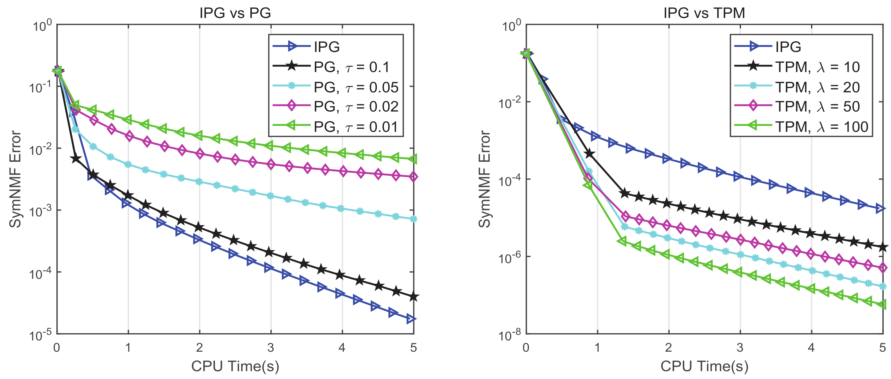
Compared with the classical PG method, IPG performs better. To see this, we generated 20 synthetic symmetric non-negative matrices and tested IPG and PG on them. Each of the generated matrices $A=H{H}^T$ was constructed using a random non-negative factor $H\in {\mathbb{R}}^{200\times 50}$, where the entries of H were uniformly distributed in $[0,1]$. We set ${\tau }_1=0.01$ and ${\tau }_2=0.1$ for IPG, and selected $\tau =0.01,0.02,0.05,0.1$ for PG. The left subgraph of Figure 1 shows the average SymNMF error

$$E\left(H\right)=\frac{\parallel A-H{H}^T{\parallel }_F}{{\parallel A\parallel }_F}$$

of each algorithm over the CPU time. The efficiency of IPG was always higher than that of PG, regardless of the parameters of PG.

2.3. The Two-Phase Method for Robust SymNMF

Combining Algorithms 1 and 2, we propose our two-phase method (TPM) for SymNMF. Each of these two phases has a unique effect on obtaining a stable SymNMF. The first phase alleviates the non-convexity of the problem by discarding the non-negativity constraints. Meanwhile, in this phase, we designed an NCG algorithm to quickly obtain a symmetric non-negative approximation of A. Although the convergence point of the first phase is not a stationary point of (2), it can be used as a good initial point for the second phase. In the second phase, we proposed the IPG algorithm, which continues to reduce the SymNMF error and converge to the stationary point of (2) very fast. The combination of these two phases enables us to efficiently solve the SymNMF problem. We summarize the whole procedure of TPM in Algorithm 3.

We also compared TPM with IPG on the synthetic symmetric non-negative matrices generated above. We selected $\mathsf{\lambda }=10,20,50,100$ for TPM. The right subgraph of Figure 1 shows the SymNMF error of each algorithm over the CPU time. The efficiency of TPM was always higher than that of IPG, regardless of the parameters of TPM.

Algorithm 3 Two-Phase Method (TPM) for SymNMF.

Require:  initial point H; parameters $\mathsf{\lambda }$, $0<\rho <\sigma <1$, $\mu \in (0,1)$, $\nu =0.1$, $0<{\tau }_1<{\tau }_2<1$, ${ϵ}_1>0$, ${ϵ}_2>0$; and maximum number of iterations for each phase $k_{max}^{\left(1\right)}$, $k_{max}^{\left(2\right)}$. Ensure:  a SymNMF factor of A: $H^{**}$. 1: Starting with H, run Algorithm 1 until $\parallel \nabla f\left(H_k\right){\parallel }_{\infty }<{ϵ}_1$ or the number of iterations exceeds $k_{\max }^{\left(1\right)}$. Denote the last $H_k$ obtained by Algorithm 1 as $H^{*}$. 2: Set $H_{+}^{*}=max\{H^{*},0\}$. 3: Starting with $H_{+}^{*}$, run Algorithm 2 until $\parallel H_k-{[H_k-(H_k{H}_k^T-A)H_k]}_{+}{\parallel }_{\infty }<{ϵ}_2$ or the number of iterations exceeds $k_{\max }^{\left(2\right)}$. Denote the last $H_k$ obtained by Algorithm 2 as $H^{**}$.

3. Numerical Experiments and Comparisons

In this section, we report the numerical performance of our method on both synthetic data and real-world data, compared to five state-of-the-art SymNMF approaches. The algorithms used for comparison included alternating non-negative least squares (ANLS) [14], block coordinate descent (BCD) [22], inexact block coordinate descent (IBCD) [23], hierarchical alternating non-negative least squares (HALS) [24], and accelerated multiplicative update (AMU) algorithms [20]. For synthetic data sets, we were concerned about the decline of the objective function and the convergence behavior near the stationary point. For real-world data sets, besides the above measurements, we focused on the clustering performance, in terms of accuracy and stability.

For ANLS, BCD, IBCD, and HALS, we used the respective MATLAB code provided by the authors. For AMU, we wrote the code ourselves and adopted the default setting for the parameters recommended by the authors. The parameter $\mathsf{\lambda }$ of TPM could be automatically set based on the sparsity of the matrix to be decomposed. Generally, one can set $\mathsf{\lambda }$ as

$$\begin{array}{c}\hfill \mathsf{\lambda }\approx \frac{10nnz}{n^2},\end{array}$$

(22)

where $nnz$ is the number of non-zeros entries in the matrix. In our experiments, according to (22), we simply set $\mathsf{\lambda }=10$ for synthetic examples (dense matrices) and $\mathsf{\lambda }=0.01$ for real-world data sets (sparse matrices). We implemented all the experiments in MATLAB 2020b on a Windows system using a PC with a 1.60 GHz Intel Core i5-8250U CPU and 8 GB of RAM.

3.1. Synthetic Data

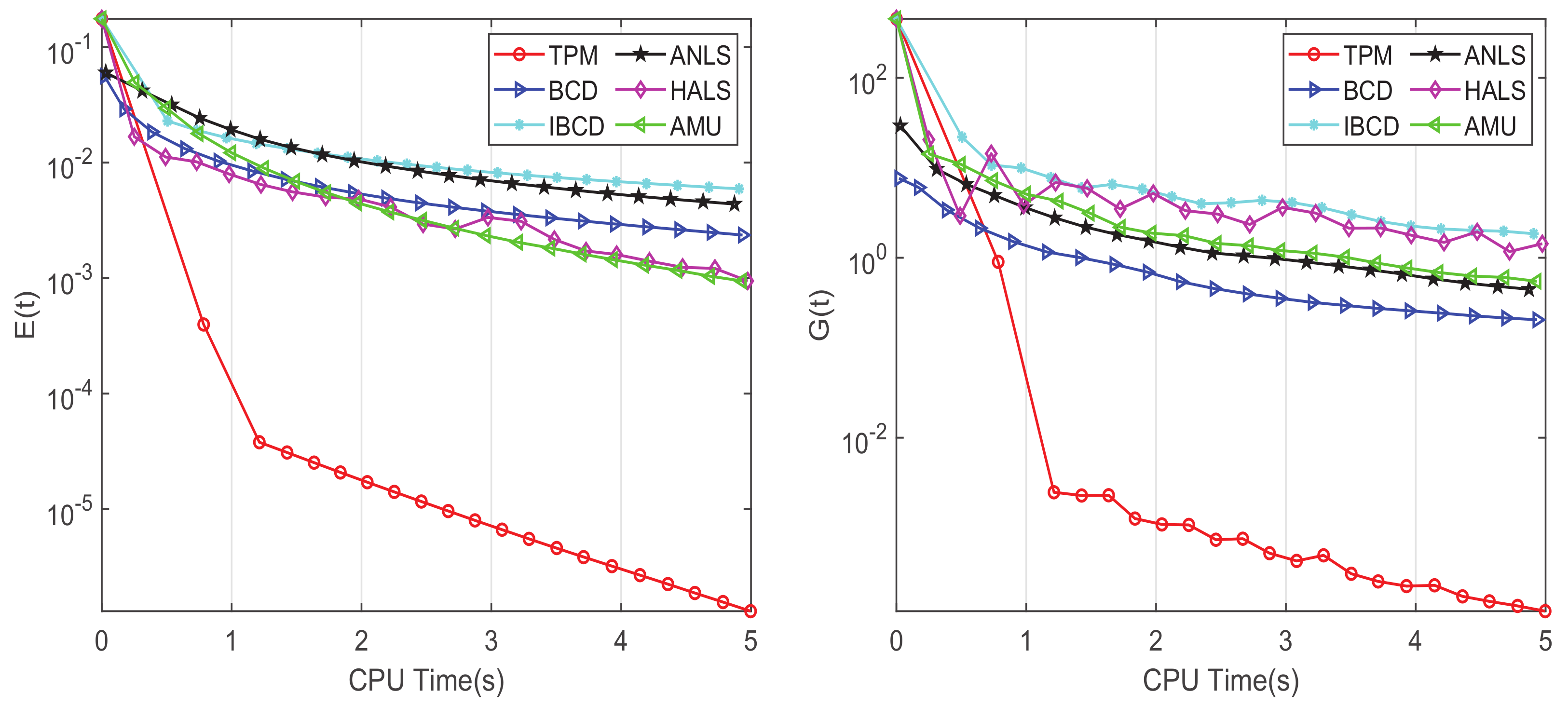
For the synthetic data sets, as in Section 2.2, we generated 20 symmetric non-negative matrices $A=H{H}^T$ by randomly constructing a non-negative factor $H\in {\mathbb{R}}^{n\times r}$ , where $n=200$, $r=50$, and the entries of H are uniformly distributed in $[0,1]$. Note that A is a completely positive matrix [32]; that is, A has an exact SymNMF.

To comprehensively evaluate the various algorithms, we adopted two criteria for the performance of SymNMF. The first one was the SymNMF error:

$$\begin{array}{c}\hfill \mathrm{E}\left(t\right)=\frac{{\parallel A-H\left(t\right)H\left(t\right)}^T{\parallel }_F}{{\parallel A\parallel }_F},\end{array}$$

(23)

where $H\left(t\right)$ represents the factor H achieved by an algorithm for a given initialization within t seconds. The other criterion was the optimal gap:

$$\begin{array}{c}\hfill \mathrm{G}\left(t\right)=\parallel H\left(t\right)-{[H(t)-(H(t)H{(t)}^T-A)H(t)]}_{+}{\parallel }_{\infty }\end{array}$$

(24)

mentioned in Section 2.2. Recall that $\mathrm{G}\left(t\right)$ is equal to zero if and only if $H\left(t\right)$ is a stationary point of (2). For each matrix, we executed all algorithms 10 times with different initial points, and stopped them when their elapsed time exceeded 5 s. The initial point was randomly generated in the form of ${\kappa }^{*}{H}_0$ [22], where $H_0$ is uniformly distributed in $[0,1]$ and ${\kappa }^{*}$ satisfies

$$\begin{array}{c}\hfill {\kappa }^{*}=arg\underset{\kappa >0}{min}{\parallel A-\left(\kappa H_0\right){\left(\kappa H_0\right)}^T\parallel }_F=\sqrt{\frac{\langle A{H}_0,H_0\rangle }{\parallel H_0^T{H}_0{\parallel }_F^2}}.\end{array}$$

(25)

Figure 2 shows the average E$\left(t\right)$ and G$\left(t\right)$ over 200 trials for each algorithm. We observed the following:

• The efficiency of TPM was much better than that of all other algorithms. This advantage was not only reflected in the decrease in the SymNMF error, but also in the speed at which the iteration approached a stationary point.
• TPM was capable to obtain SymNMF with better quality, compared to other algorithms. The average SymNMF error of TPM was less than ${10}^{-5}$, while the best result of the other SymNMF algorithms could only achieve an average SymNMF error of about ${10}^{-3}$.

The above observations demonstrate that TPM not only converged faster than other approaches but also could obtain SymNMF with lower error.

3.2. Real-World Data

In this subsection, we evaluated the performance of TPM and other SymNMF algorithms in real-world data sets from three perspectives: the SymNMF error, the clustering accuracy, and the stability. Given the affinity matrix $A\in {\mathbb{R}}^{n\times n}$ of a data set $\{x_1,\dots ,x_n\}$, SymNMF searched for a non-negative factor $H\in {\mathbb{R}}^{n\times r}$ satisfying $A\approx H{H}^T$, where r is the number of classes in the data set. The label of H was determined by the position of the largest component of each row of H; that is,

$$\ell \left(x_i\right)=arg\underset{j}{max}\{h_{i1},...,h_{ij},...,h_{ir}\}.$$

where $h_{ij}(1\le i\le n,1\le j\le r)$ is the entry of the i-th row and j-th column of H.

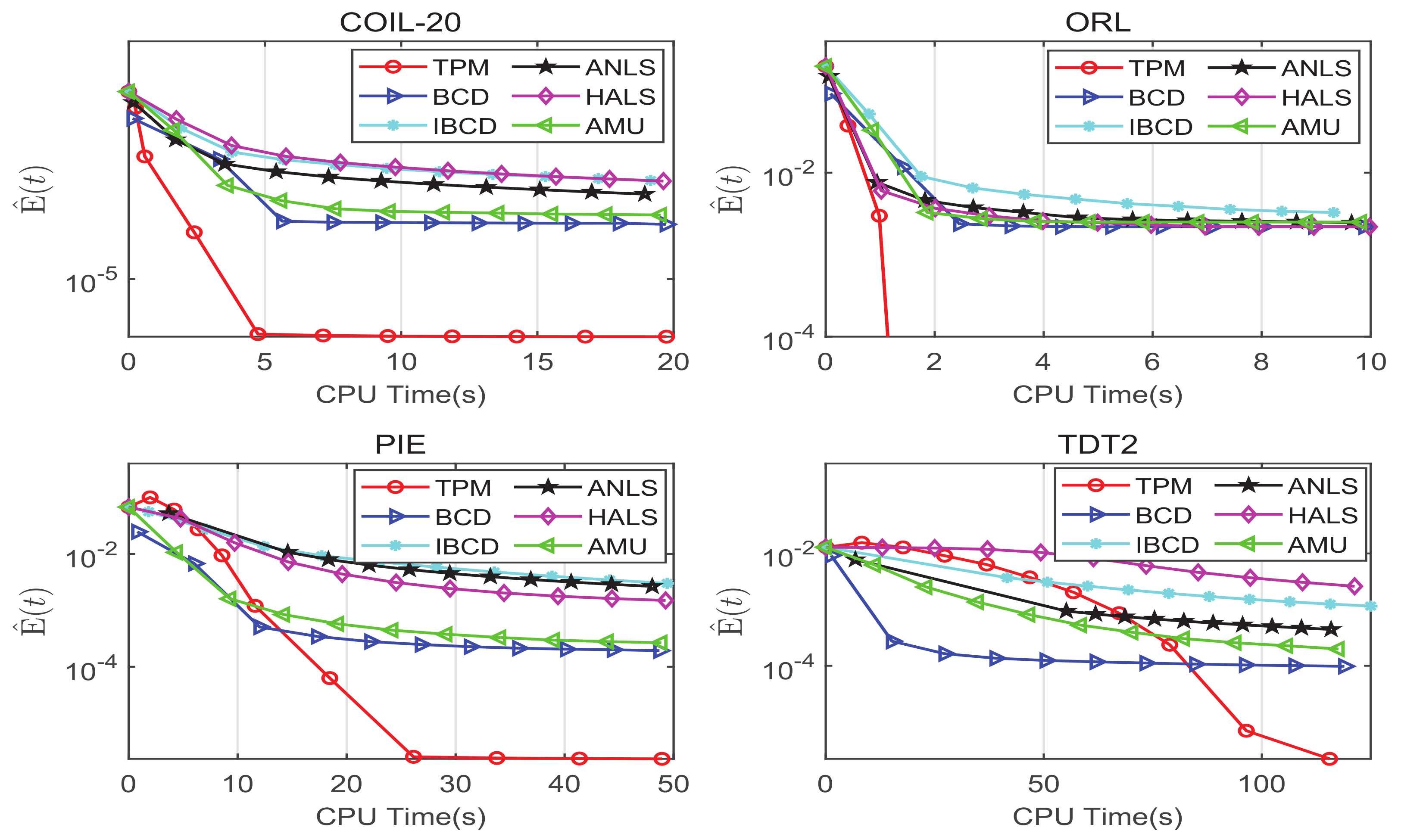
We conducted experiments on four data sets: COIL-20 [33] (https://www.cs.columbia.edu/CAVE/software/softlib/coil-20.php, accessed on 29 March 2021), ORL [34] (http://www.cl.cam.ac.uk/research/dtg/attarchive/facedatabase.html, accessed on 19 April 2021), PIE [35] (http://www.ri.cmu.edu/research_project_detail.html?project_id=418&menu_id=261, accessed on 27 April 2021), and TDT2 [36] (https://www.ldc.upenn.edu/collaborations/past-projects, accessed on 7 May 2021). Detailed information of these data sets is given in

Table 1. Data sets used in our experiments.

Data Name	Type	Dimension	# Data Points	# Clusters
COIL-20	object	32 × 32	1440	20
ORL	face	$92\times 112$	400	40
PIE	face	$32\times 32$	2856	68
TDT2	document	36,771	8741	20

.

The affinity matrix for each data set was constructed following the procedures given in [14]; that is,

• For the image data sets COIL-20, ORL, and PIE, we defined:

  $$e_{ij}=\left\{\begin{array}{cc}exp(-{\displaystyle \frac{\parallel x_i-x_j{\parallel }_2^2}{{\sigma }_i{\sigma }_j}}),\hfill & i\in {\mathcal{N}}_k\left(j\right)\mathrm{or}j\in {\mathcal{N}}_k\left(i\right);\hfill \\ 0,\hfill & \mathrm{otherwise},\hfill \end{array}\right.$$

  where ${\mathcal{N}}_k\left(i\right)$ is the set of k-nearest neighbors of $x_i$, and ${\sigma }_i$ is the Euclidean distance between $x_i$ and its $\widehat{k}$-th neighbor. We adopted $\widehat{k}=7$, as suggested in [37]. The affinity between $x_i$ and $x_j$ was defined by

  $$\begin{array}{c}\hfill a_{ij}=d_i^{1/2}{e}_{ij}{d}_j^{1/2},\end{array}$$

  (26)

  where $d_i={\sum }_{s=1}^n{e}_{is}$.
• For the document data set TDT2, all the document vectors $x_i$ were normalized to have unit 2-norm, and we defined:

  $$e_{ij}=\left\{\begin{array}{cc}{x}_i^T{x}_j,\hfill & i\in {\mathcal{N}}_k\left(j\right)\mathrm{or}j\in {\mathcal{N}}_k\left(i\right);\hfill \\ 0,\hfill & \mathrm{otherwise}.\hfill \end{array}\right.$$
  The affinity between $x_i$ and $x_j$ was also defined as in (26).

The parameter k in ${\mathcal{N}}_k\left(i\right)$ determined the sparseness of the affinity matrix. unlike the recommended $k=\left[{log}_2\left(n\right)\right]+1$ in [38] , we set k as $\left[{log}_2\left(\frac{n}{n_c}\right)\right]+1$, where $n_c$ is the class number of the data set. Compared with the original setting, our k was smaller, and the connected data points were more likely to be class consistent.

We executed all algorithms 20 times with different randomly constructed initial points, and stopped them when their elapsed time exceeds the time limit. For COIL-20, ORL, PIE, and TDT2, according to their sizes, the time limits were set as 20, 10, 50, and 120 s, respectively. To compare the average performance of the different algorithms, we denoted

$$\widehat{\mathrm{E}}\left(t\right)=\mathrm{E}\left(t\right)-E_{\min },$$

where $\mathrm{E}\left(t\right)$ is defined as in (23) and $E_{\min }$ is the smallest error obtained by all algorithms over all initializations. Figure 3 displays the average $\widehat{\mathrm{E}}\left(t\right)$ for each algorithm. In all cases, TPM performed best and can generate the solution with the lowest SymNMF error among all of the algorithms.

Besides the SymNMF error, we also compared the clustering performance for each algorithm. We adopted two criteria—average correction (AC) and normalized mutual information (NMI) [39]—to measure the clustering performance. The average values over all the 20 trials are listed in

Table 2. Clustering performance measured by AC (%) and NMI (%) on real-world databases.

Metric	Data Set	TPM	ANLS	BCD	IBCD	HALS	AMU
AC	COIL-20	82.98	74.52	60.25	65.77	56.16	71.04
	ORL	78.00	74.57	72.55	74.91	74.30	74.29
	PIE	86.91	80.04	48.32	50.27	56.61	78.80
	TDT2	93.30	87.15	56.31	69.57	33.59	79.93
NMI	COIL-20	91.63	88.13	78.75	81.00	73.22	86.61
	ORL	90.20	89.01	87.82	88.80	88.67	88.77
	PIE	94.96	93.11	76.56	77.53	81.26	92.55
	TDT2	88.33	85.81	62.18	70.53	34.69	80.92

. We observed that TPM performed better than the other algorithms. On COIL-20, ORL, PIE, and TDT2, we increased the highest clustering accuracy of existing methods by 8.46%, 3.09%, 6.87%, and 6.15% respectively. In order to further illustrate the clustering stability of all algorithms, we drew the results of 20 runs from different starting points in a box plot, as shown in Figure 4. Unlike the larger variance of other algorithms, the clustering results of TPM were very concentrated. This phenomenon demonstrated that TPM was very robust to the initial point.

4. Conclusions

In this paper, we proposed a two-phase algorithm for SymNMF. Our method is more efficient and robust than state-of-the-art algorithms, and performed well in real-world clustering tasks. Moreover, our algorithm is guaranteed to converge to the stationary solutions of the SymNMF problem. However, there are still some issues that need to be explored. First, although our algorithm has high efficiency, a theoretical analysis of the convergence rate should be conducted. Second, in real-world clustering tasks, the structure of the graph can significantly affect the clustering results obtained by the SymNMF algorithm. Thirdly, we need to consider how to reduce the time complexity and the storage requirements of the algorithm when processing large-scale data. The distributed-memory parallel strategy proposed in [40] provides a good inspiration. In the future, we intend to carry out further research on the above-mentioned issues.

References

- Lee, D.D.; Seung, H.S. Learning the parts of objects by non-negative matrix factorization. Nature 1999, 401, 788–791. [Google Scholar] [CrossRef] [PubMed]
- Liu, W.; Zheng, N. Non-negative matrix factorization based methods for object recognition. Pattern Recognit. Lett. 2004, 25, 893–897. [Google Scholar] [CrossRef]
- David, G.; Jordi, V. Non-negative Matrix Factorization for Face Recognition. In Proceedings of the 5th Catalonian Conference on AI: Topics in Artificial Intelligence, Castellón, Spain, 24–25 October 2002; pp. 336–344. [Google Scholar]
- Zdunek, R.; Cichocki, A. Non-negative Matrix Factorization with Quasi-Newton Optimization. In Proceedings of the Artificial Intelligence and Soft Computing, Zakopane, Poland, 25–29 June 2006; pp. 870–879. [Google Scholar]
- Jose, M.B.D.; Plaza, A.; Dobigeon, N.; Parente, M.; Du, Q.; Gader, P.; Chanussot, J. Hyperspectral Unmixing Overview: Geometrical, Statistical, and Sparse Regression-Based Approaches. IEEE J. Sel. Top. Appl. Earth Obs. Remote Sens. 2012, 5, 354–379. [Google Scholar]
- Hoyer, P.O. Non-Negative Matrix Factorization with Sparseness Constraints. J. Mach. Learn. Res. 2004, 5, 1457–1469. [Google Scholar]
- Ding, C.; Li, T.; Peng, W.; Park, H. Orthogonal nonnegative matrix t-factorizations for clustering. In Proceedings of the 12th ACM SIGKDD International Conference on Knowledge Discovery and Data Mining, Philadelphia, PA, USA, 20–23 August 2006; pp. 126–135. [Google Scholar]
- Cai, D.; He, X.; Han, J.; Huang, T.S. Graph Regularized Nonnegative Matrix Factorization for Data Representation. IEEE Trans. Pattern Anal. Mach. Intell. 2011, 33, 1548–1560. [Google Scholar]
- Wang, Y.; Zhang, Y. Nonnegative Matrix Factorization: A Comprehensive Review. IEEE Trans. Knowl. Data Eng. 2013, 25, 1336–1353. [Google Scholar] [CrossRef]
- Esposito, F. A Review on Initialization Methods for Nonnegative Matrix Factorization: Towards Omics Data Experiments. Mathematics 2021, 9, 1006. [Google Scholar] [CrossRef]
- Yang, M.S. A survey of fuzzy clustering. Math. Comput. Model. 1993, 18, 1–16. [Google Scholar] [CrossRef]
- Zass, R.; Shashua, A. A unifying approach to hard and probabilistic clustering. In Proceedings of the IEEE International Conference on Computer Vision, Beijing, China, 17–21 October 2005; pp. 294–301. [Google Scholar]
- Raviteja, V.; Kim, Ø.R.; Gopinath, C.; Boian, A. Determination of the number of clusters by symmetric non-negative matrix factorization. In Proceedings of the Big Data III: Learning, Analytics, and Applications, Online, 12 April 2021; Volume 11730, p. 15. [Google Scholar]
- Kuang, D.; Yun, S.; Park, H. SymNMF: Nonnegative low-rank approximation of a similarity matrix for graph clustering. J. Glob. Optim. 2015, 62, 545–574. [Google Scholar] [CrossRef]
- Ma, Y.; Hu, X.; He, T.; Jiang, X. Hessian Regularization Based Symmetric Nonnegative Matrix Factorization for Clustering Gene Expression and Microbiome Data. Methods 2016, 111, 80–84. [Google Scholar] [CrossRef]
- Lloyd, S.P. Least squares quantization in PCM. IEEE Trans. Inf. Theory 1982, 28, 129–137. [Google Scholar] [CrossRef]
- Jolliffe, I.T. Principal Component Analysis. J. Mark. Res. 2002, 87, 513. [Google Scholar]
- Ng, A.Y.; Jordan, M.I.; Weiss, Y. On Spectral Clustering: Analysis and an Algorithm. In Proceedings of the Advances in Neural Information Processing Systems, Vancouver, BC, Canada, 14 April 2001; pp. 849–856. [Google Scholar]
- He, Z.; Xie, S.; Zdunek, R.; Zhou, G.; Cichocki, A. Symmetric Nonnegative Matrix Factorization: Algorithms and Applications to Probabilistic Clustering. IEEE Trans. Neural Netw. 2011, 22, 2117–2131. [Google Scholar]
- Wang, P.; He, Z.; Lu, J.; Tan, B.; Bai, Y.; Tan, J.; Liu, T.; Lin, Z. An Accelerated Symmetric Nonnegative Matrix Factorization Algorithm Using Extrapolation. Symmetry 2020, 12, 1187. [Google Scholar] [CrossRef]
- Wright, S.J. Coordinate Descent Algorithms. Math. Program. 2015, 151, 3–34. [Google Scholar] [CrossRef]
- Vandaele, A.; Gillis, N.; Lei, Q.; Zhong, K.; Dhillon, I. Efficient and Non-Convex Coordinate Descent for Symmetric Nonnegative Matrix Factorization. IEEE Trans. Signal Process. 2016, 64, 5571–5584. [Google Scholar] [CrossRef]
- Shi, Q.; Sun, H.; Lu, S.; Hong, M.; Razaviyayn, M. Inexact Block Coordinate Descent Methods for Symmetric Nonnegative Matrix Factorization. IEEE Trans. Signal Process. 2017, 65, 5995–6008. [Google Scholar] [CrossRef] [Green Version]
- Zhu, Z.; Li, X.; Liu, K.; Li, Q. Dropping Symmetry for Fast Symmetric Nonnegative Matrix Factorization. arXiv 2018, arXiv:1811.05642. [Google Scholar]
- Polyak, B.T. The conjugate gradient method in extremal problems. USSR Comput. Math. Math. Phys. 1969, 9, 94–112. [Google Scholar] [CrossRef]
- Nocedal, J.; Wright, S. Numerical Optimization; Springer Science & Business Media: New York, NY, USA, 2006. [Google Scholar]
- Zhang, Z.; Li, B. Exterior Point Method for Completely Positive Factorization. arXiv 2021, arXiv:2102.08048. [Google Scholar]
- Sun, W.; Yuan, Y. Optimization Theory and Methods: Nonlinear Programming; Springer Science & Business Media: New York, NY, USA, 2006. [Google Scholar]
- Kuang, D.; Ding, C.; Park, H. Symmetric Nonnegative Matrix Factorization for Graph Clustering. In Proceedings of the 2012 SIAM International Conference on Data Mining (SDM), Anaheim, CA, USA, 26–28 April 2012; pp. 106–117. [Google Scholar]
- Calamai, P.; More, J. Projected gradient methods for linearly constrained problems. Math. Program. 1987, 39, 93–116. [Google Scholar] [CrossRef]
- Razaviyayn, M.; Hong, M.; Luo, Z.Q.; Pang, J.S. Parallel Successive Convex Approximation for Nonsmooth Nonconvex Optimization. In Proceedings of the Advances in Neural Information Processing Systems, Montreal, QC, Canada, 8–13 December 2014; pp. 1440–1448. [Google Scholar]
- Shaked-Monderer, N.; Berman, A. Copositive and Completely Positive Matrices; World Scienfic: Hackensack, NJ, USA, 2021. [Google Scholar]
- Nene, S.; Nayar, S.; Murase, H. Columbia Object Image Library (COIL-20); Tech. Rep. CUCS-005-96; Columbia University: New York, NY, USA, 1996. [Google Scholar]
- Samaria, F.; Harter, A. Parameterisation of a stochastic model for human face identification. In Proceedings of the Second IEEE Workshop on Applications of Computer Vision, Sarasota, FL, USA, 5–7 December 1994; pp. 138–142. [Google Scholar]
- Sim, T.; Baker, S.; Bsat, M. The CMU Pose, Illumination, and Expression (PIE) database. In Proceedings of the Fifth IEEE International Conference on Automatic Face Gesture Recognition, Washinton, DC, USA, 20–21 May 2002; pp. 46–51. [Google Scholar]
- Fiscus, J.; Doddington, G.; Garofolo, J.; Alvin, M. NIST’s 1998 Topic Detection and Tracking evaluation (TDT2). In Proceedings of the 1999 DARPA Broadcast News Workshop, Herndon, VA, USA, 28 February–3 March 1999; pp. 19–24. [Google Scholar]
- Zelnik-Manor, L.; Perona, P. Self-Tuning Spectral Clustering. In Proceedings of the Advances in Neural Information Processing Systems, Vancouver, BC, Canada, 13–18 December 2004; pp. 1601–1608. [Google Scholar]
- Luxburg, U.V. A Tutorial on Spectral Clustering. Stat. Comput. 2004, 17, 395–416. [Google Scholar] [CrossRef]
- Wu, W.; Jia, Y.; Kwong, S.; Hou, J. Pairwise Constraint Propagation-Induced Symmetric Nonnegative Matrix Factorization. IEEE Trans. Neural Netw. Learn. Syst. 2018, 29, 6348–6361. [Google Scholar] [CrossRef]
- Eswar, S.; Hayashi, K.; Ballard, G.; Kannan, R.; Vuduc, R.; Park, H. Distributed-Memory Parallel Symmetric Nonnegative Matrix Factorization. In Proceedings of the SC20: The International Conference for High Performance Computing, Networking, Storage and Analysis, Atlanta, GA, USA, 9–19 November 2020; pp. 1–14. [Google Scholar]
Figure 1.
The average SymNMF error versus run–time on the synthetic data.
Figure 2.
The average and (from left to right) of six SymNMF algorithms versus run–time on the synthetic data.
Figure 3.
The average of six SymNMF algorithms versus run–time on real–world data sets.
Figure 4.
Box-plot of the clustering results of six algorithms on four real-world data sets.