Numerical Modelling of Multicellular Spheroid Compression: Viscoelastic Fluid vs. Viscoelastic Solid

Abstract

Parallel-plate compression of multicellular spheroids (MCSs) is a promising and popular technique to quantify the viscoelastic properties of living tissues. This work presents two different approaches to the simulation of the MCS compression based on viscoelastic solid and viscoelastic fluid models. The first one is the standard linear solid model implemented in ABAQUS/CAE. The second one is the new model for 3D viscoelastic free surface fluid flow, which combines the Oldroyd-B incompressible fluid model and the incompressible neo-Hookean solid model via incorporation of an additional elastic tensor and a dynamic equation for it. The simulation results indicate that either approach can be applied to model the MCS compression with reasonable accuracy. Future application of the viscoelastic free surface fluid model is the MCSs fusion highly-demanded in bioprinting.

1. Introduction

Mechanical properties of cells, cellular substrates, and biological tissues have been demonstrated to play a crucial role in many physiological and pathological processes [1,2]. The mechanical behavior of soft biological objects is time-dependent and combines both solid- and liquid-like aspects [3,4,5]. Therefore, it is often investigated using analogies with inert soft condensed matter, either liquid or solids, including such models as viscoelastic solids, pastes, foams, and liquids with surface tension [6]. Multicellular spheroids (MCSs), three-dimensional spherical cellular aggregates, are part of a good in vitro model system to explore tissue biomechanics [7]. The biological and mechanical properties of MCS result from the complex interactions of its constituents, which are cells, extracellular matrix, liquid medium, and that include intracellular adhesion, active force and tension generation by cells, liquid diffusion, and cell and matrix rearrangements [7].

Even though a large number of mechanical models currently exist, none of them can fully account for all components and describe a full reach spectrum of MCS mechanical behavior, which can be observed during a time-dependent response to compression, shape changes after the incision, and the fusion of two or more MCSs. Even though the creation of an ideal model does not seem feasible at the moment, the models that can describe particular aspects should be developed, tested, and compared. From the practical perspective, knowledge of the biomechanical properties of cellular aggregates will improve the quality of the tissue engineering constructs. Cell aggregates hold the potential to be widely utilized as building blocks for the construction of complex tissues via fusion and bioprinting [8].

We address viscoelasticity-based simulations of an experiment on parallel-plate compression [9] of spheroids generated from mesenchymal stromal cells. Viscoelastic phenomena have been taken into account in solid deformation models of the parallel-plate MCS compression in the literature (see [10,11] and references therein). For the simulation of viscoelastic solid deformations we exploit the finite element ABAQUS/CAE software, which is based on the model of linear isotropic viscoelasticity [12]. Although 3D viscoelastic fluid models have been used in many applications [13,14,15], to the best of our knowledge only 1D viscoelastic fluid flow models were applied to cells and multicellular aggregates mechanics problems such as compression tests (we refer for a review to Table 1 from [10]). In this paper, we suggest a new 3D viscoelastic free surface fluid flow model of the parallel-plate MCS compression and compare it with the 3D linear isotropic viscoelastic solid deformation model.

The description of viscoelastic fluid flows is based on differential constitutive equations such as Upper-Convected Maxwell (UCM) [16], Oldroyd-B [17], Giesekus [18], Phan–Thien–Tanner [19] and others, as well as on integral constitutive equations [20,21]. Due to its relative simplicity, the differential form of the UCM and Oldroyd-B models laid the foundation for the benchmarking of numerical models [14,15,22,23]. The simulations of flows of UCM and Oldroyd-B free surface fluids are based on finite elements [24,25], finite volumes [13], smoothed particle hydrodynamics [26,27,28], finite differences on staggered MAC grids [14,29,30], the lattice Boltzmann method [31] and so forth. Numerical treatment of the free surface tracking is provided by the volume of fluid (VOF) method [32], the front tracking by massless markers [33], or the front capturing by the level set method [34]. We exploit the level set method, which represents the free surface by the zero isolevel of a globally defined level set function advected by the fluid velocity field, since it allows us to process complex topological changes on the surface. Although this feature is not used in the simulation of the parallel-plate MCS compression, it is important for other experiments such as the fusion of MCSs.

The novelty of our paper is the new model for 3D viscoelastic free surface fluid flow applicable to the parallel-plate MCS compression experiment. The model combines the Oldroyd-B incompressible fluid model and the neo-Hookean incompressible solid model via the incorporation of an additional elastic tensor and a dynamic equation for it. The numerical model of the Oldroyd-B incompressible free surface fluid is discussed in [35]. The neo-Hookean model is one of the hyperelastic material models, which are widely used for the evaluation of the mechanical properties of single cells [3,36,37]. It is known to be reasonably accurate for incompressible soft tissues undergoing strains of up to 100% [38,39]. The second important contribution of the present paper is direct comparison of the simulated and experimental data for the MCS compression.

The rest of the paper is organized as follows. In Section 2 we present the 3D models for isotropic viscoelastic solid deformation and viscoelastic free surface fluid flow. In Section 3 we discuss the numerical results and compare them with experimental data for the parallel-plate MCS compression.

2. Materials and Methods

In this section, we discuss viscoelastic models of solid and fluid which are applicable to the description of the MCS compression and describe the protocol of the experiment.

2.1. Viscoelastic Solid Model

Since the compression of a multicellular spheroid is assumed to be slow enough, the inertia forces can be neglected and the deformation can be described by a sequence of quasi-static states of a linear isotropic viscoelastic solid. Each quasi-static state of a body with current volume V and surface S is governed by the virtual work principle:

$$\begin{array}{c}\hfill \underset{V}{\int }\mathit{\sigma }:\delta \mathbf{D}dV=\underset{S}{\int }\mathbf{t}·\delta \mathbf{v}dS+\underset{V}{\int }\mathbf{f}·\delta \mathbf{v}dV,\end{array}$$

(1)

where $\mathit{\sigma }$ is the total Cauchy stress, $\mathbf{D}=\frac{\nabla \mathbf{v}+{(\nabla \mathbf{v})}^T}{2}$ is the strain-rate tensor, $\mathbf{v}$ is the virtual velocity field, $\mathbf{t}=\mathbf{n}·\mathit{\sigma }$ is the traction vector, $\mathbf{f}$ is the external force. Contact and traction free boundary conditions complement the mechanical problem.

The constitutive law for the total stress of a linear isotropic viscoelastic material is time-dependent and is defined by the following integral equation in case of small deformations:

$$\begin{array}{c}\hfill \mathit{\sigma }\left(t\right)=\underset{0}{\overset{t}{\int }}2G(t-t^{{}^{\prime }})\dot{\mathbf{e}}d{t}^{{}^{\prime }}+\mathbf{I}\underset{0}{\overset{t}{\int }}K(t-t^{{}^{\prime }})\dot{\phi }d{t}^{{}^{\prime }},\end{array}$$

(2)

where $\mathbf{e}$ and $\phi$ are the mechanical deviatoric and volumetric strains; K is the bulk modulus and G is the shear modulus, $\dot{a}$ denotes differentiation of a with respect to $t^{{}^{\prime }}$. The generalization [12] of (2) to finite strains is:

$$\begin{array}{cc}\hfill \mathit{\sigma }\left(t\right)=2G\left(0\right)\mathbf{e}\left(t\right)+\mathrm{dev}& \left[\underset{0}{\overset{t}{\int }}{\mathbf{F}}_t^{-1}(t-t^{{}^{\prime }})\left(2\dot{G}\left(t^{{}^{\prime }}\right)\dot{\mathbf{e}}(t-t^{{}^{\prime }})\right){\mathbf{F}}_t(t-t^{{}^{\prime }})d{t}^{{}^{\prime }}\right]\hfill \\ \hfill +\mathbf{I}& \left(K\left(0\right)\phi \left(t\right)+\underset{0}{\overset{t}{\int }}\dot{K}\left(t^{{}^{\prime }}\right)\dot{\phi }(t-t^{{}^{\prime }})d{t}^{{}^{\prime }}\right),\hfill \end{array}$$

(3)

where $\mathrm{dev}\left[\mathbf{C}\right]:=\mathbf{C}-\frac{1}{3}\mathrm{tr}\left(\mathbf{C}\right)\mathbf{I}$ is the deviatoric part of a tensor $\mathbf{C}$, ${\mathbf{F}}_t(t-t^{{}^{\prime }})$ is the deformation gradient of the state at $t-t^{{}^{\prime }}$ relative to the state at t.

Viscoelasticity properties are controlled by Young modulus E and Poisson ratio $\nu$, the parameters of the standard linear solid model, and the time-dependent shear modulus $G\left(t\right)$:

$$\begin{array}{c}\hfill G\left(t\right)=G_{\infty }+(G_0-G_{\infty })e^{-t/{\lambda }_1},\end{array}$$

(4)

where ${\lambda }_1$ is the elastic relaxation time, $G_{\infty }=\underset{t\to \infty }{lim}G\left(t\right)$ and $G_0=G\left(0\right)=\frac{E}{2(1+\nu )}$ are the long-term and instantaneous shear moduli. The use of (4) implies setting two parameters $\alpha =\frac{G_{\infty }}{G_0}$ and ${\lambda }_1$. In order to compare the simulation results with the results produced by the incompressible viscoelastic fluid model, we neglect the compressibility of the solid by setting $\nu =0.5$, $\phi =0$ and discard the third term of (3).

The finite element implementation of the virtual work principle results in a sequence of nonlinear systems to be solved at each time step of the simulation based on the quasi-static process assumption.

2.2. Viscoelastic Fluid Model

The viscoelastic fluid model expands the Oldroyd-B fluid model by introducing an additional stress component described by the incompressible neo-Hookean constitutive law [40,41] as follows. The velocity $\mathbf{v}$ of incompressible non-Newtonian fluid in the gravity field satisfies the Navier–Stokes equations:

$$\begin{array}{cc}\hfill \rho \left(\frac{\partial \mathbf{v}}{\partial t}+(\mathbf{v}·\nabla )\mathbf{v}\right)& =-\nabla p+\nabla ·\mathit{\tau }+\rho \mathbf{g},\hfill \end{array}$$

(5)

$$\begin{array}{cc}\hfill \nabla ·\mathbf{v}& =0,\hfill \end{array}$$

(6)

with the initial condition at the state of rest and appropriate boundary conditions.

The fluid stress tensor $\mathit{\tau }$ is split into two parts. The first part is governed by the Oldroyd-B fluid model [17], the second one is governed by the incompressible neo-Hookean model of hyperelastic solid [40,41]:

$$\begin{array}{cc}\hfill \mathit{\tau }& ={\mathit{\tau }}_1+{\mathit{\tau }}_2,\hfill \end{array}$$

(7)

$$\begin{array}{cc}\hfill {\mathit{\tau }}_1+{\lambda }_1{\stackrel{▿}{\mathit{\tau }}}_1& =2(1-\alpha ){\lambda }_1{G}_0(\mathbf{D}+{\lambda }_2\stackrel{▿}{\mathbf{D}}),\hfill \end{array}$$

(8)

$$\begin{array}{cc}\hfill {\stackrel{▿}{\mathit{\tau }}}_2& =2\alpha G_0\mathbf{D},\hfill \end{array}$$

(9)

where $\mathbf{D}=\frac{\nabla \mathbf{v}+{(\nabla \mathbf{v})}^T}{2}$ is the strain-rate tensor, parameters $G_0$, ${\lambda }_1$ and $\alpha <1$ define the shear modulus (4), ${\lambda }_2=\beta {\lambda }_1$, $\beta <1$ is the retardation parameter, and $\stackrel{▿}{\mathbf{C}}$ denotes the first order upper-convected derivative for a tensor $\mathbf{C}$,

$$\stackrel{▿}{\mathbf{C}}=\frac{\partial \mathbf{C}}{\partial t}+\left(\mathbf{v}·\nabla \right)\mathbf{C}-{(\nabla \mathbf{v})}^T\mathbf{C}-\mathbf{C}(\nabla \mathbf{v}).$$

(10)

Note that by definition $\stackrel{▿}{\mathbf{I}}=-2\mathbf{D}$.

The next step is to express the constitutive Equations (7)–(9) in terms of the fluid stress tensor $\mathit{\tau }$. Summing (8) and (9) multiplied by ${\lambda }_1$ and eliminating ${\stackrel{▿}{\mathit{\tau }}}_1$ yields the following identity for $\mathit{\tau }$:

$$\begin{array}{c}\hfill \stackrel{▿}{\mathit{\tau }}-2{\lambda }_1{G}_0\stackrel{▿}{\mathbf{D}}+{\lambda }_1\stackrel{▿▿}{\mathit{\tau }}-2(1-\alpha ){\lambda }_1{\lambda }_2{G}_0\stackrel{▿▿}{\mathbf{D}}=2\alpha G_0\mathbf{D},\end{array}$$

(11)

where $\stackrel{▿▿}{\mathbf{C}}:=\stackrel{▿}{\stackrel{▿}{\mathbf{C}}}$.

In order to simplify (11), we perform the rheological splitting of the fluid stress tensor $\mathit{\tau }$ into viscous and elastic stress parts:

$$\begin{array}{cc}\hfill \mathit{\tau }& =2(1-\alpha )\beta {\lambda }_1{G}_0\mathbf{D}+{\mathit{\tau }}_P,\hfill \end{array}$$

(12)

$$\begin{array}{cc}\hfill {\stackrel{▿}{\mathit{\tau }}}_P& =2(1-(1-\alpha )\beta )G_0\mathbf{D}+{\mathbf{B}}_1,\hfill \end{array}$$

(13)

where ${\mathbf{B}}_1$ is the remaining elastic tensor part satisfying the equation

$$\begin{array}{c}\hfill {\mathbf{B}}_1+{\lambda }_1{\stackrel{▿}{\mathbf{B}}}_1=2(1-\alpha )(\beta -1)G_0\mathbf{D}.\end{array}$$

(14)

Substitution for ${\mathbf{B}}_1=\frac{(1-\alpha )(\beta -1)G_0}{{\lambda }_1}({\mathbf{A}}_1-\mathbf{I})$ reduces (14) to

$$\begin{array}{c}\hfill {\stackrel{▿}{\mathbf{A}}}_1=\frac{\mathbf{I}-{\mathbf{A}}_1}{{\lambda }_1}.\end{array}$$

(15)

Substitution for ${\mathit{\tau }}_P=(1-(1-\alpha )\beta )G_0({\mathbf{A}}_2-\mathbf{I})$ eliminates the strain-rate term in (13):

$$\begin{array}{c}\hfill {\stackrel{▿}{\mathbf{A}}}_2=\frac{{\mathbf{B}}_1}{(1-(1-\alpha )\beta )G_0}=\frac{(1-\alpha )(1-\beta )}{1-(1-\alpha )\beta }\frac{\mathbf{I}-{\mathbf{A}}_1}{{\lambda }_1}.\end{array}$$

(16)

Finally, the governing equations for the fluid stress tensor $\mathit{\tau }$ with unknown elastic tensors ${\mathbf{A}}_1$, ${\mathbf{A}}_2$ are written as follows:

$$\begin{array}{c}\hfill \mathit{\tau }=2(1-\alpha )\beta {\lambda }_1{G}_0\mathbf{D}+(1-(1-\alpha )\beta )G_0({\mathbf{A}}_2-\mathbf{I}),\end{array}$$

(17)

$$\begin{array}{c}\hfill {\stackrel{▿}{\mathbf{A}}}_2=\frac{(1-\alpha )(1-\beta )}{1-(1-\alpha )\beta }\frac{\mathbf{I}-{\mathbf{A}}_1}{{\lambda }_1},\end{array}$$

(18)

$$\begin{array}{c}\hfill {\stackrel{▿}{\mathbf{A}}}_1=\frac{\mathbf{I}-{\mathbf{A}}_1}{{\lambda }_1}.\end{array}$$

(19)

We assume that no elastic deformations are initially present, which leads to the conditions on the elastic tensors ${\mathbf{A}}_1{|}_{t=0}=\mathbf{I}$ and ${\mathbf{A}}_2{|}_{t=0}=\mathbf{I}$. Another assumption is that tensors ${\mathbf{A}}_1,{\mathbf{A}}_2$ possess the same boundary conditions: homogeneous Neumann at the contact boundary and zero traction at the free boundary [35].

Remark. For $\alpha =0$, the model (17)–(19) reduces to the standard Oldroyd-B fluid model with the conformation tensor ${\mathbf{A}}_1$

$$\begin{array}{c}\hfill \mathit{\tau }=2\beta {\lambda }_1{G}_0\mathbf{D}+(1-\beta )G_0({\mathbf{A}}_1-\mathbf{I}),\\ \hfill {\stackrel{▿}{\mathbf{A}}}_1=\frac{\mathbf{I}-{\mathbf{A}}_1}{{\lambda }_1}.\end{array}$$

Indeed, the Equations (18) and (19) possess the same right hand side $\frac{\mathbf{I}-{\mathbf{A}}_1}{{\lambda }_1}$; since tensors ${\mathbf{A}}_1,{\mathbf{A}}_2$ possess the same initial and boundary conditions, one derives ${\mathbf{A}}_1\left(t\right)={\mathbf{A}}_2\left(t\right)$.

Keeping in mind future applications of MCSs fusion, we address fluids with a free surface boundary. The boundary position $\mathsf{\Gamma }\left(t\right)$ is determined by the zero level isosurface of a globally defined level set function $\varphi (t,\mathbf{x})$ [34]:

$$\begin{array}{c}\hfill \varphi (t,\mathbf{x})\left\{\begin{array}{c}<0,\mathbf{x}\in \mathsf{\Omega }\left(t\right)\hfill \\ >0,\mathbf{x}\in {\mathbb{R}}^3\setminus \overline{\mathsf{\Omega }\left(t\right)}\hfill \\ =0,\mathbf{x}\in \mathsf{\Gamma }\left(t\right)\hfill \end{array}\right.\forall t\in [0,T].\end{array}$$

The level set function $\varphi$ satisfies the transport equation for $t>0$:

$$\begin{array}{c}\hfill \frac{\partial \varphi }{\partial t}+\tilde{\mathbf{v}}·\nabla \varphi =0\mathrm{in}{\mathbb{R}}^3\times (0,T],\end{array}$$

(20)

where the fluid velocity field $\mathbf{v}$ is extended outside $\mathsf{\Omega }\left(t\right)$ to get $\tilde{\mathbf{v}}$ in ${\mathbb{R}}^3$. Initially, the domain $\mathsf{\Omega }\left(0\right)$ is defined by $\{\mathbf{x},\varphi (0,\mathbf{x})<0\}$. For details of the level set function processing and the finite volume semi-implicit discretization of (5), (6), (17), (18), (19), (20) we refer to [35].

2.3. Measurements on Multicellular Spheroids

The multicellular spheroids were constructed from a primary human somatic cell culture of limbal mesenchymal stem cells (MSCs). Cells of the 4th passage were used. The technique for the spheroid preparation is described in detail in [42,43,44]. Briefly, MSCs were generated on agarose plates [45] prepared using a 3D Petri Dish (Microtissues, Providence, RI, USA). The spheroids formation occurred under standard conditions (37 ${}^{\circ }$C, 5% CO${}_2$) for seven days.

The parallel-plate compression was performed using a micro-scale testing system (Microsquisher, CellScale, Waterloo, ON, Canada) and associated SquisherJoy software. The experimental apparatus and protocol are described in detail in [46,47,48]. The spheroids were compressed between a fixed, rigid substrate and a displaceable cantilever beam with an attached flat platform in a PBS-filled bath. Compression of up to 50% of the initial spheroid height with a speed of 3 um/s was accompanied by simultaneous recording of the reaction force, the upper plate position, as well as the spheroid shape by the side-view camera.

The compression test consisted of three sequential phases. In the first phase (compress), within 36 s the upper plate moved towards the lower one with constant speed. In the second phase (hold), within 60 s the upper plate remained still. In the third phase (release), the upper plate moved away from the lower plate with the same constant speed as in the first phase. According to the experimental evidence, the multicellular spheroid regained partially its shape by the end of the release phase. Viscoelastic properties of the spheroid manifested themselves in all three phases.

3. Results and Discussion

3.1. Model Setting

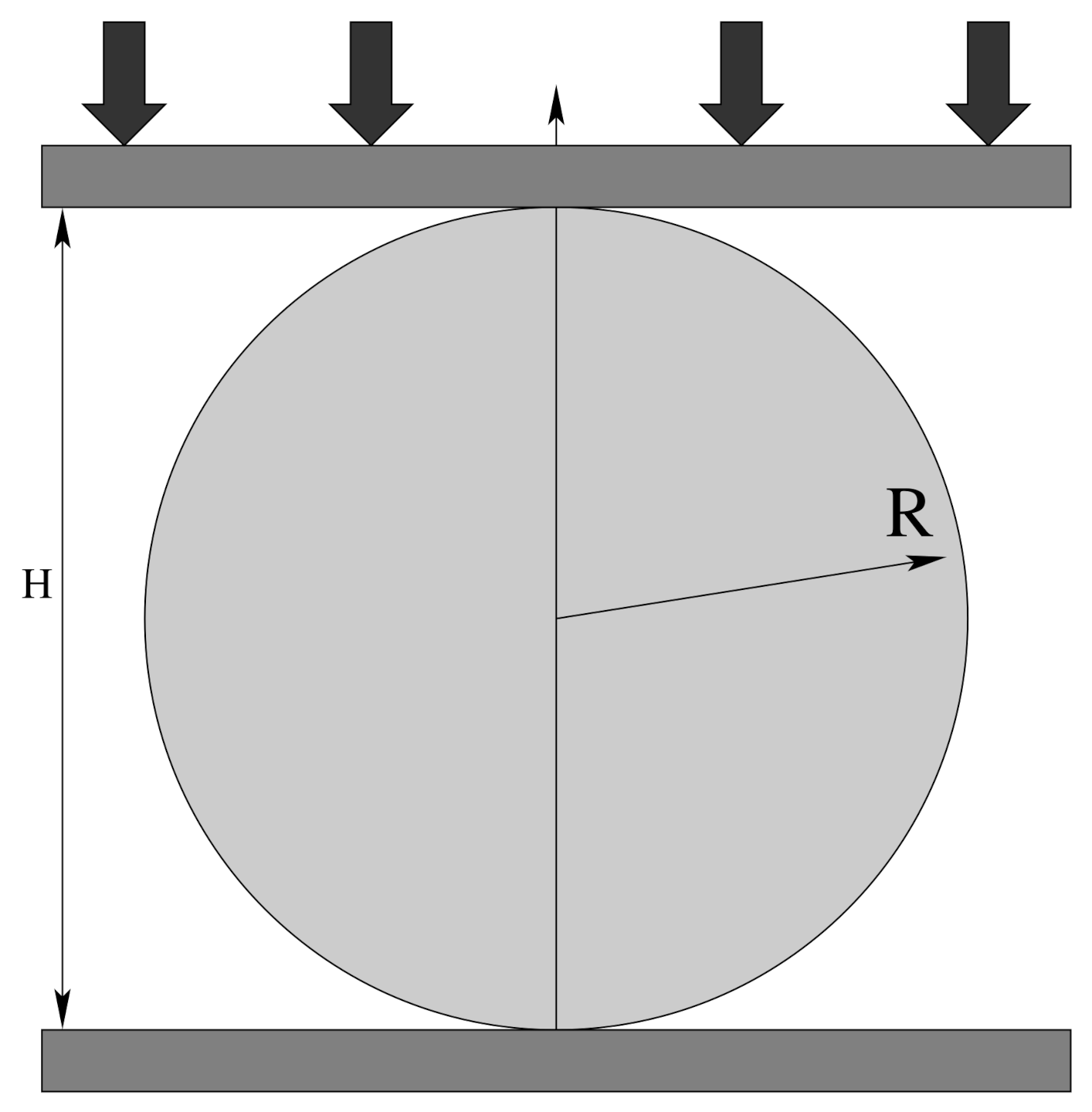
The experimental setup is shown schematically in Figure 1. The spheroid with radius $R=0.11\mathrm{mm}$ is located between the upper and lower plates touching both plates. The upper plate may move towards the lower plate and back.

During all three phases of the numerical test, one computes the distance H between the lower and upper points of the spheroid and the reaction force F acting on the upper plate. The force in both viscoelastic models is computed according to the definition of the reaction force:

$$\begin{array}{c}\hfill F=\underset{S}{\int }\mathbf{n}·\overline{\mathit{\sigma }}\mathbf{n}dS,\end{array}$$

(21)

where S is the contact surface, $\overline{\mathit{\sigma }}$ is the stress tensor $\mathit{\sigma }$ for the viscoelastic solid, or the total stress tensor $-p\mathbf{I}+\mathit{\tau }$ for the viscoelastic fluid.

The viscoelastic solid model is implemented in the ABAQUS package [12], whereas the viscoelastic fluid model is implemented within the in-house code Floctree http://floctree.com (accessed on 29 July 2021) [35]. The contact surface of the viscoelastic solid is computed in the ABAQUS package via the accurate solution of the contact problem [12]. The contact surface of the viscoelastic fluid at the release stage is estimated in the Floctree package less rigorously.

The following viscoelastic model parameters are chosen to reproduce the experimental data: $\nu =0.5$, $\alpha =0.2$, $\beta =0.2$, $E_0=9$ kPa, $E_{\infty }=\alpha E_0=1.8$ kPa, ${\lambda }_1=10$ s. The surface tension is neglected in the viscoelastic fluid modeling.

3.2. Numerical Results

We compare two computational scenarios for the third phase: instantaneous release of the upper and lower plates and slow release of the upper plate.

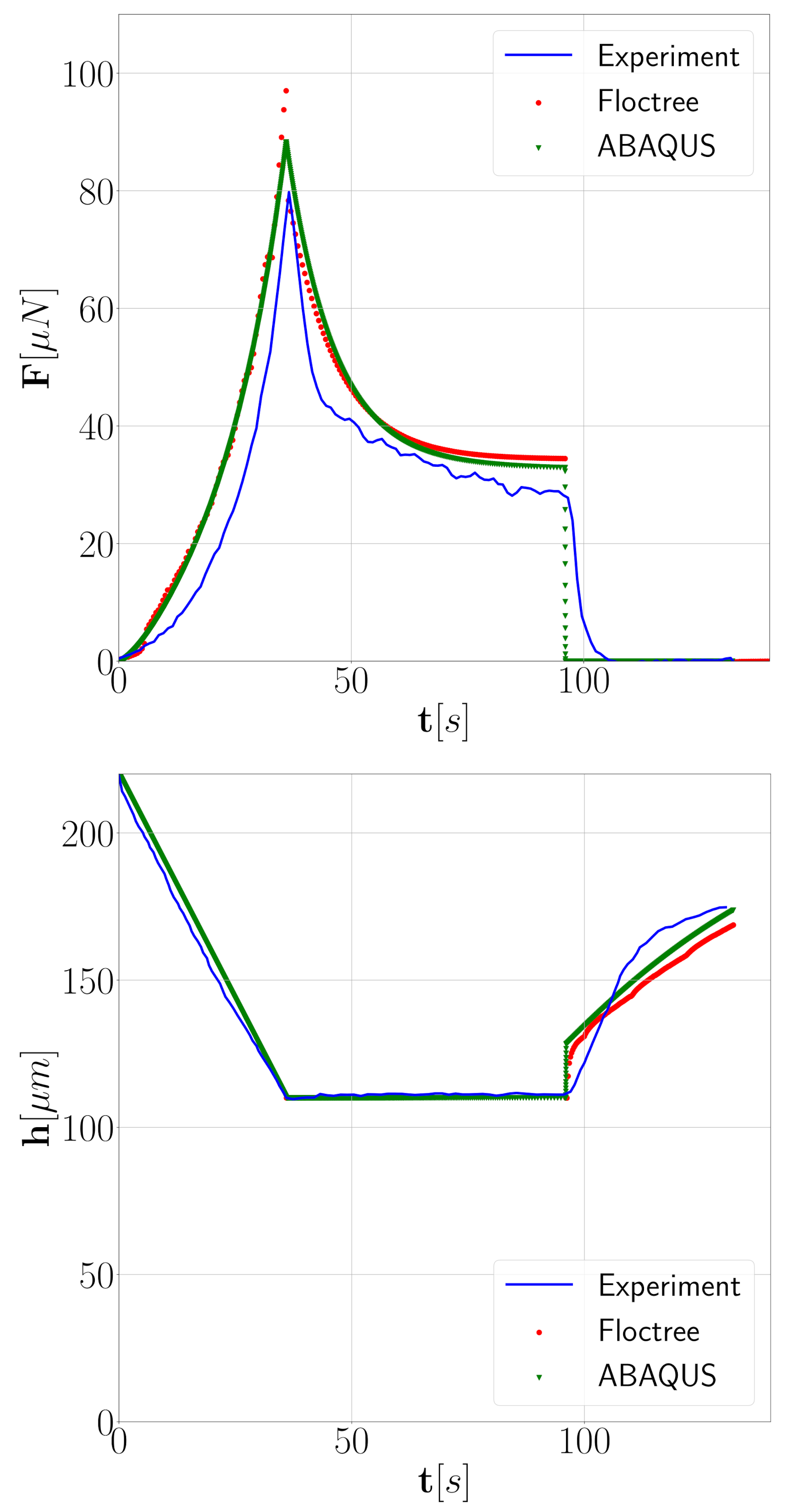
Figure 2 demonstrates the computed reaction force and the spheroid height for the case of instantaneous release and compares them with the physical experiment. To make the comparison between the solid and fluid viscoelastic models fair, we set the release phase duration in the ABAQUS simulation to be equal to the time step ($0.5$ s) for the fluid model.

We observe that the force and height graphs of both models are quite close. The instantaneous release of the plates results in the sharp increase of the spheroid height followed by a slower (than physically observed) gradual height increase in the remaining time. In contrast to the physical measurements, the simulated reaction force for both models vanishes instantaneously at $t=96$ since the upper and lower plates disappear according to the first scenario.

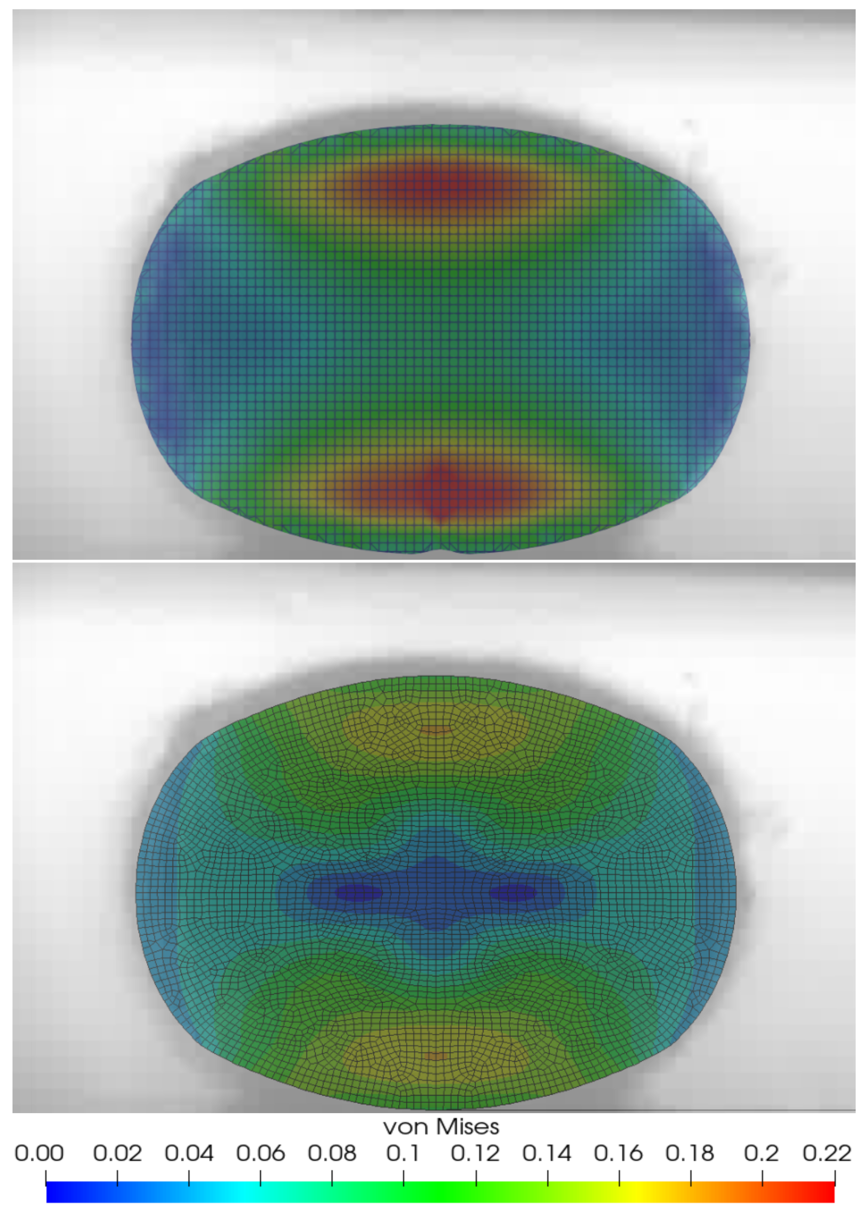
Despite the similarity of the reaction force and spheroid height graphs for both viscoelastic models, the distributions of the accumulated elastic energy differ. In Figure 3 we present the distributions of the elastic energy in terms of von Mises deviatoric stress $q=\sqrt{\frac{3}{2}(\mathrm{dev}\left[\overline{\mathit{\sigma }}\right]:\mathrm{dev}\left[\overline{\mathit{\sigma }}\right])}$ at the final time of the experiment $t=132$. Although the experimentally observed shape of the spheroid (shown in the background) matches the shapes computed by both models, the computed distribution of the elastic energy differ in the center of the spheroid.

The second scenario of our computational experiment addresses the physical experiment at the third phase when the upper plate is released slowly. The accurate solution of the solid–solid contact problem in the ABAQUS software allows us to simulate this scenario. In Figure 4, we compare the reaction force and the spheroid height graphs obtained by the viscoelastic solid model within both scenarios (instantaneous release and slow release) and the experimentally measured values. Under the slow release scenario, the computed reaction force matches the experimental one, whereas the computed spheroid height matches the measured one until $t\approx 105$ (see also the animated comparison of the results in the Supplementary Video S1).

The simulation of the slow release scenario based on the viscoelastic fluid model does not match the experiment. The main reason for the mismatch in the release phase is the inaccurate boundary condition at the contact surface. A more appropriate boundary condition is under development.

3.3. Discussion

We note that, although the viscoelastic solid model describes reasonably the multicellular spheroid compression, it can not be applied to the simulation of the MCSs fusion process manifesting extracellular matrix remodelling. Besides, experiments with the dissection of multicellular spheroids by a nanosecond laser scalpel suggest involvement of the surface tension phenomena. According to the recent study [44], simple models of the coalescence of highly viscous liquid drops with surface tension are not capable of correct description of the spheroids fusion process. The remedy may be provided by the direct simulation of the viscoelastic fluid with a free surface. The present study is devoted to the validation of such a model by the MCS compression experiment. Application of the presented viscoelastic fluid model to the MCSs fusion is a subject for the future research.

References

- Darling, E.M.; Topel, M.; Zauscher, S.; Vail, T.P.; Guilak, F. Viscoelastic properties of human mesenchymally-derived stem cells and primary osteoblasts, chondrocytes, and adipocytes. J. Biomech. 2008, 41, 454–464. [Google Scholar] [CrossRef] [Green Version]
- Lekka, M.; Pogoda, K.; Gostek, J.; Klymenko, O.; Prauzner-Bechcicki, S.; Wiltowska-Zuber, J.; Jaczewska, J.; Lekki, J.; Stachura, Z. Cancer cell recognition–mechanical phenotype. Micron 2012, 43, 1259–1266. [Google Scholar] [CrossRef]
- Efremov, Y.M.; Okajima, T.; Raman, A. Measuring viscoelasticity of soft biological samples using atomic force microscopy. Soft Matter 2020, 16, 64–81. [Google Scholar] [CrossRef]
- Hoffman, B.D.; Crocker, J.C. Cell mechanics: Dissecting the physical responses of cells to force. Annu. Rev. Biomed. Eng. 2009, 11, 259–288. [Google Scholar] [CrossRef]
- Verdier, C. Rheological properties of living materials. From cells to tissues. J. Theor. Med. 2003, 5, 67–91. [Google Scholar] [CrossRef]
- Gonzalez-Rodriguez, D.; Guevorkian, K.; Douezan, S.; Brochard-Wyart, F. Soft matter models of developing tissues and tumors. Science 2012, 338, 910–917. [Google Scholar] [CrossRef] [PubMed]
- Efremov, Y.M.; Zurina, I.M.; Presniakova, V.S.; Kosheleva, N.V.; Butnaru, D.V.; Svistunov, A.A.; Rochev, Y.A.; Timashev, P.S. Mechanical properties of cell sheets and spheroids: The link between single cells and complex tissues. Biophys. Rev. 2021, 13, 541–561. [Google Scholar] [CrossRef]
- Shafiee, A.; Norotte, C.; Ghadiri, E. Cellular bioink surface tension: A tunable biophysical parameter for faster maturation of bioprinted tissue. Bioprinting 2017, 8, 13–21. [Google Scholar] [CrossRef]
- Foty, R.A.; Forgacs, G.; Pfleger, C.M.; Steinberg, M.S. Liquid properties of embryonic tissues: Measurement of interfacial tensions. Phys. Rev. Lett. 1994, 72, 2298. [Google Scholar] [CrossRef] [PubMed]
- Chiara Giverso, C.; Di Stefano, S.; Preziosi, L. A three dimensional model of multicellular aggregate compression. Soft Matter 2019, 15, 10005–10019. [Google Scholar] [CrossRef]
- Preziosi, L.; Ambrosi, D.; Verdier, C. An elasto-visco-plastic model of cell aggregates. J. Theor. Biol. 2010, 262, 35–47. [Google Scholar] [CrossRef] [Green Version]
- Systèmes, D. ABAQUS Theory Guide. Version 6.14. 2014. Available online: http://130.149.89.49:2080/v6.14 (accessed on 29 July 2021).
- Bonito, A.; Picasso, M.; Laso, M. Numerical simulation of 3D viscoelastic flows with free surfaces. J. Comput. Phys. 2006, 215, 691–716. [Google Scholar] [CrossRef]
- Tomé, M.; Mangiavacchi, N.; Cuminato, J.; Castelo, A.; McKee, S. A finite difference technique for simulating unsteady viscoelastic free surface flows. J. Non-Newton. Fluid Mech. 2002, 106, 61–106. [Google Scholar] [CrossRef]
- Mompean, G.; Deville, M. Unsteady finite volume simulation of Oldroyd-B fluid through a three-dimensional planar contraction. J. Non-Newton. Fluid Mech. 1997, 72, 253–279. [Google Scholar] [CrossRef]
- Owens, R.G.; Phillips, T.N. Computational Rheology; World Scientific: Singapore, 2002. [Google Scholar]
- Oldroyd, J.G. On the formulation of rheological equations of state. Proc. R. Soc. Lond. Ser. A Math. Phys. Sci. 1950, 200, 523–541. [Google Scholar]
- Giesekus, H. A simple constitutive equation for polymer fluids based on the concept of deformation-dependent tensorial mobility. J. Non-Newton. Fluid Mech. 1982, 11, 69–109. [Google Scholar] [CrossRef]
- Thien, N.P.; Tanner, R.I. A new constitutive equation derived from network theory. J. Non-Newton. Fluid Mech. 1977, 2, 353–365. [Google Scholar] [CrossRef]
- Papanastasiou, A.; Scriven, L.; Macosko, C. An integral constitutive equation for mixed flows: Viscoelastic characterization. J. Rheol. 1983, 27, 387–410. [Google Scholar] [CrossRef]
- Luo, X.L.; Mitsoulis, E. An efficient algorithm for strain history tracking in finite element computations of non-Newtonian fluids with integral constitutive equations. Int. J. Numer. Methods Fluids 1990, 11, 1015–1031. [Google Scholar] [CrossRef]
- Alves, M.A.; Oliveira, P.J.; Pinho, F.T. Benchmark solutions for the flow of Oldroyd-B and PTT fluids in planar contractions. J. Non-Newton. Fluid Mech. 2003, 110, 45–75. [Google Scholar] [CrossRef]
- Alves, M.; Pinho, F.; Oliveira, P. The flow of viscoelastic fluids past a cylinder: Finite-volume high-resolution methods. J. Non-Newton. Fluid Mech. 2001, 97, 207–232. [Google Scholar] [CrossRef]
- Pan, T.W.; Hao, J.; Glowinski, R. On the simulation of a time-dependent cavity flow of an Oldroyd-B fluid. Int. J. Numer. Methods Fluids 2009, 60, 791–808. [Google Scholar] [CrossRef]
- Claus, S.; Phillips, T.N. Viscoelastic flow around a confined cylinder using spectral/hp element methods. J. Non-Newton. Fluid Mech. 2013, 200, 131–146. [Google Scholar] [CrossRef]
- Fang, J.; Owens, R.G.; Tacher, L.; Parriaux, A. A numerical study of the SPH method for simulating transient viscoelastic free surface flows. J. Non-Newton. Fluid Mech. 2006, 139, 68–84. [Google Scholar] [CrossRef] [Green Version]
- Rafiee, A.; Manzari, M.; Hosseini, M. An incompressible SPH method for simulation of unsteady viscoelastic free-surface flows. Int. J. Non-Linear Mech. 2007, 42, 1210–1223. [Google Scholar] [CrossRef]
- Xu, X.; Ouyang, J.; Jiang, T.; Li, Q. Numerical simulation of 3D-unsteady viscoelastic free surface flows by improved smoothed particle hydrodynamics method. J. Non-Newton. Fluid Mech. 2012, 177, 109–120. [Google Scholar] [CrossRef]
- Figueiredo, R.; Oishi, C.; Cuminato, J.; Alves, M. Three-dimensional transient complex free surface flows: Numerical simulation of XPP fluid. J. Non-Newton. Fluid Mech. 2013, 195, 88–98. [Google Scholar] [CrossRef]
- Viezel, C.; Tomé, M.; Pinho, F.; McKee, S. An Oldroyd-B solver for vanishingly small values of the viscosity ratio: Application to unsteady free surface flows. J. Non-Newton. Fluid Mech. 2020, 285, 104338. [Google Scholar] [CrossRef]
- Malaspinas, O.; Fiétier, N.; Deville, M. Lattice Boltzmann method for the simulation of viscoelastic fluid flows. J. Non-Newton. Fluid Mech. 2010, 165, 1637–1653. [Google Scholar] [CrossRef] [Green Version]
- Hirt, C.W.; Nichols, B.D. Volume of fluid (VOF) method for the dynamics of free boundaries. J. Comput. Phys. 1981, 39, 201–225. [Google Scholar] [CrossRef]
- Harlow, F.H.; Welch, J.E. Numerical calculation of time-dependent viscous incompressible flow of fluid with free surface. Phys. Fluids 1965, 8, 2182–2189. [Google Scholar] [CrossRef]
- Osher, S.; Fedkiw, R. Level Set Methods and Dynamic Implicit Surfaces; Springer Science & Business Media: Berlin/Heidelberg, Germany, 2006; Volume 153. [Google Scholar]
- Nikitin, K.; Vassilevski, Y.; Yanbarisov, R. An implicit scheme for simulation of free surface non-Newtonian fluid flows on dynamically adapted grids. Russ. J. Numer. Anal. Math. Model. 2021, 36, 165–176. [Google Scholar] [CrossRef]
- Lim, C.; Zhou, E.; Quek, S. Mechanical models for living cells—A review. J. Biomech. 2006, 39, 195–216. [Google Scholar] [CrossRef] [PubMed]
- Oh, M.J.; Kuhr, F.; Byfield, F.; Levitan, I. Micropipette aspiration of substrate-attached cells to estimate cell stiffness. J. Vis. Exp. JoVE 2012, 67, 3886. [Google Scholar] [CrossRef] [Green Version]
- Miller, K. Method of testing very soft biological tissues in compression. J. Biomech. 2005, 38, 153–158. [Google Scholar] [CrossRef] [PubMed]
- Martins, P.; Natal Jorge, R.; Ferreira, A. A comparative study of several material models for prediction of hyperelastic properties: Application to silicone-rubber and soft tissues. Strain 2006, 42, 135–147. [Google Scholar] [CrossRef]
- Kubo, R. Large elastic deformation of rubber. J. Phys. Soc. Jpn. 1948, 3, 312–317. [Google Scholar] [CrossRef]
- Rivlin, R. Large elastic deformations of isotropic materials. I. Fundamental concepts. Philos. Trans. R. Soc. Lond. Ser. A Math. Phys. Sci. 1948, 240, 459–490. [Google Scholar]
- Borzenok, S.; Saburina, I.; Repin, V.; Kosheleva, N.; Gorkun, A.; Komakh, Y.; Zheltonozhko, A. Methodological and technological problems of artificial cornea engineering based on 3D cellular cultivation. Oftal’mokhirurgiya 2012, 4, 12. [Google Scholar]
- Kosheleva, N.; Zurina, I.; Saburina, I.; Gorkun, A.; Kolokoltsova, T.; Borzenok, S.; Repin, V. The impact of fetal bovine serum on formation of spheroids from eye stromal limbal cells. Patogenez 2015, 13, 4. [Google Scholar]
- Kosheleva, N.V.; Efremov, Y.M.; Shavkuta, B.S.; Zurina, I.M.; Zhang, D.; Zhang, Y.; Minaev, N.V.; Gorkun, A.A.; Wei, S.; Shpichka, A.A.; et al. Cell spheroid fusion: Beyond liquid drops model. Sci. Rep. 2020, 10, 12614. [Google Scholar] [CrossRef] [PubMed]
- Repin, V.; Saburina, I.; Kosheleva, N.; Gorkun, A.; Zurina, I.; Kubatiev, A. 3D-technology of the formation and maintenance of single dormant microspheres from 2000 human somatic cells and their reactivation in vitro. Bull. Exp. Biol. Med. 2014, 158, 137–144. [Google Scholar] [CrossRef] [PubMed]
- Forgacs, G.; Foty, R.A.; Shafrir, Y.; Steinberg, M.S. Viscoelastic properties of living embryonic tissues: A quantitative study. Biophys. J. 1998, 74, 2227–2234. [Google Scholar] [CrossRef] [Green Version]
- Brodland, G.W.; Yang, J.; Sweny, J. Cellular interfacial and surface tensions determined from aggregate compression tests using a finite element model. HFSP J. 2009, 3, 273–281. [Google Scholar] [CrossRef] [Green Version]
- Omelyanenko, N.P.; Karalkin, P.A.; Bulanova, E.A.; Koudan, E.V.; Parfenov, V.A.; Rodionov, S.A.; Knyazeva, A.D.; Kasyanov, V.A.; Babichenko, I.I.; Chkadua, T.Z.; et al. Extracellular matrix determines biomechanical properties of chondrospheres during their maturation in vitro. Cartilage 2020, 11, 521–531. [Google Scholar] [CrossRef] [PubMed]
Figure 1.
Spheroid compression test.
Figure 2.
The reaction force acting on the upper plate (top) and the spheroid height (bottom) in the case of instantaneous release of the plates.
Figure 3.
Experimental spheroid shape at (background), viscoelastic fluid (top) and viscoelastic solid (bottom) elastic energy distribution in terms of von Mises deviatoric stress.
Figure 4.
The reaction force acting on the upper plate (top) and the spheroid height (bottom). Two scenarios of the release phase and experimental measurements.
Publisher’s Note: MDPI stays neutral with regard to jurisdictional claims in published maps and institutional affiliations. |
© 2021 by the authors. Licensee MDPI, Basel, Switzerland. This article is an open access article distributed under the terms and conditions of the Creative Commons Attribution (CC BY) license (https://creativecommons.org/licenses/by/4.0/).
Share and Cite
MDPI and ACS Style
Yanbarisov, R.; Efremov, Y.; Kosheleva, N.; Timashev, P.; Vassilevski, Y. Numerical Modelling of Multicellular Spheroid Compression: Viscoelastic Fluid vs. Viscoelastic Solid. Mathematics 2021, 9, 2333. https://doi.org/10.3390/math9182333
AMA Style
Yanbarisov R, Efremov Y, Kosheleva N, Timashev P, Vassilevski Y. Numerical Modelling of Multicellular Spheroid Compression: Viscoelastic Fluid vs. Viscoelastic Solid. Mathematics. 2021; 9(18):2333. https://doi.org/10.3390/math9182333
Chicago/Turabian StyleYanbarisov, Ruslan, Yuri Efremov, Nastasia Kosheleva, Peter Timashev, and Yuri Vassilevski. 2021. "Numerical Modelling of Multicellular Spheroid Compression: Viscoelastic Fluid vs. Viscoelastic Solid" Mathematics 9, no. 18: 2333. https://doi.org/10.3390/math9182333
Note that from the first issue of 2016, this journal uses article numbers instead of page numbers. See further details here.