
An Auditory Saliency Pooling-Based LSTM Model for Speech Intelligibility Classification


1
Department of Signal Theory and Communications, Universidad Carlos III de Madrid, Avda. de la Universidad, 30, Leganés, 28911 Madrid, Spain
2
Speech Technology Group, E.T.S.I. Telecomunicación, Universidad Politécnica de Madrid, Avda. de la Complutense, 30, 28040 Madrid, Spain
*
Author to whom correspondence should be addressed.
Symmetry 2021, 13(9), 1728; https://doi.org/10.3390/sym13091728
Submission received: 7 August 2021
/
Revised: 12 September 2021
/
Accepted: 16 September 2021
/
Published: 18 September 2021
(This article belongs to the Section Computer)
Abstract
:Speech intelligibility is a crucial element in oral communication that can be influenced by multiple elements, such as noise, channel characteristics, or speech disorders. In this paper, we address the task of speech intelligibility classification (SIC) in this last circumstance. Taking our previous works, a SIC system based on an attentional long short-term memory (LSTM) network, as a starting point, we deal with the problem of the inadequate learning of the attention weights due to training data scarcity. For overcoming this issue, the main contribution of this paper is a novel type of weighted pooling (WP) mechanism, called saliency pooling where the WP weights are not automatically learned during the training process of the network, but are obtained from an external source of information, the Kalinli’s auditory saliency model. In this way, it is intended to take advantage of the apparent symmetry between the human auditory attention mechanism and the attentional models integrated into deep learning networks. The developed systems are assessed on the UA-speech dataset that comprises speech uttered by subjects with several dysarthria levels. Results show that all the systems with saliency pooling significantly outperform a reference support vector machine (SVM)-based system and LSTM-based systems with mean pooling and attention pooling, suggesting that Kalinli’s saliency can be successfully incorporated into the LSTM architecture as an external cue for the estimation of the speech intelligibility level.
1. Introduction
Speech intelligibility refers to the comprehensibility of speech and its deterioration can drastically hinder the communication process between speaker and listener. The speech intelligibility level (SIL) may deteriorate due to a variety of reasons, such as the presence of environmental noise, channel distortions, or physiological impairments in the human speech production system caused by certain sicknesses or other causes that produce the so-called disordered or pathological speech.
This work focuses on the task of speech intelligibility classification (SIC) for dysarthric speech that is a particular case of pathological voice. The term dysarthria refers to a speech disorder caused by the impaired movement of the speech muscles [1], and is characterized by vocal harshness, nasality, deficient articulation, unclear coarticulations between phonemes, excessive phoneme duration, and disturbances in the intensity, pitch, and elocution speed [2,3]. It is a typical symptom and consequence of several degenerative illnesses, such as amyotrophic lateral sclerosis, Huntington’s Disease, or Parkinson’s Disease.
The assessment of the SIL has multiple practical applications, such as the monitoring of patients following logopedic or other medical therapies, and the aid to diagnosis and the tracking of the progression of several illnesses, such as the aforementioned Parkinson’s Disease or the Alzheimer Disease.
The most commonly used method for judging the SIL is based on subjective tests where specialists listen to several words uttered by the patient and annotate the percentage of words correctly understood, obtaining the so-called intelligibility score. However, this is a time-consuming task and is hampered by the hearing skills and subjective criterion of the clinicians [4]. For these reasons, in recent years, the automatization of this task has attracted the attention of numerous researchers with the aim of obtaining a less variable and reproducible measure for the speech intelligibility.
Many of the SIC systems proposed in the literature are based on classical machine learning algorithms, such as, for example, linear discriminant analysis [3,5,6], support vector machines (SVM) [7,8,9], or random forests [10], that use, as input, different types of hand-crafted features, such as the average of the mel frequency cepstrum coefficients (MFCC) [8,11], the average of the mel-frequency delta-energy coefficients [12], the intensity and frequency of the maximum values of the modulation spectrum [5], the quotient between low and high modulation energies [3,6], the average energy of the modulation spectrogram [8] or features derived from the output of an automatic speech recognizer [9,13].
More recently, deep learning (DL) methods have been proposed for SIC as they have been proven to be very effective in several audio and speech-related tasks, such as acoustic event detection [14], automatic speech recognition [15], speech emotion recognition [16,17,18], cognitive load classification from speech [19,20], or deception detection from speech [21]. Recent studies propose the use of dense networks fed by features derived from the decomposition of log-mel spectrograms in temporal and frequency basis vectors [22], the use of convolutional neural networks and different spectro-temporal representations as input [23], or long short-term memory (LSTM) networks with MFCC as feature vectors [24] for multilevel or binary speech intelligibility classification.
LSTMs can be integrated with weighted pooling (WP) mechanisms with the aim of obtaining a compact representation of the whole utterance, that is fed to the classifier itself. Attention pooling [16,25,26] is a recently proposed WP scheme that, incorporated into the conventional LSTM, is able to perform a better modeling of the input sequences by learning the relevance scores (weights) of the temporal frames, and by modulating the contribution of each temporal frame to the final output as a function of its score.
Our previous works on SIC, where we addressed the problem of estimating the speech intelligibility level of a dysarthric patient, can be placed in this latter approach. In [8], we proposed a SIC system based on per-frame log-mel spectrograms and attention LSTM networks that significantly outperformed a SVM-based system with hand-crafted features. Furthermore, in [11] we showed that this architecture is also suitable for the modeling of per-frame modulation spectrograms [27] and that the combination of log-mel and modulation spectrograms into an attentional LSTM framework outperforms the corresponding individual systems.
The main weakness of our previous research is that the lack of training data (typical in this kind of medical applications) prevents the use of complex attention models as it is not feasible to properly train them. For this reason, we were restricted to using simpler models, and were unable to exploit all the possibilities of this technique. For overcoming this issue, in this paper, we study the alternative of using external sources of information to establish the weights of the WP stage of the LSTM-based system instead of learning them during the network training. In particular, we propose to compute these weights from the so-called saliency that is produced by an external auditory saliency model. This approach is called saliency pooling. In [19], we presented preliminary experiments on cognitive load estimation from speech using a system based on a similar strategy. Here, we deepen into this approach and we apply it to the task of SIC, what, to the best of our knowledge, has not been studied before.
From a more general psychological perspective, saliency and attention are related concepts. Attention refers to a cognitive function that prioritizes particular stimuli over others [28], allowing persons to choose the most important events in their surroundings in order to concentrate their cognitive and sensory capabilities on them. It is clear that there is a conceptual symmetry between the human attention mechanism and the aforementioned attention models that are integrated into DL-based systems [26]. When attention is modulated by bottom-up, sensory-driven factors, it is denoted as saliency. Particularizing to the case of audition, the auditory saliency mechanism is able to detect the sounds that constitute conspicuous or salient events of a complex acoustic scene, by focusing on acoustic cues, such as intensity or timbre [29].
In recent years, several models of auditory saliency have been proposed [30,31,32,33,34]. Among them, in this work, we have considered the auditory saliency model developed by Kalinli et al. [35,36,37] as it is inspired on the central auditory system and has been successfully tested for prominent syllable detection in speech. As demonstrated in [38], listeners can perceive a phoneme or syllable to be more salient than the others due to several circumstances, such as the stress, intensity, or coarticulation between adjacent phonemes. As aforementioned, speech intelligibility can be reflected in some way in these phenomena [2,3], so our hypothesis is that Kalinli’s model can help to detect the salient parts of speech that are more relevant to the determination of the comprehensibility level of an utterance, and, therefore, it is feasible to use it as a kind of weighted pooling model inside our LSTM-based SIC system.
This research aims to improve our previously developed attention LSTM-based SIC system by addressing the problem of the inadequate learning of the attention weights due to training data scarcity. This work is supported by the hypothesis that, in these situations, it is more effective to introduce external cues to the LSTM architecture in order to obtain these weights. In this sense, the main contribution of this paper is the so-called saliency pooling where the WP weights are derived from the saliency values produced by an external auditory saliency model, in particular, the Kalinli’s model. This approach can be seen as a method for emphasizing the more relevant frames of the input features (in this case, log-mel spectrograms) that can be easily integrated into the LSTM framework.
The remainder of the document is structured as follows: Section 2 describes the dataset utilized in the experiments, the auditory saliency model and the proposed LSTM-based systems for speech intelligibility classification. In addition, it contains the experimental protocol and the evaluation measures used for the assessment of the different systems. Section 3 and Section 4 include, respectively, the main results and the corresponding discussion and future work. Section 5 closes the document with some conclusions.
2. Materials and Methods
2.1. Database
In this work, we have utilized the UA-speech database [39] that contains speech uttered by 11 male and 4 female patients with different levels of dysarthria. Each participant pronounced 765 isolated words of several complexities (digits, radio alphabet letters, commands, common short words, and uncommon long words). The audio files were collected with an array of 7 microphones and a sampling frequency of 16 KHz. Only signals acquired with the 6th microphone have been used in the experiments. As several files were discarded due to errors in the recording process, the total number of available exemplars is 11,435.
The dataset was manually labeled in terms of the intelligibility score by medical staff who performed several listening tests and annotated the percentage of understood words for each participant. As the values of these original scores were in the range from 0 to 100, they were transformed to the three intelligibility levels considered in this study: low (scores from 0 to 33), medium (from 34 to 66), and high (from 67 to 100).
2.2. Auditory Saliency Model
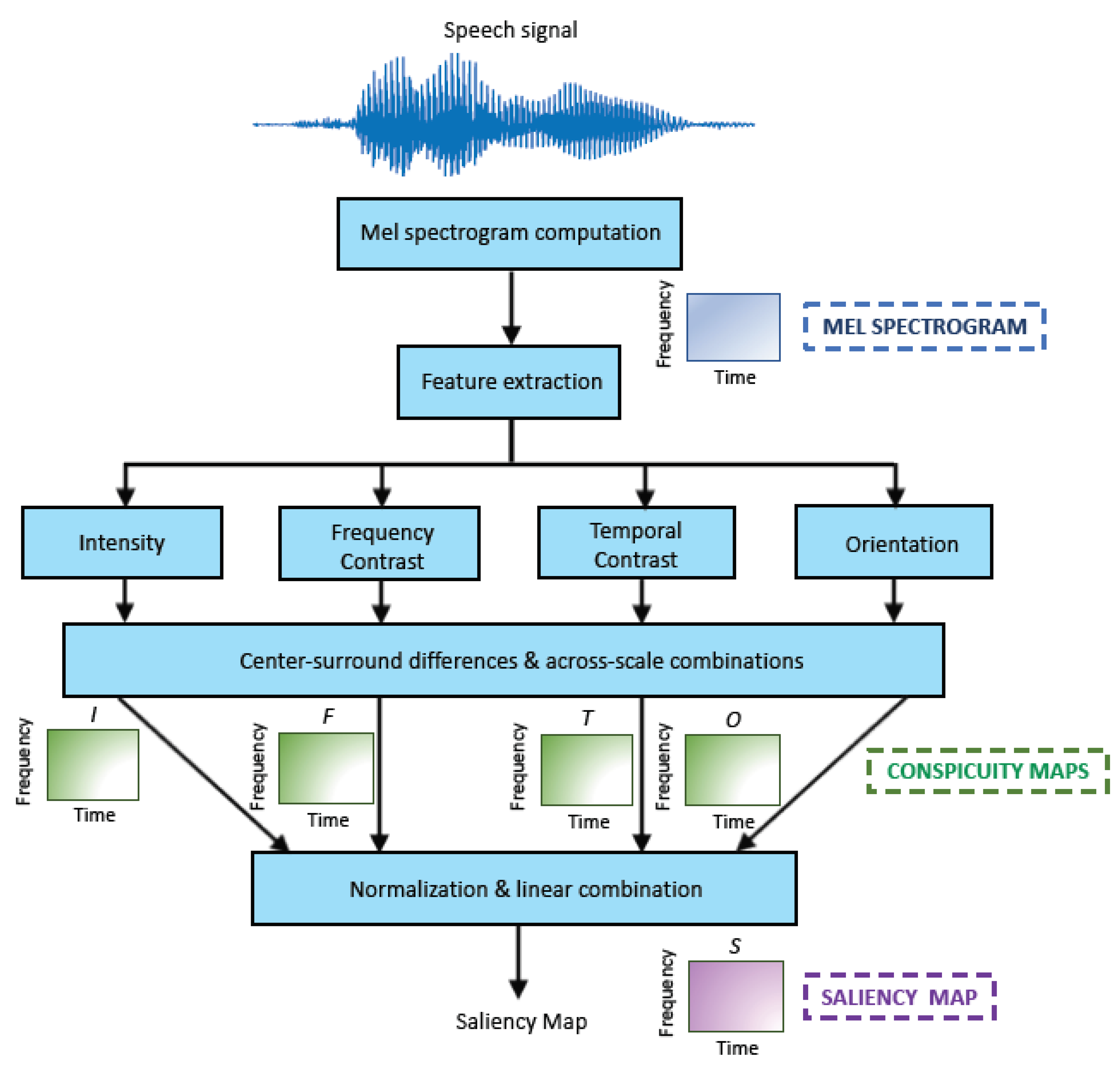
In order to compute the saliency values of the speech signals, in this work we have used the Kalinli’s model [35,36,37], as implemented in [40]. Its simplified block diagram is represented in Figure 1.
The process is as follows. First, a two-dimensional (2D) spectro-temporal representation of the speech signal, called mel spectrogram, is computed using an analysis Hamming window of 32 ms length with an overlap between adjacent windows of (i.e., the frame period is ms) and an auditory filterbank composed of 256 triangular mel-scaled filters. The mel scale is a frequency transformation that mimics the sensitivity of the human auditory system at different frequencies. The dimension of the resulting mel spectrogram is , where is the number of mel filters (256 in this case) and is the number of acoustic frames, being each of them equivalent to ms.
This mel spectrogram is further processed by extracting four features (intensity, frequency, and temporal contrast and orientation). For doing that, a set of receptive filters that simulates the analysis carried out in the primary auditory cortex [41] is utilized. These features are computed at multiple scales, each being a decimated version by a factor 2 of the previous one. Then, center-surround differences are computed and the different scales are combined resulting in a set of conspicuity maps , where , , , denote, respectively, the intensity, frequency contrast, temporal contrast, and orientation conspicuity maps. As the number of scales is four, the final dimension of these maps is 1:8 of the original size of the input mel spectrogram. Therefore, the dimension of is , where and , i.e., the frame period is now ms × ms.
These maps are normalized by using an iterative and non-linear algorithm [35,36,37] that emphasizes their most prominent areas, and summed up, as follows,
yielding the final 2D auditory saliency map with size .
The weights that are incorporated as an external source of information into the WP stage of the LSTM-based SIC system are derived from both, the conspicuity and saliency maps, as described in Section 2.3.2.
2.3. Many-to-One LSTM Networks
Following our previous works on speech intelligibility classification [8,11], the SIC system is based on long short-term memory networks [42,43].
In this case, LSTM works in a many-to-one mode because in the SIC task a single output (intelligibility level) must be assigned to the whole input sequence. Specifically, in a first step, LSTM processes a T-long input sequence , transforming it into a T-long output sequence , and in a second step, Y is summarized in a single value Z by means of a certain weighted pooling (WP) mechanism [16,44]. Finally, Z is the input to the classifier itself.
The WP stage is implemented as the linear combination of the frames of the LSTM output sequence, according to the following expression,
where is the set of weights that determines the contribution of each LSTM frame to Z, and is computed following a certain criterion, that, at least in theory, should be related to the relevance of the frame to the classification task.
Two relevant methods of WP are mean pooling (MP), where the weights are the same for all frames and equal to [17], and attention pooling (AP) that is going to be described in next paragraphs together to our approach, denoted as saliency pooling (SP).
2.3.1. Attention Pooling
The rationale behind this strategy is that not all the LSTM frames convey the same useful information for the classification task in hand and, therefore, the more relevant ones should be emphasized by means of the assignment of weights with high values. In contrast, non-relevant frames should be diminished or even ignored, so the values of the corresponding weights should be small. This approach has been proposed with great success in other automatic learning problems that deal with temporal sequences [14,16,17,19,20,21,25,45], including our previous works on the estimation of the intelligibility level [8,11].
The availability of large amounts of training data makes feasible to utilize complex attention models, as those proposed in [16,44]. However, as in our case the training data are scarce, we have adopted the strategy proposed, among others, by [17]. This is a simple model, and for that, it is more appropriate for this kind of scenarios. This way, the attention weights are computed through the following Equation:
where stands for the transpose operation, and u is a learnable attention parameter that is computed during the training process of the system. Note that Equation (3) involves a softmax transformation, in such a way that the summation of the sequence weights is equal to one.
2.3.2. Saliency Pooling
Attention and saliency pooling share the same basic hypothesis about the uneven importance of each temporal frame. However, they differ in the way the weights are computed.
As aforementioned, the training data scarcity makes the use of sophisticated attention models inappropriate. Our assumption is that, in this situation, the attentional mechanism described in Section 2.3.1, even being simple, is not going to be properly learned during the training process and, as a consequence, it should be more adequate to obtain the weights from external sources of information.
As pointed out in Section 2.2, in the SP approach, the conspicuity and saliency maps produced by the Kalinli’s auditory saliency model are considered as external cues for finding out the relevance score for each temporal frame. Our hypothesis is that frames containing relevant information for the determination of the utterance intelligibility level can be identified with the help of this saliency analysis. This way, a frame with a large conspicuity or saliency value should also present a large weight into the WP scheme.
We have computed five different variants of saliency weights (note that throughout this paper, all the weights derived from the Kalinli’s auditory saliency model are referred to as saliency weights, regardless of whether they have been computed from conspicuity or saliency maps.). The first four ones are derived from the four conspicuity maps (, , , and ), and are referred to as Intensity, Frequency Contrast, Temporal Contrast, and Orientation weights, respectively. The last set is computed from the saliency map () and is denoted as Global Saliency weights.
The process for obtaining any of these sets of weights is as follows. Firstly, as conspicuity and saliency maps are 2D representations and the weights are unidimensional temporal signals, these maps are summed across frequency channels for each time instant [46]. Secondly, the resulting vectors are standardized at utterance-level to mean zero and standard deviation one, obtaining a saliency signal of length T, . Finally, the saliency weights are obtained by applying the softmax transformation on the saliency signal, using the following Equation:
Note that, as in the case of the attention weights described in Section 2.3.1, the saliency weights also add up to one.
2.4. Speech Intelligibility Classification System
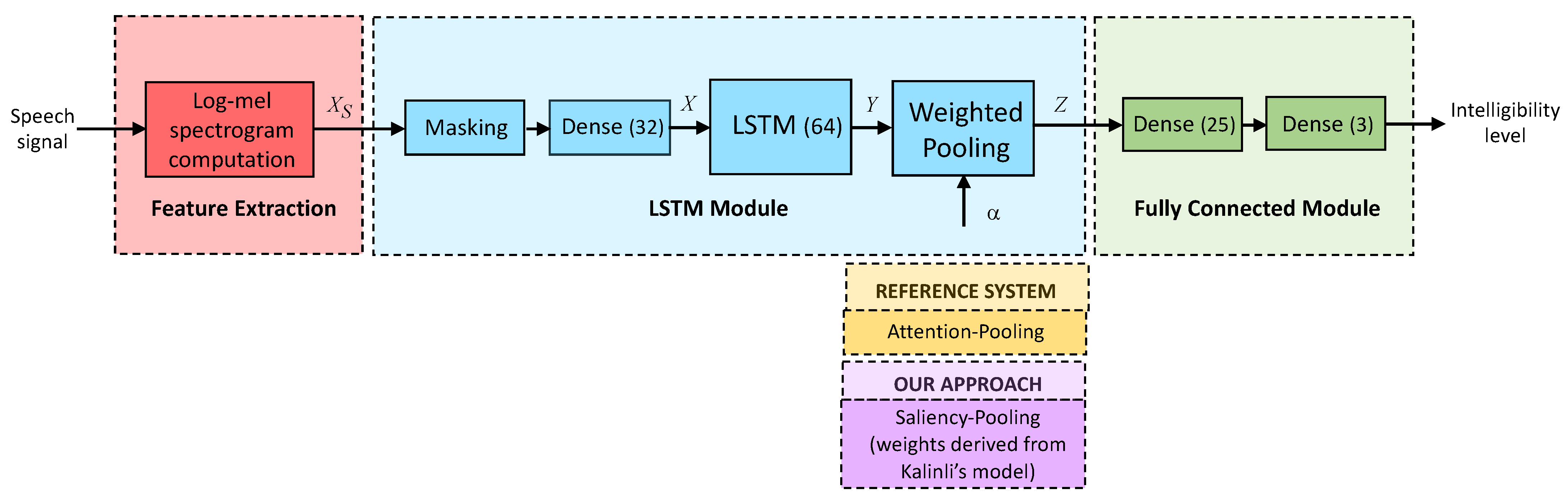
Figure 2 shows the block diagram of the SIC system developed in this work, whose main stages are described in next subsections.
2.4.1. Feature Extraction
The input to the SIC system consists of log-mel spectrograms, a kind of 2D speech representations that have been previously used for this task [8,11,21], and other applications related to speech and audio processing, such as depression detection [47], deception detection [21], or sound classification [48].
Log-mel spectrograms are computed in a similar way to the mel spectrograms described in Section 2.2, but in this case a 20 ms Hamming window with a 10 ms overlap is used. In addition, the outputs of the auditory filterbank are later converted to a logarithmic scale. The Python’s package LibROSA [49] is utilized for this purpose.
Then, for each utterance, these features are standardized to mean zero and variance one, yielding a normalized sequence whose dimension is , where and T are, respectively, the number of mel filters (32 in this case) and speech frames. These acoustic frames are extracted every 10 ms, matching the frame period of conspicuity and saliency maps, and saliency signals).
To optimize the computational resources required by LSTM networks, the input sequences must be of the same duration. For this reason, taking into account that more than of the speech signals are shorter than 7 s, a maximum length of frames was established (see [8] for details). Sequences longer than this quantity were cut, whereas shorter ones were completed with dummy values that are discarded in subsequent computations.
2.4.2. LSTM and Fully Connected Modules
The LSTM module is composed of a masking layer that guarantees that the masked values of the padded input sequences are not utilized in subsequent processes (see Section 2.4.1), a dense layer of 32 neurons and a LSTM layer with 64 hidden units connected to a weighted pooling step. As mentioned before, two different techniques for WP have been tested: attention pooling and our approach, saliency pooling.
The WP output goes into the fully connected module, that is composed of a dense layer of 25 neurons with a dropout of in order to avoid over-fitting during the network training, and a final dense layer with a sigmoid activation function. This last layer has 3 nodes as the number of possible intelligibility categories is also 3 (low, medium, and high).
2.5. Experimental Protocol and Assessment Measures
All the tested models were built with the Python’s packages Tensorflow [50] and Keras [51]. These systems were trained with the Adam optimizer and a categorical cross-entropy loss function with the following values of the learning rate, the batch size and the maximum number of epochs: , 32, and 50.
We used the same experimental protocol as in our previous work [11], consisting of a subject-independent 5-fold cross validation. Specifically, the database was split into five balanced groups. In each one of the five sub-experiments, three groups composed the training set, whereas the remainder two groups were used as, respectively, the validation and testing sets. These three sets were disjoint in the sense that a speaker was included in only one of them. This way, it was avoided that the systems learned the speaker’s identity instead of his or her comprehensibility degree. Results corresponds to the average of these five sub-experiments.
For the systems assessment, we adopted the accuracy or classification rate per speech file as evaluation metric. It is defined as the ratio between correctly classified audio recordings and the total amount of test files. As each experiment was repeated 20 times, results included in Section 3 correspond to the average and standard deviation of the classification rate across these 20 experiments.
3. Results
Table 1 contains the mean and standard deviation of the accuracies obtained with the LSTM-based systems with the two weighted pooling schemes studied in this work: attention pooling and the five variants of saliency pooling. For comparison purposes, the accuracy obtained by the LSTM-based system with mean pooling is also reported. Note that MP can be considered as a special case of WP where the weights of all temporal frames are equal, i.e., all the frames are assumed to be evenly relevant to the task. In addition, for completeness, the outcome achieved by a traditional machine learning algorithm (in particular, a SVM) that uses the average of the MFCC as input is also included. More details about the implementation of this last system can be consulted in our previous work [11]. Moreover, a set of preliminary experiments were performed where conspicuity/saliency maps were directly fed to the LSTM system instead of log-mel spectrograms. Results were worse than in the case of the baseline LSTM system with log-mels and AP and, for brevity reasons, they have not been included here. Any case, this outcome suggests that conspicuity/saliency maps do not carry out enough information for the SIC task by themselves, being more adequate the use of the SP approach proposed in this work, as shown in this Section.
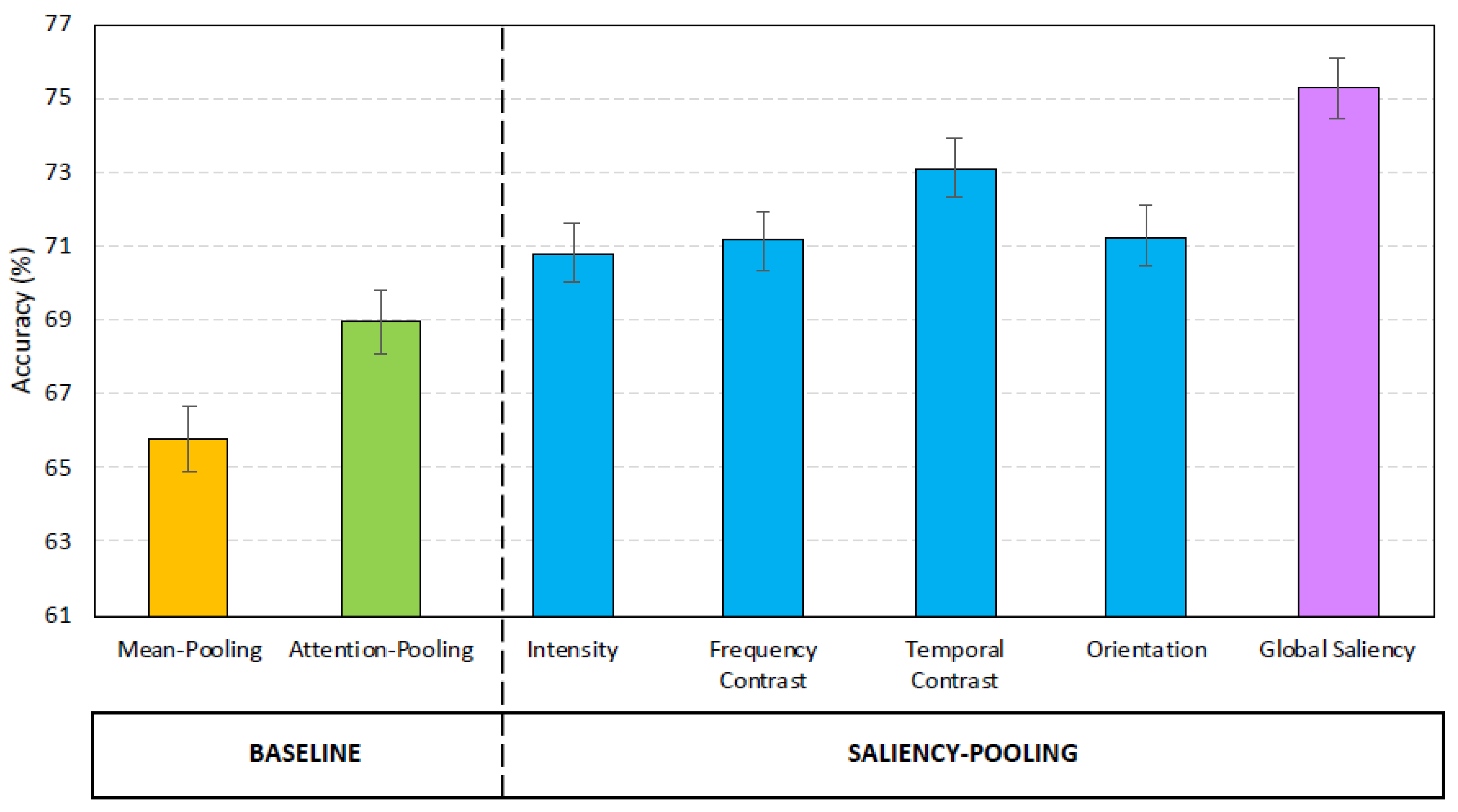
Figure 3 shows the mean accuracies achieved by the LSTM-based architectures assessed in this study, and the corresponding 95% confidence intervals. For a better visualization, the SVM-based system is not included in this graph.
Firstly, as expected, all LSTM-based systems achieve better classification rates than the SVM-based one. This result confirms our previous findings related the comparison between traditional machine learning and deep learning techniques [11] for the SIC task.
Secondly, focusing on the different WP schemes, mean pooling achieves the worst performance. Attention pooling produces better results than this basic approach, since it allows the system to automatically learn the speech frames that contribute the most to the determination of the intelligibility level of the utterance. Nevertheless, this strategy does not seem effective enough as it is outperformed by all the variants of saliency pooling, where the relevance score of each temporal frame is estimated from an external information source, that in this case is the Kalinli’s auditory saliency model. In addition, the differences in performance between attention pooling and saliency pooling are statistically significant.
Thirdly, as for the comparison between the different SP techniques, it can be observed that the classification rates achieved by Intensity, Frequency Contrast, and Orientation are very similar, whereas Temporal Contrast produces significantly better results than these three former variants.
Finally, the best system is Global Saliency, where the weights of the temporal frames are computed from the saliency map that is a linear combination of the four conspicuity maps. In particular, Global Saliency obtains a relative error reduction of with respect to Temporal Contrast, of with respect to attention pooling, of with respect to mean pooling, and of with respect to SVM.
4. Discussion
Results corroborate the main hypothesis of this paper that points out the feasibility of using an auditory saliency model, the Kalinli’s model, to determine the frames conveying the most relevant information about the intelligibility level of an utterance, in such a way that the saliency signal can be incorporated as an external cue into the weighted pooling stage of a LSTM-based system for the SIC task.
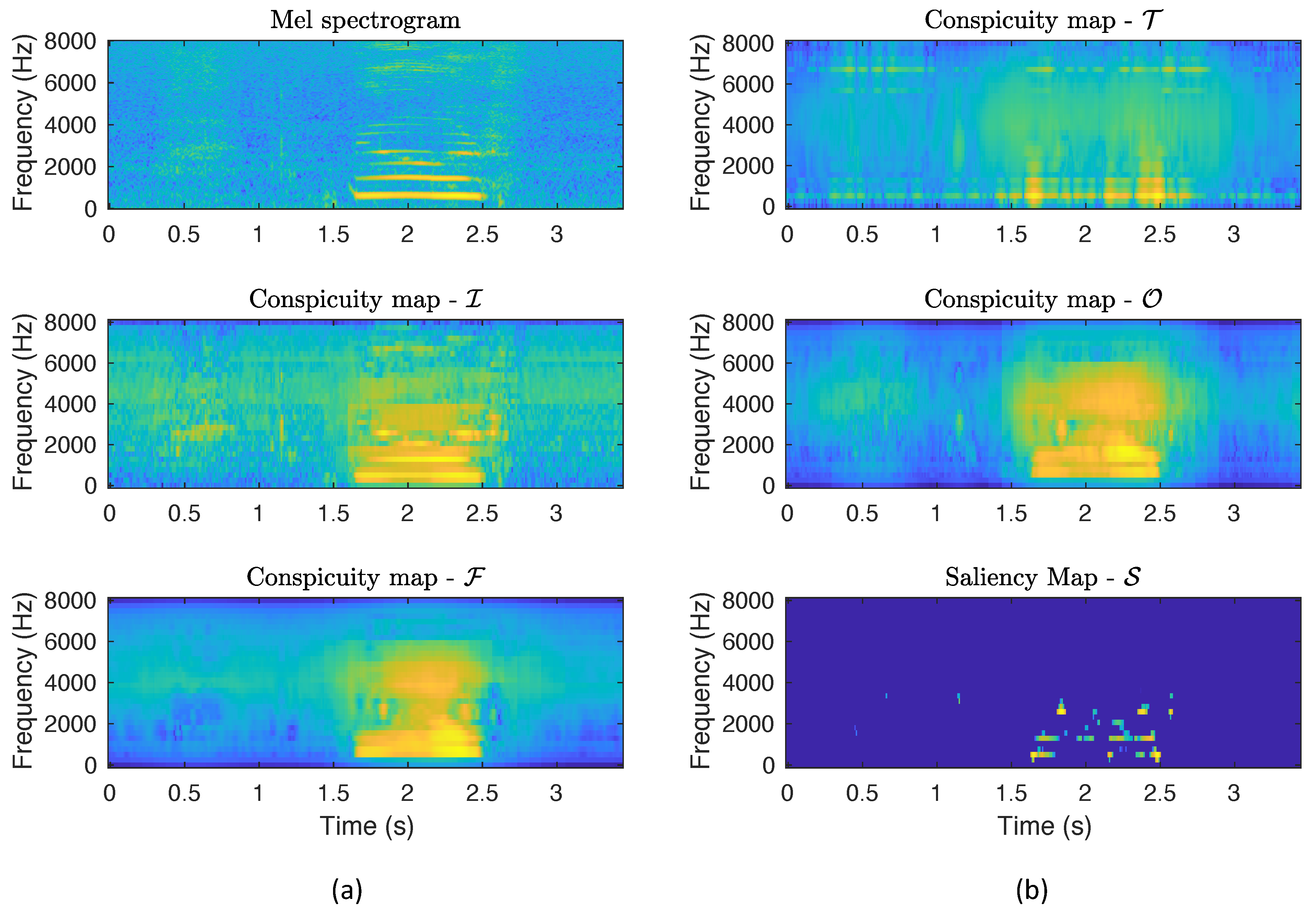
In order to gain more insight into the performance of the proposed LSTM-based systems, the behaviour of the auditory saliency model and the SP mechanism is illustrated in the next example.
Figure 4 shows the conspicuity and saliency maps produced by the Kalinli’s model over an utterance of low intelligibility belonging to the UA-SPEECH database. This speech signal consists of a hesitation between s and 1 s and the word “jowls” between s and s. In particular, Figure 4a represents from top to bottom, the mel spectrogram, the Intensity and the Frequency Contrast conspicuity maps, whereas Figure 4b depicts the Temporal Contrast and Orientation Conspicuity maps, and the saliency map. On the one hand, it can be observed that Intensity, Frequency Contrast, and Orientation maps are similar, whereas the Temporal Contrast one presents a different structure, being the more conspicuous regions of this map mainly located in the coarticulations (around s and s). In addition, the four conspicuity maps present a certain degree of relevant regions placed in the hesitation event, although it is not a proper speech sound. On the other hand, the saliency map is more abrupt, exhibiting a smaller number of salient regions, all of them belonging to the region where the word “jowls” is located. Note that, in the remaining parts of the utterance, including the hesitation event, there is no salient regions. This fact is due to the normalization algorithm applied on the individual conspicuity maps, prior to their combination to build the final saliency map, that completely removes areas with very low conspicuity values.
Figure 5a,b show the waveform, attention pooling, Intensity, Frequency Contrast, Temporal Contrast, Orientation, and Global Saliency weights corresponding to the same utterance as in Figure 4. Additionally, mean pooling weights are depicted for comparison purposes. As a general observation, it can be seen that the AP and SP weights vary significantly with time, whereas the MP ones are constant, suggesting that the information about the intelligibility level of an utterance is regionalized and as a consequence, it seems crucial to detect the relevant frames to the SIC task and emphasize their contribution.
As for the comparison between the AP and SP mechanisms, it can be observed that the former assigns large weights to the areas corresponding to the hesitation event and the noise situated at the end of the word, that are not proper speech sounds and, therefore, they should not be taken into account, whereas the SP weights are smaller or even zero in these regions. This observation might justifies the fact that the results obtained by AP are worse than those achieved by SP.
Regarding the different SP variants, SP weights exhibit the same trends as the corresponding conspicuity and salience maps represented in Figure 4. Again, Intensity, Frequency Contrast, and Orientation weights are similar and they mainly spread over the speech sound segment. However, Temporal Contrast weights are more peaky and focus mainly to temporal transitions, such as coarticulations, that are known to carry information about the utterance intelligibility level [2,3]. This fact explains the better performance of Temporal Contrast over Intensity, Frequency Contrast, and Orientation SP variants. Any case, all these methods assign small non-zero relevance scores to the hesitation and background noise events.
In contrast, Global Saliency weights combine the detection capabilities of Temporal Contrast SP with the ability of entirely discarding frames corresponding to non-speech sounds. It is very plausible that this is the reason why Global Saliency SP is the method that produces the best results.
Limitations and Future Research
The automatic classification of the speech intelligibility level is a challenging task, even for humans, for several reasons. Firstly, it depends on the phonetic characteristics of the utterances used for measuring the intelligibility level (short, long, highly confusable words, etc.). Secondly, in the case of subjective tests carried out by specialists, the intelligibility assessment is influenced by the degree of familiarity with disordered speech experimented by the listener and his or her hearing skills. Thirdly, the presence of background noise in the recordings can alter the perception of the speech, making even more difficult its comprehensibility. Fourthly, the limited amount of data in the available datasets and its scarce diversity with respect to the distribution of intelligibility scores, age and gender directly affects the quality of the machine learning-based systems developed for this task [8,9].
All these elements cause that the SIC systems performance is far from optimal, giving place to new opportunities of research in this field. Specifically, for further work, we plan to study the selection of the optimum set of words for automatic intelligibility measurement, taking as starting point both, the analysis of the classification errors and the taxonomy of the salient areas detected by the auditory saliency model. Furthermore, taking into account that collecting and annotating new recordings for this task is very tough, we will study the more appropriate data augmentation methods for alleviating the problem of data scarcity. In addition, we will explore the use of new speech representations, such as the deep features derived from the decomposition of log-mel spectrograms in temporal and frequency basis vectors proposed in [22], and their combination with the saliency pooling LSTM-based model.
5. Conclusions
In this study, we have expanded our previous works about speech intelligibility classification based on attention LSTM networks. Specifically, we have addressed the problem of the inadequate learning of the attention weights due to training data scarcity. In this sense, our main contribution is a novel type of weighted pooling mechanism, called saliency pooling that is inspired on the symmetry between the human auditory attention mechanism and the fundamentals of the attention models integrated into deep learning networks. In this novel approach, the WP weights are not automatically learned during the training process of the network, but are obtained from an external source of information, the Kalinli’s auditory saliency model. The proposed technique can be seen as a method for emphasizing the more important frames of the log-mel spectrograms regarding the SIC task, that can be successfully incorporated into the LSTM architecture.
We have proposed five different variants of saliency pooling, four of them derived from the four conspicuity maps produced by the Kalinli’s model and the fifth one computed from the global Kalinli’s saliency map. The different systems have been assessed on the UA-speech dataset that comprises speech uttered by subjects with several dysarthria levels. All the systems with SP significantly outperform a traditional machine learning method (in particular, a SVM), a LSTM-based system with mean pooling and a LSTM-based system with attention pooling. These results show that saliency can be successfully incorporated into the LSTM architecture as an external cue for the estimation of the speech intelligibility level. Moreover, the system that achieves the best results is that it uses the global saliency weights. In particular, this model obtains a relative error reduction of with respect to SVM, of with respect to mean pooling, and with respect to attention pooling.
Author Contributions
Conceptualization, A.G.-A. and J.M.M.; methodology, A.G.-A. and J.M.M.; software, A.G.-A.; formal analysis, A.G.-A. and J.M.M.; investigation, A.G.-A. and J.M.M.; data curation, A.G.-A.; writing—original draft preparation, A.G.-A.; writing—review and editing, A.G.-A. and J.M.M.; funding acquisition, A.G.-A. and J.M.M. Both authors have read and agreed to the published version of the manuscript.
Funding
The work leading to these results has been supported by the Spanish Ministry of Economy, Industry and Competitiveness through TEC2017-84395-P (MINECO) and TEC2017-84593-C2-1-R (MINECO) projects (AEI/FEDER, UE), and the Universidad Carlos III de Madrid under Strategic Action 2018/00071/001.
Institutional Review Board Statement
Ethical review and approval were waived for this study, because the dataset used is accessible under request for research purposes for universities and government labs.
Informed Consent Statement
Subject consent was waived because the dataset used is accessible under request for research purposes. In addition, no sensitive personal information was handled in this work.
Data Availability Statement
The database used in this paper is the UA-speech dataset that is available under request from http://www.isle.illinois.edu/sst/data/UASpeech/, accessed on 5 August 2021. This database is available only for research purpose.
Acknowledgments
The authors wish to acknowledge Mark Hasegawa-Johnson for making the UA-speech database available.
Conflicts of Interest
The authors declare no conflict of interest. The funders had no role in the design of the study; in the collection, analyses, or interpretation of data; in the writing of the manuscript, or in the decision to publish the results.
Abbreviations
The following abbreviations are used in this manuscript:
| 2D | Two dimensional |
| AP | Attention pooling |
| DL | Deep learning |
| LSTM | Long short-term memory |
| MFCC | Mel frequency cepstrum coefficients |
| MP | Mean pooling |
| SP | Saliency pooling |
| SIC | Speech intelligibility classification |
| SIL | Speech intelligibility level |
| SVM | Support vector machine |
| WP | Weighted pooling |
References
- Doyle, P.; Leeper, H.; Kotler, A.L.; Thomas-Stonell, N.; O’Neill, C.; Dylke, M.C.; Rolls, K. Dysarthric speech: A comparison of computerized speech recognition and listener intelligibility. J. Rehabil. Res. Dev. 1997, 34, 309–316. [Google Scholar] [PubMed]
- De Bodt, M.S.; Hernández-Díaz Huici, M.E.; Van De Heyning, P.H. Intelligibility as a linear combination of dimensions in dysarthric speech. J. Commun. Disord. 2002, 35, 283–292. [Google Scholar] [CrossRef]
- Falk, T.H.; Chan, W.Y.; Shein, F. Characterization of atypical vocal source excitation, temporal dynamics, and prosody for objective measurement of dysarthric word intelligibility. Speech Commun. 2012, 54, 622–631. [Google Scholar] [CrossRef]
- Landa, S.; Pennington, L.; Miller, N.; Robson, S.; Thompson, V.; Steen, N. Automatic Assessment of Speech Intelligibility for Individuals With Aphasia. Int. J. Speech-Lang. Pathol. 2014, 16, 408–416. [Google Scholar] [CrossRef] [Green Version]
- Liss, J.M.; LeGendre, S.; Lotto, A.J. Discriminating dysarthria type from envelope modulation spectra. J. Speech Lang. Hear. Res. 2010, 53, 1246–1255. [Google Scholar] [CrossRef] [Green Version]
- Sarria-Paja, M.; Falk, T. Automated dysarthria severity classification for improved objective intelligibility assessment of spastic dysarthric speech. In Proceedings of the 13th Annual Conference of the International Speech Communication Association (INTERSPEECH), Portland, OR, USA, 9–13 September 2012; pp. 62–65. [Google Scholar]
- Khan, T.; Westin, J.; Dougherty, M. Classification of speech intelligibility in Parkinson’s disease. Biocybern. Biomed. Eng. 2014, 34, 35–45. [Google Scholar] [CrossRef]
- Fernández-Díaz, M.; Gallardo-Antolín, A. An attention Long Short-Term Memory based system for automatic classification of speech intelligibility. Eng. Appl. Artif. Intell. 2020, 96, 103976. [Google Scholar] [CrossRef]
- Tripathi, A.; Bhosale, S.; Kopparapu, S.K. Improved Speaker Independent Dysarthria Intelligibility Classification Using Deepspeech Posteriors. In Proceedings of the ICASSP 2020-2020 IEEE International Conference on Acoustics, Speech and Signal Processing (ICASSP), Barcelona, Spain, 4–8 May 2020; pp. 6114–6118. [Google Scholar] [CrossRef]
- Byeon, H. Developing A Model for Predicting the Speech Intelligibility of South Korean Children with Cochlear Implantation using a Random Forest Algorithm. Int. J. Adv. Comput. Sci. Appl. 2018, 9, 88–93. [Google Scholar] [CrossRef]
- Gallardo-Antolín, A.; Montero, J.M. On combining acoustic and modulation spectrograms in an attention LSTM-based system for speech intelligibility level classification. Neurocomputing 2021, 456, 49–60. [Google Scholar] [CrossRef]
- Hummel, R.; Chan, W.Y.; Falk, T.H. Spectral Features for Automatic Blind Intelligibility Estimation of Spastic Dysarthric Speech. In Proceedings of the Interspeech 2011, Florence, Italy, 27–31 August 2011; pp. 3017–3020. [Google Scholar]
- Zlotnik, A.; Montero, J.M.; San-Segundo, R.; Gallardo-Antolín, A. Random Forest-Based Prediction of Parkinson’s Disease Progression Using Acoustic, ASR and Intelligibility Features. In Proceedings of the Interspeech 2015, Dresden, Germany, 6–10 September 2015; pp. 503–507. [Google Scholar]
- Kao, C.C.; Sun, M.; Wang, W.; Wang, C. A Comparison of Pooling Methods on LSTM Models for Rare Acoustic Event Classification. In Proceedings of the IEEE International Conference on Acoustics, Speech and Signal Processing (ICASSP), Barcelona, Spain, 4–8 May 2020. [Google Scholar] [CrossRef] [Green Version]
- Yu, D.; Deng, L. Automatic Speech Recognition—A Deep Learning Approach; Springer: Berlin/Heidelberg, Germany, 2014. [Google Scholar]
- Huang, C.W.; Narayanan, S.S. Attention Assisted Discovery of Sub-Utterance Structure in Speech Emotion Recognition. In Proceedings of the Interspeech 2016, San Francisco, CA, USA, 8–12 September 2016; pp. 1387–1391. [Google Scholar] [CrossRef] [Green Version]
- Mirsamadi, S.; Barsoum, E.; Zhang, C. Automatic speech emotion recognition using recurrent neural networks with local attention. In Proceedings of the 2017 IEEE International Conference on Acoustics, Speech and Signal Processing (ICASSP), New Orleans, LA, USA, 5–9 March 2017; pp. 2227–2231. [Google Scholar] [CrossRef]
- Lieskovská, E.; Jakubec, M.; Jarina, R.; Chmulík, M. A Review on Speech Emotion Recognition Using Deep Learning and Attention Mechanism. Electronics 2021, 10, 1163. [Google Scholar] [CrossRef]
- Gallardo-Antolín, A.; Montero, J.M. A Saliency-Based Attention LSTM Model for Cognitive Load Classification from Speech. In Proceedings of the Interspeech 2019, Graz, Austria, 15–19 September 2019; pp. 216–220. [Google Scholar] [CrossRef]
- Gallardo-Antolín, A.; Montero, J.M. External Attention LSTM Models for Cognitive Load Classification from Speech; Lecture Notes in Computer Science (Including Subseries Lecture Notes in Artificial Intelligence and Lecture Notes in Bioinformatics); Springer: Cham, Switzerland, 2019; Volume 11816 LNAI, pp. 139–150. [Google Scholar] [CrossRef]
- Gallardo-Antolín, A.; Montero, J.M. Detecting Deception from Gaze and Speech Using a Multimodal Attention LSTM-Based Framework. Appl. Sci. 2021, 11, 6393. [Google Scholar] [CrossRef]
- Geng, M.; Liu, S.; Yu, J.; Xie, X.; Hu, S.; Ye, Z.; Jin, Z.; Liu, X.; Meng, H. Spectro-Temporal Deep Features for Disordered Speech Assessment and Recognition. In Proceedings of the Interspeech 2021, Brno, Czech Republic, 30 August–3 September 2021; pp. 4793–4797. [Google Scholar] [CrossRef]
- Chandrashekar, H.M.; Karjigi, V.; Sreedevi, N. Spectro-Temporal Representation of Speech for Intelligibility Assessment of Dysarthria. IEEE J. Sel. Top. Signal Process. 2020, 14, 390–399. [Google Scholar] [CrossRef]
- Bhat, C.; Strik, H. Automatic Assessment of Sentence-Level Dysarthria Intelligibility Using BLSTM. IEEE J. Sel. Top. Signal Process. 2020, 14, 322–330. [Google Scholar] [CrossRef]
- Chorowski, J.; Bahdanau, D.; Serdyuk, D.; Cho, K.; Bengio, Y. Attention-Based Models for Speech Recognition. In Proceedings of the 28th International Conference on Neural Information Processing Systems-NIPS’15, Montreal, QC, Canada, 8–13 December 2014; MIT Press: Cambridge, MA, USA, 2015; Volume 1, pp. 577–585. [Google Scholar]
- Zacarias-Morales, N.; Pancardo, P.; Hernández-Nolasco, J.A.; Garcia-Constantino, M. Attention-Inspired Artificial Neural Networks for Speech Processing: A Systematic Review. Symmetry 2021, 13, 214. [Google Scholar] [CrossRef]
- Vicente-Peña, J.; Gallardo-Antolín, A.; Peláez, C.; Díaz-de-María, F. Band-pass filtering of the time sequences of spectral parameters for robust wireless speech recognition. Speech Commun. 2006, 48, 1379–1398. [Google Scholar] [CrossRef] [Green Version]
- Anderson, R. Cognitive Psychology and Its Implications; Worth Publishers: New York, NY, USA, 2004; p. 159. [Google Scholar]
- Alain, C.; Arnott, S. Selectively attending to auditory objects. Front. Biosci. J. Virtual Libr. 2000, 5, D202–D212. [Google Scholar] [CrossRef] [Green Version]
- Kayser, C.; Petkov, C.I.; Lippert, M.; Logothetis, N.K. Mechanisms for allocating auditory attention: An auditory saliency map. Curr. Biol. 2005, 15, 1943–1947. [Google Scholar] [CrossRef] [PubMed] [Green Version]
- Tsuchida, T.; Cottrell, G. Auditory saliency using natural statistics. In Proceedings of the 34th Annual Meeting of the Cognitive Science Society, Sapporo, Japan, 1–4 August 2012; pp. 1048–1053. [Google Scholar]
- Schauerte, B.; Stiefelhagen, R. “Wow!” Bayesian surprise for salient acoustic event detection. In Proceedings of the 2013 IEEE International Conference on Acoustics, Speech and Signal Processing, Vancouver, BC, Canada, 26–31 May 2013; pp. 6402–6406. [Google Scholar]
- Kaya, E.M.; Elhilali, M. Modelling auditory attention. Philos. Trans. R. Soc. B 2017, 372, 1–10. [Google Scholar] [CrossRef] [PubMed] [Green Version]
- Rodríguez-Hidalgo, A.; Peláez, C.; Gallardo-Antolín, A. Echoic log-surprise: A multi-scale scheme for acoustic saliency detection. Expert Syst. Appl. 2018, 114, 255–266. [Google Scholar] [CrossRef]
- Kalinli, O.; Narayanan, S.S. A saliency-based auditory attention model with applications to unsupervised prominent syllable detection in speech. In Proceedings of the Interspeech 2007, Antwerp, Belgium, 27–31 August 2007; pp. 1941–1944. [Google Scholar]
- Kalinli, O.; Narayanan, S.S. Combining task-dependent information with auditory attention cues for prominence detection in speech. In Proceedings of the Interspeech 2008, Brisbane, Australia, 22–26 September 2008; pp. 1064–1067. [Google Scholar]
- Kalinli, O.; Narayanan, S. Prominence Detection Using Auditory Attention Cues and Task-Dependent High Level Information. IEEE Trans. Audio Speech Lang. Process. 2009, 17, 1009–1024. [Google Scholar] [CrossRef] [Green Version]
- Harding, S.; Cooke, M.; König, P. Auditory Gist Perception: An Alternative to Attentional Selection of Auditory Streams? In Proceedings of the WAPCV 2007, Hyderabad, India, 8 January 2007; pp. 399–416. [Google Scholar]
- Kim, H.; Hasegawa-Johnson, M.; Perlman, A.; Gunderson, J.; Huang, T.S.; Watkin, K.; Frame, S. Dysarthric speech database for universal access research. In Proceedings of the 9th Annual Conference of the International Speech Communication Association (INTERSPEECH), ISCA, Brisbane, Australia, 22–26 September 2008; pp. 1741–1744. [Google Scholar]
- Macaluso, E. MT_TOOLS: Computation of Saliency and Feature-Specific Maps. 2010. Available online: https://www.brainreality.eu/mt_tools (accessed on 5 August 2021).
- Shamma, S. On the role of space and time in auditory processing. Trends Cogn. Sci. 2001, 5, 340–348. [Google Scholar] [CrossRef]
- Hochreiter, S.; Schmidhuber, J. Long Short-term Memory. Neural Comput. 1997, 9, 1735–1780. [Google Scholar] [CrossRef] [PubMed]
- Gers, F.A.; Schraudolph, N.N.; Schmidhuber, J. Learning Precise Timing with LSTM Recurrent Networks. J. Mach. Learn. Res. 2003, 3, 115–143. [Google Scholar] [CrossRef]
- Huang, C.; Narayanan, S. Deep convolutional recurrent neural network with attention mechanism for robust speech emotion recognition. In Proceedings of the ICME 2017, Hong Kong, China, 10–14 July 2017; pp. 583–588. [Google Scholar]
- Guo, J.; Xu, N.; Li, L.J.; Alwan, A. Attention based CLDNNs for short-duration acoustic scene classification. In Proceedings of the Interspeech 2017, Stockholm, Sweden, 20–24 August 2017. [Google Scholar] [CrossRef] [Green Version]
- Kalinli, O.; Sundaram, S.; Narayanan, S. Saliency-driven unstructured acoustic scene classification using latent perceptual indexing. In Proceedings of the 2009 IEEE International Workshop on Multimedia Signal Processing, Rio de Janeiro, Brazil, 5–7 October 2009; pp. 1–6. [Google Scholar] [CrossRef]
- Vázquez-Romero, A.; Gallardo-Antolín, A. Automatic Detection of Depression in Speech Using Ensemble Convolutional Neural Networks. Entropy 2020, 22, 688. [Google Scholar] [CrossRef] [PubMed]
- Piczak, K.J. Environmental sound classification with convolutional neural networks. In Proceedings of the 2015 IEEE 25th International Workshop on Machine Learning for Signal Processing (MLSP), Boston, MA, USA, 17–20 September 2015; pp. 1–6. [Google Scholar] [CrossRef]
- McFee, B.; Lostanlen, V.; McVicar, M.; Metsai, A.; Balke, S.; Thomé, C.; Raffel, C.; Malek, A.; Lee, D.; Zalkow, F.; et al. LibROSA/LibROSA: 0.7.2. 2020. Available online: https://librosa.org (accessed on 5 August 2021). [CrossRef]
- Abadi, M.; Agarwal, A.; Barham, P.; Brevdo, E.; Chen, Z.; Citro, C.; Corrado, G.S.; Davis, A.; Dean, J.; Devin, M.; et al. TensorFlow: Large-Scale Machine Learning on Heterogeneous Systems. 2015. Available online: https://www.tensorflow.org (accessed on 5 August 2021).
- Chollet, F. Keras. 2015. Available online: https://keras.io (accessed on 5 August 2021).
Figure 1.
Simplified block diagram of the Kalinli’s auditory saliency model.

Figure 2.
Block diagram of the speech intelligibility classification system.

Figure 3.
Average classification rates (%) and the corresponding 95% confidence intervals for the different LSTM-based speech intelligibility classification system with different WP schemes.
Figure 3.
Average classification rates (%) and the corresponding 95% confidence intervals for the different LSTM-based speech intelligibility classification system with different WP schemes.

Figure 4.
Conspicuity and salience maps obtained by applying the Kalinli’s model on an utterance with low intelligibility. (a) from top to bottom: Mel spectrogram, Conspicuity map (Intensity), Conspicuity map (Frequency Contrast); (b) Conspicuity map (Temporal Contrast), Conspicuity map (Orientation), and Saliency map. This speech signal consists of a hesitation between s and 1 s and the word “jowls” between s and s.

Figure 5.
Attention pooling and saliency pooling weights for an utterance with low intelligibility. (a) from top to bottom: Waveform, Attention weights, Saliency weights (Intensity), Saliency weights (Frequency Contrast); (b) Waveform, Saliency weights (Temporal Contrast), Saliency weights (Orientation), Saliency weights (Global Saliency). Mean pooling weights are also depicted for comparison purposes. This speech signal consists of a hesitation between s and 1 s and the word “jowls” between s and s.


Table 1.
Mean and standard deviation of the classification rates (%) obtained with the LSTM-based system and different WP schemes. Results achieved by a SVM-based reference system are also shown for comparison purposes.
Table 1.
Mean and standard deviation of the classification rates (%) obtained with the LSTM-based system and different WP schemes. Results achieved by a SVM-based reference system are also shown for comparison purposes.
| System | WP Scheme | Type of Saliency | Accuracy [%] |
|---|---|---|---|
| SVM [11] | - | - | |
| LSTM | Mean Pooling | - | |
| LSTM | Attention Pooling | - | |
| LSTM | Saliency Pooling | Intensity | |
| LSTM | Saliency Pooling | Frequency Contrast | |
| LSTM | Saliency Pooling | Temporal Contrast | |
| LSTM | Saliency Pooling | Orientation | |
| LSTM | Saliency Pooling | Global Saliency |
Publisher’s Note: MDPI stays neutral with regard to jurisdictional claims in published maps and institutional affiliations. |
© 2021 by the authors. Licensee MDPI, Basel, Switzerland. This article is an open access article distributed under the terms and conditions of the Creative Commons Attribution (CC BY) license (https://creativecommons.org/licenses/by/4.0/).
Share and Cite
MDPI and ACS Style
Gallardo-Antolín, A.; Montero, J.M. An Auditory Saliency Pooling-Based LSTM Model for Speech Intelligibility Classification. Symmetry 2021, 13, 1728. https://doi.org/10.3390/sym13091728
AMA Style
Gallardo-Antolín A, Montero JM. An Auditory Saliency Pooling-Based LSTM Model for Speech Intelligibility Classification. Symmetry. 2021; 13(9):1728. https://doi.org/10.3390/sym13091728
Chicago/Turabian StyleGallardo-Antolín, Ascensión, and Juan M. Montero. 2021. "An Auditory Saliency Pooling-Based LSTM Model for Speech Intelligibility Classification" Symmetry 13, no. 9: 1728. https://doi.org/10.3390/sym13091728
Note that from the first issue of 2016, this journal uses article numbers instead of page numbers. See further details here.