Theoretical Modeling and Analysis of Directional Spectrum Emissivity and Its Pattern for Random Rough Surfaces with a Matrix Method

Abstract

The emissivity is an important surface property parameter in many fields, including infrared temperature measurement. In this research, a symmetry theoretical model of directional spectral emissivity prediction is proposed based on Gaussian random rough surface theory. A numerical solution based on a matrix method is determined based on its symmetrical characteristics. Influences of the index of refraction n and the root mean square (RMS) roughness σ_rms on the directional spectrum emissivity ε are analyzed and discussed. The results indicate that surfaces with higher n and lower σ_rms tend to have a peak in high viewing angles. On the contrary, surfaces with lower n and higher σ_rms tend to have a peak in low viewing angles. Experimental verifications based on infrared (IR) temperature measurement of Inconel 718 sandblasted surfaces were carried out. This model would contribute to understand random rough surfaces and their emitting properties in fields including machining, process controlling, remote sensing, etc.

1. Introduction

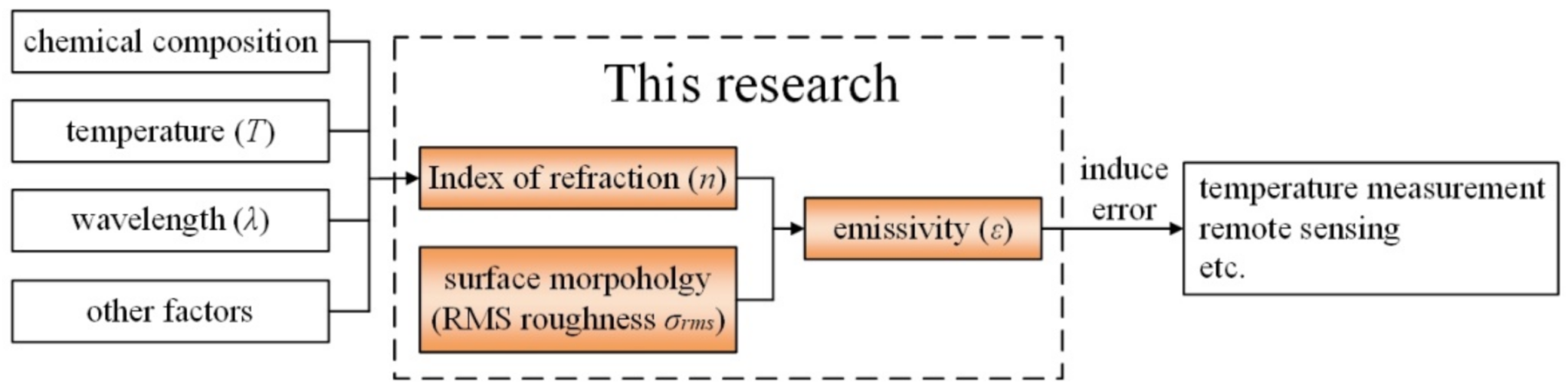
As a surface property parameter, the precise determination of emissivity is important in many fields, including infrared temperature measurement. Experimental studies have shown that the main factors affecting the emissivity of a given rough surface are the chemical composition [1], temperature [2,3,4], wavelength [2,3] and surface morphology [4,5], as shown in Figure 1. Closely related to the speed of light in the material, the index of refraction n depends mainly on the material, and is affected by temperature, wavelength and other factors. Surface morphology has an effect on reflection and shadowing, influencing the emissivity ε. In this paper, if not specifically indicated, the term emissivity refers to directional spectrum emissivity.

The indirect influences of temperature, wavelength and other factors on emissivity can be experimentally measured and are relatively clear. Studies on Pt-10Rh and SiC indicate that the emissivity of rough surface increases with the increase of temperature and the decrease of wavelength [6]. Similar phenomena are found in difficult-to-process materials including Inconel 718 and Ti6Al4V [3,7,8,9]. Other factors including chemical composition [1], heat treatment [2,3] and oxidation [10,11] may also have an effect on emissivity. The influence of chemical composition and heat treatment are combined in the influence of the index of refraction n. The oxide layers are neglectable if not specifically oxidized.

The influence of surface morphology is complicated and not yet well understood. It is found that coarsely sandblasted samples, compared with finely sandblasted samples, have higher total hemispherical emissivity at low temperature, but lower emissivity in high temperature [12]. It is also reported that differently processed surfaces with close surface roughness Ra may have very different emissivities [13]. Further information is needed to understand this ambiguity.

Theoretical modelling studies have been carried out to predict the emissivity of rough surfaces. This was predicted considering the shadowing effect [14]. The surface was however assumed as a grey body, which limits its application. The average probability that infrared radiation emitted hits the surface directly was calculated, and the influence of reflection on emissivity of rough surfaces was estimated by Wen and Mudawar [15]. Reflectivity of the rough surface is also affected by viewing angle. Thus, errors were introduced in applying the average probability. Emissivity model of rough surfaces considering shadowing effect and reflection was established [16], while the reflection was assumed no more than once. Emissivity model of sea surfaces have been carried out by Wu and Smith [17] and Li et al. [18,19,20,21] respectively. However, sea surfaces have certain patterns (perpendicular to the wind), and are composed merely by sea water. Their models lack in generality.

Despite this valuable work, due to the complexity of the emission processes, the influences of the index of refraction n and surface morphology on the directional emissivity ε are to be further studied, especially the influence of the index of refraction n. In this research, influences of the index of refraction n and root mean square (RMS) roughness σ_rms on emissivity ε are modeled, as shown in Figure 1. Geometric optics are assumed and a directional spectral emissivity prediction model based on the Gaussian random rough surface is briefly analyzed, as similar models have already been proposed and derived in other fields [18,22]. Then, a novel matrix method was introduced, and sectional Romberg integral is applied, to numerically solve the proposed model. Influences of the index of refraction n and the root mean square (RMS) roughness σ_rms on the directional emissivity ε are analyzed and discussed. It is found that emissivity of surfaces with lower σ_rms and higher n tends to have a peak in high viewing angles. On the contrary, the emissivity of surfaces with higher σ_rms and lower n tends to have a peak in low viewing angles. Finally, experimental verification based on IR temperature measurement of an Inconel 718 machined surface is carried out.

2. Methodology

In the model part, the surface is assumed to be Gaussian, and limited to the area of geometrical optics (GO). According to the number of reflecting processes involved, the emissivity is divided into components. To contribute to one component, an infrared ray must experience processes including emission, shadowing and reflection. As the surface is random, each process can only be discussed statistically by a possibility density function, and each component calculated by integration. The expression of emissivity is derived by summarizing the components. In this part, it is noticed that the emission, shadowing and reflection processes have no inner connection, and can be expressed separately. Similar processes of different components share the same properties, and can be depicted by one formula.

The expression of emissivity is too complex to be solved analytically. In the numerical solution part, considering the discoveries above, a matrix method is designed. Emission, shadowing and reflection processes are represented and computed by matrixes. Nested loops are avoided and computational time is shortened.

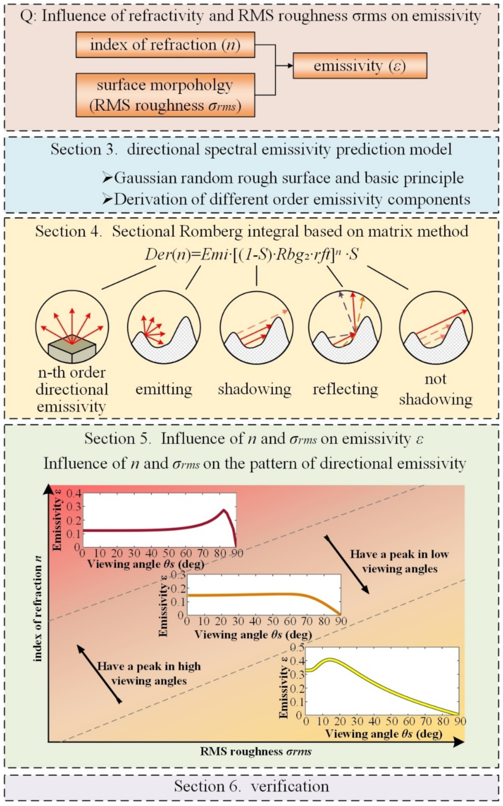
Experimental verification based on IR temperature measurement of an Inconel 718 machined surface is carried out. Temperature and emissive power are measured simultaneously to calculate the emissivity. Other experimental studies are also cited to further verify the model. The framework of this paper is displayed in Figure 2.

3. Modeling of Directional Emissivity of Rough Surfaces

3.1. Analysis of Emissivity of Rough Surfaces

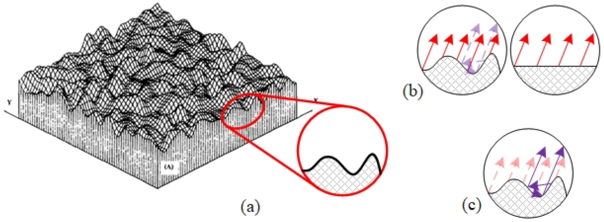
To predict the emissivity of rough surfaces, three-dimensional Gaussian random rough surface is assumed, as shown in Figure 3. The three-dimensional Gaussian random rough surface is generated by a stationary stochastic process, as expressed by Equation (1) [22]:

$$\langle \zeta (\mathit{r})\rangle =0$$

(1)

$$〈\zeta (\mathit{r})\zeta \left(\mathit{r}’\right)〉={\sigma }_{rms}^2\cdot e^{\frac{-{\left(x_1-x_2\right)}^2-{\left(y_1-y_2\right)}^2}{2{\sigma }_{rms}^2}}$$

(2)

where r is the position vector, and x, y, z are the coordinates of r. We have:

$$t_N\left(p,q,{\sigma }_{rms}\right)=\frac{1}{2\pi {\sigma }_{rms}^2}\cdot e^{\frac{-p^2-q^2}{2{\sigma }_{rms}^2}}$$

(3)

where p, q are the slopes of the surface in x, y direction, respectively. t_N (p, q, σ_rms) is the probability density function of p, q. The Gaussian random rough surfaces have the following characteristics:

• The surface is isotropic (and statistically symmetry);
• p and q are randomly distributed according to a Gaussian distribution;
• No correlation between p and q.

In this study, emissivity is defined as the emissive power of the rough surface compared with a black body, and geometric optics is assumed. According to Fresnel’s law and the reflection law:

$${\epsilon }_F\left(n,{\theta }_s\right)=\left\{\begin{array}{ll}\frac{\sqrt{n^2-{\sin }^2\left({\theta }_s\right)}}{n^2\cos \left({\theta }_s\right)+\sqrt{n^2-{\sin }^2\left({\theta }_s\right)}}+\frac{\cos \left({\theta }_s\right)}{\cos \left({\theta }_s\right)+\sqrt{n^2-{\sin }^2\left({\theta }_s\right)}},\hfill & \tan {\theta }_s<n\hfill \\ \frac{n^2\cos \left({\theta }_s\right)}{n^2\cos \left({\theta }_s\right)+\sqrt{n^2-{\sin }^2\left({\theta }_s\right)}}+\frac{\cos \left({\theta }_s\right)}{\cos \left({\theta }_s\right)+\sqrt{n^2-{\sin }^2\left({\theta }_s\right)}},\hfill & \tan {\theta }_s\ge n\hfill \end{array}\right.$$

(4)

where ε_F is emissivity, n is the index of refraction, θ_S is the viewing angle.

The main phenomena in the emission process of rough surfaces are Fresnel’s law and reflection enhancement. Figure 3b shows that the smooth surface consists of many horizontal microelements, while the rough surface consists of elements with varied directions, each having different emissivity in the same direction. Reflection enhancement refers to the phenomenon whereby reflection induces higher emissivity near the normal direction in rough surfaces, as depicted in Figure 3c. Reflection enhancement may also cause lower emissivity in high viewing angles. Due to their combined effect, the influence of surface morphology is complicated and not yet well understood.

3.2. Modelling of Emissivity of Rough Surfaces

Directional spectral emissivity refers to the ability of measured surface to emit in a certain wavelength and direction compared with a black body. A statistical model is established to calculate the emissivity of rough surfaces.

Infrared radiation emitted by an element may leave the surface directly (zeroth-order), reflect once (first-order), twice (second-order), and so on. Considering that the correlation between emissivity and the emitted power is linear, the emissivity could be divided into different order components, and the components can be computed separately. Components of second order and above are called high-order components collectively, as presented in Equation (5):

$$\epsilon ={\displaystyle \sum _{i=0}^{\infty }{\epsilon }_i}$$

(5)

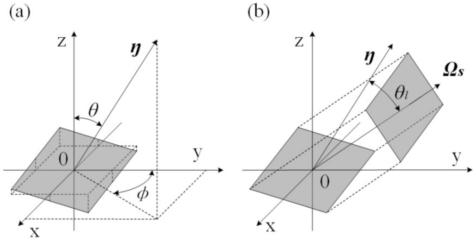
Zeroth-order component refers to emissivity related to infrared radiation that leaves the surface directly. To contribute to zeroth-order component, an infrared ray must be emitted, and not be blocked by another part of the surface. Different elements have different directions, and thus have different local viewing angle θ_l, as illustrated in Figure 4b. According to Equation (4), their local emissivities ε_l are not equal. The emitted radiation ray may also be blocked by another element, and the possibility is a function of its slope.

In Figure 4a:

$$\mathit{\eta }=\left(\frac{-p}{\sqrt{p^2+q^2+1}},\frac{-q}{\sqrt{p^2+q^2+1}},\frac{1}{\sqrt{p^2+q^2+1}}\right)$$

(6)

where η is the normal direction of the element. As shown in Figure 4b, projection of the element distorts depending on η and the viewing direction Ω_S. Thus, area projection coefficient A_p is:

$$A_p=\left\{\begin{array}{ll}{\mathit{\eta }}_{yoz}\cdot {\mathit{\Omega }}_s=\cos \left({\theta }_s\right)-q\sin \left({\theta }_s\right),\hfill & q<\cot \left({\theta }_s\right)\hfill \\ 0,\hfill & q\ge \cot \left({\theta }_s\right)\hfill \end{array}\right.$$

(7)

where η_yoz is the component of η in plane yoz.

$$t\left({\theta }_s,p,q,{\sigma }_{rms}\right)=\frac{A_p\cdot e^{\frac{-p-q}{2{\sigma }_{rms}^2}}}{{\displaystyle {\int }_{-\infty }^{\cot {\theta }_s}{\displaystyle {\int }_{-\infty }^{\infty }{A}_p}}\cdot e^{\frac{-p^2-q^2}{2{\sigma }_{rms}^2}}dpdq},\left(q<\cot {\theta }_s\right)$$

(8)

where t (θ_s, p, q, σ_rms) is the possibility that the slope of the emitting element is p, q. Smith’s shadowing function S(θ_s, σ_rms) [24,25] is the possibility that infrared radiation is not blocked. It has been reported [26,27] that correlation between elements is not significant and can be ignored. Smith’s shadowing function is estimated as Equation (9):

$$S\left({\theta }_s,{\sigma }_{rms}\right)==\left\{\begin{array}{cc}\frac{1}{\Lambda \left({\theta }_s,{\sigma }_{rms}\right)+1},& {\theta }_s<\frac{\pi }{2}\\ 0,& {\theta }_s\ge \frac{\pi }{2}\end{array}\right.$$

(9)

$$\Lambda \left({\theta }_s,{\sigma }_{rms}\right)=\frac{1}{2}\sqrt{\frac{2}{\pi }}\cdot \frac{{\sigma }_{rms}}{\cot {\theta }_s}{e}^{-\frac{{\cot }^2{\theta }_s}{2{\sigma }_{rms}}}-\mathrm{erfc}\left(\frac{\cot {\theta }_s}{\sqrt{2}{\sigma }_{rms}}\right)$$

(10)

$${\epsilon }_l\left(n,p,q,{\theta }_s\right)=\left\{\begin{array}{cc}\frac{\sqrt{n^2-{\sin }^2\left({\theta }_{sl}\right)}}{n^2\cos \left({\theta }_{sl}\right)+\sqrt{n^2-{\sin }^2\left({\theta }_{sl}\right)}}+\frac{\cos \left({\theta }_{sl}\right)}{\cos \left({\theta }_{sl}\right)+\sqrt{n^2-{\sin }^2\left({\theta }_{sl}\right)}},& \tan {\theta }_{sl}<n\\ \frac{n^2\cos \left({\theta }_{sl}\right)}{n^2\cos \left({\theta }_{sl}\right)+\sqrt{n^2-{\sin }^2\left({\theta }_{sl}\right)}}+\frac{\cos \left({\theta }_{sl}\right)}{\cos \left({\theta }_{sl}\right)+\sqrt{n^2-{\sin }^2\left({\theta }_{sl}\right)}},& \tan {\theta }_{sl}\ge n\end{array}\right.$$

(11)

$${\theta }_{sl}\left({\theta }_s,p,q\right)={\cos }^{-1}\left(\frac{\cos \left({\theta }_s\right)-q\sin \left({\theta }_s\right)}{\sqrt{1+p^2+q^2}}\right)$$

(12)

The zeroth-order component is,

$${\epsilon }_0={\displaystyle {\int }_{-\infty }^{\cot {\theta }_s}{\displaystyle {\int }_{-\infty }^{\infty }t}}\left({\theta }_s,p,q,{\sigma }_{rms}\right)S\left({\theta }_s,{\sigma }_{rms}\right){\epsilon }_l\left(n,p,q,{\theta }_s\right)dpdq$$

(13)

In Equation (13), we note that S(θ_s, σ_rms) is not a function of p, q. The integration part depicts the emission process, while S(θ_s, σ_rms) stands for not being blocked.

The first-order component refers to emissivity related to infrared radiation that reflects once before leaving the surface. To contribute to a zeroth-order component, an infrared ray must be emitted, hit another part of the surface, be reflected, and not hit the surface again. The process could be divided into two parts: emission and blocking, reflecion and exiting. Figure 5 shows that the infrared radiation emitted by the first element hits the second element in direction Ω₁, and the reflected beam leaves the surface in direction Ω_S. By applying the local coordinate system x’y’z’, the emission process is similar to the zeroth-order component.

According to the reflection law [28]:

$$\eta =\frac{{\mathit{\Omega }}_s-{\mathit{\Omega }}_1}{\left|{\mathit{\Omega }}_s-{\mathit{\Omega }}_1\right|}$$

(14)

which is:

$$p=\frac{\sin {\theta }_1\sin {\varphi }_1}{\cos {\theta }_s-\cos {\theta }_1}$$

(15)

$$q=\frac{\sin {\theta }_1\cos {\varphi }_1-\sin {\theta }_s}{\cos {\theta }_s-\cos {\theta }_1}$$

(16)

By substituting Equations (11) and (12) into Equations (7) and (8), $t\left({\theta }_1,p,q,{\sigma }_{rms}\right)$ and ${\epsilon }_l\left(n,p,q,{\theta }_s\right)$ could be expressed as $t\left({\theta }_s,{\theta }_1,{\varphi }_1,{\sigma }_{rms}\right)$ and ${\epsilon }_l\left(n,{\theta }_1,{\varphi }_1,{\theta }_s\right)$. According to Kirchhoff’s law we have [28]:

$$\rho =1-\alpha =1-{\epsilon }_l$$

(17)

where α, ρ are the absorptivity and reflectivity, respectively. Noting that Gaussian random rough surface is isotropic and statistically symmetry, we have:

$${\epsilon }_1={\displaystyle {\int }_0^{2\pi }{\displaystyle {\int }_0^{\pi -{\theta }_s}i\left({\theta }_1,{\sigma }_{rms}\right)t\left({\theta }_s,{\theta }_1,{\varphi }_1,{\sigma }_{rms}\right)S\left({\theta }_s,{\sigma }_{rms}\right)\left[1-{\epsilon }_l\left(n,{\theta }_1,{\varphi }_1,{\theta }_s\right)\right]\cdot \sin {\theta }_{1}d{\theta }_{1}d{\varphi }_1}}$$

(18)

$$i\left({\theta }_1,{\sigma }_{rms}\right)={\displaystyle {\int }_{-\infty }^{\cot {\theta }_1}{\displaystyle {\int }_{-\infty }^{\infty }t}}\left({\theta }_1,p_1,q_1,{\sigma }_{rms}\right)\left[1-S\left({\theta }_1,{\sigma }_{rms}\right)\right]{\epsilon }_l\left(n,{\theta }_1,{\varphi }_1,{\theta }_s\right)d{p}_{1}d{q}_1$$

(19)

where Equation (18) refers to the reflection process, and Equation (19) refers to the emitting process. Noting that S(θ_s, σ_rms) is not a function of p, q. Equation (13b) is mainly about emission and blocking, while Equation (18) is about reflection and exiting. In Equation (19), the integration part depicts the emission process, while [1 − S(θ_s, σ_rms)] stands for blocking, which is similar to Equation (13). In Equation (19), S(θ_s, σ_rms) stands for exiting, and the rest for reflection.

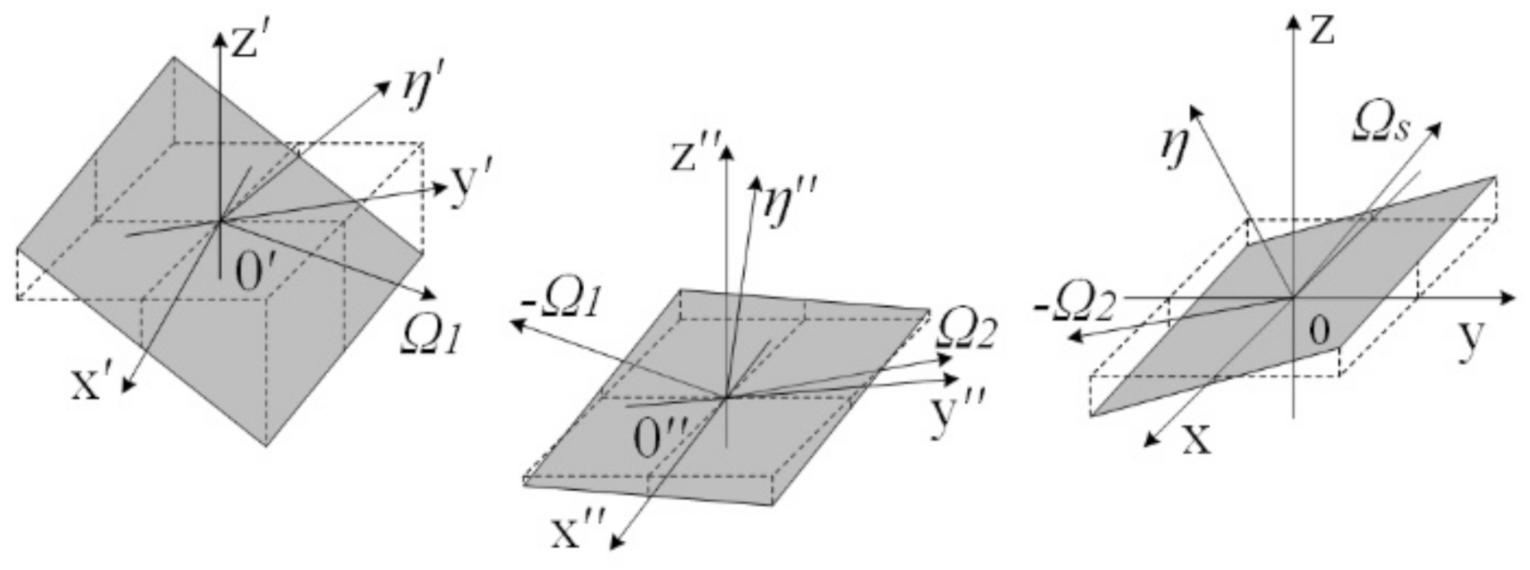
As shown in Figure 6, second-order component refers to emissivity related to infrared radiation that reflects twice before leaving the surface. By applying a local coordinate system to the first element and the second element, we have:

$${\epsilon }_2={\displaystyle {\int }_0^{2\pi }{\displaystyle {\int }_0^{\pi -{\theta }_s}{i}_2}}\left({\theta }_2,{\sigma }_{rms}\right)t\left({\theta }_s,{\theta }_2,{\varphi }_2,{\sigma }_{rms}\right)S\left({\theta }_s,{\sigma }_{rms}\right)\left[1-{\epsilon }_l\left(n,{\theta }_2,{\varphi }_1\right)\right]\cdot \sin {\theta }_{2}d{\theta }_{2}d{\varphi }_2$$

(20)

$$\begin{array}{cc}\hfill i_2\left({\theta }_2,{\sigma }_{rms}\right)={\int }_{-\infty }^{\cot {\theta }_2}& {\displaystyle {\int }_{-\infty }^{\infty }{i}_1}\left({\theta }_1,{\sigma }_{rms}\right)t\left({\theta }_s,{\theta }_1,{\varphi }_1,{\sigma }_{rms}\right)\hfill \\ & \left[1-S\left({\theta }_s,{\sigma }_{rms}\right)\right]\left[1-{\epsilon }_l\left(n,{\theta }_1,{\varphi }_1\right)\right]\cdot \sin {\theta }_{1}d{\theta }_{1}d{\varphi }_1\hfill \end{array}$$

(21)

$$i_1\left({\theta }_1,{\sigma }_{rms}\right)={\displaystyle {\int }_{-\infty }^{\cot {\theta }_1}{\displaystyle {\int }_{-\infty }^{\infty }t}}\left({\theta }_1,p_1,q_1,{\sigma }_{rms}\right)\left[1-s\left({\theta }_1,{\sigma }_{rms}\right)\right]{\epsilon }_l\left(n,p_1,q_1\right)d{p}_{1}d{q}_1$$

(22)

Third order component and above are modeled similarly. We note that emissivity is not a function of φ and the model is symmetrical.

4. Numerical Solution Based on a Matrix Method

The directional spectral emissivity of the rough surfaces is too complex to be solved analytically. Generally, multiple integrals are computed by nested loops, and the operation period of nested loops increases exponentially with multiplicity. In this section, a novel matrix method is introduced, and sectional Romberg integral is applied to obtain numerical solutions quickly and precisely.

As shown in Section 3.2, high-order components are related to two basic process, emission and refraction. As mentioned in Section 3.1, a Gaussian random rough surface is isotropic (and symmetrical), and no correlation between p and q is assumed. From another point of view, the optics processes involved are emission, reflection and shadowing. Thus, these processes can be represented by irrelevant matrixes. The numerical integration could be obtained by multiplying matrixes, which is much quicker than nested loops. We define:

$$Der(n)=Emi\cdot {\left[(1-S)\cdot Rb{g}_2\cdot rft\right]}^n$$

(23)

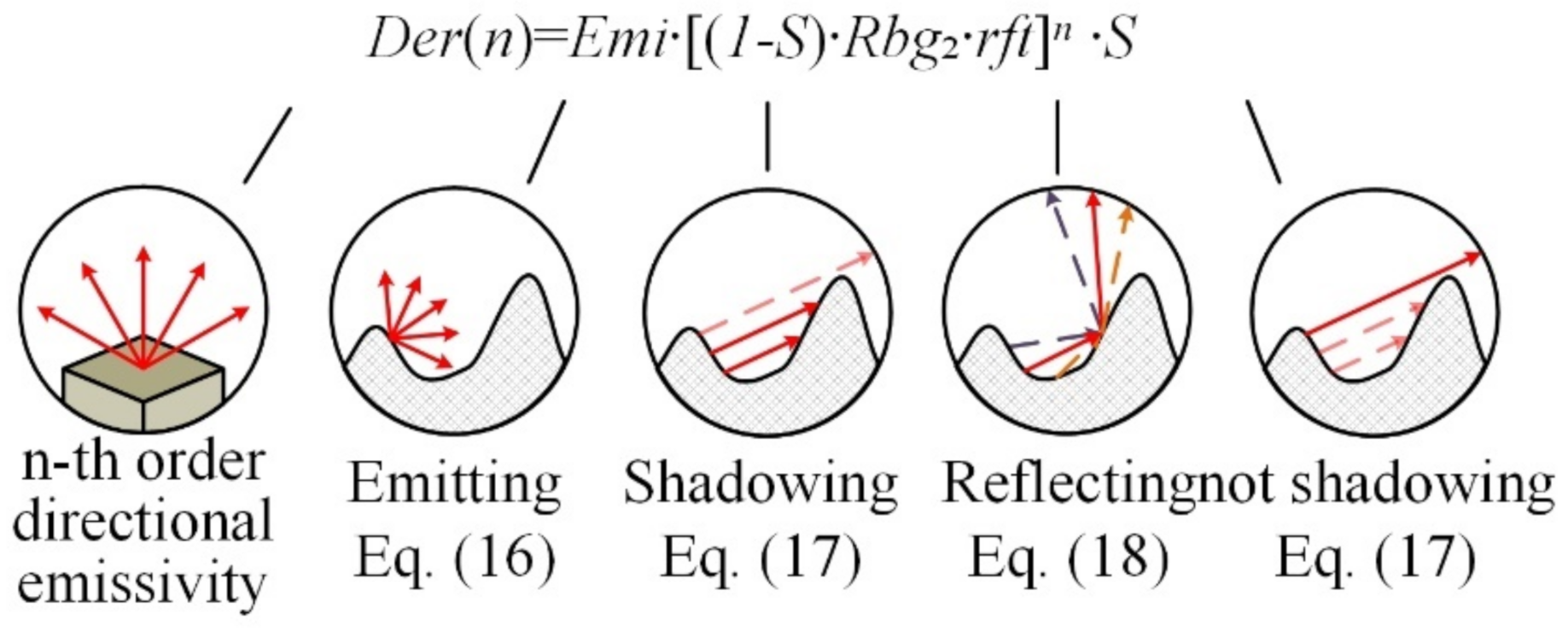
where Der(n) is the n-th order emissivity in the viewing angle ${\theta }_{s_k}$. Emi is the emission matrix. S is the shadowing matrix. Rbg₂ is the Romberg matrix. Definitions of Rbg₂ and theoretical verification of the matrix method are presented in Appendix A. rft is the reflection matrix. This gives:

$$Emi=\left[\begin{array}{ccccc}em{i}_1& em{i}_2& em{i}_3& \dots & em{i}_{97}\end{array}\right]$$

(24)

$$em{i}_k={\displaystyle {\int }_{-\infty }^{\cot {\theta }_{s_k}}{\displaystyle {\int }_{-\infty }^{\infty }t}}\left({\theta }_{s_k},p,q,{\sigma }_{rms}\right){\epsilon }_F(n,p,q)dpdq$$

(25)

where ${\theta }_{s_k}$ are, respectively.

$$S=\left[S\left({\theta }_{s_1},{\sigma }_{rms}\right)\hspace{1em}S\left({\theta }_{s_2},{\sigma }_{rms}\right)\hspace{1em}S\left({\theta }_3,{\sigma }_{rms}\right)\hspace{1em}\dots \hspace{1em}S\left({\theta }_{s_{97}},{\sigma }_{rms}\right)\right]$$

(26)

$$rft=\left[\begin{array}{cccc}rf{t}_{11}& rf{t}_{12}& \dots & rf{t}_{197}\\ rf{t}_{21}& rf{t}_{22}& \dots & rf{t}_{2}97\\ ⋮& ⋮& \ddots & ⋮\\ rf{t}_{971}& rf{t}_{972}& \dots & rf{t}_{9797}\end{array}\right]$$

(27)

$$rf{t}_{lk}=\left(\pi -{\theta }_{s_k}\right)\cdot {\displaystyle {\int }_0^{2\pi }t}\left({\theta }_{s_k},{\theta }_l,\varphi ,{\sigma }_{rms}\right)\left[1-{\epsilon }_l\left(n,{\theta }_l,\varphi \right)\right]\cdot \sin {\theta }_{l}d\varphi$$

(28)

From the viewpoint of optics, as sketched in Figure 7, Emi, (1 − S), Rbg₂, rft are defined, representing the emission, shadowing, reflection and leaving processes, respectively. emi_k is the average emissivity of a random element in direction θ_K. Elements of (1 − S) are the possibility that a ray in direction θ_K hits the surface again. Rbg₂ is a constant matrix introduced by Romberg integration. Rft_lk is the average energy reflected to direction θ_K when a ray from direction θ_l hits a random element. Thus, the infrared rays are traced statistically by a matrix method.

Multiple integrations are generally computed by nested loops, in which t (θ_S, p, q, σ_rms) and ε_F (n, p, q) must be calculated repeatedly in every step of every integration. Thus, computational time increases exponentially with the order n. In matrix method, they are computed only in obtaining the matrixes. Therefore, the computational time hardly increases when n > 0. The amount of calculation is presented in

Table 1. How many times t (θ_S, p, q, σ_rms) and ε_F (n, p, q) are calculated in nested loops and matrix method.

Approach	ε0	ε1	ε2	ε3	ε4
nested loops	2.62∙105 a	3.82∙109	8.00∙1012	1.64∙1016	3.36∙1019
matrix method	2.62∙105	4.77∙108	4.77∙108	4.77∙108	4.77∙108

^a The results are counted by MATLAB program, when h_θ = 1/128 ≈ 0.008, h_p = π/32 ≈ 0.1, θ_S = 20°, σ_rms = 0.33.

.

Table 2. The influence of n and σ_rms on estimated error.

Index of Refraction n	RMS Roughness σrms
	0	0.2	0.5	1	2
1	2∙10−9 a	3.55∙10−5	8.00∙10−5	6.23∙10−6	5.65∙10−6
2	3.18∙10−6	1.22∙10−4	2.33∙10−4	1.80∙10−4	2.78∙10−4
4	1.86∙10−6	2.43∙10−4	1.65∙10−4	1.15∙10−4	1.21∙10−4
8	1.38∙10−6	4.13∙10−4	1.80∙10−4	2.10∙10−4	1.26∙10−4
16	4.59∙10−6	2.75∙10−4	3.10∙10−4	3.54∙10−4	3.34∙10−4

^a Accuracy of the PC in this research is 2⁻³⁰ (about 10⁻⁹). Thus, this data has only one significant figure.

illustrates that the estimated error of the matrix method is acceptable. Estimation of the error is summarized in Appendix A.

5. Results and Discussion

The effects of the index of refraction n and the RMS roughness σ_rms on the emissivity ε are discussed by setting different parameters. The numerical integral was carried out with the MATLAB R2018a program, using a personal computer running with an Intel Core I7-4720HQ, 3.6 GHz. CPU. In industry, n is mostly between 2 and 16, σ_rms is mostly under 1. The values of n and σ_rms is chosen inside this range by proportional sequences, to cover the majority of rough surfaces encountered in industry.

5.1. Pattern of Different Components

The patterns of different components are discussed. Figure 8 displays that higher order components are considerably smaller in scale. The proportion of higher order components increases with increasing σ_rms. The components of first order and above are almost 0 when the surface is smooth, and consists of only about 20% when the surface is relatively rough.

5.2. Effects of the Index of Refraction n on Emissivity ε

The index of refraction n depends on the chemical composition of the surface and varies with wavelength and temperature [28].

When the RMS roughness σ_rms is relatively high, ε would be dominated by σ_rms, which is to be discussed in Section 5.3. When σ_rms is relatively low, p, q converge to zero, and the surface would be too smooth for an infrared ray emitted to hit the surface again. Thus, ε depends mainly on ε₀, and ε_l ≈ ε_F. Equation (6) could be transformed into the following form:

$${\epsilon }_0=S\left({\theta }_s,{\sigma }_{rms}\right)emi\left({\theta }_s,n,{\sigma }_{rms}\right)$$

(29)

$$emi\left({\theta }_s,n,{\sigma }_{rms}\right)={\displaystyle {\int }_{-\infty }^{\cot {\theta }_s}{\displaystyle {\int }_{-\infty }^{\infty }t}}\left({\theta }_s,p,q,{\sigma }_{rms}\right){\epsilon }_l\left(n,p,q,{\theta }_s\right)dpdq$$

(30)

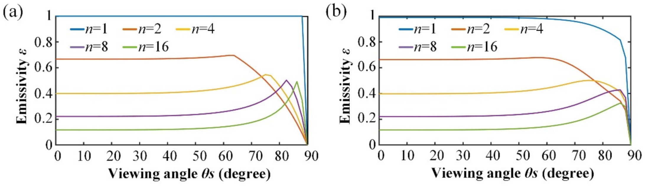
The patterns shown in Figure 9b are reported in experimental studies [14,29]. It is shown in Figure 9 that ε_F and ε have similar patterns. Obviously, n affects ε_l (ε_l ≈ ε_F), and thus have an effect on ε. In another word, n influences ε_l by influencing the emission characteristics of the elements. emi (θ_S, n, σ_rms) is the same function that stands for the emission process mentioned in Section 4. In Equation (4), it can be analytically demonstrated that the extreme point is the polarizing angle, which is really interesting. Such a phenomenon could be valuable for further research.

5.3. Effects of RMS Roughness σ_rms on Emissivity ε

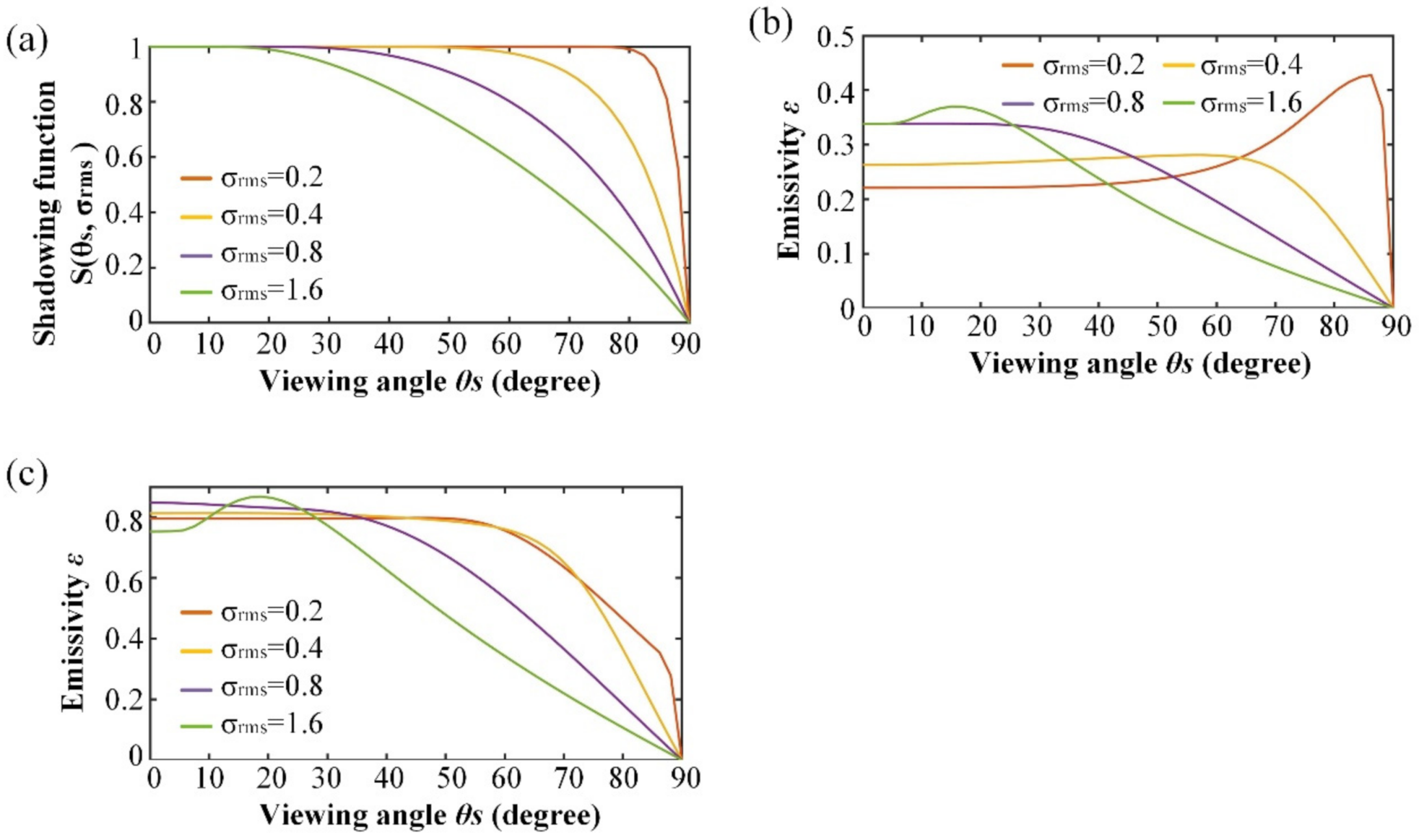
Referring to the root mean square of the slope of the surface elements, RMS roughness σ_rms is a surface integrity parameter. According to Equations (29) and (30), σ_rms affects both S (θ_S, σ_rms) and emi (θ_S, n, σ_rms). That is, σ_rms effects both of emission and shadowing. ε decreases with increasing σ_rms in high viewing angle, increases with increasing σ_rms in middle viewing angle, and first increases then decreases with increasing σ_rms in low viewing angle (near normal direction). Surfaces with very high σ_rms may have a peak in low viewing angle. It should be noted that high, middle and low here are a relative concept. As higher order components are relatively small, reflection is not discussed in details here.

As shown in Figure 10, on the one hand, the shadowing effect becomes more notable with increasing σ_rms. Figure 10a shows that S (θ_S, σ_rms) decreases with increasing σ_rms in high viewing angle. Thus, ε decreases with increasing σ_rms in high viewing angle. On the other hand, these blocked infrared rays are redistributed in all directions, including middle viewing angles. Thus, ε increases with increasing σ_rms in middle viewing angle.

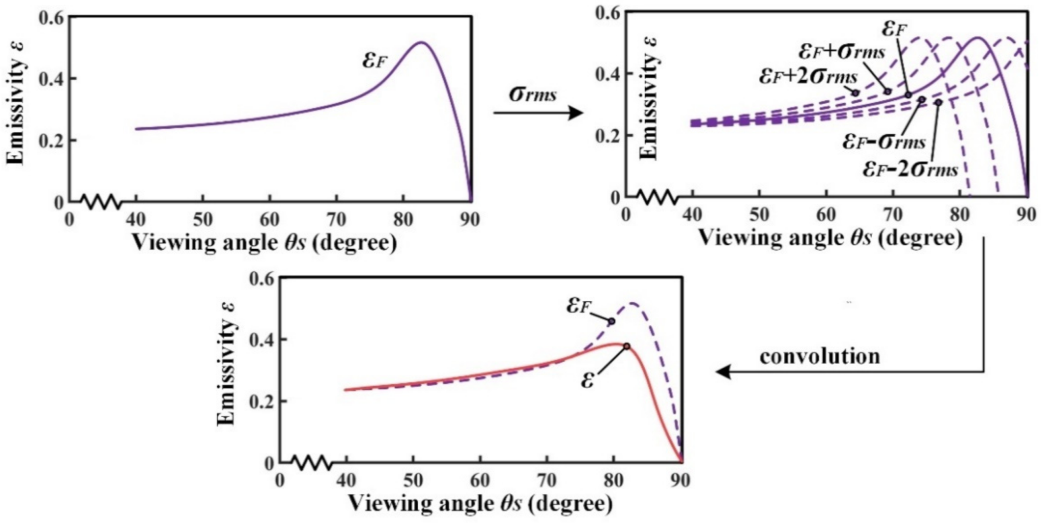
On the other hand, emi (θ_S, n, σ_rms) varies with increasing σ_rms. Local emissivity of the elements ε_F (θ_S, n) are not a function of σ_rms, but the distribution of the elements can be influenced by σ_rms. Thus, σ_rms have an effect on the emissivity ε. As shown in Figure 11, emi (θ_S, n, σ_rms) could be considered as a convolution of ε_F (θ_S, n). Thus, the curve is flattened and the emissivity decreases with increasing σ_rms in high viewing angles, and increases with increasing σ_rms in middle viewing angles. The emissivity ε is dominated by σ_rms, and n have little effect on ε, as mentioned in Section 5.2. Similar patterns are reported experimentally [13,20].

Near normal direction, the effect of σ_rms in middle viewing angle still works, and ε increase with increasing σ_rms firstly. While σ_rms is very high, 2∙σ_rms may proceed the polarizing angle, where ε_F starts to decrease with increasing θ_S. Thus, ε near normal direction may decrease with increasing σ_rms. Due to this phenomenon near normal direction, surfaces with very high σ_rms tend to have a peak in low viewing angles.

5.4. Combined Effect of n and σ_rms on ε

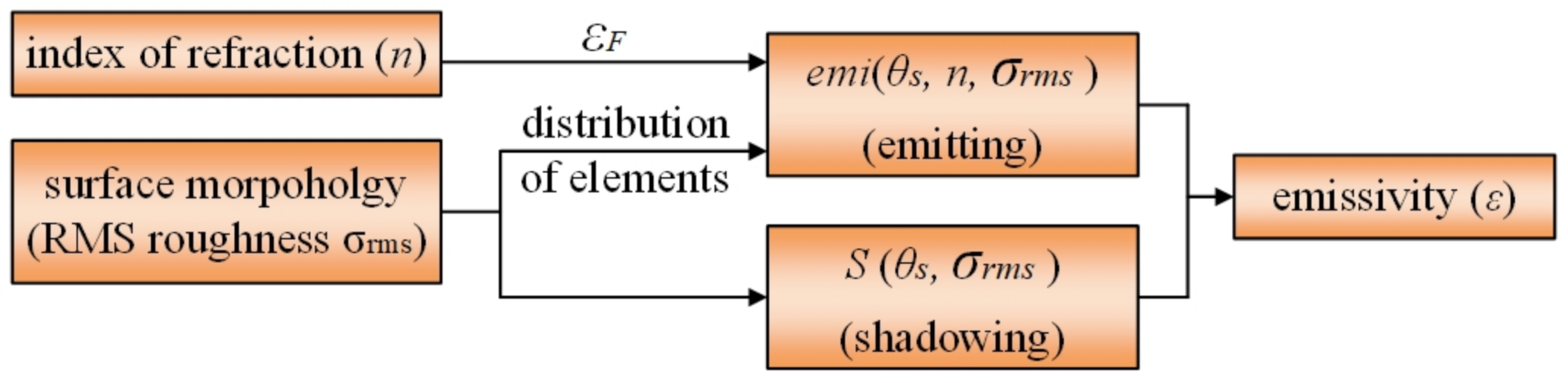
Influences of the index of refraction n and root mean square (RMS) roughness σ_rms on emissivity ε are discussed based on Section 5.2 and Section 5.3. n have an impact on emi (θ_S, n, σ_rms) by ε_F, and thus influences ε. σ_rms influences both emi (θ_S, n, σ_rms) and S (θ_S, σ_rms). In optics point of view, n influences primarily emission process, while σ_rms influences both emission and shadowing, as shown in Figure 12.

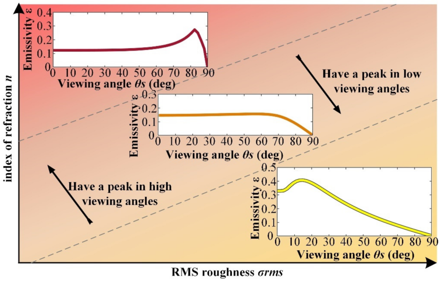
When σ_rms is relatively high, ε is dominated by σ_rms. It is found that ε decreases with increasing σ_rms in high viewing angle, increases with increasing σ_rms in middle viewing angle, and first increases then decreases with increasing σ_rms near normal direction. Therefore, surfaces with very high σ_rms may have a peak in low viewing angle. When σ_rms is relatively low, ε tend to decrease with increasing n, and have a steeper peak in high viewing angles. The extreme point is the Brewster’s angle, which increases with increasing n.

Summarizing the conclusions above, surfaces can be divided into three areas depending on index of refraction n and RMS roughness σ_rms. Surfaces with lower σ_rms and higher n tends to have a peak in high viewing angles [30,31,32]. On the contrary, surfaces with higher σ_rms and lower n tends to have a peak in low viewing angles. There is an intermediate region between the two areas [29,32], as shown in Figure 13.

6. Verification by Simulated Experiment

According to Plunk’s law:

$$E(\lambda ,T)=\epsilon \frac{C_1{\lambda }^{-5}}{e^{\frac{C_2}{\lambda T}}-1}$$

(31)

where C₁ ≈ 3.7418∙10⁻¹⁶ W∙m², C₂ ≈ 1.4388∙10⁻² m∙K.

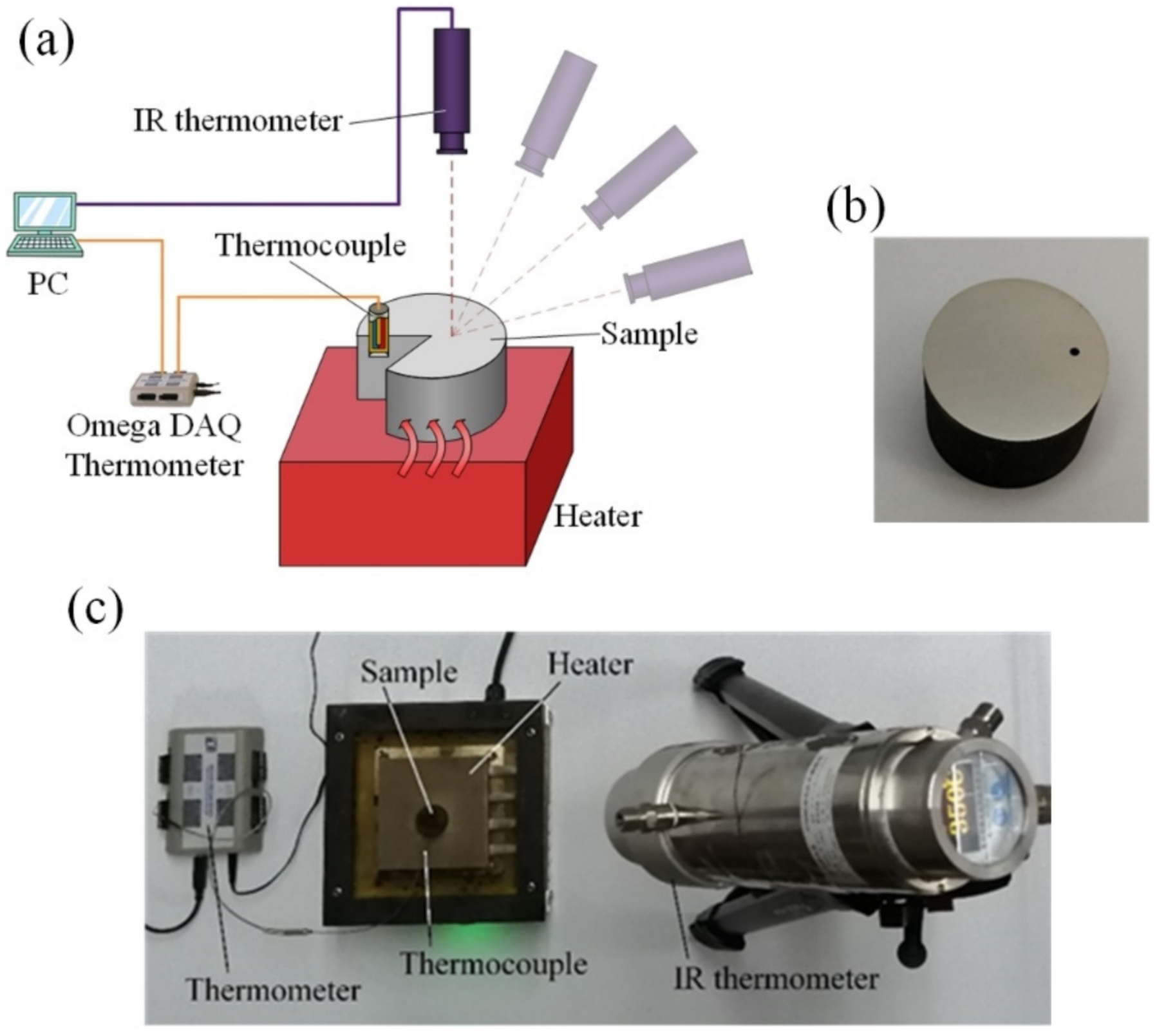
Thus, the emissivity of the surface could be calculated by measuring the temperature T and the emissive power E (λ, T). Figure 14a depicts the principle of the proposed verification experiment. The temperature T of the sample is measured by thermocouples. The emissive powe E (λ, T) is measured by an IR thermometer from different directions. All data is imported to a personal computer, by which the emissivity ε is calculated according to Equation (31). All samples are heated to one same temperature (900 K), in order to minimize the error.

As shown in Figure 14b, the samples introduced are polished Inconel 718 columns, ϕ 27 × 18 mm, with a blind hole drilled to place the thermocouple. Inconel 718 is a difficult-to-process material. The surface roughness of the samples were Ra 0.17 ± 0.009 μm, and the RMS roughness were 1.16 ± 0.05. State and properties of the sample were referred in [33]. As shown in Figure 14c, the temperature values of the samples were measured by a DAQ-2401 thermometer (OMEGA, city, state abbrev if USA, country) equipped with a type-K thermocouple.

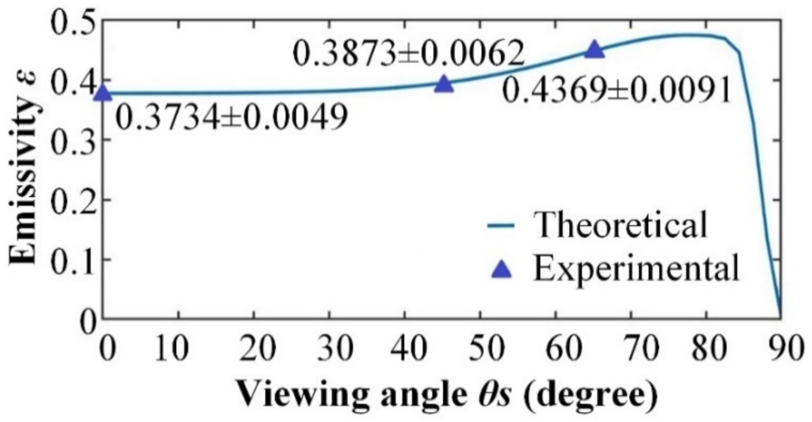
The emissive power E (λ, T) was measured by the IR thermometer. The wavelength of the IR thermometer is 1.7 μm. Further information was reported by Zhao [34] et al. The upper surface of the sample was heated to 900 K to minimum the environmental interference. Five points in one sample are chosen for each group in the experimental study. As shown in Figure 15, the experimental results match well with the model.

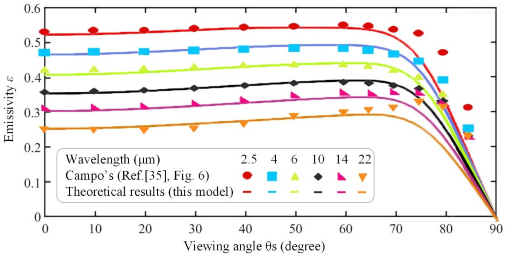
Sandblasted surfaces have similar pattern with Gaussian random rough surface. Emissivity of Inconel 718 sandblasted surfaces were reported by Campo [35] et al. Figure 16 shows that the experimental results match well with the theoretical results. Deviations at higher viewing angles might due to diffraction.

7. Conclusions

In this research, a theoretical model considering the index of refraction n and the root mean square (RMS) roughness σ_rms is established out to predict the emissivity ε of rough surfaces. The directional spectral emissivity prediction model based on the Gaussian random rough surface is proposed. Then, the sectional Romberg integration based on a novel matrix method is applied to numerically solve the proposed model. Influences of the index of refraction n and the RMS roughness σ_rms on the emissivity ε are analyzed and discussed. Experimental verification is carried out with Inconel 718 samples. In this research, diffraction is neglected, and the differences between real [36] and Gaussian rough surface are also neglected. Their potential effects on emissivity are to be further researched. The main conclusions drawn from this work are as follows:

(1)

A directional spectral emissivity prediction model of rough surfaces is established considering the shadowing effect and the reflection enhancement. Sectional Romberg integration based on a novel matrix method is applied to numerically solve the proposed model and is theoretically verified. The computational time of the matrix method is compared with that of the traditional method. Errors induced in the matrix method are estimated.

(2)

The influence of the index of refraction n and RMS roughness σ_rms on the emissivity ε is discussed according to the model. It is found that higher order components are smaller in scale and their energy is more concentrated near the normal direction.

(3)

n influences ε by influencing ε_F (or from an optics point of view, the emission process). When σ_rms is relatively low, ε tends to decrease with increasing n, and have a steeper peak in high viewing angles. The extreme point is the Brewster’s angle, which increases with increasing n. When the RMS roughness σ_rms is relatively high, ε would be dominated by σ_rms, and influence of n would be quenched.

(4)

σ_rms influences both S (θ_S, σ_rms) and emi (θ_S, n, σ_rms) (both emitting and shadowing). That is, σ_rms effects both of emitting and shadowing. ε decreases with increasing σ_rms in high viewing angle, increases with increasing σ_rms in middle viewing angle, and first increases then decreases with increasing σ_rms near normal direction. Surfaces with very high σ_rms may have a peak in low viewing angle.

(5)

Surface with lower σ_rms and higher n, due to Fresnel’s law, tends to have a peak in high viewing angles. On the contrary, surface with higher σ_rms and lower n, mainly due to reflection enhancement, tends to have a peak in low viewing angles. In the intermediate region, due to their combined effect, the emissivity has no recognizable peak and decreases with increasing viewing angle.

References

- Alaruri, S.; Bianchini, L.; Brewington, A. Effective spectral emissivity measurements of superalloys and YSZ thermal barrier coating at high temperatures using a 1.6 μm single wavelength pyrometer. Opt. Lasers Eng. 1998, 30, 77–91. [Google Scholar] [CrossRef]
- Kong, B.; Li, T.; Eri, Q. Normal spectral emissivity measurement on five aeronautical alloys. J. Alloys Compd. 2017, 703, 125–138. [Google Scholar] [CrossRef]
- González-Fernández, L.; Risueño, E.; Pérez-Sáez, R.B.; Tello, M.J. Infrared normal spectral emissivity of Ti-6Al-4V alloy in the 500–1150 K temperature range. J. Alloys Compd. 2012, 541, 144–149. [Google Scholar] [CrossRef]
- Tanda, G.; Misale, M. Measurement of total hemispherical emittance and specific heat of aluminum and inconel 718 by a calorimetric technique. J. Heat Transf. 2006, 128, 302–306. [Google Scholar] [CrossRef]
- Keller, B.P.; Nelson, S.E.; Walton, K.L.; Ghosh, T.K.; Tompson, R.V.; Loyalka, S.K. Total hemispherical emissivity of inconel 718. Nucl. Eng. Des. 2015, 287, 11–18. [Google Scholar] [CrossRef] [Green Version]
- Cagran, C.P.; Hanssen, L.M.; Noorma, M.; Gura, A.V.; Mekhontsev, S.N. Temperature-resolved infrared spectral emissivity of SiC and Pt-10Rh for temperatures up to 900 °C. Int. J. Thermophys. 2007, 28, 581–597. [Google Scholar] [CrossRef]
- Abbott, W.; Cook, C.R.; Garfield, G.; Barice, W.J. Titanium and Titanium Alloys; Matthew, J.D., Ed.; American Society for Metals: Geauga County, OH, USA, 1982. [Google Scholar]
- Xu, D.; Wang, Y.; Xiong, B.; Li, T. MEMS-based thermoelectric infrared sensors: A review. Front. Mech. Eng. 2017, 12, 557–566. [Google Scholar] [CrossRef]
- Ezugwu, E.O.; Wang, Z.M.; Machado, A.R. The machinability of nickel-based alloys: A review. J. Mater. Process. Technol. 1998, 86, 1–16. [Google Scholar] [CrossRef]
- González de Arrieta, I.; González-Fernández, L.; Risueño, E.; Echániz, T.; Tello, M.J. Isothermal oxidation kinetics of nitrided Ti-6Al-4V studied by infrared emissivity. Corros. Sci. 2020, 173, 108723. [Google Scholar] [CrossRef]
- Qi, J.; Eri, Q.; Kong, B.; Zhang, Y. The radiative characteristics of inconel 718 superalloy after thermal oxidation. J. Alloys Compd. 2020, 156414. [Google Scholar] [CrossRef]
- Frolec, J.; Králík, T.; Musilová, V.; Hanzelka, P.; Srnka, A.; Jelínek, J. A database of metallic materials emissivities and absorptivities for cryogenics. Cryogenics 2019, 97, 85–99. [Google Scholar] [CrossRef]
- Sabuga, W.; Todtenhaupt, R. Effect of Roughness on the Emissivity of the Precious Metals Silver, Gold, Palladium, Platinum, Rhodium, and Iridium. High Temp. High Press. 2001, 33, 261–269. [Google Scholar] [CrossRef]
- Rubanenko, L.; Schorghofer, N.; Greenhagen, B.T.; Paige, D.A. Equilibrium temperatures and directional emissivity of sunlit airless surfaces with applications to the moon. J. Geophys. Res. Planets 2020, 125. [Google Scholar] [CrossRef]
- Wen, C.-D.; Mudawar, I. Modeling the effects of surface roughness on the emissivity of aluminum alloys. Int. J. Heat Mass Transf. 2006, 49, 4279–4289. [Google Scholar] [CrossRef]
- Chen, K.S.; Wu, T.D.; Tsang, L.; Li, Q.; Shi, J.; Fung, A.K. Emission of rough surfaces calculated by the integral equation method with comparison to three-dimensional moment method simulations. IEEE Trans. Geosci. Remote Sens. 2003, 41, 90–101. [Google Scholar] [CrossRef]
- Wu, X.; Smith, W.L. Emissivity of rough sea surface for 8–13 μm: Modeling and verification. Appl. Opt. 1997, 36, 2609–2619. [Google Scholar] [CrossRef] [PubMed]
- Li, H.; Pinel, N.; Bourlier, C. Polarized infrared reflectivity of 2D sea surfaces with two surface reflections. Remote Sens. Environ. 2014, 147, 145–155. [Google Scholar] [CrossRef]
- Li, H.; Pinel, N.; Bourlier, C. Polarized infrared reflectivity of one-dimensional gaussian sea surfaces with surface reflections. Appl. Opt. 2013, 52, 6100–6111. [Google Scholar] [CrossRef]
- Li, H.; Pinel, N.; Bourlier, C. A monostatic illumination function with surface reflections from one-dimensional rough surfaces. Waves Random Complex Media 2011, 21, 105–134. [Google Scholar] [CrossRef]
- Li, H.; Pinel, N.; Bourlier, C. Polarized infrared emissivity of 2D sea surfaces with one surface reflection. Remote Sens. Environ. 2012, 124, 299–309. [Google Scholar] [CrossRef]
- Tang, K.; Buckius, R.O. A statistical model of wave scattering from random rough surfaces. Int. J. Heat Mass Transf. 2001, 44, 4059–4073. [Google Scholar] [CrossRef]
- Hu, Y.Z.; Tonder, K. Simulation of 3D random rough surface by 2D digital filter and fourier analysis. Int. J. Mach. Tools Manuf. 1992, 32, 83–90. [Google Scholar] [CrossRef]
- Smith, B.G. Geometrical shadowing of a random rough surface. IEEE Trans. Antennas Propag. 1967, 15, 668–671. [Google Scholar] [CrossRef]
- Smith, B.G. Lunar surface roughness: Shadowing and thermal emission. J. Geophys. Res. 1967, 72, 4059–4067. [Google Scholar] [CrossRef] [Green Version]
- Bourlier, C.; Berginc, G.; Saillard, J. Monostatic and bistatic statistical shadowing functions from a one-dimensional stationary randomly rough surface according to the observation length: I. Single scattering. Waves Random Media 2002, 12, 145–173. [Google Scholar] [CrossRef]
- Yoshimori, K.; Itoh, K.; Ichioka, Y. Optical characteristics of a wind-roughened water surface: A two-dimensional theory. Appl. Opt. 1994, 34, 6236–6247. [Google Scholar] [CrossRef] [PubMed]
- Born, M. Principles of Optics: Electromagnetic Theory of Propagation, Interference, and Diffraction of Light, 6th ed.; Wolf, E., Ed.; Pergamon Press: Oxford, UK, 1980. [Google Scholar]
- Balat-Pichelin, M.; Bousquet, A. Total hemispherical emissivity of sintered SiC up to 1850 K in high vacuum and in air at different pressures. J. Eur. Ceram. Soc. 2018, 38, 3447–3456. [Google Scholar] [CrossRef]
- Brodu, E.; Balat-Pichelin, M.; Sans, J.L.; Kasper, J.C. Influence of roughness and composition on the total emissivity of tungsten, rhenium and tungsten-25% rhenium alloy at high temperature. J. Alloys Compd. 2014, 585, 510–517. [Google Scholar] [CrossRef]
- Tang, K.; Buckius, R.O. The geometric optics approximation for reflection from two-dimensional random rough surfaces. Int. J. Heat Mass Transf. 1998, 41, 2037–2047. [Google Scholar] [CrossRef]
- Brodu, E.; Balat-Pichelin, M.; Sans, J.L.; Freeman, M.D.; Kasper, J.C. Efficiency and behavior of textured high emissivity metallic coatings at high temperature. Mater. Des. 2015, 83, 85–94. [Google Scholar] [CrossRef]
- Zhao, J.; Liu, Z. Influences of coating thickness on cutting temperature for dry hard turning inconel 718 with PVD TiAlN coated carbide tools in initial tool wear stage. J. Manuf. Process. 2020, 56, 1155–1165. [Google Scholar] [CrossRef]
- Zhao, J.; Liu, Z.; Wang, B.; Hua, Y.; Wang, Q. Cutting temperature measurement using an improved two-color infrared thermometer in turning inconel 718 with whisker-reinforced ceramic tools. Ceram. Int. 2018, 44, 19002–19007. [Google Scholar] [CrossRef]
- Del Campo, L.; Pérez-Sáez, R.B.; González-Fernández, L.; Esquisabel, X.; Fernández, I.; González-Martín, P.; Tello, M.J. Emissivity measurements on aeronautical alloys. J. Alloys Compd. 2010, 489, 482–487. [Google Scholar] [CrossRef]
- Țălu, Ș. Micro and Nanoscale Characterization of Three Dimensional Surfaces: Basics and Applications; Napoca Star Publishing House: Cluj-Napoca, Romania, 2015. [Google Scholar]
Figure 1.
Factors affecting the emissivity ε of rough surfaces.
Figure 2.
The framework of this paper.
Figure 3.
Effect of surface morphology on emissivity. (a): Gaussian random rough surface (Ref. [23], Figure 2) (b): Fresnel’s law. (c): Reflection enhancement.
Figure 4.
Zeroth-order component (a): Element. (b): Projection of the element.
Figure 5.
First-order component.
Figure 6.
Second-order component.
Figure 7.
Matrix method, in the viewpoint of optics.
Figure 8.
Components of emissivity (a): n = 4, σrms = 0.3; (b): n = 4, σrms = 0.5; (c): n = 4, σrms = 1.
Figure 9.
Comparison of the emissivity of elements and surfaces (σrms = 0.1). (a): Effect of the index of refraction n on emissivity of the elements εF. (b): Effect of n on emissivity of the surface ε.
Figure 10.
Effect of RMS roughness σrms on emitting process. (a): Effect on shadowing function S (θS, σrms). (b): Effect on ε when n = 8. (c): Effect on ε when n = 1.5.
Figure 11.
Effect of RMS roughness σrms on emitting process and emissivity ε.
Figure 12.
Mechanism of the influence of the index of refraction n and RMS roughness σrms on emissivity ε.
Figure 13.
Influence of the index of refraction n and RMS roughness σrms on the pattern of emissivity.
Figure 14.
Experimental setup of IR temperature measurement. (a): Principle of the measurement. (b): The sample in Figure 14a. (c): The equipment and sample involved in Figure 14a.
Figure 15.
Comparison between experimental and theoretical results (index of refraction n = 4.34).
Figure 16.
Experimental and theoretical results of smooth surface (Where RMS roughness σrms = 0.35, index of refraction n = 2.85, 3.35, 4.0, 4.8, 5.8, 7.2, respectively).