Substructure Shake Table Testing of Frame Structure–Damper System Using Model-Based Integration Algorithms and Finite Element Method: Numerical Study

Abstract

Substructure shake table testing (SSTT) is an advanced experimental technique that is suitable for investigating the vibration control of secondary structure-type dampers such as tuned mass dampers (TMDs). The primary structure and damper are considered as analytical and experimental substructures, respectively. The analytical substructures of existing SSTTs have mostly been simplified as SDOF structures or shear-type structures, which is not realistic. A common trend is to simulate the analytical substructure via the finite element (FE) method. In this study, the control effects of four dampers, i.e., TMD, tuned liquid damper (TLD), particle damper (PD) and particle-tuned mass damper (PTMD), on a frame were examined by conducting virtual SSTTs. The frame was modeled through stiffness-based beam-column elements with fiber sections and was solved by a family of model-based integration algorithms. The influences of the auxiliary mass ratio, integration parameters, time step, and time delay on SSTT were investigated. The results indicate that the TLD had the best performance. In addition, SSTT using model-based integration algorithms can provide satisfactory results, even when the time step is relatively large. The effects of integration parameters and time delay are not significant.

1. Introduction

Substructure shake table testing (SSTT) is one of the most advanced experimental techniques in structural and earthquake engineering [1]. It combines the advantages of the real-time dynamic loading of a shake table and the substructure technique from hybrid simulation (HS) and real-time hybrid simulation (RTHS). The best use of SSTT is for investigating the vibration control effects of dampers, such as the classical TMDs and TLDs, and emerging dampers, such as particle dampers (PDs) [2] and particle-tuned mass dampers (PTMDs) [3]. These dampers can be regarded as secondary structures with respect to the primary structure. To conduct SSTT, the damper and the primary structure are taken as the experimental and analytical substructures, which are experimentally tested on the shake table and numerically simulated on a computer, respectively.

The shake table tests are generally used for obtaining the dynamic responses and dynamic characteristics of structures [4,5]. The conventional experimental method of investigating the control effects of dampers is to carry out shake table tests for complete structure–damper systems. For instance, Kang et al. [6] conducted a series of 1:30 scaled model shake table tests and numerical simulations for a coal-fired power plant equipped with a large mass ratio multiple-tuned mass damper (LMTMD), and found that the LMTMD is effective and robust in reducing structural dynamic responses. Wang et al. [7] evaluated the performance of a pendulum pounding-tuned mass damper (PPTMD) by carrying out a series of shake table tests. They reported that the inherent damping of the primary structure decreases the control efficiency of the PPTMD. Zhao et al. [8] conducted shake table tests on a 1:8 scaled transmission tower equipped with and without TMDs, and found that the TMD’s control performance is related to earthquake type and excitation intensity. Vafaei et al. [9] proposed a modified-tuned liquid damper (MTLD) to attenuate multiple mode vibration. The effectiveness of the MTLD was demonstrated by several shake table tests on a scaled three-story structure with and without an MTLD. Lu et al. [3] explored the damping performance of a PTMD by comparing the shake table results of a scaled five-story steel frame with and without a PTMD. Based on the shake table tests, they conducted comprehensive parametric analyses on the reduction effects of PTMD, including the auxiliary mass ratio, gap clearance, and the mass ratio of particles to the total auxiliary mass. Shen et al. [10] investigated the influence of a double-layer-tuned particle damper (DTPD) on the seismic performance of super high-rise structures by conducting a series of 1:20 scaled model shake table tests on high-rise structures with and without DTPDs. They concluded that the effectiveness of the DTPD is closely related to the ground motion.

Compared with the conventional shake table tests for a complete structural system, one of the notable advantages of SSTTs is that any size effect of the specimen can be reduced. SSTT has also been applied to structure–damper systems. For instance, numerous researchers [11,12,13,14] investigated the performance of TLDs in controlling the seismic response of structures using a SSTT. Fu et al. [15,16] recently conducted the first SSTT of a single degree-of-freedom (SDOF)-PD system and compared the vibration control effects of TLDs and PDs based on the experimental results of a series of SSTTs. It should be noted, however, that the analytical substructures in most existing studies were optimized to be SDOF structures or shear-type structures with few DOFs. This is because these structures do not require considerable computational time to solve their equations of motion (EOMs). However, oversimplification of the analytical substructure may hinder the application of SSTT in real engineering practice. Therefore, it is essential that more refined models of the analytical substructure are applied and examined for SSTT.

It is well known that the finite element (FE) method is an accurate and reliable approach for simulating structures [17,18,19,20,21,22]. However, it requires significantly longer computational time compared with the simplified SDOF or shear-type model. Therefore, if the FE method is applied to simulate the analytical substructure in SSTT, an integration algorithm with high computational efficiency must be used. In the past two decades, a new class of integration algorithms, called model-based integration algorithms [23], have been developed for the application of HS and RTHS. Model-based integration algorithms are computationally competitive because they combine the advantages of explicit displacement formulation and unconditional stability, which is not possible for traditional integration algorithms such as Newmark algorithms. Model-based integration algorithms have been successfully applied in actuator-type RTHS with the FE model of the analytical substructure [24,25,26]. However, there are few studies on SSTT with the FE method using model-based integration algorithms. In this study, we numerically investigate the seismic response reduction effects of four types of dampers, i.e., TMD, TLD, PD, and PTMD, on a four-story steel frame by conducting a series of virtual SSTTs. The steel frame is simulated by stiffness-based beam-column elements with fiber sections and bar elements. The EOM of the frame structure is solved using a family of model-based integration algorithms.

The formulation and basic features of model-based integration algorithms are summarized in Section 2. Section 3 explains the FE modeling of the four-story steel frame. The analytical models of the four types of dampers are given in Section 4. Section 5 provides the procedure of SSTT and numerical results of a series of SSTTs. The influences of the auxiliary mass ratio, integration parameters, time step, and time delay on the SSTT are also investigated in Section 5. Some important conclusions are drawn in Section 6.

2. Model-Based Integration Algorithms

To numerically obtain the structural responses induced by earthquakes or other dynamic actions, the following equation of motion (EOM) should be solved using a direct integration algorithm:

$$M{\ddot{X}}_{i+1}+C{\dot{X}}_{i+1}+R_{i+1}=F_{i+1}$$

(1)

where $M$ and $C$ are the mass and damping matrices, respectively; $\dot{X}$ and $\ddot{X}$ are the velocity and acceleration vectors, respectively; the subscripts $i+1$ and $i$ represent the next and current time steps, respectively; $R$ and $F$ are the restoring force and external force vectors, respectively. The restoring force $R_{i+1}$ is generally displacement-dependent and can be degraded into $K{X}_{i+1}$ if the structure is linear elastic, where $K$ and $X$ are the stiffness matrix and displacement vector, respectively.

The main task for an integration algorithm is to predict the velocity and displacement at the next step. For instance, the difference equations of the classical Newmark family of algorithms are expressed as:

$${\dot{X}}_{i+1}={\dot{X}}_i+\Delta t\left[\left(1-\gamma \right){\ddot{X}}_i+\gamma {\ddot{X}}_{i+1}\right],X_{i+1}=X_i+\Delta t{\dot{X}}_i+\Delta t^2\left[\left(1/2-\beta \right){\ddot{X}}_i+\beta {\ddot{X}}_{i+1}\right]$$

(2)

where $\Delta t$ is the time step; γ and β are two integration parameters. The Newmark algorithms are explicit only if $\beta =0$. Furthermore, the Newmark explicit algorithms are conditionally stable and still implicit for velocity. The Newmark algorithms are unconditionally stable when $2\beta \ge \gamma \ge 1/2$. Therefore, it is impossible for the Newmark algorithms to achieve unconditional stability within the framework of an explicit displacement formulation. As γ and β are parameters independent of the structural model, the Newmark algorithms are called model-independent algorithms.

In contrast to model-independent algorithms, model-based integration algorithms are unconditionally stable and have an explicit displacement formulation. That is, model-based integration algorithms predict displacement based on equilibrium at the current time step and calculate the acceleration by satisfying equilibrium at the next time step. They can be used to solve general dynamic problems, i.e., the structural responses of linear and nonlinear SDOF and MDOF structures subjected to dynamic loads. Compared with implicit algorithms, explicit algorithms are computationally more efficient at solving nonlinear dynamic problems without iterations to obtain tangent stiffness. To solve the EOM of an MDOF system with a large number of DOFs, a very small time step is required for a conditionally stable algorithm to ensure stability, because the time step limit is inversely proportional to the highest natural frequency of the structural system. Therefore, the unconditionally stable and explicit model-based integration algorithms have very promising computational efficiency, particularly for the nonlinear MDOF dynamic problems.

Model-based integration algorithms are explicit for displacement, whereas they are not always explicit for velocity. Therefore, model-based integration algorithms can be classified as dual-explicit and semi-explicit according to their formulation of velocity. Specifically, dual-explicit means that the algorithm is explicit for both displacement and velocity, whereas semi-explicit indicates that the algorithm is explicit only for displacement, and implicit for velocity. For instance, the first model-based integration algorithm, which was developed by Chang [27], is semi-explicit, whereas the well-known CR algorithm [28] is dual-explicit. Dual-explicit algorithms are clearly more suitable for SSTT, particularly when the experimental substructure is velocity-dependent. In this study, a family of dual-explicit model-based integration algorithms [29], called GCR algorithms, is adopted. The formulation and characteristics of GCR algorithms are briefly summarized as follows.

Chen and Ricles [28] proposed the first dual-explicit model-based integration algorithm using the discrete control theory. The difference equations of the CR algorithm for the MDOF system are expressed as:

$${\dot{X}}_{i+1}={\dot{X}}_i+\Delta t{\mathit{\alpha }}_1{\ddot{X}}_i,X_{i+1}=X_i+\Delta t{\dot{X}}_i+\Delta t^2{\mathit{\alpha }}_2{\ddot{X}}_i$$

(3)

where ${\mathit{\alpha }}_1$ and ${\mathit{\alpha }}_2$ are model-based integration parameter matrices, and are formulated as:

$${\mathit{\alpha }}_1={\mathit{\alpha }}_2=4{\left(4M+2\Delta tC+\Delta t^{2}K\right)}^{-1}M$$

(4)

The CR algorithm has been demonstrated to be unconditionally stable for both linear elastic and nonlinear softening systems. In addition, the second-order accurate CR algorithm has no numerical damping. To obtain a family of model-based integration algorithms with more general and versatile numerical features, Fu et al. [29] recently developed GCR algorithms, which stands for generalized CR algorithms. The difference equations of the GCR algorithm are inherited from the CR algorithm, and the integration parameter matrices are updated by introducing two additional coefficients, ${\kappa }_1$ and ${\kappa }_2$, which are shown in Equation (5):

$${\mathit{\alpha }}_1={\left(M+{\kappa }_1\Delta tC+{\kappa }_2\Delta t^{2}K\right)}^{-1}M,{\mathit{\alpha }}_2=\left(1/2+{\kappa }_1\right){\mathit{\alpha }}_1$$

(5)

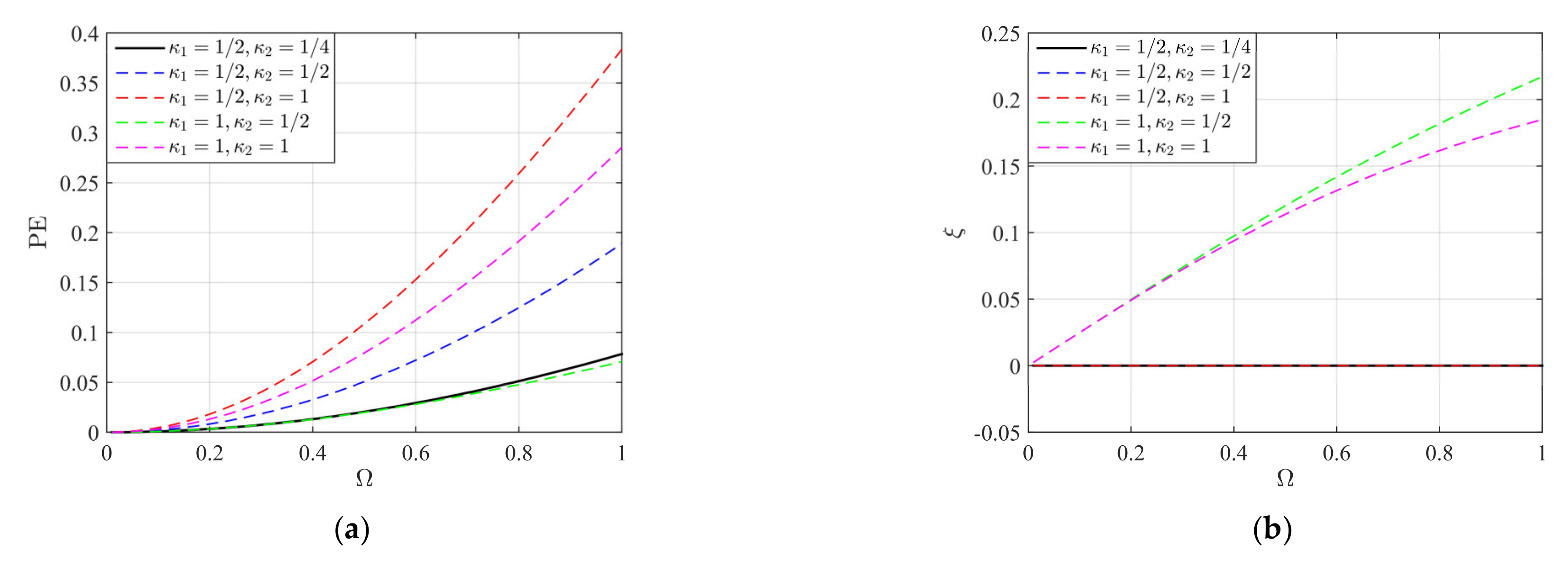
It was found that GCR algorithms with ${\kappa }_1$ and ${\kappa }_2$ possess numerical properties identical to the classical Newmark algorithms with γ and β. The mapping relation is $\left[{\kappa }_1, {\kappa }_2\left]=\right[\gamma , \beta \right]$. The CR algorithm is a special type of GCR algorithm, with ${\kappa }_1=1/2,{\kappa }_2=1/4$; its counterpart includes Newmark algorithms with $\gamma =1/2,\beta =1/4$, which is the well-known constant average acceleration (CAA) algorithm. The members of the subfamily of GCR algorithms with ${\kappa }_1=1/2$ have no numerical damping and are second-order accurate. GCR algorithms with $2{\kappa }_2\ge {\kappa }_1\ge 1/2$ are unconditionally stable for linear elastic systems. GCR algorithms with ${\kappa }_1>1/2, {\kappa }_2\ge {\left({\kappa }_1+1/2\right)}^2/4$ have numerical damping. The period elongation (PE) and equivalent damping ratios are two widely used indices of evaluating the accuracy of the integration algorithm [30]. The two accuracy indices of five GCR algorithms, i.e., $\left[{\kappa }_1, {\kappa }_2\left]=\right[1/2, 1/4\left], \right[1/2, 1/2\left],\right[1/2, 1\left],\right[1, 1/2\left], \right[1, 1\right]$, are depicted in Figure 1. The abscissa in Figure 1 is $\mathsf{\Omega }=\omega \Delta t$, where $\omega$ is the circular frequency. Figure 1 shows that for a certain ${\kappa }_1$, the PE increases with the increase in ${\kappa }_2$. GCR algorithms with $\left[{\kappa }_1, {\kappa }_2\left]=\right[1, 1/2\right]$ have PE close to that of $\left[1/2, 1/4\right]$(CR algorithm) and are minimum. Regarding the equivalent damping ratio, GCR algorithms with ${\kappa }_1=1/2$ are zero, whereas GCR algorithms with ${\kappa }_1=1$ are positive. Overall, the original CR algorithm has excellent accuracy and can be used as a reference for other GCR algorithms.

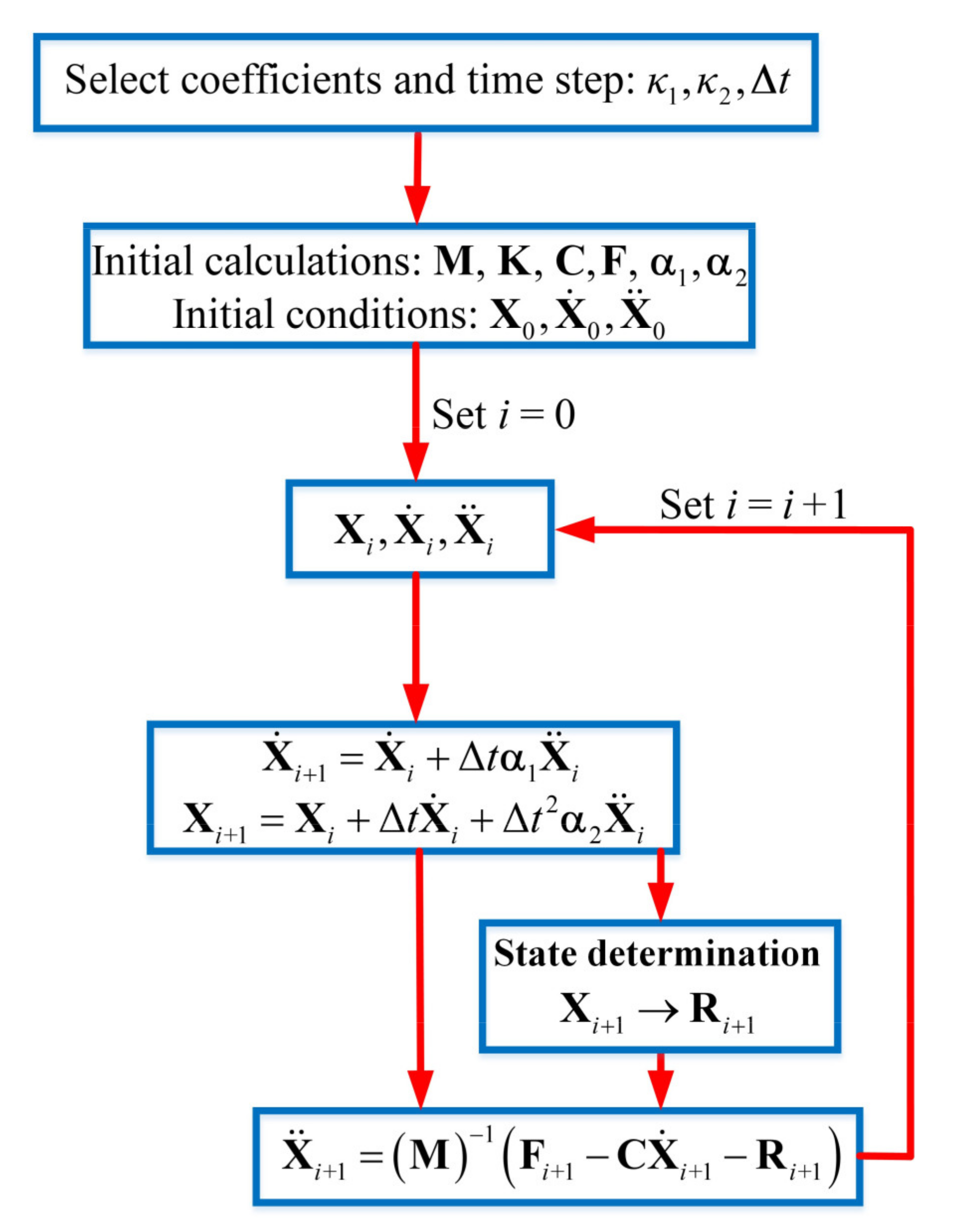
Figure 2 provides a general flowchart for solving the EOM for MDOF systems using GCR algorithms. The first step is to select appropriate integration coefficients ${\kappa }_1$ and ${\kappa }_2$ and the time step $\Delta t$. Then, the structural model matrices M, K, and C, and the external force F are calculated. The model-based integration parameter matrices ${\mathit{\alpha }}_1$ and ${\mathit{\alpha }}_2$ are then obtained using Equation (5). Then, the initial conditions are calculated as follows:

$${\ddot{X}}_0={\left(M\right)}^{-1}\left(F_0-C{\dot{X}}_0-K{X}_0\right)$$

(6)

where ${\dot{X}}_0$, $X_0$, and ${\ddot{X}}_0$ are the initial velocity, displacement, and acceleration, respectively.

Then, the difference equations of the GCR algorithms, i.e., Equation (3), are adopted to predict the velocity ${\dot{X}}_{i+1}$ and displacement $X_{i+1}$ at the next time step. The displacement $X_{i+1}$ can be used to determine the restoring force $R_{i+1}$, which is called state determination. If the structural system is linear elastic, the restoring force $R_{i+1}$ can be directly calculated as $K{X}_{i+1}$; otherwise, it can be obtained using the FE method, e.g., the FE modeling in Section 3. The final step is to calculate the acceleration by rewriting the EOM, i.e., Equation (1):

$${\ddot{X}}_{i+1}={\left(M\right)}^{-1}\left(F_{i+1}-C{\dot{X}}_{i+1}-R_{i+1}\right)$$

(7)

3. Finite Element Modeling of Frame Structure

In this study, stiffness-based beam-column elements with fiber sections along with P-Δ effects are adopted to simulate the frame structure. The stiffness-based beam-column elements are used to acquire the first-order restoring force, and the P-Δ effects are considered to obtain the second-order restoring force. The following content summarizes the basic principles and procedures.

3.1. Stiffness-Based Beam-Column Element with Fiber Sections

3.1.1. Initialization

The model-based integration parameter matrices, i.e., ${\mathit{\alpha }}_1$ and ${\mathit{\alpha }}_2$, should be predetermined before using model-based integration algorithms. As shown in Equation (5), model-based integration parameter matrices are functions of model matrices of structure, i.e., $M$, $C$, and $K$, and two controlling coefficients ${\kappa }_1$ and ${\kappa }_2$. Therefore, the first step is to find an appropriate combination of ${\kappa }_1$ and ${\kappa }_2$ based on the numerical properties of the GCR algorithms. Then, the model matrices of the structures should be determined. Among the three model matrices of structure, the Rayleigh damping assumption is widely adopted for establishing the damping matrix $C$:

$$C=a_{m}M+a_{k}K=\frac{2\xi {\omega }_i{\omega }_j}{{\omega }_i+{\omega }_j}M+\frac{2\xi }{{\omega }_i+{\omega }_j}K$$

(8)

where $a_m$ and $a_k$ are the combination coefficients of $M$ and $K$, respectively; $\xi$ is the damping ratio of structure; ${\omega }_i$ and ${\omega }_j$ are the ith and jth circular frequencies, respectively, which can be obtained by conducting modal analysis of the structure. Therefore, determination of the three model matrices is reduced to two matrices: $M$ and $K$.

The formulation of the mass matrix can be classified into two types: lumped mass and consistent mass. The detailed construction process can be found in [31].

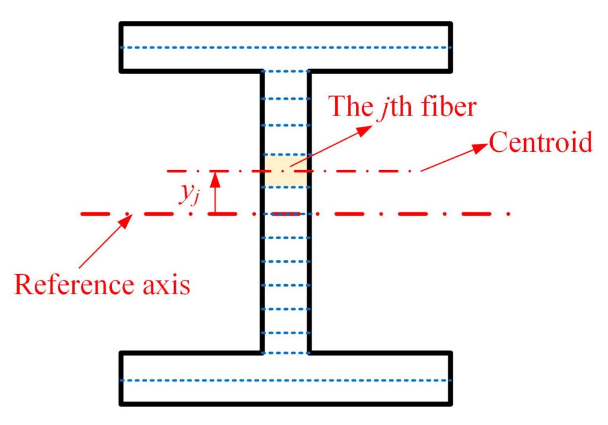
As a stiffness-based beam-column element with fiber sections is used, the initial stiffness matrix $K$ of the structure should be sequentially established from different levels. There are four levels from bottom to top: fiber, section, element, and structure. Regarding the section with fibers, the stiffness matrix ${\mathit{k}}_s\left(x\right)$ is:

$${\mathit{k}}_s\left(x\right)=\left[\begin{array}{cc}{{\displaystyle \sum }}_{j=1}^{N_f}{E}_j{A}_j& -{{\displaystyle \sum }}_{j=1}^{N_f}{E}_j{A}_j{y}_j\\ -{{\displaystyle \sum }}_{j=1}^{N_f}{E}_j{A}_j{y}_j& {{\displaystyle \sum }}_{j=1}^{N_f}{E}_j{A}_j{y}_j{}^2\end{array}\right]$$

(9)

where $E_j$, $A_j$, and $y_j$ are the elastic modulus, area, and centroid coordinate of the jth fiber, as shown in Figure 3; $N_f$ represents the total number of fibers for a section.

Then, the element stiffness matrix in the local coordinate system can be calculated as:

$${\overline{\mathit{k}}}_e={{\displaystyle \int }}_0^{L_e}{B}_d{\left(x\right)}^T{\mathit{k}}_s\left(x\right)B_d\left(x\right)dx$$

(10)

where $L_e$ is the element length; $B_d\left(x\right)$ is the differential of the displacement interpolation function with the expression of:

$$B_d\left(x\right)=\left[\begin{array}{cccccc}-\frac{1}{L_e}& 0& 0& \frac{1}{L_e}& 0& 0\\ 0& \frac{12x}{L_e{}^3}-\frac{6}{L_e{}^2}& \frac{6x}{L_e{}^2}-\frac{4}{L_e}& 0& \frac{6}{L_e{}^2}-\frac{12x}{L_e{}^3}& \frac{6x}{L_e{}^2}-\frac{2}{L_e}\end{array}\right]$$

(11)

It is impractical to integrate Equation (10) directly, so the Gauss–Legendre integration method is typically used to indirectly solve Equation (10). In this study, the Gauss–Legendre integration method with five integration points is used; then, Equation (10) can be rewritten as:

$${\overline{\mathit{k}}}_e={{\displaystyle \sum }}_{\mathit{k}=1}^5{B}_d{\left(x_k\right)}^T{k}_s\left(x_k\right)B_d\left(x_k\right){\omega }_k{L}_e$$

(12)

where $x_k$ and ${\omega }_k$ are the coordinate and weight at the kth integration point. The coordinates and weights of five integration points are listed in

Table 1. Coordinates and weights of five integration points of the Gauss–Legendre integration method.

k	1	2	3	4	5
$x_k$	0.046910 $L_e$	0.230765 $L_e$	0.500000 $L_e$	0.769234 $L_e$	0.953090 $L_e$
${\omega }_k$	0.118463	0.239314	0.284444	0.239314	0.118463

.

As the initial stiffness is elastic, direct use of the element stiffness matrix of the elastic beam-column element without fiber sections is also applicable and simpler (Equation (13)). The fiber section is adopted to formulate the element stiffness in order to make it consistent with the state determination in Section 3.1.2. It should be noted that the element stiffness matrix shown in Equation (13) is a symmetric matrix:

$${\overline{\mathit{k}}}_e=\left[\begin{array}{cccccc}EA/L_e& 0& 0& -EA/L_e& 0& 0\\ 0& 12EI/L_e{}^3& 6EI/L_e{}^2& 0& -12EI/L_e{}^3& 6EI/L_e{}^2\\ 0& 6EI/L_e{}^2& 4EI/L_e& 0& -6EI/L_e{}^2& 2EI/L_e\\ -EA/L_e& 0& 0& EA/L_e& 0& 0\\ 0& -12EI/L_e{}^3& -6EI/L_e{}^2& 0& 12EI/L_e{}^3& -6EI/L_e{}^2\\ 0& 6EI/L_e{}^2& 2EI/L_e& 0& -6EI/L_e{}^2& 4EI/L_e\end{array}\right]$$

(13)

where $E$ is the elastic modulus of the material; $A$ and $I$ are the area and inertia moment of the cross-section, respectively. It should be noted that only flexural deformation (without shear deformation) is considered in Equation (13).

Then, the element stiffness matrix ${\mathit{k}}_e$ in the global coordinate system can be transformed from the element stiffness matrix ${\overline{\mathit{k}}}_e$ in the local coordinate system:

$${\mathit{k}}_e={\mathit{T}}_e^T{\overline{\mathit{k}}}_e{\mathit{T}}_e$$

(14)

where ${\mathit{T}}_e$ is the coordinate transformation matrix. After calculating ${\mathit{k}}_e$ for all elements, the initial stiffness $K$ of the structure can finally be assembled by mapping the degrees of freedom (DOFs).

3.1.2. State Determination

State determination for using the stiffness-based beam-column element with fiber sections includes the following steps:

1.

Structure level: Predict the displacement $X_{i+1}$ at the (i + 1) time step using the GCR algorithms and obtain the incremental displacement $\Delta X_{i+1}=X_{i+1}-X_i$.

2.

Element level: Calculate the incremental element displacement $\Delta d_{e,i+1}$ in the global coordinate system by mapping the DOFs and transform it into the incremental element displacement $\Delta {\overline{d}}_{e,i+1}={\mathit{T}}_e\Delta d_{e,i+1}$ in the local coordinate system.

3.

Section level: The incremental section deformation $\Delta {\mathsf{\nu }}_{S,i}\left(x_k\right)$ at the integration points can be obtained as $\Delta {\mathsf{\nu }}_{S,i+1}\left(x_k\right)=B_d\left(x_k\right)\Delta {\overline{d}}_{e,i+1}={\left[\Delta \epsilon \left(x_k\right),\Delta \varphi \left(x_k\right)\right]}^T$, where $\Delta \epsilon \left(x_k\right)$ and $\Delta \varphi \left(x_k\right)$ are the incremental axial strain and curvature, respectively.

4.

Fiber level: The incremental strain of the jth fiber is $\Delta {\epsilon }_{j,i+1}=-\Delta \epsilon \left(x_k\right)+\Delta \varphi \left(x_k\right)y_j$. Then, the linear or nonlinear constitutive relationships of the material can be applied to obtain the stress ${\sigma }_{j,i+1}$ of the jth fiber.

5.

Section level: The section internal force $S_{i+1}\left(x_k\right)$ at the integration points can be assembled as $S_{i+1}\left(x_k\right)={\left[N_{i+1}\left(x_k\right),M_{i+1}\left(x_k\right)\right]}^T={\left[{{\displaystyle \sum }}_{j=1}^{N_f}{\sigma }_{j,i+1}{A}_j,{{\displaystyle \sum }}_{j=1}^{N_f}{\sigma }_{j,i+1}{A}_j{y}_j\right]}^T$.

6.

Element level: The element force ${\overline{f}}_{e,i+1}$ in the local coordinate system can be integrated by the section forces at the integration points as ${\overline{f}}_{e,i+1}={{\displaystyle \sum }}_{k=1}^5{B}_d{\left(x_k\right)}^T{S}_{i+1}\left(x_k\right){\omega }_k{L}_e$. Then, the element force $f_{e,i+1}={\mathit{T}}_e^T{\overline{f}}_{e,i+1}$ in the global coordinate system can be obtained.

7.

Structure level: The element forces of all elements can be assembled as the first-order restoring force $R_{i+1}$.

3.2. P-Δ Effects

In this study, the P-Δ effects are taken into account with the lean-on column, which is subjected to the gravity of each floor. The lean-on column is simulated by several bar elements and connected to the moment-resisting frame by a rigid diaphragm at each floor. The discretization of the cross-section, i.e., fiber section, is not used to simulate the bar elements of the lean-on column, which is assumed to behave elastically. The second-order restoring force is the product of the structural geometric stiffness $K_g$ and the structural displacement $X_{i+1}$. The structural geometric stiffness $K_g$ is the assembly of the geometric stiffness ${\mathit{k}}_g$ of the bar elements, which is expressed as:

$${\mathit{k}}_g=\frac{P}{L_e}\left[\begin{array}{cccc}1& 0& -1& 0\\ 0& 1& 0& -1\\ -1& 0& 1& 0\\ 0& -1& 0& 1\end{array}\right]$$

(15)

where $P$ is the gravity subjected to the lean-on column. It should be noted that the geometric stiffness is a symmetric matrix.

3.3. Time History Analysis of a Four-Story Frame Subjected to Earthquake

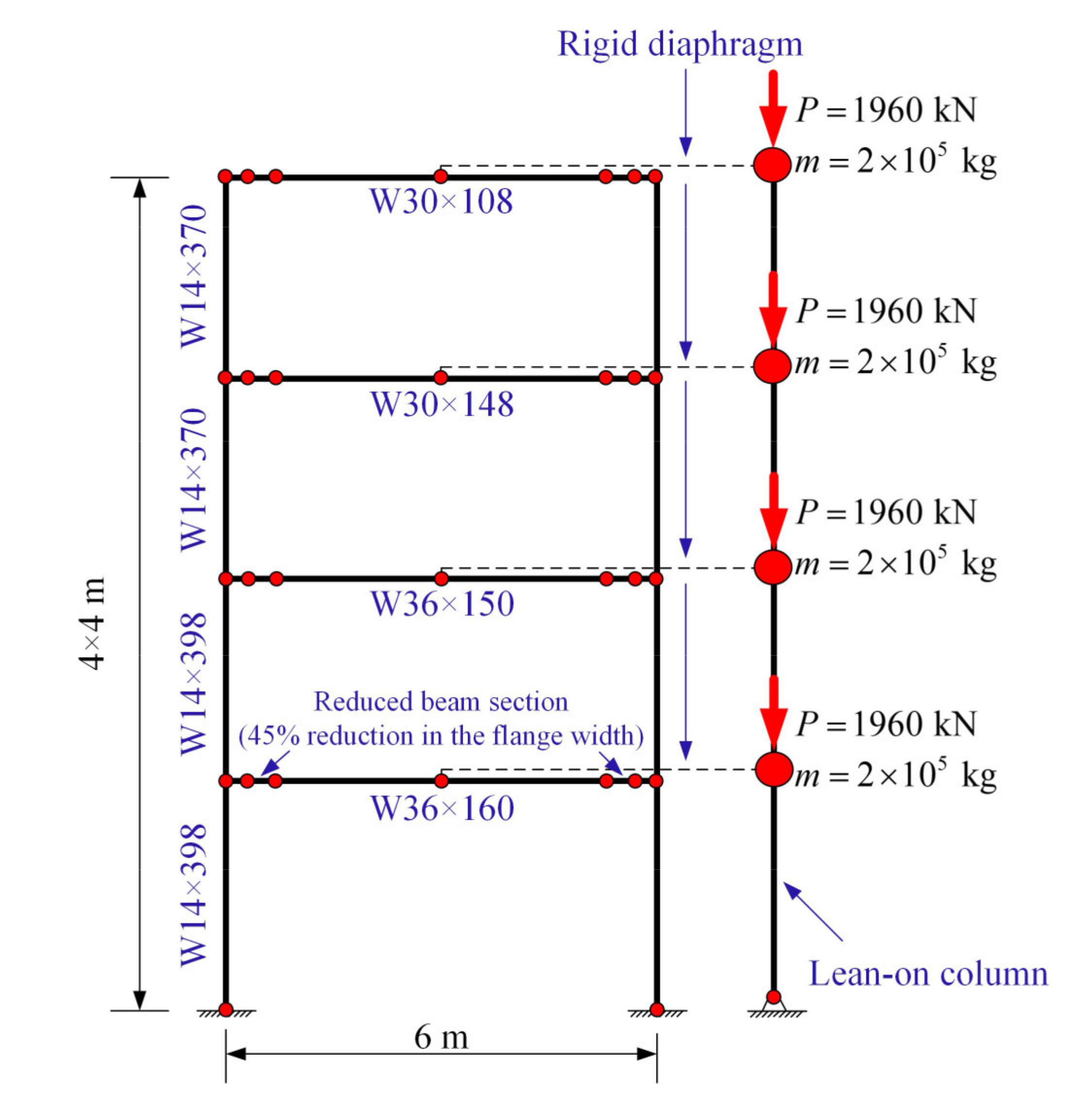
The primary structure is a four-story steel frame, as shown in Figure 4. The stiffness-based beam-column elements with fiber sections are used to simulate the beams and columns of the moment resisting frame, which is completely symmetric, and the bar elements are adopted to model the lean-on column. There are 24 fibers for each section of the beam-column elements. The elastic modulus and yield strength of the steel are 200 GPa and 345 MPa, respectively. The elastic–perfectly plastic constitutive relationship is adopted for steel. A consistent mass is used to build the mass matrix. The formulation of the initial stiffness matrix follows the procedure in Section 3.1. Shear deformation is not considered in the finite element model. According to the modal analysis, the first and second natural periods of the frame are 1.02 and 0.32 s, respectively. The Rayleigh damping assumption with a 2% damping ratio for the first and second order modes is applied to generate the damping matrix.

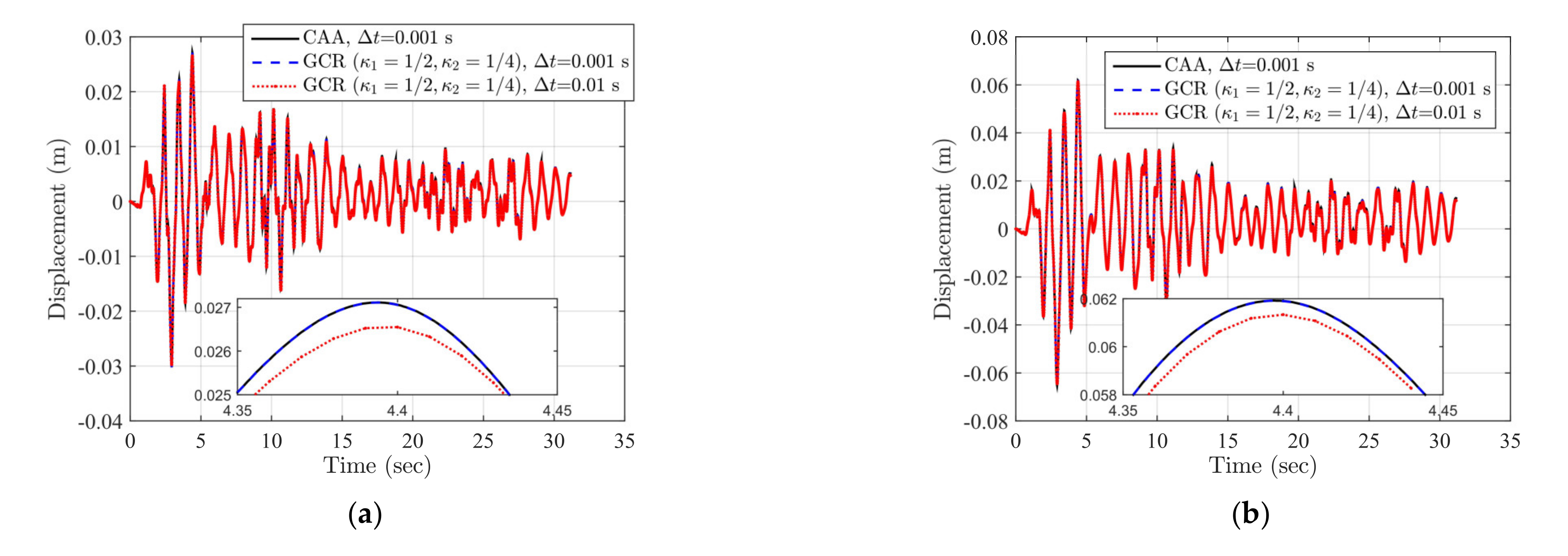
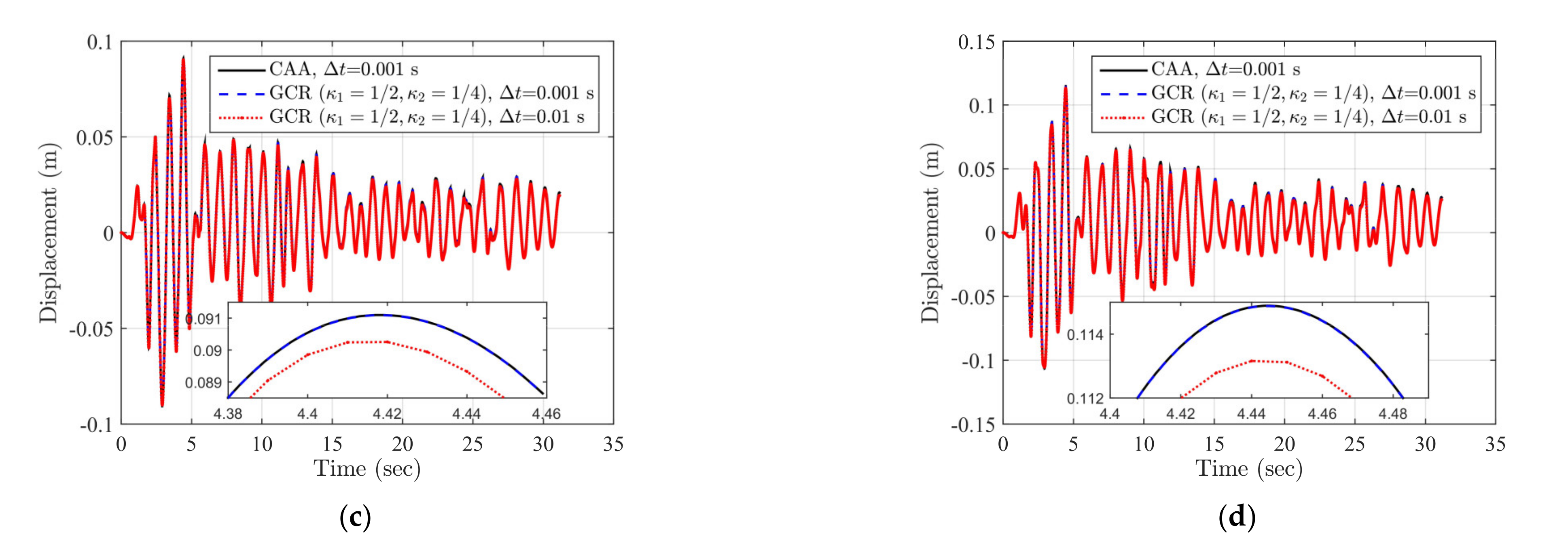
The structure is subjected to the unscaled 1940 El Centro NS ground motion. GCR algorithms with ${\kappa }_1=1/2,{\kappa }_2=1/4$ and two time steps of 0.01 and 0.001 s are used to conduct the time history analysis. The Newmark CAA algorithm with a time step of 0.001 s is taken for comparison. It should be noted that the GCR algorithms are explicit, whereas the CAA is implicit, so the computing efficiency of the GCR algorithms far exceeds that of the CAA algorithm with the same time step. If a larger time step is adopted, the efficiency of the GCR algorithm can be further improved. Figure 5 compares the lateral displacements of different stories using variant algorithm schemes.

Figure 5 shows that the numerical results of the GCR algorithms match well with those of the CAA algorithm. Furthermore, two error indices are adopted to measure the errors between the reference model (CAA) and computing models (GCR):

$$\mathrm{NEE}=\left|\frac{{{\displaystyle \sum }}_{i=1}^N{x}_{RM,i}^2-{{\displaystyle \sum }}_{i=1}^N{x}_{CM,i}^2}{{{\displaystyle \sum }}_{i=1}^N{x}_{CM,i}^2}\right|$$

(16)

$$\mathrm{NRMSE}=\frac{\sqrt{{{\displaystyle \sum }}_{i=1}^N\frac{{\left(x_{RM,i}-x_{CM,i}\right)}^2}{N}}}{\max \left(x_{CM}\right)-\min \left(x_{CM}\right)}$$

(17)

where $x_{RM}$ and $x_{CM}$ are the structural responses of the reference model and computing model, respectively; $N$ is the sampling number. NEE and NRMSE are sensitive to the amplitude and frequency errors, respectively.

Table 2. Error indices of lateral displacements using different integration algorithms (unit: %).

Integration Algorithm Scheme	Story	NEE	NRMSE
GCR (${\kappa }_1=1/2,{\kappa }_2=1/4$), Δt = 0.001 s	1	1.09 × 10−2	2.75 × 10−3
	2	1.49 × 10−2	3.26 × 10−3
	3	1.66 × 10−2	3.73 × 10−3
	4	1.62 × 10−2	3.95 × 10−3
GCR (${\kappa }_1=1/2,{\kappa }_2=1/4$), Δt = 0.01 s	1	2.33	0.64
	2	3.06	0.65
	3	3.54	0.73
	4	3.61	0.82

provides the corresponding error indices for Figure 5. It can be concluded from Table 2 that the differences between the GCR algorithms and the CAA algorithm with the same time step of 0.001 s are extremely small; even for the GCR algorithm with a larger time step of 0.01 s, the maximum NEE and NRMSE are less than 4% and 1%, respectively, which are acceptable in engineering practice. This indicates that GCR algorithms are viable for solving nonlinear dynamic problems with superior computational efficiency and accuracy.

4. Analytical Models of Dampers

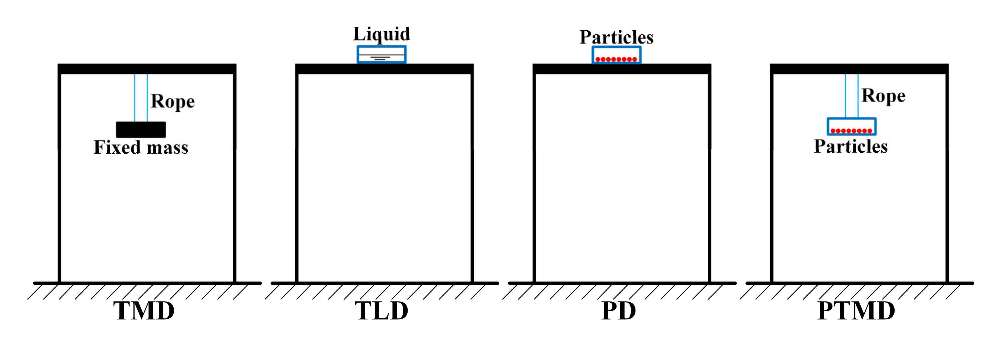
Four types of dampers, i.e., tuned mass dampers (TMDs), tuned liquid dampers (TLDs), particle dampers (PDs), and particle-tuned mass dampers (PTMDs), are selected to mitigate the seismic responses of the four-story steel frame. All four types of damper are installed on the top story and can be regarded as secondary structures to the primary structure, so they are ideal experimental substructures for SSTT. The four structure–damper systems are illustrated in Figure 6. The TMD can absorb the vibration energy at the tuned frequency and, therefore, reduce the structural response of the primary structure. The TLD is a tank containing liquid and can dissipate the vibration energy by liquid boundary layer friction, free surface contamination, and wave breaking. Similarly, the PD is a container equipped with particles that dissipate the energy by particle-to-particle and particle-to-container wall collision and friction. The PTMD is a combination of a TMD and PD, so it integrates the energy dissipation mechanisms of the two dampers.

4.1. Tuned Mass Damper (TMD)

The tuned mass damper (TMD) can be idealized as an SDOF system with mass, stiffness, and damping coefficients. To design a TMD, the mass ratio ${\gamma }_M$ is the first parameter that should be determined:

$${\gamma }_M=\frac{M_{TMD}}{M_s}$$

(18)

where $M_{TMD}$ and $M_s$ are the mass of the TMD and the primary structure, respectively. According to Section 3, the total mass of the primary structure is 8 × 10⁵ kg. Four TMDs with various auxiliary mass ratios, i.e., 1%, 2%, 3%, and 4%, are adopted. The corresponding mass of the TMD can easily be calculated using Equation (18).

According to the classical optimizing parameters for TMD proposed by Den Hartog [32], the optimized frequency ratio ${\gamma }_F$ and the damping ratio ${\xi }_{TMD}$ can be expressed as the function of ${\gamma }_M$:

$${\gamma }_F=\frac{f_{TMD}}{f_s}=\frac{1}{1+{\gamma }_M}$$

(19)

$${\xi }_{TMD}=\sqrt{\frac{3{\gamma }_M}{8\left(1+{\gamma }_M\right)}}$$

(20)

where $f_{TMD}$ and $f_s$ are the frequency of the TMD and the primary structure, respectively. The first-order frequency of the primary structure ($f_1=0.98 \mathrm{Hz}$) can be assigned to $f_s$. Other parameters of the TMD, such as stiffness $K_{TMD}=M_{TMD}{\left(2\pi f_{TMD}\right)}^2$ and damping coefficient $C_{TMD}=2M_{TMD}{\xi }_{TMD}\left(2\pi f_{TMD}\right)$, can be determined and are listed in

Table 3. Parameters of dampers with different mass ratios (mass unit: kg; stiffness unit: N/m; damping coefficient unit: N.s/m).

Auxiliary Mass Ratio	TMD	TLD	PD	PTMD
1%	MTMD = 8 × 103 KTMD = 2.95 × 105 CTMD = 5.92 × 103	MTLD = 8 × 103 KTLD = 2.05 × 105$\kappa$ CTLD = 8.11 × 104 ${\xi }_{TLD}\sqrt{\kappa }$	MPD = 8 × 103 KPD = 1.26 × 108 CPD = 4.02 × 106	MTMD = 1.6 × 103, MPD = 6.4 × 103 KTMD = 5.91 × 104, KPD = 1.01 × 108 CTMD = 1.18 × 103, CPD = 3.22 × 105
2%	MTMD = 1.6 × 104 KTMD = 5.79 × 105 CTMD = 1.65 × 104	MTLD = 1.6 × 104 KTLD = 4.11 × 105$\kappa$ CTLD = 1.62 × 105 ${\xi }_{TLD}\sqrt{\kappa }$	MPD = 1.6 × 104 KPD = 2.53 × 108 CPD = 8.04 × 106	MTMD = 3.2 × 103, MPD = 1.28 × 104 KTMD = 1.16 × 105, KPD = 2.02 × 108 CTMD = 3.30 × 103, CPD = 6.43 × 105
3%	MTMD = 2.4 × 104 KTMD = 8.52 × 105 CTMD = 2.99 × 104	MTLD = 2.4 × 104 KTLD = 6.16 × 105$\kappa$ CTLD = 2.43 × 105 ${\xi }_{TLD}\sqrt{\kappa }$	MPD = 2.4 × 104 KPD = 3.79 × 108 CPD = 1.21 × 106	MTMD = 4.8 × 103, MPD = 1.92 × 104 KTMD = 1.70 × 105, KPD = 3.03 × 108 CTMD = 5.98 × 103, CPD = 9.65 × 105
4%	MTMD = 3.2 × 104 KTMD = 1.11 × 106 CTMD = 4.54 × 104	MTLD = 3.2 × 104 KTLD = 8.21 × 105$\kappa$ CTLD = 3.24 × 105 ${\xi }_{TLD}\sqrt{\kappa }$	MPD = 3.2 × 104 KPD = 5.05 × 108 CPD = 1.61 × 106	MTMD = 6.4 × 103, MPD = 2.56 × 103 KTMD = 2.23 × 105, KPD = 4.04 × 108 CTMD = 9.07 × 103, CPD = 1.29 × 106

.

4.2. Tuned Liquid Damper (TLD)

There are several existing analytical or numerical models for TLD. According to [33], the TLD model developed by Yu et al. [34] has good predictions in both weak and strong wave breaking and in a broad range of frequency ratios. Therefore, Yu et al.’s model is adopted in this study.

Yu et al.’s model is an equivalent nonlinear-stiffness–damping (NSD) model of the TLD. The structural parameters of the TLD model are summarized as follows.

1.

Mass: Assume the mass $M_{TLD}$ of TLD equals the mass of liquid; that is, the mass of the container is neglected. Water is typically used as the liquid, so $M_{TLD}$ can be calculated as $M_{TLD}=M_w={\rho }_{w}BLh$, where ${\rho }_w$ is the density of water; $B$ and $L$ are the width and length (the excitation direction) of the rectangular tank, respectively; $h$ is the water depth.

2.

Stiffness: The initial linear stiffness of TLD is $K_w=M_{TLD}{\left(2\pi f_w\right)}^2$, where $f_w$ is the linear fundamental natural frequency for water and expressed as:

$$f_w=\frac{\sqrt{\frac{\pi g}{L}\tanh \left(\frac{\pi h}{L}\right)}}{2\pi }$$

(21)

where $g$ is the gravitational constant. According to Yu et al. [34], the nonlinear stiffness $K_{TLD}$ of TLD can be determined by the stiffness hardening ratio of $\kappa$ and $K_w$:

$$\kappa =\frac{K_{TLD}}{K_w}={\left(\frac{f_{TLD}}{f_w}\right)}^2=\left\{\begin{array}{c}1.075{\mathsf{\Lambda }}^{0.007},\mathrm{for} \mathsf{\Lambda }\le 0.03 \mathrm{weak} \mathrm{wave} \mathrm{breaking}\\ 2.52{\mathsf{\Lambda }}^{0.25}, \mathrm{for} \mathsf{\Lambda }>0.03 \mathrm{strong} \mathrm{wave} \mathrm{breaking}\end{array}\right.$$

(22)

$$K_{TLD}=M_{TLD}\kappa \frac{\pi g}{L}\tanh \left(\frac{\pi h}{L}\right)$$

(23)

where $\mathsf{\Lambda }=A/L$ is the non-dimensional displacement amplitude, and $A$ is the displacement amplitude of excitation.

3.

Damping: The damping coefficient of the TLD can be obtained as $C_{TLD}=2M_{TLD}{\xi }_{TLD}\left(2\pi f_{TLD}\right)$, where the damping ratio ${\xi }_{TLD}$ is also a function of $\mathsf{\Lambda }$:

$${\xi }_{TLD}=0.5{\mathsf{\Lambda }}^{0.35}$$

(24)

$$C_{TLD}=2M_{TLD}{\xi }_{TLD}\sqrt{\kappa \frac{\pi g}{L}\tan \mathrm{h}\left(\frac{\pi h}{L}\right)}$$

(25)

To design a TLD, the first parameter is also the mass ratio ${\gamma }_M$, which is the ratio of $M_{TLD}$ to $M_s$. In the same manner as for the TMDs, four TLDs with various auxiliary mass ratios, i.e., 1%, 2%, 3%, and 4%, are adopted. The tank length $L$ is assigned as a constant: 1 m. To achieve the maximum effectiveness of the TLD, the nonlinear natural frequency $f_{TLD}$ of the TLD should be equal to the natural frequency $f_s$ of the primary structure. Then, the water depth $h$ is determined as:

$$h=\frac{L}{\pi }{\tan \mathrm{h}}^{-1}\left(\frac{4\pi L{f}_s^2}{g\kappa }\right)$$

(26)

Based on the numerical results presented in Section 3, the displacement amplitude $A$ of the fourth story is 0.1149 m; the non-dimensional displacement amplitude $\mathsf{\Lambda }$ and the corresponding stiffness hardening ratio $\kappa$ can be calculated. By substituting the values of $L$, $\kappa$, and $f_s$ into Equation (26), the water depth $h$ is determined to be 0.3821 m. Therefore, the mass for a certain TLD is a constant, whereas the stiffness and damping are displacement amplitude-related variables and should be updated during time-history analysis. The parameters of the four TLDs with different mass ratios are also listed in Table 3.

4.3. Particle Damper (PD)

The conventional computing model of the PD uses the discrete element method (DEM), which is very time consuming and complicated. Based on correlational studies by Papalou and Masri [35], Lu et al. [3] proposed a simplified analytical method for the PD. The simplified model has been verified to have computational efficiency and a satisfactory degree of accuracy in practical applications. Therefore, Lu et al.’s model is adopted in this study.

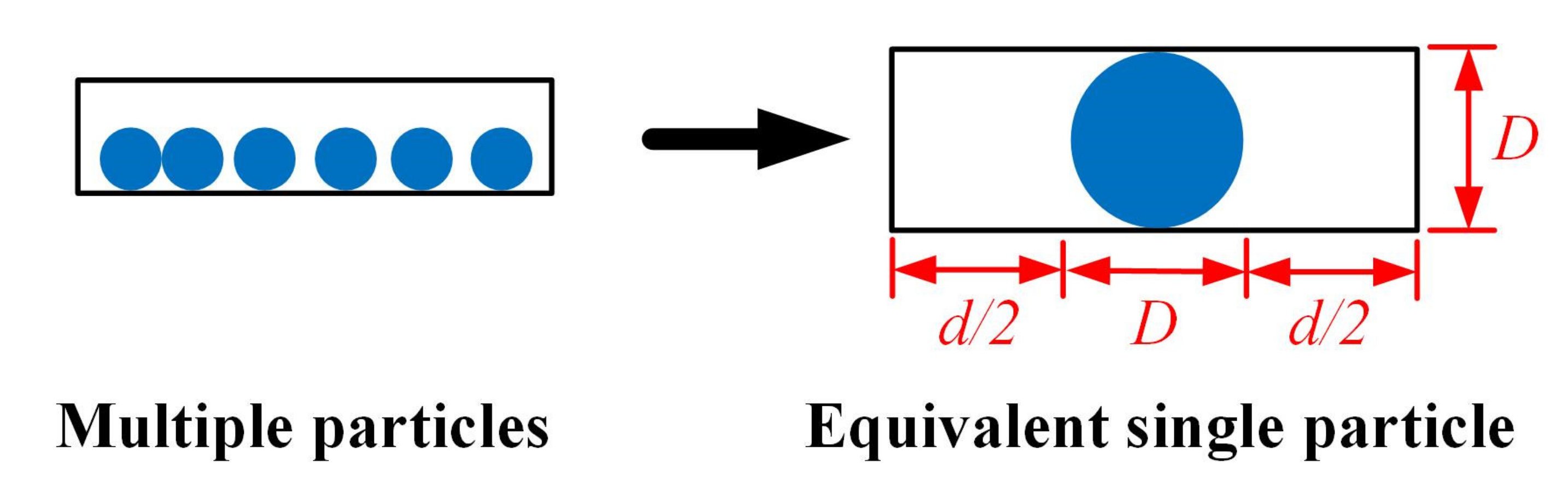
The essence of the model is to transform multiple particles into an equivalent single particle, as shown in Figure 7. The mass of the single particle equals the total mass of the multiple particles, assuming that the collisions between the particles can be neglected; then, the damping forces of the PD mainly originate from the collisions between the particles and the container wall.

In Figure 7, the clearance d of the single particle is a critical parameter governing the damping force and can be determined by the following equation:

$$\left(\frac{1}{{\rho }_{PD}}-1\right)\frac{M_{PD}}{\rho }=\frac{M_{PD}}{2\rho }+\frac{\pi }{4}{\left(\frac{6M_{PD}}{\pi \rho }\right)}^{\frac{2}{3}}d$$

(27)

where $M_{PD}$ is the mass of the PD; $\rho$ is the density of the particle material; ${\rho }_{PD}$ is the packing density of the multiple particles. Hales et al. [36] suggested that ${\rho }_{PD}$ should not exceed 0.74; a value of 0.6 is assigned to ${\rho }_{PD}$.

The mass $M_{PD}$ of PD is the product of the mass ratio ${\gamma }_M$ and the mass $M_s$ of the primary structure. Four mass ratios ranging from 1% to 4% are selected. The stiffness $K_{PD}$ of the equivalent single PD is determined as $K_{PD}=M_{PD}{\left(2\pi f_{PD}\right)}^2$. Masri and Ibrahim [37] recommended that $f_{PD}\ge 20f_1$, so the frequency of PD is set as $20f_1\approx 20 \mathrm{Hz}$. The damping coefficient $C_{PD}$ of the equivalent single PD can be written as $C_{PD}=2M_{PD}{\xi }_{PD}\left(2\pi f_{PD}\right)$, where the damping ratio ${\xi }_{PD}$ is related to the coefficient of restitution $e$ [38]. In this study, a steel particle with $e=0.5$ is adopted; thus, ${\xi }_{PD}$ is determined to be 0.2. The damping force of the single PD can be expressed as:

$$f_{PD}=C_{PD}H\left(x_{PD}^r,{\dot{x}}_{PD}^r\right)+K_{PD}G\left(x_{PD}^r\right)$$

(28)

where $x_{PD}^r$ and ${\dot{x}}_{PD}^r$ are the relative displacement and velocity of the PD with respect to the primary structure. $H\left(x_{PD}^r,{\dot{x}}_{PD}^r\right)$ and $G\left(x_{PD}^r\right)$ are two nonlinear functions with the expressions of:

$$H\left(x_{PD}^r,{\dot{x}}_{PD}^r\right)=\left\{\begin{array}{c}{\dot{x}}_{PD}^r,for x_{PD}^r\le -d/2 and x_{PD}^r\ge -d/2\\ 0,for-d/2<x_{PD}^r<d/2\end{array}\right.$$

(29)

$$G\left(x_{PD}^r\right)=\left\{\begin{array}{c}{x}_{PD}^r+d/2,\mathrm{for} x_{PD}^r\le -d/2\\ 0,\mathrm{for}-d/2<x_{PD}^r<d/2\\ x_{PD}^r-d/2,\mathrm{for} x_{PD}^r\ge d/2\end{array}\right.$$

(30)

4.4. Particle-Tuned Mass Damper (PTMD)

The particle-tuned mass damper (PTMD) is the combination of TMD and PD. The simplified analytical model proposed by Lu et al. [3] is also adopted. The PTMD can be idealized as a 2DOF system, which includes an SDOF TMD connected to the primary structure and an SDOF PD attached to the TMD. For the PTMD, the mass of the container cannot be neglected because it constitutes the TMD. Therefore, the total auxiliary mass of the PTMD is divided into two parts: PD and TMD. Lu et al. [3] investigated the influence of the ratio of the particle mass ($M_{PD}$) to the total auxiliary mass ($M_{PTMD}$) on the structural control effects of PTMD and found that the vibration attenuation of the PTMD can be improved to a certain extent by increasing the mass proportion of the PD. Therefore, an 80% mass ratio of $M_{PD}$ to $M_{PTMD}$ is used. Four PTMDs with varying auxiliary mass ratios from 1% to 4% are selected. The parameters of the TMD and PD are determined following the procedures presented in Section 4.1 and Section 4.3, respectively. The corresponding parameters of PTMDs can be found in Table 3.

5. Modeling of Substructure Shake Table Testing of Frame Structure–Damper System

5.1. Procedure of Substructure Shake Table Testing of Frame Structure–Damper System

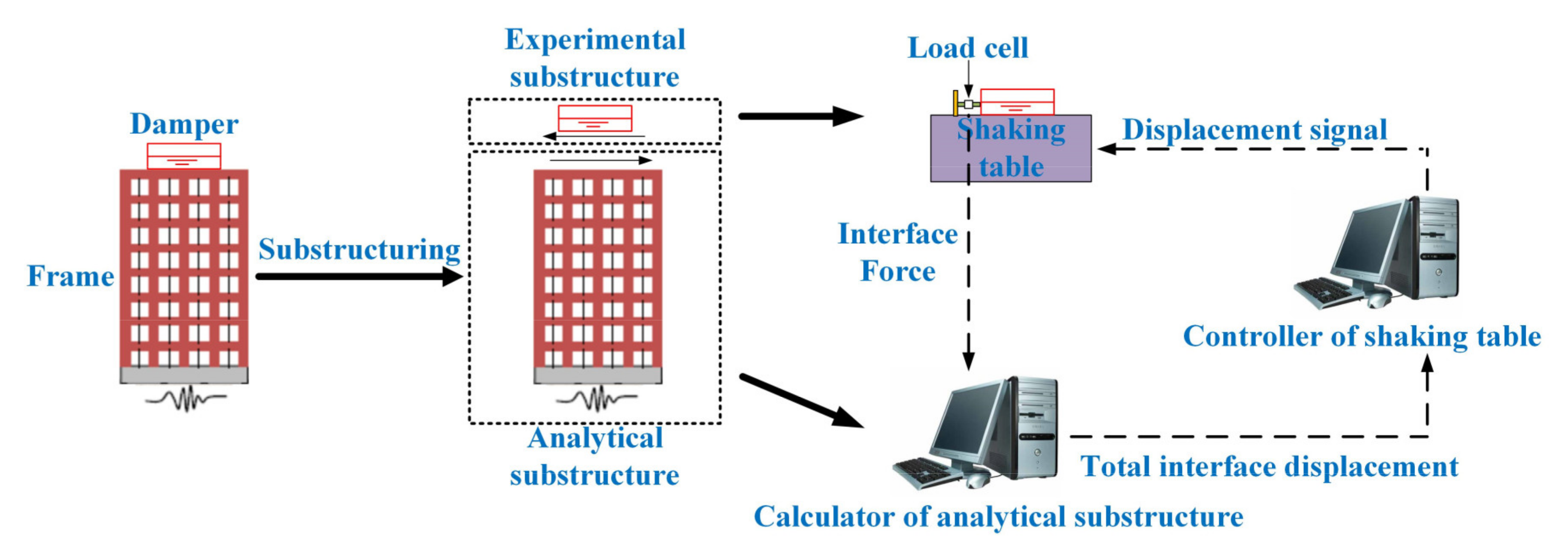
To carry out SSTT of the frame structure–damper system, the primary structure (frame) and the secondary structure (damper) are assigned as the analytical and experimental substructures, respectively. The analytical substructure is numerically simulated, and the damper is mounted on and excited by the shake table [15,16]. A schematic diagram of SSTT of the frame structure–damper system is illustrated in Figure 8.

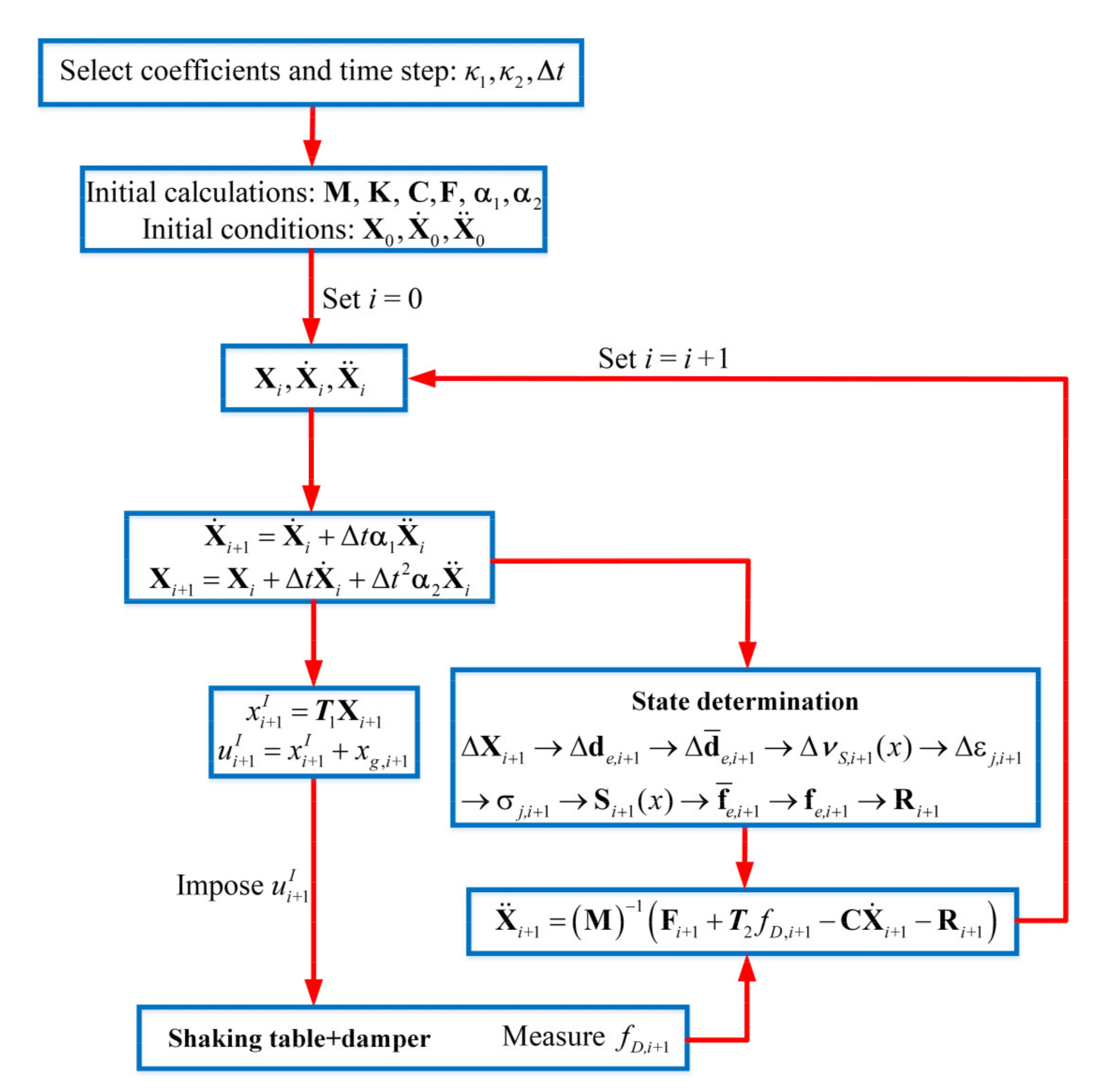
Figure 9 shows a flowchart of SSTT of the frame structure–damper system using GCR algorithms and the finite element method.

In Figure 8 and Figure 9, it should be noted that the excitation signal of the shake table is the total displacement at the interface instead of the relative displacement. Therefore, two additional calculation steps are required:

$$x_{i+1}^I={\mathit{T}}_1{X}_{i+1}$$

(31)

$$u_{i+1}^I=x_{i+1}^I+x_{g,i+1}$$

(32)

where $x_{i+1}^I$ and $u_{i+1}^I$ are the relative and total displacements at the interface, respectively; $x_{g,i+1}$ is the ground displacement; ${\mathit{T}}_1$ is the matrix transforming the DOFs of the structure to the interface DOF.

In addition, the EOM of the primary structure should be modified due to introduction of the damper force (interface force):

$$M{\ddot{X}}_{i+1}+C{\dot{X}}_{i+1}+R_{i+1}=F_{i+1}+{\mathit{T}}_2{f}_{D,i+1}$$

(33)

where $f_{D,i+1}$ is the damper force; ${\mathit{T}}_2$ is the matrix converting the interface DOF to the DOFs of the structure. This study aimed to conduct a series of virtual SSTTs, so the damper forces of the four types of dampers are numerically simulated instead of experimentally measured in a real SSTT. All numerical simulations were performed using MATLAB software and the Simulink toolbox.

5.2. Numerical Results and Discussions

It can be seen from Figure 8 and Figure 9 that the SSTT system is composed of four parts: the experimental substructure (damper), the analytical substructure (frame), the integration algorithm, and the shake table. Therefore, all four components influence the results of the SSTT system. The four-story frame in Section 3.3 is taken as the analytical substructure and remains unchanged. The four types of damper in Section 4 with different auxiliary mass ratios are taken as the experimental substructures. Therefore, the effects of the auxiliary mass ratio are investigated first. As discussed in Section 2, the integration parameters ${\kappa }_1$ and ${\kappa }_2$ greatly influence the numerical properties of the GCR algorithms. Thus, the effects of different sets of integration parameters are considered. Similarly, the time step is a critical factor determining the accuracy of the integration algorithm, and thus, is also studied. Finally, the time delay, which is a critical property of the shake table dynamics, is also taken into account.

5.2.1. Effects of the Auxiliary Mass Ratio

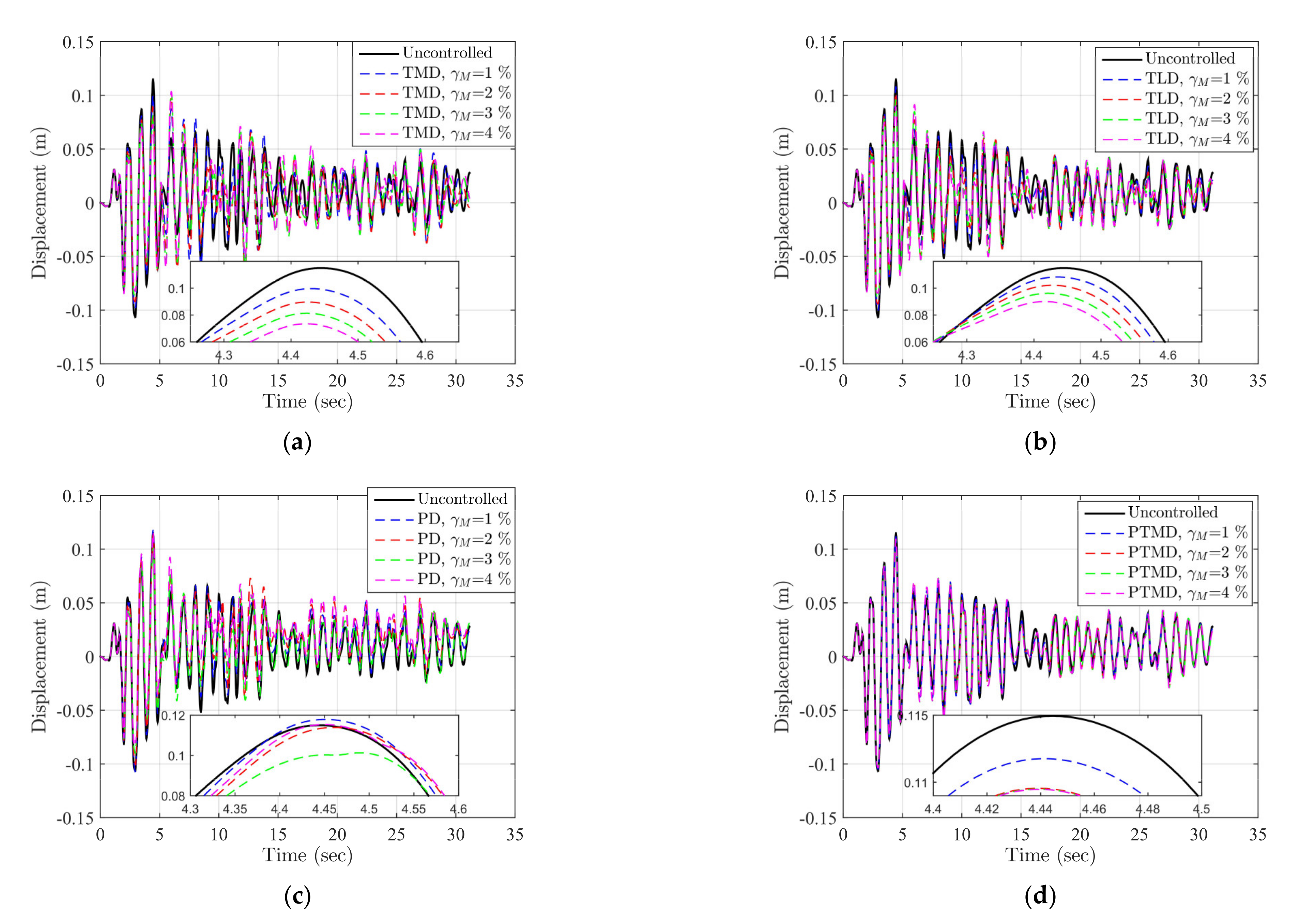
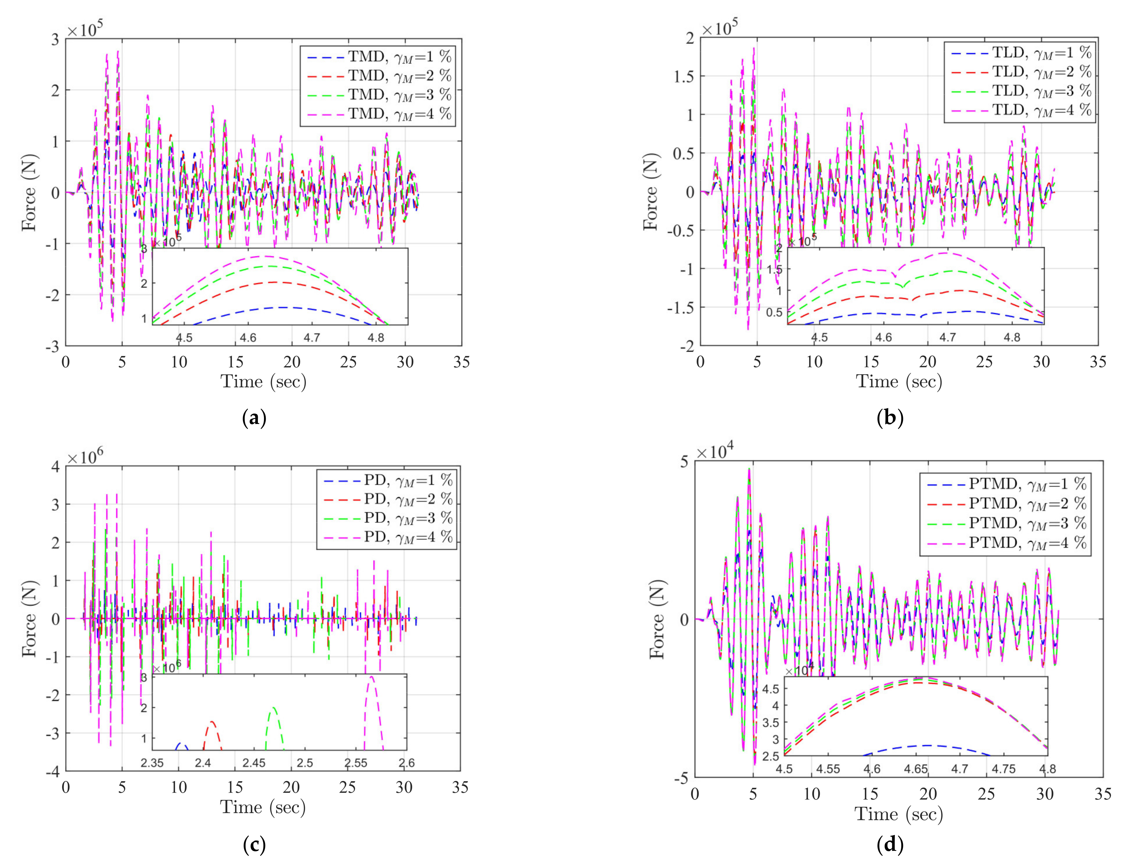
GCR algorithms with ${\kappa }_1=1/2,{\kappa }_2=1/4$ and a time step of 0.001 s are adopted to solve the virtual SSTT of the four-story steel frame (Section 3) with four types of damper (Section 4). Figure 10 shows the lateral displacements at the fourth story for the steel frame, in addition to four dampers with four auxiliary mass ratios. The seismic responses of the uncontrolled structure without dampers are used for comparison. The corresponding damper forces are provided in Figure 11. Two widely used reduction factors based on the maximum and root-mean-square (RMS) structural responses are used to quantify the reduction effects of dampers:

$$R_{\max }=1-\frac{\max \left|x_{controlled}\right|}{\max \left|x_{uncontrolled}\right|}$$

(34)

$$R_{\mathrm{RMS}}=1-\frac{\mathrm{RMS}\left(x_{controlled}\right)}{\mathrm{RMS}\left(x_{uncontrolled}\right)}$$

(35)

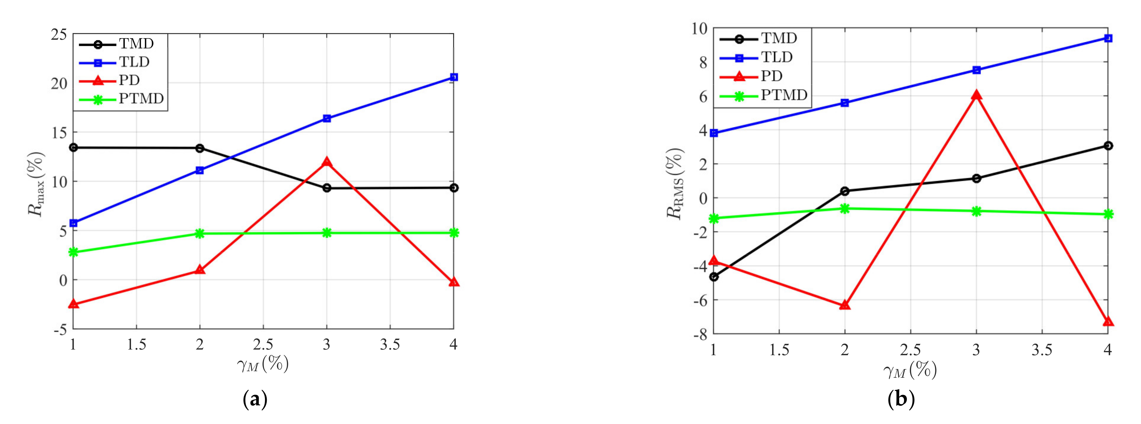
where $x_{controlled}$ and $x_{uncontrolled}$ are the structural responses of the controlled structure with dampers and the uncontrolled structure without dampers, respectively. The two reduction effects of the different dampers with varying mass ratios are compared in Figure 12.

Figure 10 and Figure 12 show that the TLD has the best performance in vibration control among the four dampers. Both the reduction factors of the TLD linearly increase with respect to the mass ratio. This result is consistent with the shake table results of structure–damper systems, such as [3,16]. Most TMDs possess positive vibration reduction effects, with the exception of $R_{\mathrm{RMS}}$ of the TMD, with a mass ratio of 1%. The $R_{\mathrm{RMS}}$ of the TMD increases with the increase in mass ratio. According to [6], the mass ratio of the TMD can only reach 0.1%–5% due to installation difficulties and economic costs. These mass ratios are much smaller than the optimal mass ratio, so the limited tuned mass cannot effectively reduce the structural vibrations. This explains the fair performance of the TMDs. A PD with a mass ratio of 3% has a satisfactory performance in terms of both $R_{\max }$ and $R_{\mathrm{RMS}}$, whereas it does not provide a positive control effect for other mass ratios. The mass ratio has negligible influence on the reduction effects of the PTMD. The $R_{\max }$ of the PTMDs is positive, whereas the $R_{\mathrm{RMS}}$ is negative. Figure 11 shows that the damper forces have a positive correlation with the mass ratios. In addition, the damper forces of the PDs have a magnitude of 10⁶ N, which is much larger than those of the counterpart TLDs. This indicates that a larger damper force cannot ensure better control performance. In sum, for the particular structure and ground motion in this study, these dampers are not always effective at controlling the seismic responses of the four-story steel frame. According to previous studies [3,6,7,8,9,10], the control performance of dampers is influenced by many factors, such as the dynamic characteristics of the primary structure, the frequency characteristics and intensities of the seismic inputs, and the damper parameters. Therefore, the conclusions drawn from Figure 10, Figure 11 and Figure 12 are specific and not generalizable.

5.2.2. Effects of the Integration Parameters of GCR Algorithms

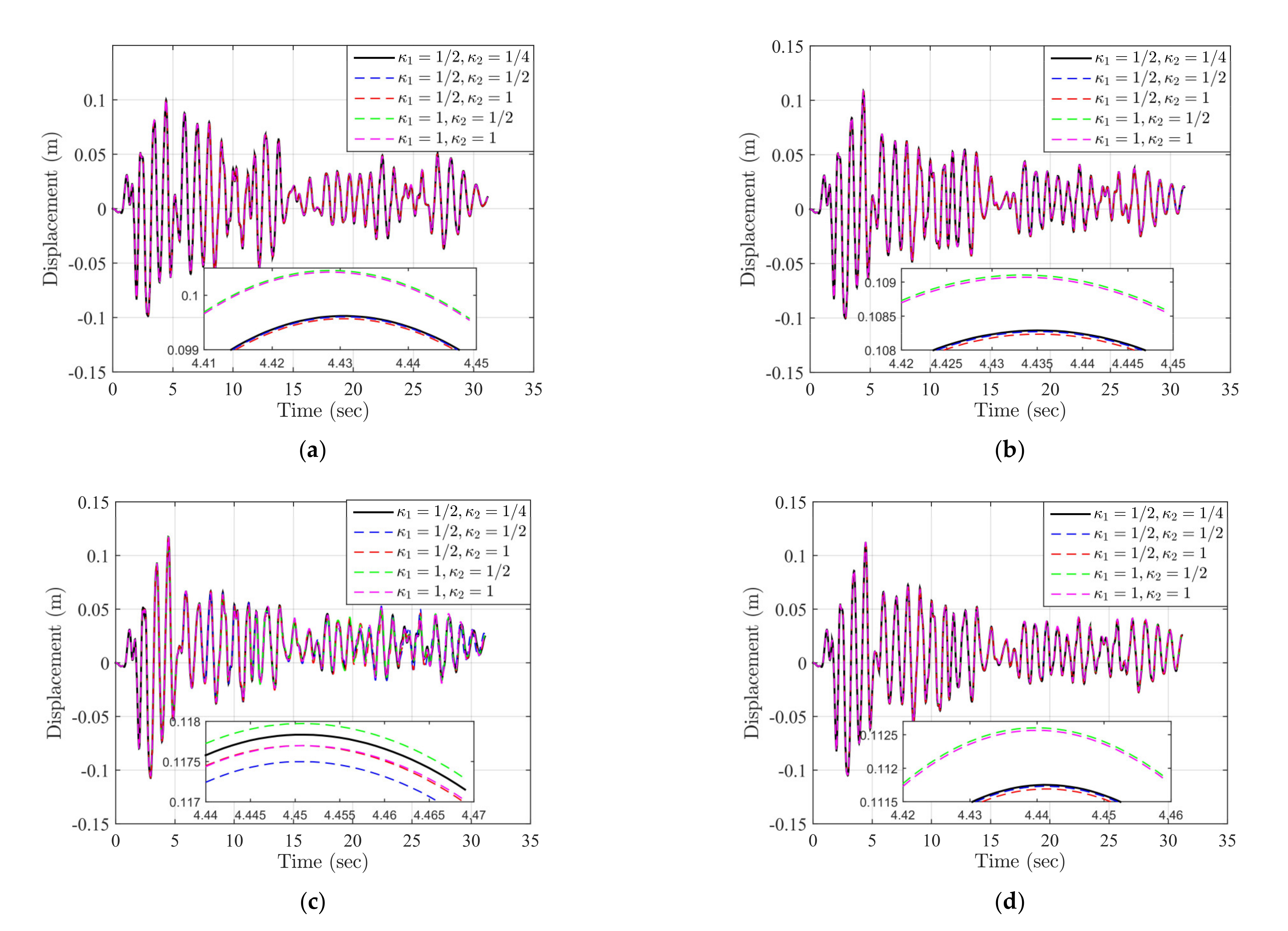
As mentioned in Section 2, the integration parameters, i.e.,${\kappa }_1$ and ${\kappa }_2$, of the GCR algorithms may greatly influence the numerical properties of the algorithms. Therefore, the influences of the two integration coefficients on SSTT are investigated. GCR algorithms with four sets of $\left[{\kappa }_1, {\kappa }_2\left]=\right[1/2, 1/2\left],\right[1/2, 1\left],\right[1, 1/2\left], \right[1, 1\right]$ are selected, whereas GCR algorithms with ${\kappa }_1=1/2,{\kappa }_2=1/4$ are used as the reference model. A time step of 0.001 s is adopted for the integration algorithms. The structural responses of the steel frame with four dampers with a mass ratio of 1% are considered. Figure 13 depicts the lateral displacement at the fourth story using GCR algorithms with different sets of integration coefficients.

Table 4. Error indices of top lateral displacements with different integration parameters (unit: %).

Integration Parameters	Damper	NEE	NRMSE
${\kappa }_1=1/2,{\kappa }_2=1/2$	TMD	2.68 × 10−2	6.80 × 10−3
	TLD	3.86 × 10−2	9.19 × 10−3
	PD	1.48	1.77
	PTMD	1.05 × 10−2	1.66 × 10−2
${\kappa }_1=1/2,{\kappa }_2=1$	TMD	7.98 × 10−2	2.03 × 10−2
	TLD	0.12	2.76 × 10−2
	PD	2.49	1.31
	PTMD	1.50 × 10−2	4.92 × 10−2
${\kappa }_1=1,{\kappa }_2=1/2$	TMD	0.76	0.35
	TLD	0.30	0.37
	PD	1.26	0.83
	PTMD	0.45	0.52
${\kappa }_1=1,{\kappa }_2=1$	TMD	0.80	0.35
	TLD	0.37	0.36
	PD	0.43	0.81
	PTMD	0.46	0.53

further provides the error indices of the structural responses.

Figure 13 and Table 4 show that the error indices of the PDs are generally larger than their counterpart TMDs, TLDs, and PTMDs, particularly when ${\kappa }_1=1/2,{\kappa }_2=1/2$ and ${\kappa }_1=1/2,{\kappa }_2=1$. In addition, the error indices of ${\kappa }_1=1$ normally exceed those of ${\kappa }_1=1/2$ because there exists numerical damping for GCR algorithms with ${\kappa }_1=1$, as shown in Figure 1. However, all the error indices are relatively small (the maximum NEE and NRMSE are less than 3%). This can be explained as follows: the fundamental frequency of the frame structure $f_1$ is 0.98 Hz, thus the corresponding $\mathsf{\Omega }=2\pi f_1\Delta t=0.006$. As the value of $\mathsf{\Omega }$ is small, the PE and equivalent damping ratio, as indicated in Figure 1, of the integration algorithm is very small. For instance, when ${\kappa }_1=1,{\kappa }_2=1$, the PE and equivalent damping ratios of the GCR algorithms are only 1.2 × 10⁻⁵ and 0.0015, respectively. The relatively low error of the integration algorithm leads to small errors in the SSTT results. Therefore, the influences of the integration parameters of the GCR algorithms on SSTT of the frame structure with dampers can be neglected. It should be noted, however, that if a larger time step and a stiffer structure with a larger frequency are adopted, the influences of the integration parameters may be significant.

5.2.3. Effects of the Time Step

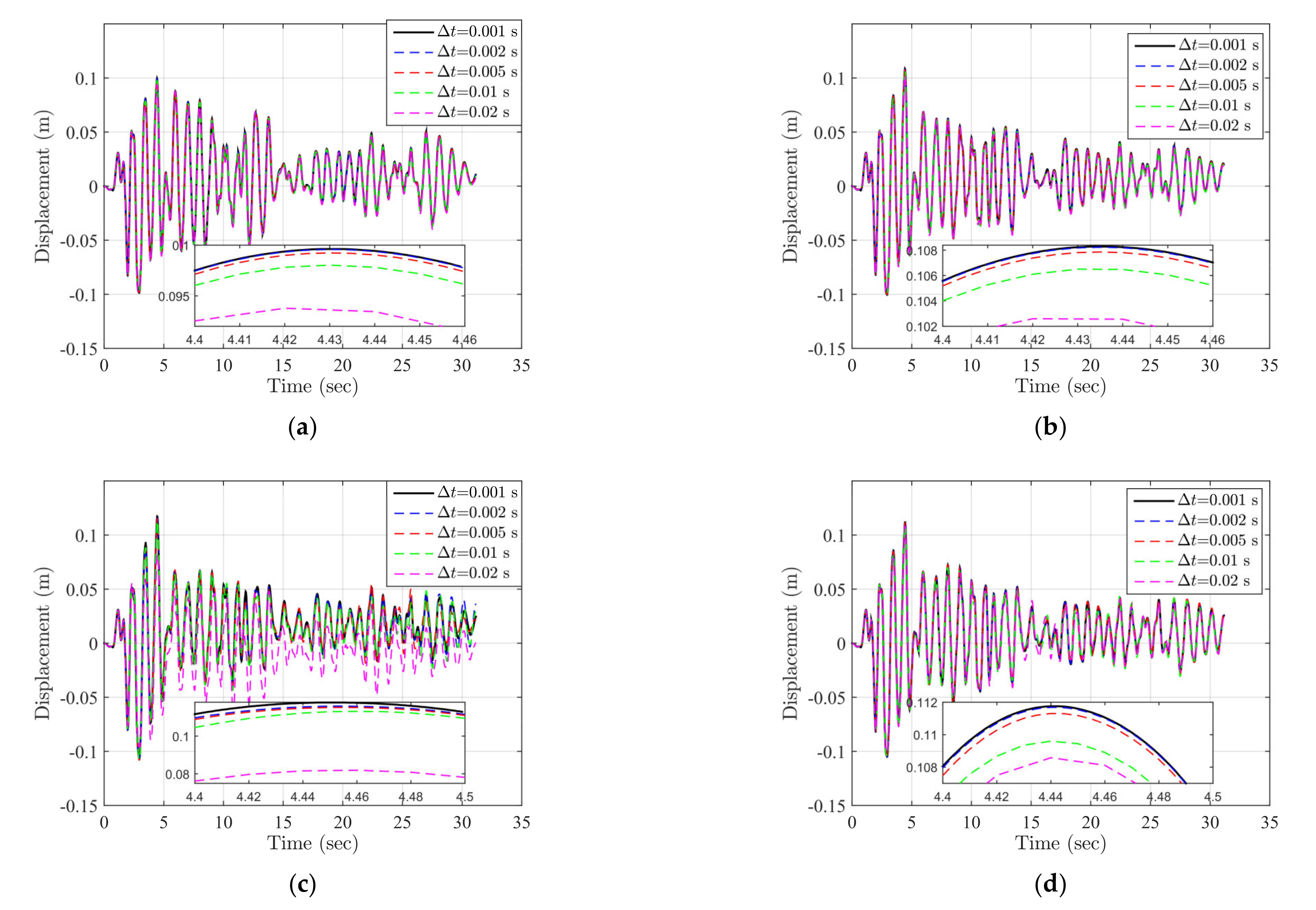
The time step is a crucial factor of the integration algorithms and SSTT. A larger time step means saving more computing time while reducing accuracy. It is well known that SSTT requires high computational efficiency for integration algorithms. If an integration algorithm maintains a relatively high accuracy for a larger time step, it is definitely a promising choice for the application of SSTT. Therefore, we studied the influence of the time steps on SSTT. GCR algorithms with ${\kappa }_1=1/2,{\kappa }_2=1/4$ and four time steps ($\Delta t=0.002 \mathrm{s}, 0.005 \mathrm{s}, 0.01\mathrm{s}, 0.02 \mathrm{s}$) are adopted. The results for GCR algorithms with ${\kappa }_1=1/2,{\kappa }_2=1/4$ and a time step of $\Delta t=0.001 \mathrm{s}$ are used for comparison. The lateral displacements at the top story and the steel frame attached to the four types of dampers with a mass ratio of 1% are provided in Figure 14. The corresponding error indices are tabulated in

Table 5. Error indices of top lateral displacements with different time steps (unit: %).

Time Step	Damper	NEE	NRMSE
$\Delta t=0.002 \mathrm{s}$	TMD	7.14 × 10−2	1.74 × 10−2
	TLD	9.07 × 10−2	2.20 × 10−2
	PD	0.50	1.48
	PTMD	0.29	0.15
$\Delta t=0.005 \mathrm{s}$	TMD	0.55	0.13
	TLD	0.70	0.17
	PD	3.46	2.02
	PTMD	0.81	0.67
$\Delta t=0.01 \mathrm{s}$	TMD	1.82	0.43
	TLD	2.36	0.60
	PD	9.16	2.07
	PTMD	5.22	1.55
$\Delta t=0.02 \mathrm{s}$	TMD	4.89	1.25
	TLD	3.68	1.09
	PD	28.62	13.16
	PTMD	10.10	2.10

.

Figure 14 and Table 5 indicate that with the increase in the time step, the error indices for all damper cases increase. Regarding the TMDs and TLDs, even when the time step is very large, i.e., $\Delta t=0.02 \mathrm{s}$, the error indices are less than 5%. However, for the PDs and PTMDs, the error indices for $\Delta t=0.02 \mathrm{s}$ are relatively large and almost reach 30%. The TMD and PD cases have the smallest and largest errors, respectively. The error indices of the PTMD cases are between those of the TMD cases and the PD cases, because the PTMD is a combination of the TMD and PD. A possible reason for the large errors of the PD cases is that the impulsive force induced by the PD has a negative impact on the integration algorithms.

5.2.4. Effects of the Time Delay

The time delay induced by the dynamics of the shake table is a significant factor when conducting SSTT. According to previous studies [39], the time delay can be regarded as having a negative damping effect because it introduces additional energy into the SSTT system. GCR algorithms with ${\kappa }_1=1/2,{\kappa }_2=1/4$ and a time step of $\Delta t=0.01 \mathrm{s}$ are used to solve the EOM. Four time delays ($\tau =0.01 \mathrm{s}, 0.02 \mathrm{s}, 0.05\mathrm{s}, 0.1 \mathrm{s}$) are considered. Figure 15 presents the lateral displacements of the controlled structure with a mass ratio of 1% for different levels of time delay. The errors are calculated and listed in

Table 6. Error indices of top lateral displacements with different time delays (unit: %).

Time Delay	Dampers	NEE	NRMSE
$\tau =0.01 \mathrm{s}$	TMD	0.28	0.51
	TLD	5.55 × 10−2	0.26
	PD	3.88	1.93
	PTMD	1.70	0.65
$\tau =0.02 \mathrm{s}$	TMD	0.94	1.04
	TLD	0.23	0.51
	PD	10.98	2.48
	PTMD	0.32	0.40
$\tau =0.05 \mathrm{s}$	TMD	5.08	2.71
	TLD	1.51	1.25
	PD	24.42	3.96
	PTMD	1.83	0.62
$\tau =0.1 \mathrm{s}$	TMD	19.68	6.26
	TLD	5.32	2.41
	PD	12.63	3.48
	PTMD	6.62	2.00

.

Figure 15 and Table 6 show that the time delay has a negative influence on the structural responses. Essentially, the errors increase with the increase in time delay. For $\tau =0.01 \mathrm{s}, 0.02 \mathrm{s}, 0.05 \mathrm{s}$, the PD cases have the largest errors. The TMD case has relatively large errors close to 20% when $\tau =0.1 \mathrm{s}$. The errors of the TLD and PTMD cases are less than 7% for all time delays. This means that the influence of the time delay on SSTT of the frame structure with the TLD and PTMD is less significant. However, if the time delay continues to increase, the negative impact will undoubtedly be enhanced and delay compensation techniques [40,41,42] will be required to eliminate any adverse effects.

6. Conclusions

In this study, a series of virtual SSTTs on frame–damper systems were conducted using GCR algorithms and stiffness-based beam-column elements with fiber sections. Four types of secondary structure-type dampers were adopted to attenuate the seismic vibration of the primary structure. The effects of the mass ratio, integration parameters of the GCR algorithms, the time step, and time delay on the SSTT results were studied. Some important conclusions are summarized as follows:

1.

The GCR algorithms can provide accurate numerical results, even when the time step is relatively large. Compared with the traditional implicit CAA algorithm, no iteration is required for the GCR algorithms to determine the restoring force, which can save a considerable amount of computational time.

2.

For the specific structure and ground motion in this study, the TLD has the best performance in structural control and its control effects are enhanced by increasing the mass ratio, whereas for the other three types of damper, they are not always effective at controlling the vibration induced by an earthquake. However, the above conclusions are not generalizable and may not be correct for other structures with different dynamic characteristics and ground motions exhibiting different energy contents.

3.

When the time step is 0.001 s, the GCR algorithms with four typical sets of integration parameters can provide satisfactory SSTT results, because the PE and equivalent damping ratio of the integration algorithm are very small. Therefore, the integration parameters of the GCR algorithms have negligible effects on the SSTT results. It should be noted, however, that if a larger time step and a stiffer structure with larger frequency are adopted, the influences of the integration parameters may be significant.

4.

The influences of the time step on the SSTT results are insignificant for the TMD and TLD cases. However, for the PD cases, a large time step of 0.02 s may lead to relatively large errors.

5.

The time delay has a negative impact on the SSTT results. However, if the time delay is within a certain level, any adverse effects can be ignored. If the time delay is very large, delay compensation should be used to offset its negative influence.

References

- Fu, B.; Kolay, C.; Ricles, J.; Jiang, H.; Wu, T. Stability analysis of substructure shake table testing using two families of model-based integration algorithms. Soil Dyn. Earthq. Eng. 2019, 126, 105777. [Google Scholar] [CrossRef]
- Lu, Z.; Wang, Z.; Masri, S.F.; Lu, X. Particle impact dampers: Past, present, and future. Struct. Health Monit. 2018, 25, e2058. [Google Scholar] [CrossRef]
- Lu, Z.; Chen, X.; Zhang, D.; Dai, K. Experimental and analytical study on the performance of particle tuned mass dampers under seismic excitation. Earthq. Eng. Struct. Dyn. 2016, 46, 697–714. [Google Scholar] [CrossRef]
- Yang, Y.; Li, J.L.; Zhou, C.H.; Law, S.S.; Lv, L. Damage detection of structures with parametric uncertainties based on fusion of statistical moments. J. Sound Vib. 2019, 442, 200–219. [Google Scholar] [CrossRef]
- Yang, Y.; Li, C.; Ling, Y.; Tan, X.; Luo, K. Research on new damage detection method of frame structures based on generalized pattern search algorithm. China J. Sci. Instrum. 2021, 42, 123–131. [Google Scholar]
- Kang, Y.J.; Peng, L.Y.; Pan, P.; Xiao, G.Q.; Wang, H.S. Shaking table test and numerical analysis of a coal-fired power plant equipped with large mass ratio multiple tuned mass damper (LMTMD). J. Build. Eng. 2021, 43, 102852. [Google Scholar] [CrossRef]
- Wang, W.; Yang, Z.; Hua, X.; Chen, Z.; Wang, X.; Song, G. Evaluation of a pendulum pounding tuned mass damper for seismic control of structures. Eng. Struct. 2021, 228, 111554. [Google Scholar] [CrossRef]
- Zhao, B.; Wu, D.; Lu, Z. Shaking table test and numerical simulation of the vibration control performance of a tuned mass damper on a transmission tower. Struct. Infrastruct. Eng. 2021, 17, 1110–1124. [Google Scholar] [CrossRef]
- Vafaei, M.; Pabarja, A.; Alih, S.C. An innovative tuned liquid damper for vibration mitigation of structures. Int. J. Civ. Eng. 2021, 19, 1071–1090. [Google Scholar] [CrossRef]
- Shen, B.; Xu, W.; Wang, J.; Chen, Y.; Yan, W.; Huang, J.; Tang, Z. Seismic control of super high-rise structures with double-layer tuned particle damper. Earthq. Eng. Struct. Dyn. 2020, 50, 791–810. [Google Scholar] [CrossRef]
- Ashasi-Sorkhabi, A.; Malekghasemi, H.; Mercan, O. Implementation and verification of real-time hybrid simulation (RTHS) using a shake table for research and education. J. Vib. Control 2015, 21, 1459–1472. [Google Scholar] [CrossRef]
- Wang, J.; Gui, Y.; Zhu, F.; Jin, F.; Zhou, M.X. Real-time hybrid simulation of multi-story structures installed with tuned liquid damper. Struct. Health Monit. 2016, 23, 1015–1031. [Google Scholar] [CrossRef]
- Zhu, F.; Wang, J.; Jin, F.; Lu, L.; Gui, Y.; Zhou, M.X. Real-time hybrid simulation of the size effect of tuned liquid dampers. Struct. Health Monit. 2017, 24, e1962. [Google Scholar] [CrossRef]
- Ashasi-Sorkhabi, A.; Malekghasemi, H.; Mercan, O.; Ghaemmaghami, G. Experimental investigations of tuned liquid damper-structure interactions in resonance considering multiple parameters. J. Sound Vib. 2017, 388, 141–153. [Google Scholar] [CrossRef]
- Fu, B.; Jiang, H.; Wu, T. Experimental study of seismic response reduction effects of particle damper using substructure shake table testing method. Struct. Health Monit. 2019, 26, e2295. [Google Scholar] [CrossRef]
- Fu, B.; Jiang, H.; Wu, T. Comparative studies of vibration control effects between structures with particle dampers and tuned liquid dampers using substructure shake table testing methods. Soil Dyn. Earthq. Eng. 2019, 121, 421–435. [Google Scholar] [CrossRef]
- Quesada, A.; Gauchia, A.; Álvarez-Caldas, C.; Román, J. Material characterization for FEM simulation of sheet metal stamping processes. Adv. Mech. Eng. 2014, 2014, 167147. [Google Scholar] [CrossRef] [Green Version]
- Gohari, S.; Sharifi, S.; Burvill, C.; Mouloodi, S.; Izadifar, M.; Thissen, P. Localized failure analysis of internally pressurized laminated ellipsoidal woven GFRP composite domes: Analytical, numerical, and experimental studies. Arch. Civ. Mech. Eng. 2019, 19, 1235–1250. [Google Scholar] [CrossRef]
- Yang, Y.; Xiang, C.; Jiang, M.; Li, W.; Kuang, Y. Bridge damage identification method considering road surface roughness by using indirect measurement technique. China J. Highw. Transp. 2019, 32, 99–106. [Google Scholar]
- Yang, Y.; Cheng, Q.; Zhu, Y.; Wang, L.; Jin, R. Feasibility study of tractor-test vehicle technique for practical structural condition assessment of beam-like bridge deck. Remote Sens. 2020, 12, 114. [Google Scholar] [CrossRef] [Green Version]
- Gohari, S.; Mozafari, F.; Moslemi, N.; Mouloodi, S.; Sharifi, S.; Rahmanpanah, H.; Burvill, C. Analytical solution of the elec-tro-mechanical flexural coupling between piezoelectric actuators and flexible-spring boundary structure in smart composite plates. Arch. Civ. Mech. Eng. 2021, 21, 31. [Google Scholar] [CrossRef]
- Yang, Y.; Liang, J.; Yuan, A.; Lu, H.; Luo, K.; Shen, X.; Wan, Q. Bridge element bending stiffness damage identification based on new indirect measurement method. China J. Highw. Transp. 2021, 34, 188–198. [Google Scholar]
- Kolay, C.; Ricles, J.M. Assessment of explicit and semi-explicit classes of model-based algorithms for direct integration in structural dynamics. Int. J. Numer. Methods Eng. 2016, 107, 49–73. [Google Scholar] [CrossRef]
- Kolay, C.; Ricles, J.M.; Marullo, T.M.; Mahvashmohammadi, A.; Sause, R. Implementation and application of the unconditionally stable explicit parametrically dissipative KR-α method for real-time hybrid simulation. Earthq. Eng. Struct. Dyn. 2015, 44, 735–755. [Google Scholar] [CrossRef]
- Kolay, C.; Ricles, J.M. Force-based frame element implementation for real-time hybrid simulation using explicit direct integration algorithms. J. Struct. Eng. 2018, 144, 04017191. [Google Scholar] [CrossRef]
- Kolay, C.; Ricles, J.M. Improved explicit integration algorithms for structural dynamic analysis with unconditional stability and controllable numerical dissipation. J. Earthq. Eng. 2019, 23, 771–792. [Google Scholar] [CrossRef]
- Chang, S.Y. Explicit pseudodynamic algorithm with unconditional stability. J. Eng. Mech. 2002, 128, 935–947. [Google Scholar] [CrossRef]
- Chen, C.; Ricles, J.M. Development of direct integration algorithms for structural dynamics using discrete control theory. J. Eng. Mech. 2008, 134, 676–683. [Google Scholar] [CrossRef]
- Fu, B.; Feng, D.C.; Jiang, H. A new family of explicit model-based integration algorithms for structural dynamic analysis. Int. J. Struct. Stab. Dyn. 2019, 19, 1950053. [Google Scholar] [CrossRef]
- Chopra, A.K. Dynamics of Structures, 4th ed.; Prentice Hall: Upper Saddle River, NJ, USA, 2011; p. 07458. [Google Scholar]
- Kang, D.H. An Optimized Computational Environment for Real-Time Hybrid Simulation; University of Colorado: Boulder, CO, USA, 2010. [Google Scholar]
- Den Hartog, J.P. Mechanical Vibrations; Dover Publications: New York, NY, USA, 1985. [Google Scholar]
- Malekghasemi, H.; Ashasi-Sorkhabi, A.; Ghaemmaghami, A.R.; Mercan, O. Experimental and numerical investigations of the dynamic interaction of tuned liquid damper-structure systems. J. Vib. Control 2015, 21, 2707–2720. [Google Scholar] [CrossRef]
- Yu, J.K.; Wakahara, T.; Reed, D.A. A non-linear numerical model of the tuned liquid damper. Earthq. Eng. Struct. Dyn. 1999, 28, 671–686. [Google Scholar] [CrossRef]
- Papalou, A.; Masri, S.F. Response of impact dampers with granular materials under random excitation. Earthq. Eng. Struct. Dyn. 1996, 25, 253–267. [Google Scholar] [CrossRef]
- Hales, T.C. The sphere packing problem. J. Comput. Appl. Math. 1992, 44, 41–76. [Google Scholar] [CrossRef] [Green Version]
- Masri, S.F.; Ibrahim, A.M. Response of the impact damper to stationary random excitation. J. Acoust. Soc. Am. 1973, 53, 200–211. [Google Scholar] [CrossRef]
- Lu, Z.; Lu, X.; Lu, W.; Masri, S.F. Experimental studies of the effects of buffered particle dampers attached to a multi-degree-of-freedom system under dynamic loads. J. Sound Vib. 2012, 331, 2007–2022. [Google Scholar] [CrossRef]
- Xu, W.J.; Chen, C.; Guo, T.; Chen, M.H. Evaluation of frequency evaluation index based compensation for benchmark study in real-time hybrid simulation. Mech. Syst. Signal Pr. 2019, 130, 649–663. [Google Scholar] [CrossRef]
- Ouyang, Y.; Shi, W.; Shan, J.; Spencer, B.F. Backstepping adaptive control for real-time hybrid simulation including servo-hydraulic dynamics. Mech. Syst. Signal Pr. 2019, 130, 732–754. [Google Scholar] [CrossRef]
- Ning, X.Z.; Wang, Z.; Wang, C.P.; Wu, B. Adaptive feedforward and feedback compensation method for real-time hybrid simulation based on a discrete physical testing system model. J. Earthq. Eng. 2020. (Early Access). [Google Scholar] [CrossRef]
- O’Brien, C.; Mazurek, L.; Christenson, R. Effective compensation of nonlinear actuator dynamics using a proposed linear time-varying compensation. J. Eng. Mech. 2021, 147, 04021048. [Google Scholar] [CrossRef]
Figure 1.
Numerical properties of GCR algorithms. (a) Period elongation; (b) equivalent damping ratio.
Figure 2.
General flowchart of solving EOM for MDOF systems using GCR algorithms.
Figure 3.
Fiber section.
Figure 4.
Four-story steel frame.
Figure 5.
Time history curves of lateral displacements. (a) First story; (b) second story; (c) third story; (d) fourth story.
Figure 6.
Primary structure–secondary structure (damper) systems.
Figure 7.
Equivalent single particle of multiple particles (adapted from [3]).
Figure 8.
Schematic diagram of shake table testing of the frame structure–damper system.
Figure 9.
Flowchart of substructure shake table testing of the frame structure–damper system using GCR algorithms and the finite element method.
Figure 10.
Comparisons of lateral displacements with different auxiliary mass ratios. (a) TMD; (b) TLD; (c) PD; (d) PTMD.
Figure 11.
Time–history curves of damper forces. (a) TMD; (b) TLD; (c) PD; (d) PTMD.
Figure 12.
Reduction factors with respect to auxiliary mass ratios for four types of dampers. (a) Rmax; (b) RRMS.
Figure 13.
Effects of the integration parameters on structural responses. (a) TMD; (b) TLD; (c) PD; (d) PTMD.
Figure 14.
Effects of the time step on structural responses. (a) TMD; (b) TLD; (c) PD; (d) PTMD.
Figure 15.
Effects of the time delay on structural responses. (a) TMD; (b) TLD; (c) PD; (d) PTMD.